Article

Three-Dimensional Structure of Mesoscale Eddies and Their Impact on Diapycnal Mixing in a Standing Meander of the Antarctic Circumpolar Current

1
College of Oceanic and Atmospheric Sciences, Ocean University of China, Qingdao 266100, China
2
Laboratory for Ocean and Climate Dynamics, Laoshan Laboratory, Qingdao 266237, China
3
Australian Antarctic Partnership Program, Hobart 7001, Australia
4
Institute of Marine and Antarctic Studies, University of Tasmania, Hobart 7001, Australia
5
Australian Centre for Excellence in Antarctic Science, Hobart 7001, Australia
6
CSIRO Environment, Perth 6000, Australia
*
Author to whom correspondence should be addressed.
Remote Sens. 2024, 16(11), 1863; https://doi.org/10.3390/rs16111863
Submission received: 15 April 2024 / Revised: 8 May 2024 / Accepted: 21 May 2024 / Published: 23 May 2024

Abstract

:
Mesoscale eddies are known to enhance diapycnal mixing in the ocean, yet direct observation of this effect remains a significant challenge, especially in the robust Antarctic Circumpolar Current (ACC). To quantify the diapycnal mixing induced by mesoscale eddies in the standing meander of the ACC, satellite altimeter and Argo profile data were combined to composite eddies, where the 1.6 m dynamic height contour was used for the first time instead of the climatological Northern Sub-Antarctic Front (SAFN) to define the northern boundary of the ACC to eliminate the influence of frontal shift. The 3D structures of the composite anticyclonic/cyclonic eddy (CAE/CCE) were obtained. Both the CAE and CCE were similar in shape to Taylor columns, from sea surface to the neutral surface of 28.085 kgm 3 (1689 ± 66 dbar) for the CAE, and from sea surface to 28.01 kgm 3 (1491 ± 202 dbar) for the CCE. On the same neutral surface, the diffusivity ( κ ) inside the CCE was one to two orders of magnitude higher than that inside the CAE. Vertically, the maximum influence depth of the CCE on κ reached 1200 dbar, while for the CAE, it reached 800 dbar, where κ exceeded O ( 10 4 )   m 2 s 1 , and κ gradually decreased from these depths downwards.

1. Introduction

Mesoscale eddies play a significant role in enhancing turbulent mixing in the global ocean [1]. Diapycnal mixing drives vertical transport of water and nutrients and is crucial for closing the global overturning circulation in the eddy-rich Southern Ocean [2,3]. Mesoscale eddies are prevalent in the Antarctic Circumpolar Current (ACC), especially in the hot spots with rough topography [4]. The topography in the standing meanders of the ACC drives the generation, propagation, and breaking of internal waves that contribute to turbulent mixing (e.g., [5,6]). However, the impact of mesoscale eddies on mixing in the Southern Ocean remains poorly understood [7,8,9]. In addition, the ACC is full of fronts that shift with time and enhance diapycnal mixing [3,10,11]. Therefore, quantifying diapycnal mixing induced by mesoscale eddies while mitigating the impact of frontal shifts simultaneously presents a formidable challenge.
Proper three-dimensional observations of mesoscale eddies would greatly assist in their evaluation of diapycnal mixing. Three categories of methods have been used to explore mesoscale eddies: observational case studies (e.g., [12,13]), composite analyses to construct eddies (e.g., [4,14]), and model investigations (e.g., [15]). The second and third methods primarily explore the contribution of mesoscale eddies to the larger-scale processes or impacts such as water mass, heat, or salt transport (e.g., [16,17,18,19]). However, almost none of these composite-based studies investigate small-scale processes influenced by mesoscale eddies in the Southern Ocean, especially in hotspots of the ACC.
The ACC, the largest current in the Southern Ocean, combines upper and lower layers and has a ventilated thermocline of circulation with sloping neutral density surfaces [20,21]. Standing meanders serve as hotspots for ventilation and subduction with strong interior mesoscale stirring [9]. Moreover, standing meander regions have high eddy kinetic energy (EKE) with vigorous mesoscale eddy fields [22,23], are major pathways for upwelling deep water [24], and play a pivotal role in transporting heat, salt, and water masses [25,26,27]. Mesoscale eddies with upward propagating internal waves enhance mixing in the standing meander region [13,28].
Here, we improve the composite analysis method using dynamic height to investigate the three-dimensional (3D) structure of diapycnal mixing due to mesoscale eddies in the ACC Macquarie Ridge (MR) region, which is one of the major standing meanders of the ACC, extending from 47°S to 58°S between Australia and New Zealand with rough topography [24,29,30]. Our study also builds on the observed shear-strain variance ratio ( R ω ) within mesoscale eddies of [13] to estimate composite eddy mixing using fine-scale strain parameterization. Previous study [13] observed R ω using Electromagnetic Autonomous Profiling Explorer (EM-APEX) floats in the MR region. The mean vertical values of R ω exhibit approximately 6 throughout most of the water column above 1600 m within both anticyclonic and cyclonic eddies. More details about the methods and data are described in Section 2. Section 3 investigates the horizontal, vertical, and 3D structures of composite mesoscale eddies and their impact on mixing along the neutral surface. Section 4 provides a concluding discussion and conclusions of the study.

2. Materials and Methods

2.1. Materials

2.1.1. Mesoscale Eddy Trajectory Atlas Product

We used the Mesoscale Eddy Trajectory Atlas dataset (META3.1exp), distributed by AVISO+, https://www.aviso.altimetry.fr/en/data/index.php?id=3280 (accessed on 17 April 2022), where the Eddy Tracker algorithm provides eddy position, speed, effective radius, and associated shape contours [31]. In addition, the dataset provides daily information on mesoscale eddies with lifecycles exceeding 10 days observed from January 1993 to March 2020.

2.1.2. Argo Profiles

This study utilizes quality-controlled Argo profiles. These profiles exhibit a vertical resolution of approximately 2 m and encompass depths exceeding 1000 m. The temporal scope of the dataset spans from January 2000 to July 2020 and is sourced from the European Research Infrastructure Consortium (ERIC).

2.1.3. The Other Data

Sea level anomaly is provided by Copernicus Marine with one-day temporal resolution and 0.25° × 0.25° spatial grid from January 1993 to December 2021. Bathymetry is provided by ETOPO1, which is a 1 arc-minute global relief model of Earth’s surface that integrates land and ocean topography. The positions of the main Southern Ocean Polar Fronts, Northern Sub-Antarctic Front (SAFN), Sub-Antarctic Front (SAF), and Polar Front (PF), computed from AVISO DUACS REF MSLA are taken from https://www.aviso.altimetry.fr/en/data/products/value-added-products/acc-fronts-product.html (accessed on 17 June 2019). We used weekly mean front positions between 21 October 2009 (the start time of the Argo profiles we used in Figure 1) and 19 April 2013.

2.2. Methods

2.2.1. Eddy Composite Analysis

To display the 3D structures of mesoscale eddies, the composite analysis method was employed and improved, following [4,16,32] and others. We will describe the improvement in detail in the following three steps:
In step 1, we chose the research area as the Antarctic Circumpolar Current (ACC) near the Macquarie Ridge (MR), spanning from 50°S to 60°S and 140°E to 170°E, as shown in Figure 1. Within this research region, we filtered a total of 13,150 Argo profiles that met the quality control criteria, with a vertical resolution of 2 m and an observation depth exceeding 1000 m. We utilized the mesoscale eddy dataset META3.1exp available in this region to identify the mesoscale eddy centers and shapes. Subsequently, we selected Argo profiles located within the mesoscale eddies, resulting in 782 (740) Argo profiles inside of AEs (CEs). To improve the accuracy of eddy identification, we double-checked the sea level anomaly (SLA) at the eddy centers and the location of Argo profiles inside them, ensuring that the SLA values are positive (negative) for AEs (CEs). Consequently, we obtained 751 (405) Argo profiles inside of AEs (CEs), which collected information on mesoscale eddies across all latitudes in the MR region, as depicted in Figure 1 and Table 1. Because positive SLAs in CEs occur more frequently than negative SLAs in AEs, the final numbers of Argo profiles in CEs and AEs show significant differences.
In step 2, dynamic height (DHT/m) was used to classify different water masses, as each DHT value is associated with a specific hydrographic profile in the ACC [27,33]. DHT was calculated at 100 dbar referenced to 2000 dbar, which minimizes the influence of mixed layer variability and encompasses all information of the Argo profiles, as 55% of Argo profiles we used have depths exceeding 1990 dbar. For Argo profiles with reference depths less than 2000 dbar, we corrected them using the linear correlation between pressure and DHT from profiles (2529 in total) with depths exceeding 2000 dbar within the study area [34]. To mitigate the impact of shifting fronts on composited mesoscale eddies over 20 years, especially to differentiate the warmer and saltier water of subtropical regimes from the ACC waters, the 1.6 m DHT contour was used as the climatological SAFN to define the northern boundary of the ACC (Figure 1), which suggested by gravest empirical mode (GEM) climatological data [34,35].
Additionally, we examined the variation of temperature and salinity with respect to DHT in the MR region, as shown in Figure 2, and divided the hydrographic characteristics of the study area into five intervals based on DHT. The group with DHT < 0.83 m belongs to the south of the PF, characterized by a very cold surface and south of where the temperature minimum below the surface develops [36,37]. For the group (0.83 m < DHT < 1.1 m), the subsurface temperature minimum is present, warmer Circumpolar Deep Water is below minimum temperature, and surface water is very fresh. The largest horizontal gradients are in the group (1.1 m < DHT < 1.6 m), which is the transition to warmer and saltier surface waters. The ‘‘plateau’’ near 9 °C at the surface and the thick homogeneous layers indicate this group water (1.6 m < DHT < 1.98 m) is located north of the SAF with subsurface salinity minimum, increasingly warmer and saltier waters. The group (DHT > 1.98 m) belongs to the northern subtropical water mass with warmer and saltier waters [30,37,38,39]. We also verified these intervals by T-S diagrams, as presented in Figure 3. The hydrographic characteristics of the three intervals with DHT less than 1.6 m partially overlap, while the interval with DHT ranging from 1.6 to 1.98 m exhibited high-temperature and high-salinity features compared to the lower DHT intervals. Therefore, we only employed Argo profiles with DHT values less than 1.6 m for subsequent mesoscale eddy composite analysis.
In step 3, we subjected the selected Argo profiles to Cressman objective analysis [40] to composite mesoscale eddies. First, to account for the size of eddies, we normalized the relative positions of Argo profiles to the mesoscale eddy centers using the corresponding eddy radii and transformed them into eddy coordinate space ( Δ x, Δ y), as [16]. The dimensionless distance was calculated as D n = D/R, where D represents the distance between the profile and the respective eddy center, and R is the corresponding eddy radius. D n represents the meridional distance ( Δ y) and zonal distance ( Δ x). In contrast to the idealized assumption of circular mesoscale eddy shapes, we employed mesoscale eddy shapes data provided by the META3.1 eddy dataset, so the range of Δ x and Δ y mainly fell between −3.5 and 3.5. Second, we projected all variables onto the neutral surface coordinate system. Finally, we applied the Cressman objective analysis method to map and adjust Argo profiles that met the selection criteria and other derived variables onto a regular grid (0.1 × 0.1) in the neutral surface. Using the coordinate system ( Δ x, Δ y), we reconstructed the 3D structure of an anticyclonic eddy (CAE) and a cyclonic eddy (CCE), with their centers located at Δ x = Δ y = 0. At this stage, a total of 467 and 396 Argo profiles were used for the composite anticyclonic and cyclonic eddies, respectively (Table 1, Step 3).

2.2.2. Fine-Scale Strain Parameterization

Fine-scale parameterization is based on two key assumptions: (1) most of the turbulent mixing in the ocean interior is driven by internal waves breaking, and (2) a downscale energy cascade is governed by weak nonlinear internal wave-wave interaction [5,41]. Fine-scale parameterization is not only an effective method to estimate diffusivity and dissipation rate but also helps to fill the gap in direct observational sampling. Following the theory proposed by [42] and observations made by [43], the dissipation rate ε is
ε = ε 0 N 2 N 0 2 ξ z 2 2 ξ z G M 2 2 h ( R ω ) L ( f , N ) ,
where
h ( R ω ) = R ω R ω + 1 6 2 R ω 1 ,
L ( f , N ) = f c o s h 1 N / f f 30 c o s h 1 N 0 / f 0 .
where ε 0 = 8 × 10 10 Wkg 1 , N and f are the local buoyancy frequency and the local inertial frequency, N 0 = 3 cph , f 0 = 7.836 × 10 5   s 1 . Here, ξ z 2 and ξ z G M 2 2 represent the observed and Garrett and Munk model (GM76) vertical strain variance, respectively [44]. 〈〉 denotes the integration of strain variance over a specified vertical wavenumber band. For fine-scale strain parameterization, the shear-strain ratio R ω set to 6, which refers to the R ω inside mesoscale eddies in this region [13].
For the strain ξ z = N 2 N r e f 2 N r e f 2 , the squared buoyancy frequency N 2 = g ρ 0 ρ θ z , was derived using the adiabatic steric anomaly levelling method [45]. The density gradient was calculated using a linear regression of potential density ( ρ θ ) on pressure over a vertical pressure window of 4 dbar. The background squared buoyancy frequency N r e f 2 was also estimated using the same method to obtain the average value over 20 profiles, over a longer vertical averaging pressure window (24 dbar). Here 〈〉 denotes the horizontal averaging. As in [13], the strain spectrum was integrated from a vertical wavenumber of 0.0026 cpm (383 m) to the high wavenumber limit (cutoff wavenumber, m c ), where integrated strain variance reaches 25 m, which is a reasonable upper limit to reduce the nonlinear effects.
The diffusivity κ is related to the dissipation rate ε : κ = Γ ε N 2 , where Γ represents the mixing efficiency, Γ = 0.2 is used [46,47]. In this study, we computed the Mixed Layer Depth (MLD) using the threshold method based on the criteria of [48], with a density difference of 0.03 kgm 3 . We also estimated the diffusivity and dissipation rate for Argo data using the Mixing (MX) Oceanographic Toolbox [49]. The pressure window for Argo profile data was changed from 6 dbar to 4 dbar in the toolbox to compute the potential density gradient based on the shear and strain vertical wavenumber spectra for N 2 .

3. Results

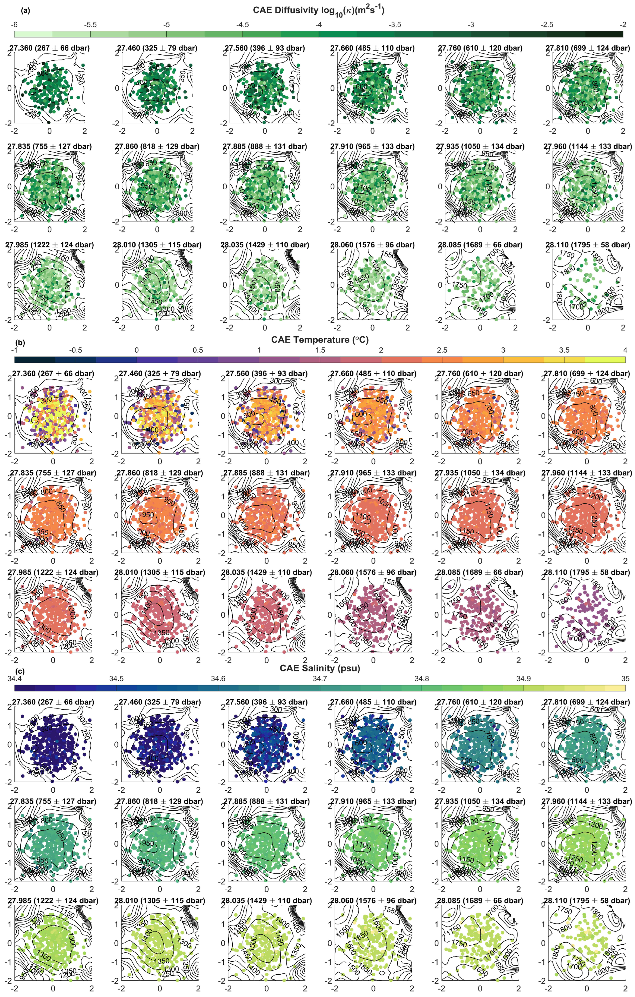
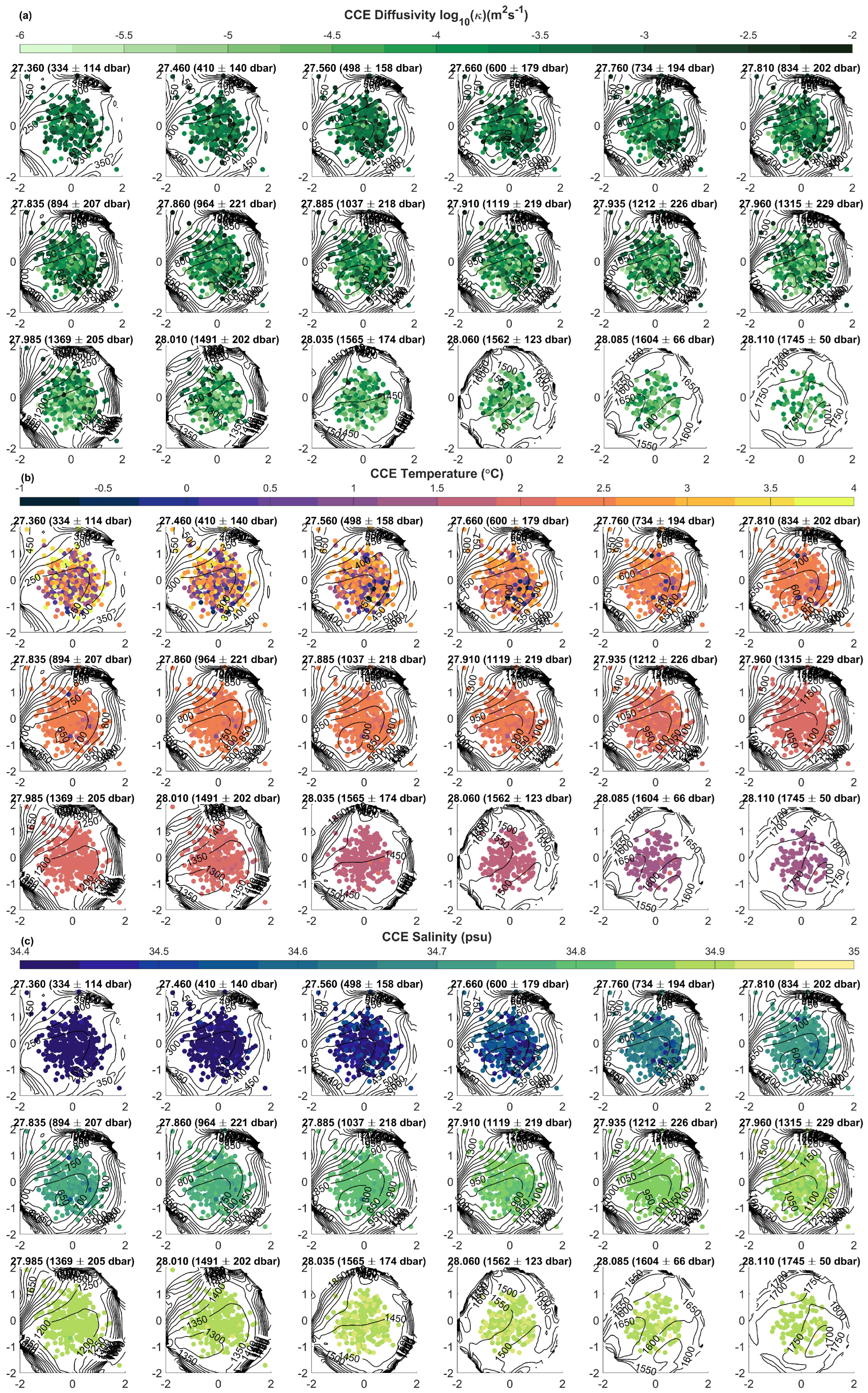
3.1. The Horizontal Structure of Composite Mesoscale Eddies and Their Impact on Mixing

By analyzing the trajectories of mesoscale eddies, which include 195 AEs and 203 CEs (Figure 4), we identified a total of 467 Argo profiles within AEs and 396 within CEs in the MR region. Both AEs and CEs cross the fronts. Most AEs move northward, and for CEs, the eddy movements appear to be relatively random, probably due to the limited number of eddies included in the analysis. The maximum number of Argo profiles captured by the same AE is 20, while that of CE is 13, and most AEs (CEs) capture less than 5 Argo profiles during the eddy lifespan. The average radius and lifetime of AEs are 65.79 km and 167.27 days, while those of CEs are 62.24 km and 121.45 days, respectively. In addition, we validated the effectiveness of our mesoscale eddy composite method by calculating the vertical variables averaged within 195 AEs and 203 CEs, as illustrated in Figure 5. The mean diapycnal mixing within CEs and AEs ranged from O ( 10 6 ) to O ( 10 2 )   m 2 s 1 for the full depth, with slightly higher mixing values for the CEs than for the AEs (Figure 5e,f), which is consistent with the results of [13] (their Figure 5e,f). That indicates CEs in this region contribute more intensive diapycnal mixing than AEs. Ref. [50] used high-resolution measurements of horizontal velocity from EM-APEX floats to investigate a mechanism of internal wave breaking inside mesoscale eddies in the standing meander near the Macquarie Ridge. They found stronger energy exchange from the background mean flow to internal waves within cyclonic eddies (CEs) compared to anticyclonic eddies (AEs). Therefore, the mesoscale eddy composite analysis, especially using the criterion of DHT less than 1.6 m, performed well in the MR region.
To investigate the horizontal structures of composite mesoscale eddies and their impact on mixing across various neutral surfaces, we depicted the horizontal distributions of diffusivity ( κ ), conservative temperature, and absolute salinity within 2 times the radius (2R) of a composite anticyclonic eddy (CAE) and cyclonic eddy (CCE) in Figure 6 and Figure 7, respectively. The κ and conservative temperature within both CAE and CCE decrease with depth of the neutral surface (Figure 5b,e, Figure 6a,b and Figure 7a,b), while absolute salinity increase (Figure 5c, Figure 6c and Figure 7c). Notably, the κ within CCE is one to two orders of magnitude higher than that within CAE on the same neutral surfaces. For instance, κ within CCE exceeds O ( 10 3 )   m 2 s 1 on 27.835 kgm 3 (Figure 7a), compared to κ within CAE is O ( 10 5 )   m 2 s 1 on the same neutral surface (Figure 6a).
The maximum κ for CAE typically occurs around 1 to 1.5 times the radius on neutral surfaces ranging from 27.36 to 28.11 kgm 3 (Figure 6a and Table 2). Notably, within 2R of CAE, κ values exceeding O ( 10 3 )   m 2 s 1 are observed above the above the 27.76 kgm 3 neutral surface, with conservative temperature below 1 °C and absolute salinity below 34.5 psu (Figure 6b,c). Moreover, the maximum κ for CCE depicts along its edge (1R) across neutral surfaces ranging from 27.36 to 28.11 kgm 3 (Figure 7a). In particular, the elevated κ around the periphery of CCE (1R, Figure 7a) corresponded to conservative temperature exceeding 3.5 °C and absolute salinity surpassing 34.5 psu above 27.66 kgm 3 (Figure 7b,c). Although the maximum mean value of κ for CCE shows at 1.5∼2R (Table 2), this may be due to the limited number of Argo profiles in this region. In contrast, within 1R of CCE, the mean values of κ are much larger than that of CAE (Table 2).
The closed isobars depict the horizontal configuration of CAE and CCE across various neutral surfaces in Figure 6 and Figure 7. Due to the smaller mean radius of CEs compared to AEs, the isobars within the normalized 2R of CCE are denser than those within CAE on equivalent neutral surfaces. This also resulted in the different location of the higher κ values in the horizontal distribution of CCE and CAE, with CCE exhibiting peak κ values at 0.5R∼1R and CAE at R∼1.5R. Additionally, the closed isobars outline the shape of CAE from 27.36 to 28.085 kgm 3 (1689 ± 66 dbar, the pressure is derived from the mean pressure values and their standard deviation (STD) on the neutral surface of 28.085 kgm 3 , hereinafter referred to as pressure ± STD/dbar) and from 27.36 to 28.01 kgm 3 (1491 ± 202 dbar) for CCE. The consistent vertical variation trends of variables for AEs from the sea surface to 28.085 kgm 3 (Figure 5) suggested a Taylor column shape for CAE from the sea surface to the neutral surface of 28.085 kgm 3 . Analogously, a similar shape of CAE for CCE from the sea surface to 28.01 kgm 3 is constructed.

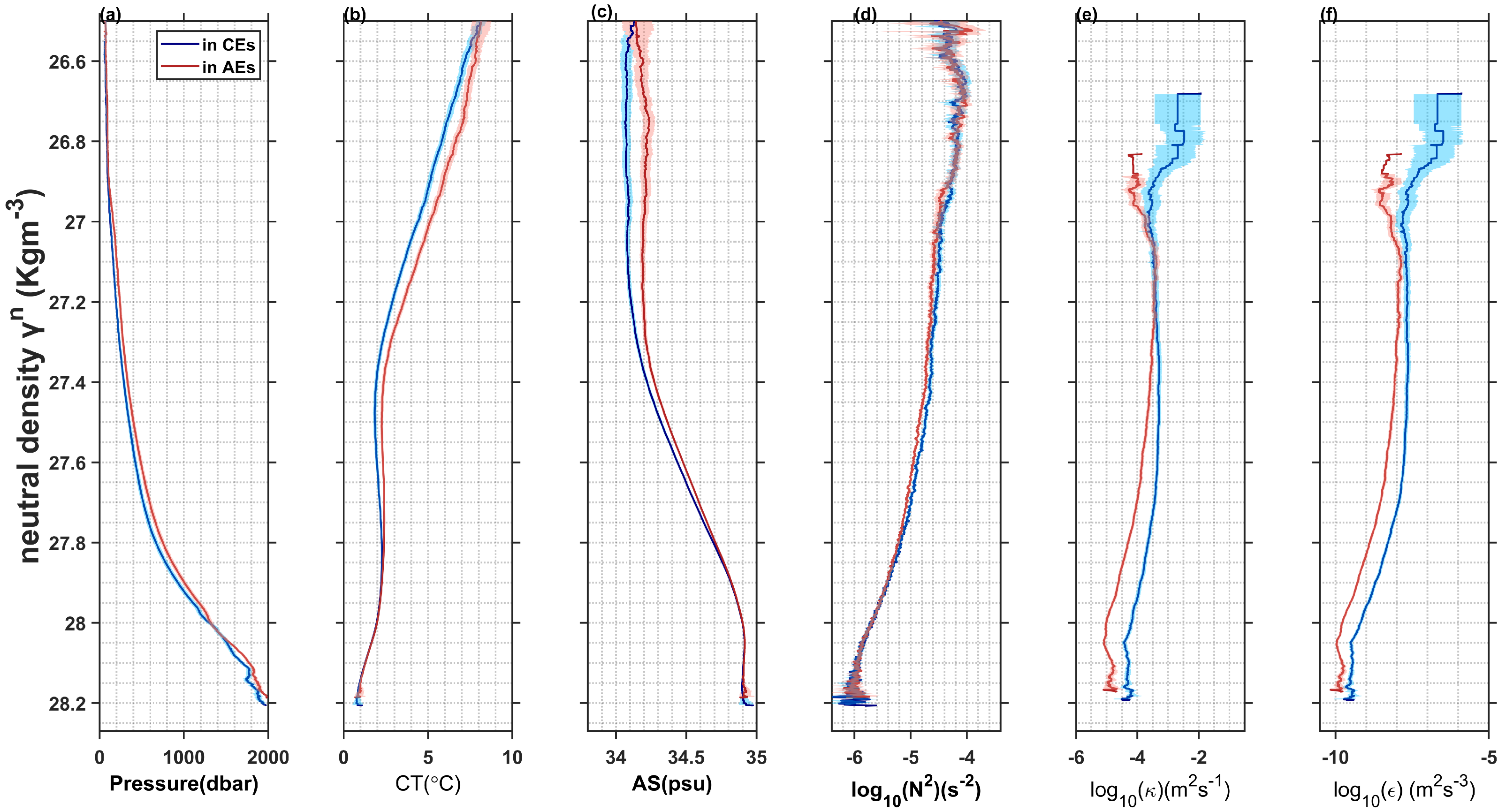
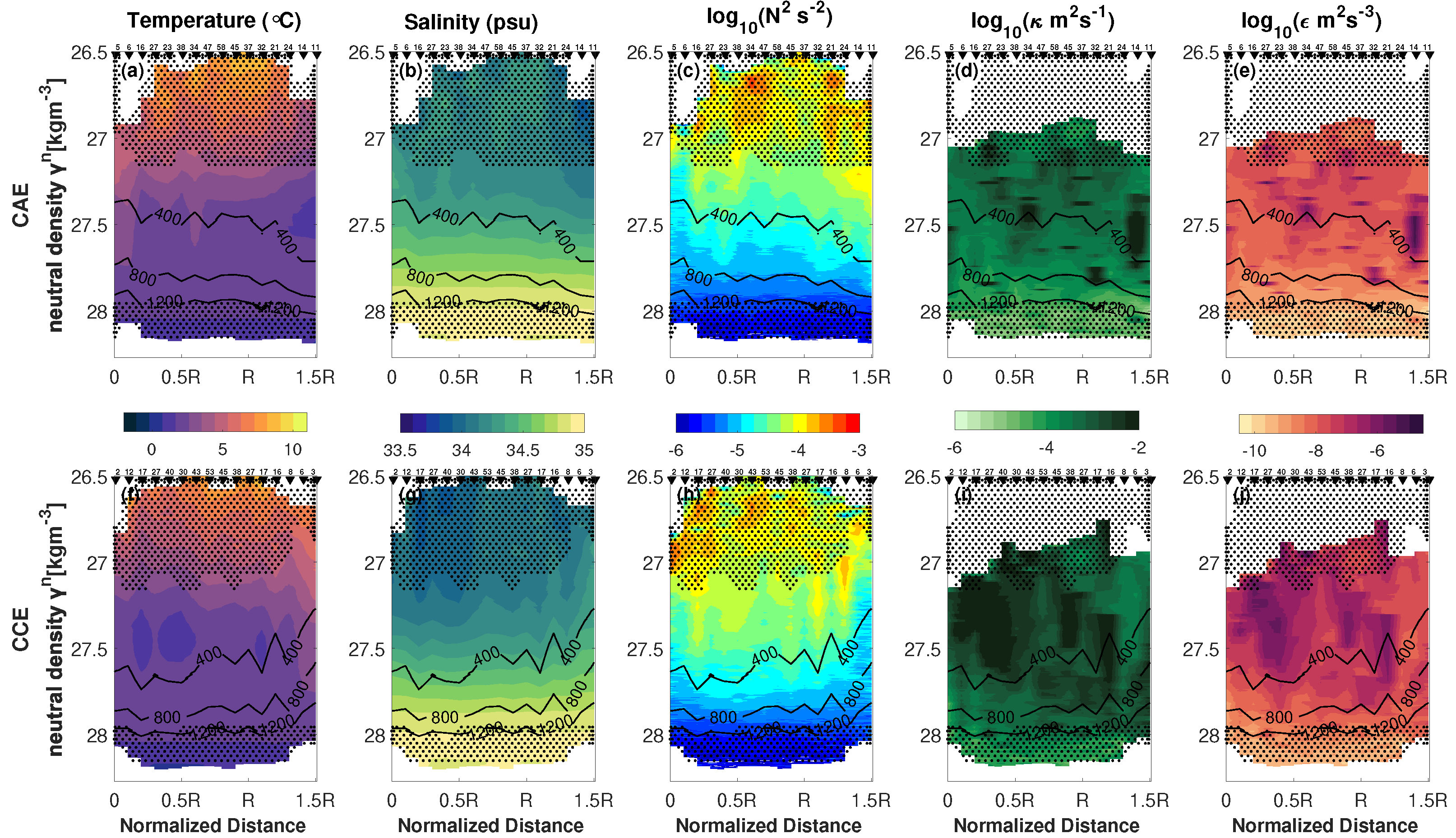
3.2. The Vertical Structure of Composite Mesoscale Eddies and Their Influence on Mixing

The distance of the Argo profile relative to the center of the eddy in which it is located was normalized by the eddy radius. The state parameters associated with mixing within the eddy were averaged over each neutral surface to obtain its radial-vertical spatial distribution characteristics (Figure 8). The radial coordinates were set from the eddy center to 1.5 times the eddy radius (1.5R) and divided into intervals of ∼0.1R, with the number of Argo profiles per interval placed at the top of the subplots. The trends of isobars within the eddies show that the isobars of CAE gradually deepen from the eddy center towards 1.5R (Figure 8a–e), in contrast to the trend of isobars of CCE (Figure 8f–j). Since the mean radius of AEs is larger than that of CEs in our study area, the isobars in CAE are sparser than those in CCE for the same pressure difference. The vertical distributions of conservative temperature along the eddy radius are shown in Figure 8a,f. Above the neutral surface of 27 kgm 3 , the temperatures of both CAE and CCE are high, and the conservative temperatures of CAE are significantly higher than those of CCE. Within the 0.6R range of CCE, a cold water mass of approximately 1 °C appears between the neutral surfaces of 27.4 and 27.6 kgm 3 . Vertical distributions of absolute salinity are shown in Figure 8b,g. The distribution of high salinity within the 1R range of CAE is localized and discontinuous, particularly at depths shallower than 400 dbar. In contrast, the distribution of low salinity is continuous within the 1R range of CCE, especially around 0.5R and at depths shallower than 400 dbar. Below 400 dbar, salinity in both CAE and CCE exhibit a gradient, with isohalines nearly parallel to the horizontal neutral surfaces, and absolute salinity increases with depth.
The buoyancy frequency ( N 2 ) as a characterization of the ocean stratification is shown in Figure 8c,h. There is no significant difference between the effects of CAE and CCE on ocean stratification. Both show a decrease in N 2 with depth, which is particularly pronounced in the upper 400 dbar, with a decrease of two orders of magnitude. It is noteworthy that both CAE and CCE show significant N 2 maxima at about 0.5R and 1R, reaching about 10 3 s 2 . Below 400 dbar, the stratification gradually decreases, and the N 2 isobars remain nearly horizontal along the neutral surfaces. In addition, minimum stratification values ( 10 5 s 2 ) are present in the center of CAE and the periphery of CCE (1.3R to 1.5R) under 27.3 kgm 3 . However, the limited number of Argo profiles at these specific locations may introduce high uncertainties.
Figure 8d,i shows the radial-vertical spatial distribution of mixing rates ( κ ) induced by CAE and CCE, respectively. The overall effect of CCE on κ is larger, typically by one to two orders of magnitude, compared to CAE. κ decreases with depth, and distinct peak κ values are found at 0.5R, R, and 1.5R for both CAE and CCE, with values of about O ( 10 3 )   m 2 s 1 for CAE and values up to O ( 10 2 )   m 2 s 1 for CCE. For instance, the maximum values of κ (over O ( 10 3 )   m 2 s 1 ) for CAE occur at ∼1.5R on the neutral surface of 27.5 kgm 3 . Conversely, for CCE the peak κ (over O ( 10 2 )   m 2 s 1 ) are found at 0∼0.5R and ∼1R above 400 dbar. In addition, Table 3 and Table 4 provide detailed distributions of mean κ values along the CAE and CCE center to 2R on neutral surfaces from 27.4 to 28 kgm 3 . The peak κ is located at the edge of CAE (0.5R∼1.5R) above 27.8 kgm 3 , then κ gradually decreases with depth, and the peak moves inwards to the center of CAE (0∼0.5R). By contrast, the CCE exhibits strong mixing at its center above 27.6 kgm 3 , then κ decreases outwards to the edge (1.5R–2R) with depth. Due to the limited number of Argo profiles located within 1.5R∼2R of CCE, the uncertainties associated with the mixing values increase in this region. Consequently, the enhanced κ associated with CCE appears to shift outwards from its center for neutral densities below 27.6 kgm 3 (Figure 8i and Table 4).
Figure 8e,j show the radial-vertical spatial distributions of dissipation rate ( ε ) within CAE and CCE. The distributions of ε are closely related to κ . The influence depth of AEs on ε (remaining at O ( 10 8 ) m 2 s 3 ) is about 800 dbar, while that of CEs is much deeper even up to 1200 dbar. Due to the limited number of contributing Argo profiles shallower than the neutral surface of 27 kgm 3 and deeper than the neutral surface of 28 kgm 3 , these two layers within CAE and CCE are almost covered by stipples.
The 3D structures of κ within CAE and CCE are shown in Figure 9. CCE affects κ at a deeper depth compared to CAE, with κ remaining at O ( 10 4 )   m 2 s 1 . CAE affects κ at a shallower depth, mainly around the neutral surface of 27.8 kgm 3 (680 ± 124 dbar), resulting in a northward shift of the high-mixing zone. In contrast, CCE exhibits enhanced κ at its bottom edge, while the high-mixing region of CAE departs from the 2R boundary at around 900 dbar. In summary, CAE and CCE exhibit similar patterns of mixing enhancement, i.e., as the depth increases, the intensified mixing of both shifts from the eddy center to the edge and then back to the center, only with different turning depths, as illustrated in Figure 9, Table 3 and Table 4.

4. Discussion and Conclusions

To quantify diapycnal mixing induced by composite mesoscale eddies in a standing meander of the ACC, a grand challenge is to reduce the effects of frontal shifts. This is because previous studies have found not only enhanced diapycnal mixing within frontal zones of the ACC [3,6,10,13], but also notable meridional fluctuations in fontal position over the years [33,51]. Therefore, in comparison to referencing climatological data indicating stable front positions (as provided by the World Ocean Atlas) for selecting Argo profiles for mesoscale eddy compositing in the ACC, the improved composite method performs well when employing the criterion of DHT less than 1.6 m in the present study.
Three supportive features prove the effective composite method. First, each DHT value is associated with a specific hydrographic profile in the ACC (e.g., [27,33]). According to the GEM climatological data [34,35], we employed 1.6 m DHT contour as the northern boundary of the ACC (the northern boundary of the ACC is generally considered to be the SAFN, Figure 1), which helps to select over 20 years Argo profiles carefully and reduces the influence of frontal zonal shifts on the multi-year for the composite (Figure 2). Therefore, we obtained the homogeneity and similarity of water mass properties in the Macquarie Ridge (MR) region (Figure 3).
Second, the emergence of the “Taylor column” represents a potential consequence of fluid flow interacting with an isolated topographic feature [52]. Ref. [53] dimensionally analyzed anticyclonic eddies with Taylor columns shape exist in the ACC. Ref. [54] reported the first anticyclonic circulation with Taylor column character based on field observation. And its vertical influence spans from the sea surface to the seafloor. Ref. [39] revealed the eddies signature can reach deep to ∼3000 m in the MR region through two years mooring. Moreover, a high-resolution global ocean simulation presented that mesoscale eddies in the ACC are the deepest in the world [55]. A composite structure of ACC mesoscale eddies indicated their penetration to depths of at least 2000 m based on Argo floats and satellite altimeter data [4]. Finally, a recent study first characterized a cyclonic eddy structure in the MR region; the perturbations of isopycnals extend to 1500 m [12]. Therefore, the 3D structures of mesoscale eddies in the ACC are known to exhibit a Taylor column shape, with their vertical influence spanning from the sea surface to the seafloor or at least to depths of 1000–2000 m. In the present study, the composite anticyclonic eddy (CAE) extends in depth from the sea surface to the 28.085 kgm 3 neutral surface (1689 ± 66 dbar) with a Taylor column shape, while the composite cyclonic eddy (CCE) reaches from the sea surface to the 28.01 kgm 3 neutral surface (1491 ± 202 dbar) (Figure 6 and Figure 7).
Third, the variation range and trend of the mean vertical diffusivity and dissipation rate in AEs/CEs are consistent with previous findings in the standing meander near the MR [13], and CEs enhance mixing slightly higher than AEs (Figure 5e,f). It is well known that standing meanders are associated with high EKE and topographic features in the ACC [22]. However, ref. [13] found there is no correlation between enhanced mixing above 1600 dbar and local rough topography in the MR region. In general, the distribution of turbulent mixing is determined by the breaking of internal waves in the interior of the Southern Ocean [5,11]. Additionally, this is one of the assumptions of the fine-scale parameterization method used to estimate diapycnal mixing in this study. Recently, ref. [50] characterized the internal wave field and investigated their interactions with mesoscale eddies and the ACC mean flow using continuous high-frequency observation data from EM-APEX floats. They found that the strongest energy transfer is from the background mean flow to the internal waves in CEs, while there is no energy transfer from the mean flow to the internal waves in AEs in the MR region. That indicates stronger turbulent mixing occurs in CEs through the breaking of internal waves compared to AEs. In the present study, the peak values of the diapycnal diffusivity ( κ ) within the composite cyclonic eddy (CCE) were one to two orders of magnitude higher than those within the composite anticyclonic eddy (CAE) on the same neutral surfaces. Vertically, the CCE affected κ down to approximately 1200 dbar, with κ exceeding O ( 10 4 ) m 2 s 1 . In contrast, the CAE influenced κ only down to about 800 dbar, with κ exceeding O ( 10 4 ) m 2 s 1 (Figure 6, Figure 7 and Figure 8). Furthermore, observations have highlighted the role of submesoscale instabilities that occur along the edges of mesoscale eddies [56,57], ref. [6] specifically found enhanced mixing at the edge of a cyclonic eddy in the ACC. The observed enhanced mixing at mesoscale eddy edges in this study (Figure 9, Table 2, Table 3 and Table 4). That suggests the potential occurrence of submesoscale instabilities below the mixing layer. Future work will further investigate the mechanisms of turbulent mixing in mesoscale eddies using high-resolution observations and numerical simulations.
In summary, to reconstruct the 3D structure of mesoscale eddies in the ACC hotspot region and to investigate their impact on diapycnal mixing, we utilize a 27-year multi-satellite eddy dataset and Argo profiles with 2-m vertical resolution. Using the improved composite method, Argo profiles are carefully selected for the composite, which reduces the influence of frontal zonal shifts on the multi-year composite eddy data. The improved mesoscale eddy composite method also enhances the homogeneity and similarity of water mass properties in the MR region, leading to an increase in the accuracy of mesoscale eddy structures. In addition, the effect of eddy shapes on mixing is eliminated, and the observed shear-strain ratio R ω = 6 is used, resulting in results consistent with the magnitude of eddy-induced mixing observed in previous studies [13].
The following conclusions are drawn: Both CAE and CCE exhibit a Taylor column shape, with CAE extending in depth from the sea surface to 28.085 kgm 3 (1689 ± 66 dbar) and CCE extending from the sea surface to 28.01 kgm 3 (1491 ± 202 dbar). Horizontally, CCE enhances κ by one to two orders of magnitude compared to CAE on the same neutral surfaces, and maximum κ values occur at 0.5R, 1R, and 1.5R on the same neutral surfaces for both CAE and CCE. Vertically, CCE affects κ down to approximately 1200 dbar, with κ exceeding O ( 10 4 ) m 2 s 1 . In contrast, CAE influences κ only down to about 800 dbar, with κ exceeding O ( 10 4 ) m 2 s 1 . And below the maximum depth of mesoscale eddy influence, κ values decrease with increasing neutral density. Therefore, these new insights will help to better understand the influence of mesoscale eddies on diapycnal mixing in the Southern Ocean, and thus improve the prediction of the large-scale currents and global climate change.

Author Contributions

Conceptualization, Y.B., C.M. and H.E.P.; Formal analysis, Y.B. and A.C.; Methodology, Y.B., C.M. and H.E.P.; Supervision, C.M., Y.L. and H.E.P.; Validation, Y.B. and A.C.; Writing—original draft, Y.B.; Writing—review and editing, C.M., Y.L., H.E.P. and A.C.; Funding acquisition, C.M. All authors have read and agreed to the published version of the manuscript.

Funding

This research was supported by the National Basic Research Priorities Program of China under grants 2015CB954300. Y. Bao received support from the Foundation of China Scholarship Council (201906330005). Y. Luo was supported by the National Natural Science Foundation of China (42230405 and 41976006).

Data Availability Statement

Data are available in Section 2.

Acknowledgments

The authors thank AVISO+ and their team for providing the new global Mesoscale Eddy Trajectory Atlas. Also, we thank IFREMER for offering Argo data, which was collected and made freely available by the International Argo Program and the national programs.

Conflicts of Interest

The authors declare no conflicts of interest.

References

  1. Whalen, C.B.; MacKinnon, J.A.; Talley, L.D. Large-scale impacts of the mesoscale environment on mixing from wind-driven internal waves. Nat. Geosci. 2018, 11, 842–847. [Google Scholar] [CrossRef]
  2. Marshall, J.; Speer, K. Closure of the meridional overturning circulation through Southern Ocean upwelling. Nat. Geosci. 2012, 5, 171–180. [Google Scholar] [CrossRef]
  3. Rintoul, S.R. The global influence of localized dynamics in the Southern Ocean. Nature 2018, 558, 209–218. [Google Scholar] [CrossRef]
  4. Frenger, I.; Münnich, M.; Gruber, N.; Knutti, R. Southern Ocean eddy phenomenology. J. Geophys. Res. Ocean. 2015, 120, 7413–7449. [Google Scholar] [CrossRef]
  5. Waterman, S.; Naveira Garabato, A.C.; Polzin, K.L. Internal Waves and Turbulence in the Antarctic Circumpolar Current. J. Phys. Oceanogr. 2013, 43, 259–282. [Google Scholar] [CrossRef]
  6. Meyer, A.; Sloyan, B.M.; Polzin, K.L.; Phillips, H.E.; Bindoff, N.L. Mixing Variability in the Southern Ocean. J. Phys. Oceanogr. 2015, 45, 966–987. [Google Scholar] [CrossRef]
  7. Sheen, K.L.; Garabato, A.C.; Brearley, J.A.; Meredith, M.P.; Polzin, K.L.; Smeed, D.A.; Forryan, A.; King, B.A.; Sallée, J.B.; St. Laurent, L.; et al. Eddy-induced variability in Southern Ocean abyssal mixing on climatic timescales. Nat. Geosci. 2014, 7, 577–582. [Google Scholar] [CrossRef]
  8. Arzel, O.; de Verdière, A.C. Can we infer diapycnal mixing rates from the world ocean temperature-salinity distribution? J. Phys. Oceanogr. 2016, 46, 3751–3775. [Google Scholar] [CrossRef]
  9. Dove, L.A.; Thompson, A.F.; Balwada, D.; Gray, A.R. Observational Evidence of Ventilation Hotspots in the Southern Ocean. J. Geophys. Res. Ocean. 2021, 126, e2021JC017178. [Google Scholar] [CrossRef]
  10. St. Laurent, L.; Naveira Garabato, A.C.; Ledwell, J.R.; Thurnherr, A.M.; Toole, J.M.; Watson, A.J. Turbulence and diapycnal mixing in drake passage. J. Phys. Oceanogr. 2012, 42, 2143–2152. [Google Scholar] [CrossRef]
  11. Sheen, K.L.; Brearley, J.A.; Naveira Garabato, A.C.; Smeed, D.A.; Waterman, S.; Ledwell, J.R.; Meredith, M.P.; St. Laurent, L.; Thurnherr, A.M.; Toole, J.M.; et al. Rates and mechanisms of turbulent dissipation and mixing in the Southern Ocean: Results from the Diapycnal and Isopycnal Mixing Experiment in the Southern Ocean (DIMES). J. Geophys. Res. Ocean. 2013, 118, 2774–2792. [Google Scholar] [CrossRef]
  12. Patel, R.S.; Phillips, H.E.; Strutton, P.G.; Lenton, A.; Llort, J. Meridional Heat and Salt Transport Across the Subantarctic Front by Cold-Core Eddies. J. Geophys. Res. Ocean. 2019, 124, 981–1004. [Google Scholar] [CrossRef]
  13. Cyriac, A.; Phillips, H.E.; Bindoff, N.L.; Polzin, K. Turbulent Mixing Variability in an Energetic Standing Meander of the Southern Ocean. J. Phys. Oceanogr. 2022, 52, 1593–1611. [Google Scholar] [CrossRef]
  14. Keppler, L.; Cravatte, S.; Chaigneau, A.; Pegliasco, C.; Gourdeau, L.; Singh, A. Observed Characteristics and Vertical Structure of Mesoscale Eddies in the Southwest Tropical Pacific. J. Geophys. Res. Ocean. 2018, 123, 2731–2756. [Google Scholar] [CrossRef]
  15. Zhan, P.; Krokos, G.; Guo, D.; Hoteit, I. Three-Dimensional Signature of the Red Sea Eddies and Eddy-Induced Transport. Geophys. Res. Lett. 2019, 46, 2167–2177. [Google Scholar] [CrossRef]
  16. Chaigneau, A.; Le Texier, M.; Eldin, G.; Grados, C.; Pizarro, O. Vertical structure of mesoscale eddies in the eastern South Pacific Ocean: A composite analysis from altimetry and Argo profiling floats. J. Geophys. Res. Ocean. 2011, 116. [Google Scholar] [CrossRef]
  17. Zhang, Z.; Wang, W.; Qiu, B. Oceanic mass transport by mesoscale eddies. Science 2014, 345, 322–324. [Google Scholar] [CrossRef] [PubMed]
  18. Sun, B.; Liu, C.; Wang, F. Global meridional eddy heat transport inferred from Argo and altimetry observations. Sci. Rep. 2019, 9, 1345. [Google Scholar] [CrossRef] [PubMed]
  19. Wang, H.; Qiu, B.; Liu, H.; Zhang, Z. Doubling of surface oceanic meridional heat transport by non-symmetry of mesoscale eddies. Nat. Commun. 2023, 14, 5460. [Google Scholar] [CrossRef]
  20. Sun, C.; Watts, D.R. Heat flux carried by the Antarctic Circumpolar Current mean flow. J. Geophys. Res. Ocean. 2002, 107, 2-1–2-13. [Google Scholar] [CrossRef]
  21. Talley, L.D. Closure of the global overturning circulation through the Indian, Pacific, and southern oceans. Oceanography 2013, 26, 80–97. [Google Scholar] [CrossRef]
  22. Chelton, D.B.; Schlax, M.G.; Samelson, R.M.; de Szoeke, R.A. Global observations of large oceanic eddies. Geophys. Res. Lett. 2007, 34. [Google Scholar] [CrossRef]
  23. Jia, F.; Wu, L.; Qiu, B. Seasonal Modulation of Eddy Kinetic Energy and Its Formation Mechanism in the Southeast Indian Ocean. J. Phys. Oceanogr. 2011, 41, 657–665. [Google Scholar] [CrossRef]
  24. Tamsitt, V.; Drake, H.F.; Morrison, A.K.; Talley, L.D.; Dufour, C.O.; Gray, A.R.; Griffies, S.M.; Mazloff, M.R.; Sarmiento, J.L.; Wang, J.; et al. Spiraling pathways of global deep waters to the surface of the Southern Ocean. Nat. Commun. 2017, 8, 172. [Google Scholar] [CrossRef] [PubMed]
  25. Foppert, A.; Donohue, K.A.; Watts, D.R.; Tracey, K.L. Eddy heat flux across the Antarctic Circumpolar Current estimated from sea surface height standard deviation. J. Geophys. Res. Ocean. 2017, 122, 6947–6964. [Google Scholar] [CrossRef]
  26. Patel, R.S.; Llort, J.; Strutton, P.G.; Phillips, H.E.; Moreau, S.; Conde Pardo, P.; Lenton, A. The Biogeochemical Structure of Southern Ocean Mesoscale Eddies. J. Geophys. Res. Ocean. 2020, 125, e2020JC016115. [Google Scholar] [CrossRef]
  27. Meijer, J.J.; Phillips, H.E.; Bindoff, N.L.; Rintoul, S.R.; Foppert, A. Dynamics of a Standing Meander of the Subantarctic Front Diagnosed from Satellite Altimetry and Along-Stream Anomalies of Temperature and Salinity. J. Phys. Oceanogr. 2022, 52, 1073–1089. [Google Scholar] [CrossRef]
  28. Cyriac, A.; Phillips, H.E.; Bindoff, N.L.; Mao, H.; Feng, M. Observational estimates of turbulent mixing in the southeast indian ocean. J. Phys. Oceanogr. 2021, 51, 2103–2128. [Google Scholar] [CrossRef]
  29. Gordon, A.L. An Antarctic oceanographic section along 170°E. Deep-Sea Res. Oceanogr. Abstr. 1975, 22, 357–377. [Google Scholar] [CrossRef]
  30. Rintoul, S.R.; Sokolov, S.; Williams, M.J.M.; Peña Molino, B.; Rosenberg, M.; Bindoff, N.L. Antarctic Circumpolar Current transport and barotropic transition at Macquarie Ridge. Geophys. Res. Lett. 2014, 41, 7254–7261. [Google Scholar] [CrossRef]
  31. Pegliasco, C.; Delepoulle, A.; Mason, E.; Morrow, R.; Faugère, Y.; Dibarboure, G. META3.1exp: A new global mesoscale eddy trajectory atlas derived from altimetry. Earth Syst. Sci. Data 2022, 14, 1087–1107. [Google Scholar] [CrossRef]
  32. Zhang, Z.; Zhang, Y.; Wang, W.; Huang, R.X. Universal structure of mesoscale eddies in the ocean. Geophys. Res. Lett. 2013, 40, 3677–3681. [Google Scholar] [CrossRef]
  33. Sokolov, S.; Rintoul, S.R. Circumpolar structure and distribution of the antarctic circumpolar current fronts: 2. Variability and relationship to sea surface height. J. Geophys. Res. Ocean. 2009, 114, C11019. [Google Scholar] [CrossRef]
  34. Meijers, A.J.; Bindoff, N.L.; Rintoul, S.R. Frontal movements and property fluxes: Contributions to heat and freshwater trends in the Southern Ocean. J. Geophys. Res. Ocean. 2011, 116, 1–17. [Google Scholar] [CrossRef]
  35. Meijers, A.J.; Bindoff, N.L.; Rintoul, S.R. Estimating the four-dimensional structure of the southern ocean using satellite altimetry. J. Atmos. Ocean. Technol. 2011, 28, 548–568. [Google Scholar] [CrossRef]
  36. Orsi, A.H.; Whitworth, T.; Nowlin, W.D. On the meridional extent and fronts of the Antarctic Circumpolar Current. Deep Sea Res. Part I Oceanogr. Res. Pap. 1995, 42, 641–673. [Google Scholar] [CrossRef]
  37. Sokolov, S.; Rintoul, S.R. Multiple Jets of the Antarctic Circumpolar Current South of Australia. J. Phys. Oceanogr. 2007, 37, 1394–1412. [Google Scholar] [CrossRef]
  38. Rintoul, S.R.; Bullister, J.L. A late winter hydrographic section from Tasmania to Antarctica. Deep Sea Res. Part I Oceanogr. Res. Pap. 1999, 46, 1417–1454. [Google Scholar] [CrossRef]
  39. Phillips, H.E.; Rintoul, S.R. Eddy variability and energetics from direct current measurements in the Antarctic Circumpolar Current south of Australia. J. Phys. Oceanogr. 2000, 30, 3050–3076. [Google Scholar] [CrossRef]
  40. Cressman, G.P. An Operational Objective Analysis System. Mon. Weather Rev. 1959, 87, 367–374. [Google Scholar] [CrossRef]
  41. Kunze, E.; Firing, E.; Hummon, J.M.; Chereskin, T.K.; Thurnherr, A.M. Global abyssal mixing inferred from lowered ADCP shear and CTD strain profiles. J. Phys. Oceanogr. 2006, 36, 1553–1576. [Google Scholar] [CrossRef]
  42. Henyey, F.S.; Wright, J.; Flatté, S.M. Energy and action flow through the internal wave field: An eikonal approach. J. Geophys. Res. 1986, 91, 8487. [Google Scholar] [CrossRef]
  43. Polzin, K.L.; Toole, J.M.; Schmitt, R.W. Finescale Parameterizations of Turbulent Dissipation. J. Phys. Oceanogr. 1995, 25, 306–328. [Google Scholar] [CrossRef]
  44. Cairns, J.L.; Williams, G.O. Internal wave observations from a midwater float, 2. J. Geophys. Res. 1976, 81, 1943–1950. [Google Scholar] [CrossRef]
  45. Bray, N.A.; Fofonoff, N.P. Available Potential Energy for MODE Eddies. J. Phys. Oceanogr. 1981, 11, 30–47. [Google Scholar] [CrossRef]
  46. Gregg, M.C.; D’Asaro, E.A.; Riley, J.J.; Kunze, E. Mixing efficiency in the ocean. Annu. Rev. Mar. Sci. 2018, 10, 443–473. [Google Scholar] [CrossRef]
  47. Osborn, T.R. Estimates of the Local Rate of Vertical Diffusion from Dissipation Measurements. J. Phys. Oceanogr. 1980, 10, 83–89. [Google Scholar] [CrossRef]
  48. de Boyer Montégut, C.; Madec, G.; Fischer, A.S.; Lazar, A.; Iudicone, D. Mixed layer depth over the global ocean: An examination of profile data and a profile-based climatology. J. Geophys. Res. Ocean. 2004, 109, 1–20. [Google Scholar] [CrossRef]
  49. Meyer, A.; Phillips, H.E.; Sloyan, B.M.; Polzin, K.L. Mixing (MX) Oceanographic Toolbox for EM-APEX * Float Data Applying Shear-Strain Finescale Parameterization; University of Tasmania: Tasmania, Australia, 2014. [Google Scholar]
  50. Cyriac, A.; Meyer, A.; Phillips, H.E.; Bindoff, N.L. Observations of internal wave interactions in a Southern Ocean standing meander. J. Phys. Oceanogr. 2023, 53, 1997–2011. [Google Scholar] [CrossRef]
  51. Kim, Y.S.; Orsi, A.H. On the variability of antarctic circumpolar current fronts inferred from 1992-2011 altimetry. J. Phys. Oceanogr. 2014, 44, 3054–3071. [Google Scholar] [CrossRef]
  52. Meredith, M.P.; Meijers, A.S.; Naveira Garabato, A.C.; Brown, P.J.; Venables, H.J.; Abrahamsen, E.P.; Jullion, L.; Messias, M. Circulation, retention, and mixing of waters within the Weddell-Scotia Confluence, Southern Ocean: The role of stratified Taylor columns. J. Geophys. Res. Ocean. 2015, 120, 547–562. [Google Scholar] [CrossRef]
  53. Perissinotto, R.; Duncombe Rae, C.M. Occurrence of anticyclonic eddies on the Prince Edward Plateau (Southern Ocean): Effects on phytoplankton biomass and production. Deep Sea Res. Part A Oceanogr. Res. Pap. 1990, 37, 777–793. [Google Scholar] [CrossRef]
  54. Meredith, M.P.; Watkins, J.L.; Murphy, E.J.; Cunningham, N.J.; Wood, A.G.; Korb, R.; Whitehouse, M.J.; Thorpe, S.E.; Vivier, F. An anticyclonic circulation above the Northwest Georgia Rise, Southern Ocean. Geophys. Res. Lett. 2003, 30, 1–5. [Google Scholar] [CrossRef]
  55. Petersen, M.R.; Williams, S.J.; Maltrud, M.E.; Hecht, M.W.; Hamann, B. A three-dimensional eddy census of a high-resolution global ocean simulation. J. Geophys. Res. Ocean. 2013, 118, 1759–1774. [Google Scholar] [CrossRef]
  56. Adams, K.A.; Hosegood, P.; Taylor, J.R.; Sallée, J.B.; Bachman, S.; Torres, R.; Stamper, M. Frontal circulation and submesoscale variability during the formation of a southern ocean mesoscale eddy. J. Phys. Oceanogr. 2017, 47, 1737–1753. [Google Scholar] [CrossRef]
  57. Yang, Q.; Nikurashin, M.; Sasaki, H.; Sun, H.; Tian, J. Dissipation of mesoscale eddies and its contribution to mixing in the northern South China Sea. Sci. Rep. 2019, 9, 556. [Google Scholar] [CrossRef] [PubMed]
Figure 1. (a) locations of all Argo profiles within the effective shape contours of AEs, separated by different dynamic heights (DHT/m) at 100 dbar relative to 2000 dbar in the study area. The colors of the spots represent the DHT range as follows: purple (<0.83 m), cyan (0.83∼1.1 m), green (1.1∼1.6 m), and yellow (1.6∼1.98 m). The color-filled contour represents the bathymetry, deriving from ETOPO1 data. The colored curves represent the front position, derived from the average of weekly climate front data from 2009 to 2013, with yellow for SAFN, cyan for SAF, and orange for PF. (b) same as (a), but for the profiles inside of CEs. (c) histogram of the number of Argo profiles within AEs and CEs with DHT less than 1.6 m, showing the values in each latitude interval between 48°S and 61°S.
Remotesensing 16 01863 g001
Figure 2. Hydrographic properties from all Argo profiles inside of mesoscale eddy shapes in the study area. (a) conservative temperature, (b) absolute salinity on neutral density surfaces vary with DHT (100/2000 dbar). A total of 751 (405) Argo profiles were selected inside AEs (CEs). The vertical red dotted-dashed lines indicate the boundaries of the five DHT intervals, with their corresponding values labeled on the top panel.
Remotesensing 16 01863 g002
Figure 3. Hydrographic properties inside of AEs and CEs within the four DHT intervals. T-S and their mean values are represented by solid and dashed lines of different colors. Neutral density is shown in black contours. The number of Argo profiles within each interval is shown in parentheses, following the ranges of DHT for each panel.
Remotesensing 16 01863 g003
Figure 4. Trajectories of eddies containing Argo profiles in the Macquarie Ridge region. (a) The yellow pentagrams indicate the center positions of 195 AEs when they initially captured Argo profiles. The red asterisks indicate the location of eddy centers during their movement, and the red polylines indicate the trajectories. (b) Same as (a), but the yellow pentagrams, blue asterisks, and polylines are for 203 CEs. The color-filled contour represents the bathymetry, deriving from ETOPO1 data. The colored curves represent the fronts’ positions, deriving from the average of weekly climate front data from 2009 to 2013, with yellow for the Northern Sub-Antarctic Front (SAFN), cyan for the Sub-Antarctic Front (SAF), and orange for the Polar Front (PF).
Remotesensing 16 01863 g004
Figure 5. The mean vertical values derived from 467 Argo profiles within AEs and 396 within CEs on neutral surfaces from 26.5 to 28.27 kgm 3 . (a) Pressure, (b) conservative temperature, (c) absolute salinity, (d) buoyancy frequency, (e) diffusivity, and (f) dissipation rate. The shading is the error bar, which shows 90% confidence intervals using the bootstrap method.
Remotesensing 16 01863 g005
Figure 6. (a) The distribution of diffusivity on neutral surfaces from 27.36 to 28.11 kgm 3 (the pressure is derived from the mean pressure values and its standard deviation on each neutral surface) about CAE, (b) same as (a), but for conservative temperature, (c) same as (a), but for absolute salinity. The contour lines are drawn every 50 dbar. The dots directly denote diffusivity/conservative temperature/absolute salinity from the Argo profiles.
Remotesensing 16 01863 g006
Figure 7. Same as Figure 6, but for CCE.
Remotesensing 16 01863 g007
Figure 8. Vertical structures of conservative temperature (a), absolute salinity (b), buoyancy frequency (c), diffusivity (d), and dissipation rate (e) within CAE along the eddy center to 1.5 times the normalized radius (1.5R) from 26.5 to 28.27 kgm 3 neutral surface. (fj) are the same as (ae), but within CCE. The number of Argo profiles is labeled at the top of all panels, solid black lines represent isobars with intervals of 400 dbar, and the stipples indicate grid points with less than 75% data.
Remotesensing 16 01863 g008
Figure 9. 3D structure of diffusivity ( log 10 ( κ ) in m 2 s 1 ) within 2R of composite mesoscale eddies in neutral density coordinate for CAE (a) and CCE (b), with Δ x = Δ y = 2R. The pressure coordinates are derived from the mean pressure values and their standard deviation (STD/dbar) on each neutral surface.
Remotesensing 16 01863 g009
Table 1. The procedures of selecting Argo profiles.
AEsCEs
Step 1Number of Argo profiles inside corresponding eddies782740
Number of Argo profiles with consistent SLA sign (AVISO) and eddy polarity777 (positive)579 (negative)
Number of Argo profiles with consistent SLA sign (Argo) and eddy polarity753 (positive)423 (negative)
Number of Argo profiles with consistent SLA sign (AVISO & Argo) and eddy polarity751 (positive)405 (negative)
Step 2Different DHT range (m)<0.830.83∼1.11.1∼1.61.6∼1.98<0.830.83∼1.11.1∼1.61.6∼1.98
Number of Argo profiles classified by DHT882041752821211481279
Step 3Number of Composite eddy profiles (DHT < 1.6)467396
Number of Composite eddy profiles (Normalized R < 2)448388
Number of Composite eddy profiles (Normalized R < 1.5)438384
Table 2. Mean values of κ (× ( 10 4 )   m 2 s 1 ) and their 90% confidence intervals within CAE and CCE, along eddy center to 2 times the normalized radius (2R) from 27.36 to 28.11 kgm 3 neutral surface.
CAE
Number of Argo Profiles
κ CCE
Number of Argo Profiles
κ
0∼0.5R776.62 ± 1.3510246.00 ± 2.25
0.5R∼1R2227.92 ± 0.6821420.00 ± 0.84
R∼1.5R12836.00 ± 2.646728.00 ± 1.05
1.5R∼2R216.91 ± 1.54573.00 ± 9.24
Table 3. Mean values of κ ( 10 4 )   m 2 s 1 ) and their 90% confidence intervals within CAE, along eddy center to 2 times the normalized radius (2R) on neutral surfaces from 27.4 to 28 kgm 3 . The maximum mean value of κ on each neutral surface is highlighted in boldface.
Neutral Surface/ kgm 3
(Pressure ± STD/dbar)
0∼0.5R0.5R∼RR∼1.5R1.5R∼2R
27.4
(287 ± 71 dbar)
4.84 ± 2.1849 ± 724.56 ± 1.854.55 ± 1.67
27.5
(353 ± 84 dbar)
2.32 ± 0.559.27 ± 7.5195 ± 1505.74 ± 2.71
27.6
(430 ± 100 dbar)
2.64 ± 1.375.84 ± 2.91109 ± 1775.97 ± 4.44
27.7
(530 ± 117 dbar)
2.93 ± 1.232.88 ± 1.063.05 ± 1.542.02 ± 1.05
27.8
(680 ± 124 dbar)
1.46 ± 0.601.56 ± 0.6532 ± 501.27 ± 1.03
27.9
(934 ± 134 dbar)
0.99 ± 0.400.90 ± 0.270.69 ± 0.170.58 ± 0.35
28
(1273 ± 118 dbar)
0.56 ± 0.270.25 ± 0.070.24 ± 0.090.11 ± 0.10
Table 4. Mean values of κ ( 10 3 )   m 2 s 1 ) and their 90% confidence intervals within CCE, along eddy center to 2 times the normalized radius (2R) on neutral surfaces from 27.4 to 28 kgm 3 . The maximum mean value of κ on each neutral surface is highlighted in boldface.
Neutral Surface/ kgm 3
(Pressure ± STD/dbar)
0∼0.5R0.5R∼RR∼1.5R1.5R∼2R
27.4
(287 ± 71 dbar)
24.70 ± 21.66.50 ± 7.94.50 ± 5.202.60 ± 3.20
27.5
(353 ± 84 dbar)
13.60 ± 12.902.20 ± 0.964.40 ± 5.001.90 ± 2.80
27.6
(430 ± 100 dbar)
5.70 ± 4.601.60 ± 0.563.80 ± 3.901.00 ± 1.50
27.7
(530 ± 117 dbar)
1.10 ± 0.592.70 ± 1.103.80 ± 2.6013.8 ± 28.4
27.8
(680 ± 124 dbar)
0.71 ± 0.400.95 ± 0.362.30 ± 1.502.40 ± 3.50
27.9
(934 ± 134 dbar)
0.39 ± 0.270.54 ± 0.140.92 ± 0.3211.3 ± 23.0
28
(1273 ± 118 dbar)
0.74 ± 0.940.32 ± 0.120.70 ± 0.560.88 ± 3.6
Disclaimer/Publisher’s Note: The statements, opinions and data contained in all publications are solely those of the individual author(s) and contributor(s) and not of MDPI and/or the editor(s). MDPI and/or the editor(s) disclaim responsibility for any injury to people or property resulting from any ideas, methods, instructions or products referred to in the content.

