Long-Term Sea Level Periodicities over the European Seas from Altimetry and Tide Gauge Data

Abstract

This study investigates the long-term temporal patterns of sea level changes by analyzing monthly tide gauge data from 1950 to 2022 (42 to 72 years) along the European coastline and monthly altimetry data from 1992 to 2024 in the surrounding European seas. The primary focus is on signals with periods longer than 5 years. The application of wavelet-based approaches and multiresolution analysis has enabled the isolation of signals with periods of approximately 8 and 16 years. However, the latter has only been observed in tide gauge data, as the altimetry time series is not sufficiently long. The same analysis was applied to the North Atlantic Oscillation (NAO) and Atlantic Multidecadal Oscillation (AMO) indices, which enabled the detection of the same signals. The reported multiyear signals of sea level are correlated with NAO and AMO indices, particularly during the period spanning from 1975 to 2010.

1. Introduction

The rate of increase in global sea level (SL) has accelerated since the late 19th century. From 1900 to 2009, measurements obtained from tide gauges (TG) indicated a mean rate of SL rise of 1.7 mm/year [1]. Over the last three decades, altimetry measurements have indicated a global SL rise of approximately 3.3 mm/year [2], with slightly higher values observed in Europe [3]. The rate of increase is exhibiting an exponential growth pattern [4]. This increase in SL is a consequence of global warming, which occurs in two distinct ways. The first mechanism by which global SL is rising is the thermosteric effect, which occurs as a result of the expansion of the water column due to an increase in temperature. Secondly, there is an increase in the water mass of the oceans due to the accumulation of melted ice from the continents [2,5,6]. In 2020, around 267 million people lived less than 2 m above sea level [7]. These people are at risk of the consequences of the rise in SL. Projections indicate that over the next 200 to 2000 years, 10% of the global population will be at risk [8]. In the 4 °C global warming scenario, the global mean SL rise is expected to be 8.9 m in average over the same period, posing a severe threat to coastal cities [9,10]. The aforementioned risks include storm surges and coastal erosion and flooding [11,12,13,14]. Furthermore, a range of additional environmental and ecological impacts are likely to occur, including a reduction in marshes and wetlands, inundation of deltas, degradation of beaches and changes in salinity levels [15,16]. It is also important to consider the other effects of global warming on the oceans, such as slowing the AMOC, the acidification of the oceans, and the depletion of oxygen levels [17].

There are numerous additional factors that contribute to the variability of SL, particularly at the local level. Such factors include wind patterns, fluctuations in atmospheric pressure, the hydrological cycle, tides, and seismic activity. Given the multiplicity of factors that cause SL variations, the spectral range of variations is extensive. A number of examples can be provided if the focus is on changes occurring over a period of more than one year. The SL measurements made by TG during the 20th century revealed temporal variability in the signals, with periods ranging from 2 to 13.9 years. This variability is linked to atmospheric forcing in specific regions, including the North Atlantic, Mediterranean Sea, Eastern Pacific, and Indian Oceans [18]. In the vicinity of Australia, ocean altimetry data revealed the presence of six periodic cycles ranging from 1.5 to 11.17 years in SL variations, as identified through the analysis of the power spectrum [19]. This finding is pivotal for understanding the long-term climate patterns and potential implications for coastal areas in Australia. The analysis also revealed similarities between these low-frequency signals and key climate indices, including the Multivariate El Niño-Southern Oscillation (ENSO) Index, the Interdecadal Pacific Oscillation (IPO), and the Pacific Decadal Oscillation (PDO) [19]. On the coasts of Europe, sea level long-term variations have been linked to particular atmospheric conditions associated with the North Atlantic Oscillation (NAO) and the Atlantic Multidecadal Oscillation (AMO) indices [20,21,22]. In particular, the decrease in the NAO index is one of the main causes of the increase in SL in the Mediterranean and Black Seas [20,23]. Moreover, a notable correlation was observed between the wintertime of SL and NAO in the range of 2.2–3.5 and 5.2–7.8-year cycles [24]. Longer periodicities, such as a 20-year cycle, were found to be associated with the recurrence of opposite phases of the NAO and AMO indices and were identified as the primary cause of the high SL in 2010 and 2011 in the Adriatic Sea [10,25].

This long-term variability has increased over the past 50 years, suggesting a change in the relationship between large-scale atmospheric circulation and the phenomenon in question [18,24,26]. The SL rise was anticipated based on theoretical considerations. It is hypothesized that warmer oceans may contribute to the increased coherence of large-scale teleconnections and more significant variability in specific regions as ocean temperature and heat content increase [27]. Other factors influencing SL variations include tides, even over long periods. For example, in the North and Baltic Seas, variations in SL with periods of 18.6, 60.5, and 76.1 years have been associated with lunar nodal cycles [28].

The present study will focus on SL variations with multi-year periodicity, as a comprehensive understanding of this phenomenon is essential for accurately isolating the long-term SL increase caused by climate change while also enhancing the precision of climate models and prediction. Without this distinction, there is a risk of misinterpreting one of these signals as an acceleration or deceleration in the rate of global warming-induced SL rise. In order to do this, we are using both TG data and altimetry data. TG time series are more extensive, thereby enabling the study of periodic signals of longer periods than those observed in altimetry. However, TG measurements are constrained to a limited number of points along the coastline, whereas altimetry measurements offer a more comprehensive spatial coverage. Consequently, we will employ a combination of both data types to leverage their respective advantages. This data will be analyzed using wavelet analysis and decomposition techniques that have already been used in other regions and data sets, including precipitation studies in the eastern Mediterranean Sea [29] and the analysis of time–frequency SL dynamics in Hong Kong [30].

In Section 2, the data and methodology are introduced. Section 3 initially explores the long-term periodicities in SL by applying a wavelet transform (WT) to the smoothed data. Subsequently, the focus shifts to the 8- and 16-year cycles through multi-resolution analysis (MRA) at altimetry and TG data. Furthermore, we establish a link between these recurring patterns and NAO and AMO indices using WT Coherence (WTC) and correlation methods. Section 4 presents a summary of the findings.

2. Data and Methodology

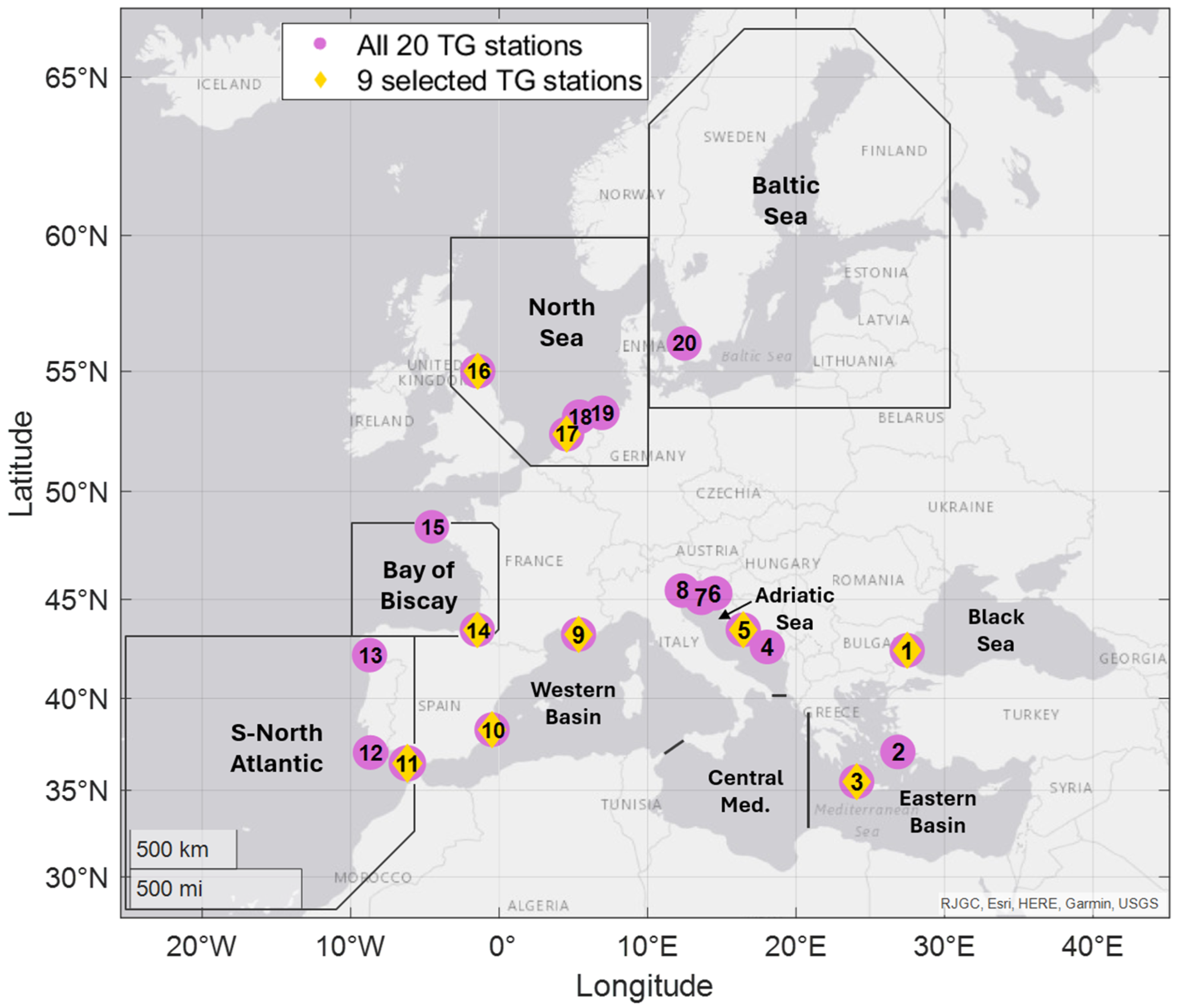
2.1. Study Area

This study examines the European seas region between latitudes 25° and 70° North and longitudes 25° West and 43° East, as shown in Figure 1. The region is comprised of 10 primary sub-regions: the Black Sea, the Mediterranean Sea (eastern, central, and western basins, and the Adriatic Sea), the South-North Atlantic Ocean, the Bay of Biscay, the North Sea, and the Baltic Sea.

2.2. Data Description

2.2.1. Sea Level Data

Tide-Gauge Data: This study utilizes monthly Revised Local Reference (RLR) data obtained from 20 TG stations along the European coast (see Figure 1), as provided by the Permanent Service for Mean Sea Level (https://psmsl.org/). The data and information for the sites were provided by the PSMSL, as detailed in Holgate et al. (2013) [31]. The dataset covers a period of over 45 years and exhibits a completeness rate exceeding 82%. The data was downloaded on 3 July 2023. Gaps in the dataset of more than two years were excluded from the study, while gaps of less than two years were linearly interpolated. For anomaly analysis, both mean and linear trends were removed from the data. No correction has been applied to the data, including the inverse barometer (IB) correction, which should not affect long-period variations such as those studied here. It is important to note that the interpolation method applied does not affect the results, as the filter we will apply later eliminates all frequencies below five years. Moreover, nine representative TG stations were carefully selected to ensure a well-balanced geographic distribution across the entire area. The stations selected for analysis, indicated by yellow diamonds in Figure 1, were chosen based on their geographic location and subsequent results.

Satellite Altimetry Data: This study uses the SL anomalies monthly maps for the European region (latitude from 25° to 70° north and longitude from 25° west to 43° east), covering the time interval from January 1993 to July 2022. These maps were derived from multi-mission altimetric satellites (Jason-3, Sentinel-3A, HY-2A, Saral/AltiKa, Cryosat-2, Jason-2, Jason-1, T/P, ENVISAT, GFO, ERS1/2) with a spatial resolution of 0.25° in a regular grid. The data were obtained from the Copernicus Climate Change Services (C3S, https://cds.climate.copernicus.eu/cdsapp#!/dataset/satellite-sea-level-global?tab=overview/, accessed on 10 November 2023). The IB correction has been applied. However, there is no inconsistency with the TG data as the IB correction only affects the high frequencies, and we remove these signals before starting our analysis (see Section 3). The SL data are anomalies with respect to the mean sea surface for the period 1993–2012, estimated as a composite of SIO, CNES/CLS15, and DTU15 mean sea surfaces [32,33].

2.2.2. Climate Indices

To establish a connection between the identified recurring patterns in SL, and atmospheric influences with significant climate modes over the North Atlantic, we use monthly NAO and AMO indices provided by the National Oceanic and Atmospheric Administration (https://www.noaa.gov/). The monthly averaged datasets encompass the period from 1950 to 2022 (https://www.noaa.gov/, accessed on 3 July 2023).

The NAO is a mode that characterizes the atmospheric variability over the northern Atlantic Ocean, eastern North America, and western Europe. It is measured as the sea-level atmospheric pressure difference between the Subtropical (Azores) High from southern station Lisbon (Portugal) and the Subpolar Low from northern station Reykjavik (Iceland). This data has been obtained from https://www.cpc.ncep.noaa.gov/products/precip/CWlink/pna/nao.shtml, accessed on 3 July 2023. In addition, NAO influences Northern Hemisphere surface temperatures and shows cyclical behavior with periods of 7, 13, 20, 26, and 34 years [34].

The AMO is the observed variability in the North Atlantic Ocean’s sea surface temperature (SST) over several decades. It is measured as fluctuations in the North Atlantic SST anomalies, 0–70°N. We used unsmoothed time series from https://psl.noaa.gov/data/timeseries/AMO/, accessed on 3 July 2023. The AMO alternates between positive and negative phases over periods of 65–70 years, affecting large-scale climate patterns [35].

2.3. Data Analysis Techniques

2.3.1. Hann Lowpass Filter

The Hann window is a mathematical function that tapers a segment of a time series in such a way as to reduce the influence of data points at the edges of the segment while emphasizing the central portion. A Hann window of length L (in our case is 60 months) is defined as follows:

$$H\left(n\right)=\{\begin{array}{c}0.5-0.5\cos \left({\displaystyle \frac{2\pi n}{L}}\right), 0\le n\le L-1, \\ 0 , \mathrm{otherwise}.\end{array}$$

(1)

The time series is filtered by convolving each segment of length L with the Hann window. The Hann filter was chosen for its ability to effectively mitigate spectral leakage and minimize abrupt discontinuities at signal edges by applying a smooth data tapering technique. The proposed method demonstrates an appropriate balance between frequency resolution and side lobe suppression, rendering it well-suited for scenarios that require accurate identification of frequency components while minimizing the disruption caused by neighboring spectral components. The Hann window exhibits desirable symmetry and amplitude scaling properties, allowing for effective signal smoothing and high-frequency reduction [36,37].

2.3.2. Temporal Correlation of Smoothed Time Series

Once the high frequencies have been filtered out, special care must be taken when calculating the significant levels of temporal correlations between time series. The temporal correlations and their significance levels are evaluated using a specific Monte Carlo analysis based on randomizing phases in the frequency domain [38]. In order to ascertain the significant level of the correlation between two different time series, a random time series is generated that has an identical power spectrum to the original time series but with a random phase. This process is repeated 1000 times to ensure statistical reliability. The generation of each of the 1000 random time series is achieved through three successive steps: (1) the discrete Fourier transform is computed for the given time series; (2) a new Fourier series is generated with random phases but with the power spectrum obtained in the previous step; (3) a new synthetic time series is derived by applying the inverse Fourier transform. The correlation between the other time series and the 1000 time series is then calculated. The level of significance is defined as the ratio of the correlation values exceeding the correlation value between the two original time series. This method is often used to assess the statistical significance of a calculated correlation coefficient in scenarios where serial correlation is a concern [38,39].

2.3.3. Wavelet Analysis

The WT is a widely used technique for performing time–frequency analysis, especially in oceanic data [40]. The Morlet wavelet is a particularly advantageous choice for continuous wavelet transform due to its ability to achieve an optimal balance between temporal and spectral localization, as evidenced by numerous studies [41,42,43,44,45]. The WT of a time series ${\left(x_n\right)}_{1\le n\le N}$ with uniform time steps $\delta t$ and without any gaps is defined as the convolution of $x_n$ with the normalized and scaled (by varying scaling $s$) wavelet mother ${\phi }_0$:

$$W_n^X\left(s\right)=\sqrt{{\displaystyle \frac{\delta t}{s}}} {\displaystyle \sum }_{i=1}^N{x}_i{\phi }_0\left[\left(i-n\right){\displaystyle \frac{\delta t}{s}}\right].$$

(2)

Another valuable measure is the coherence of the cross-wavelet transform in the time–frequency domain between two time series. The Wavelet Transform Coherence (WTC), which represents the degree of coherence between two time series, as defined in [42]:

$$R_n^2\left(s\right)={\displaystyle \frac{{\left|S\left(s^{-1}{W}_n^{XY}\left(s\right)\right)\right|}^2}{S\left(s^{-1}{\left|W_n^X\left(s\right)\right|}^2\right) · S\left(s^{-1}{\left|W_n^Y\left(s\right)\right|}^2\right)}} ,$$

(3)

where $S$ represents the smoothing operator and $W^{XY}=W^X{W}^{Y\ast }$, where $\ast$ represents the complex conjugation, and multiplication is a scalar product. This definition is similar to that of a traditional correlation coefficient, and it is helpful to consider that it is a localized correlation in the time–frequency domain.

Assuming a vertical slice through a wavelet transform plot represents the local spectrum, the time-averaged wavelet spectrum over all specified periods is the temporal mean of this spectrum and can be described as follows:

$$\overline{W^2}\left(s\right)={\displaystyle \frac{1}{N+1}}{\displaystyle \sum }_{i=1}^N{\left|W_i\left(s\right)\right|}^2.$$

(4)

where $N+1$ is the number of points in the time series [40].

The statistical significance level of the wavelet coherence is determined using Monte Carlo methods. An extensive ensemble of surrogate dataset pairs is generated to improve the dataset, ensuring that the AR1 (the first-order autoregressive process) coefficients of these surrogate datasets match those of the input datasets. The 5% significance level against the red noise is shown in the plots of WT and WTC with the thick outlined area. The directions of the arrows within the plots indicate the phase relationship between the two time series. In-phase is represented by an arrow pointing to the right, anti-phase by an arrow pointing to the left, and the first time series is ahead of the second one by a quarter of the cycle, represented by an arrow pointing straight down [42].

2.3.4. Multiresolution Wavelet Decomposition

In order to gain a comprehensive understanding of the underlying long-term frequencies present in SL time series and oceanic indices, it is essential to employ a frequency-based decomposition approach. Therefore, we used fixed-bandwidth and Multiresolution Wavelet Decomposition (MWD) analysis with nine-level decomposition to unravel the signals and extract the specific periodicities in the time series that are not accessible through the traditional Fourier transformation. In this paper, the original data is passed through a series of high- and low-wavelet decomposition filters using the Daubechies least-asymmetric wavelet with six vanishing moments, resulting in coarse-scale approximation coefficients and detail coefficients. Each detail coefficient (D1, D2, …, D9) is associated with a specific periodicity (the inverse of the corresponding frequency), and relative energy levels (the ratio of the wavelet coefficient’s energy at each level to the total energy) [46]. D1 is the component with the shortest periods (high frequency), while D9 is the component with the longest periods (low frequency). For additional details, please consult the Supplementary Materials, Figure S1, which shows the MWD of the Split TG station. For further details, please refer to [36,47].

The structure of this decomposition allows us to reassemble the components into the original signal, thereby preserving all the information. Our choice of wavelets is based on their adaptability to multiscale analysis and efficiency in capturing both short-term and long-term variations inherent in oceanic signals. This is due to their compact support and orthogonal basis, which is necessary for invertible decomposition using the discrete wavelet transform. For further details on the process, see [46,48].

The Morlet wavelet was employed for CWT and WTC since these methods are based on the continuous wavelet transform. The non-orthogonality and redundancy inherent to the Morlet wavelet facilitate smoother and more detailed time–frequency representations. In contrast, for MWD, which is based on discrete wavelet transforms, the Daubechies wavelet was selected due to its capacity to provide a compact support and an orthogonal basis, which are requisite for an invertible decomposition.

All data utilized in this study were processed using MATLAB, specifically version R2020b. The data analysis was conducted employing various MATLAB toolboxes, such as the Signal Processing Toolbox, Statistics and Machine Learning Toolbox, and Cross wavelet and wavelet coherence Toolbox by Aslak Grinsted [42], available at (https://github.com/grinsted/wavelet-coherence accessed on 3 July 2023).

3. Results

Since our focus is on SL variations rather than absolute values, we consider SL for both satellite altimetry and TG data. The altimetry data is provided as SL anomalies with respect to a reference surface obtained as a twenty-year mean period (1993–2012), using current altimeter standards (see Section 2.2.1). For each TG time series, SL data is provided as absolute SL. The anomalies to the mean for the period under study are considered, and the linear trend over the period is subtracted. The linear trends of the TG data, which are detailed in

Table 1. TG stations information and their linear trends (removed). The error in the linear trends is calculated by the standard deviation method.

Region	Station Name (Country)	Longitude	Latitude	Time Span (Length)	Completeness %	Trend ± Error (mm/Year)
Black Sea	1-Bourgas (Bulgari)	27.48	42.48	1950–1996 (46)	86	2.17 ± 0.56
Eastern basin	2-Leros (Greece)	26.85	37.13	1969–2022 (53)	83	1.86 ± 0.29
Eastern basin	3-Soudhas (Greece)	24.08	35.49	1969–2011 (42)	83	0.83 ± 0.45
Adriatic Sea	4-Dubrovnik (Croatia)	18.06	42.65	1956–2018 (62)	99	1.57 ± 0.27
Adriatic Sea	5-Split (Croatia)	16.44	43.51	1954–2018 (64)	87	1.03 ± 0.27
Adriatic Sea	6-Bakar (Croatia)	14.53	45.3	1950–2020 (70)	88	1.03 ± 0.27
Adriatic Sea	7-Rovinj (Croatia)	13.62	45.08	1955–2018 (63)	98	0.77 ± 0.30
Adriatic Sea	8-Venice (Italy)	12.33	45.43	1950–2000 (50)	94	1.23 ± 0.41
Western basin	9-Marseille (France)	5.35	43.28	1950–2022 (72)	96	1.07 ± 0.22
Western basin	10-Alicante (Spain)	−0.48	38.34	1960–2020 (60)	93	0.93 ± 0.21
S-North Atlantic	11-Cádiz (Spain)	−6.29	36.54	1961–2018 (57)	97	3.58 ± 0.30
S-North Atlantic	12-Lagos (Portugal)	−8.67	37.1	1950–1999 (49)	78	0.84 ± 0.38
S-North Atlantic	13-Vigo (Spain N)	−8.73	42.24	1950–2018 (68)	98	1.90 ± 0.27
Bay of Biscay	14-Boucau (France N)	−1.51	43.53	1967–2022 (55)	82	1.92 ± 0.39
Bay of Biscay	15-Brest (France N)	−4.49	48.38	1952–2022 (70)	90	2.07 ± 0.25
North Sea	16-North-Shield (UK)	−1.44	55.01	1950–2022 (72)	92	1.60 ± 0.17
North Sea	17-IJmuiden (Netherland)	4.55	52.46	1950–2021 (71)	100	1.90 ± 0.28
North Sea	18-Harlingen (Netherland)	5.41	53.18	1950–2021 (71)	100	1.85 ± 0.37
North Sea	19-Delfzijl (Netherland)	6.93	53.34	1950–2021 (71)	100	2.59 ± 0.37
Baltic Sea	20-Hornbaek (Danmark)	12.46	56.09	1950–2017 (67)	98	1.17 ± 0.34

, range from 0.77 ± 0.30 mm/year in Rovinj to 3.58 ± 0.30 mm/year in Cadiz. Additionally, there are no gaps in the time series because interpolation has been applied, enabling us to perform WT analysis.

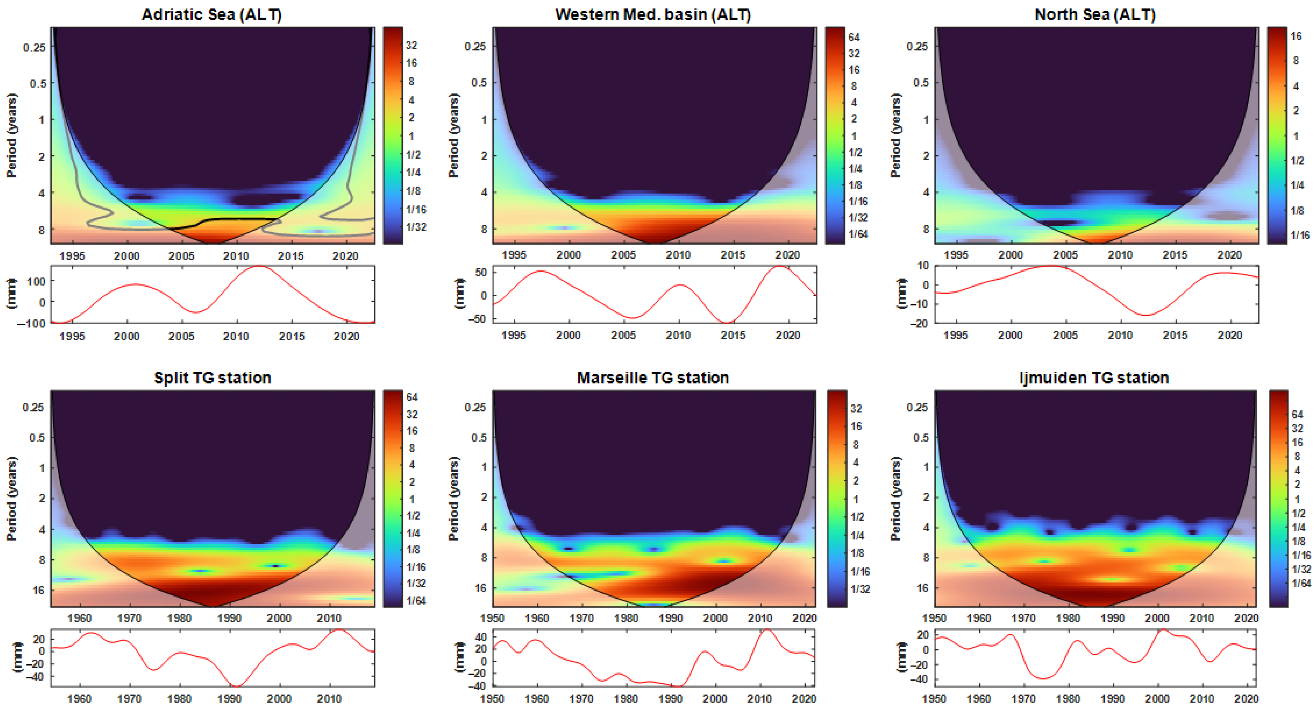
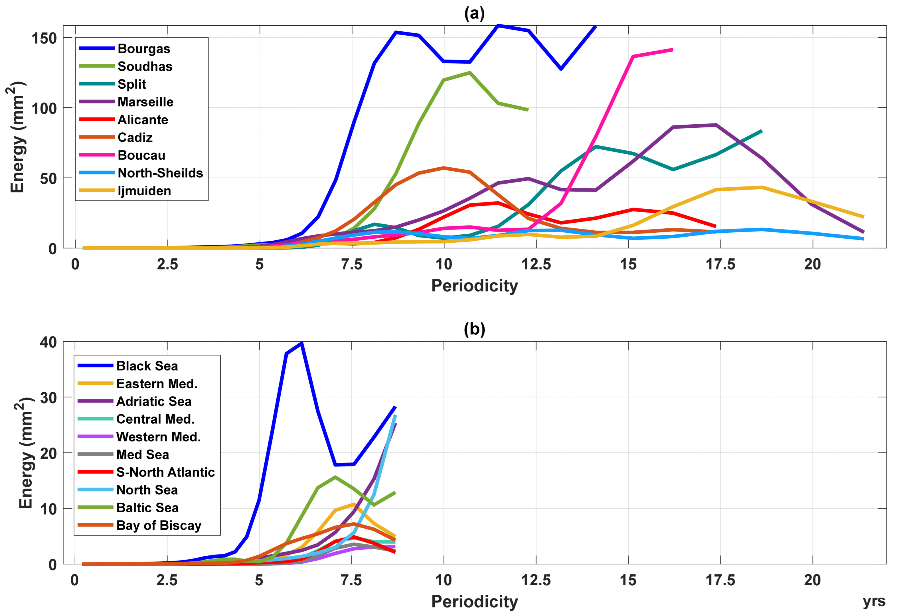
3.1. Unveiling Long-Term Periodicities in Sea Level

To identify and comprehend the long-term periodicities in SL, we first removed high frequencies below 5 years using the Hann filter (Section 2.3.2). Henceforth, we will refer to the filtered data as SL_HF, NAO_HF, and AMO_HF. Next, we applied WT to analyze the SL variability at different time scales and examine the changes in variance within the time–frequency domain of SL.

Figure 2 depicts the WT of SL_HF from three selected TG stations and altimetry data at their corresponding regions (see the Supplementary Materials to see them all in Figures S2 and S3). Most of the time series exhibit high power in the wavelet power spectrum at 6–8-year periods in altimetry time series, with increasing strength towards higher periodicities indicating the presence of long-term cycles. This pattern of cycles in SL is more evident in the power spectrum of the TG time series due to its longer time span. Here, we observe a prominent and strong band with a periodicity of around 8~20 years in most of the TG stations.

In Figure 3, the time-averaged wavelet spectrum is depicted using Equation (4). Figure 3a presents the energy distribution of SL_HF at nine TG stations (the selected TG stations are highlighted with yellow diamonds in Figure 1). Here, there is a variety of cycles in TG with periods ranging from 7 to 20 years with power magnitudes of 20 to 160 mm². In altimetry (Figure 3b), the periods range from 5 to 8.5 years, and the power is up to 40 mm². In some regions (such as the Black Sea, Western Mediterranean, North Sea, and Baltic Sea), the power seems to start increasing at about 8.5 years; however, the time series is too short to confirm this cycle. These results support and illustrate our previous findings in the WT, indicating the presence of long-term cycles in the SL.

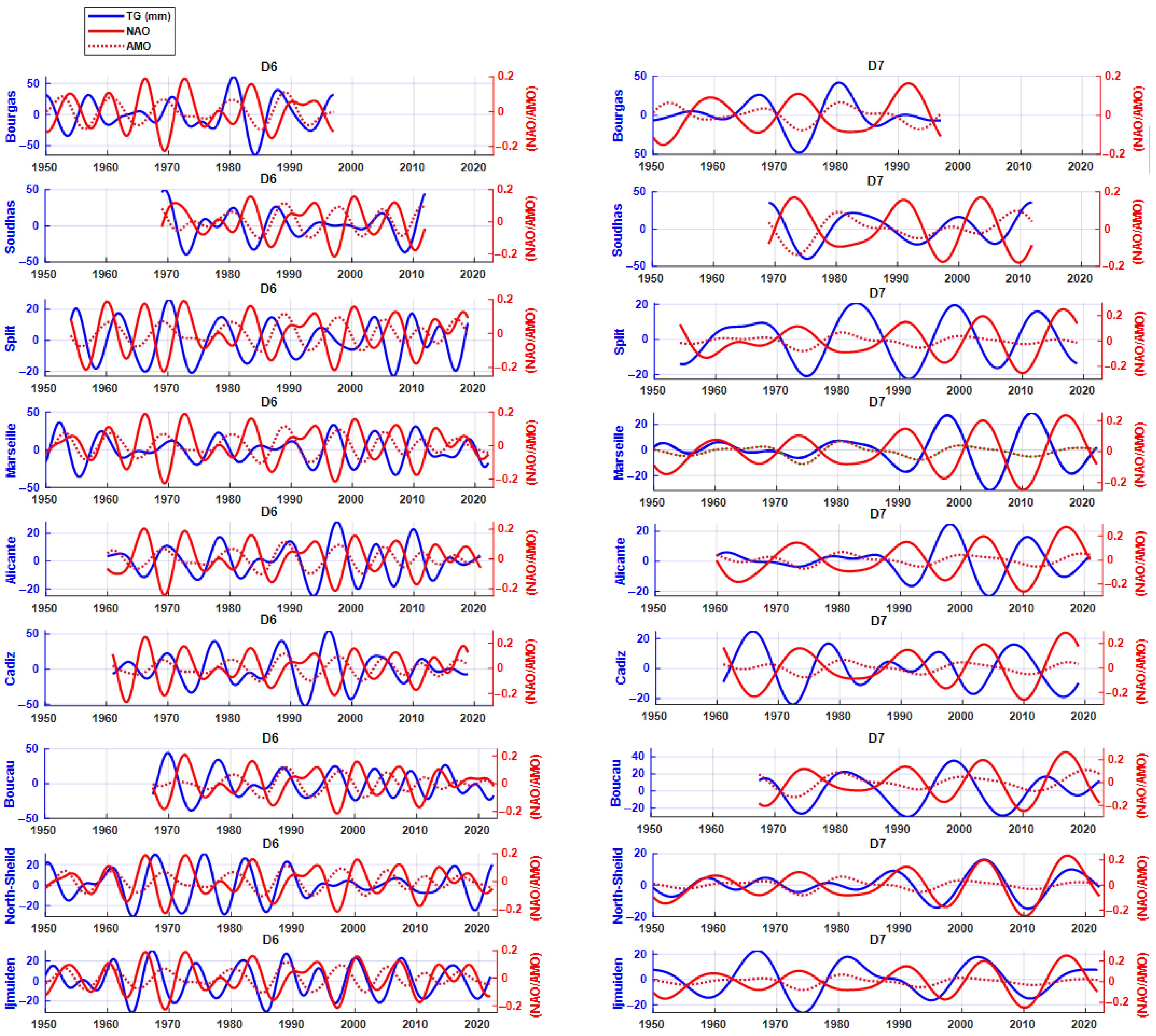
3.2. Multi-Resolution Analysis for Time–Frequency Domain and Connection with Indices

In order to analyze the long cycles that have been observed, it is crucial to first identify these periodic patterns. In this section, the observed SL data has been decomposed using MWD analysis (explained in Section 2.3.4). It is important to note that both the original and the Hann-filtered data showed a similar decomposition at low-frequency levels due to the effectiveness of the MWD in capturing frequencies. As a result, we chose to continue the decomposition with the original datasets to retain more information. A comprehensive demonstration of this decomposition applied to the detrended SL (no Hann filter applied) from the Split TG station is available in Supplementary Materials (Figure S1). This process provides valuable insight into the underlying dynamics of the SL periodicities.

Approximately 70% of the total energy of the original time series is concentrated in the first three components (D1, D2, and D3), which correspond to periods of one year or less (seasonality). In contrast, D6 and D7 correspond to periodicities of approximately 8 and 16 years, respectively, and account for between 2% and 6% of the total variance in SL from TG stations and around 2% and 7% in SL from altimetry in different regions. If we apply the decomposition to the SL_HF data, which has been filtered to exclude trends and periods of less than five years, the D6 and D7 components account for approximately 30% of the total variance at most TG stations.

To delve deeper into the primary influence of the SL at varying long cycles, we focused specifically on the D6 and D7 levels, which represent an approximately 8-year cycle (with a periodicity of 6 to 10 years), and a 16-year cycle (with a periodicity of 11 to 21 years), respectively, of the detrended SL, NAO, and AMO.

Figure 4 displays the D6 and D7 components derived from SL, NAO, and AMO indices from nine selected TG stations (the remaining stations are included in Figure S4 of the Supplementary Materials). A correlation pattern is observed during different time periods at both the 8 and 16-year scales. To further explore this idea, we calculate the correlations (as described in Section 2.3.2) between the SL_HF and the NAO_HF and AMO_HF indices, and between the corresponding D6 and D7 components.

Table 2. Temporal correlation between the spatial mean of studied regions of SL from altimetry and indices NAO and AMO for Hann-filtered, D6, and D7 time series with 90% significance (*: 95% significance level); the time period is 1993–2022.

Regions	Hann-Filtered Data		D6
	NAO	AMO	NAO	AMO
Black Sea		0.79 *	−0.62	0.92 *
Mediterranean Sea			−0.73 *
Eastern basin			−0.74 *
Central basin			−0.59
Adriatic Sea			−0.69 *
Western basin			−0.64 *
S-North Atlantic			−0.91 *
Bay of Biscay			−0.71 *
North Sea			−0.66 *
Baltic Sea		0.65 *

displays the temporal correlation between altimetry SL in the studied regions, as highlighted in Figure 1. Overall, a significant negative correlation is observed between the NAO index and D6, with the highest correlation coefficient reaching −0.91 in the South-North Atlantic. However, there is no significant correlation observed between SL and NAO at the D6 level in the Baltic Sea and the central Mediterranean Sea (see Supplementary Materials, Figure S5). Additionally, a robust positive correlation is evident with the AMO at the D7 level, exhibiting values between 0.87 and 0.96 in the Bay of Biscay, South-North Atlantic, and North Sea regions (not included in the table). However, one should be cautious when interpreting the results for D7 (~16 years cycle) in SL from altimetry, as the data set only extends to 29 years. Henceforth, we will analyze the SL from TG stations to obtain more significant results about long-term periodicities.

As evidenced in

Table 3. Temporal correlation table of SL from 20 TG stations with NAO and AMO indices of (Hann-filtered, D6, and D7 time series) with 90% significance, (*: 95% significance).

TG Stations	Hann-Filtered Data		D6		D7
	NAO	AMO	NAO	AMO	NAO	AMO
1-Bourgas			−0.51 *
2-Leros			−0.53 *		−0.67
3-Soudhas	−0.65 *			0.54		0.58
4-Dubrovnik	−0.74 *		−0.54 *			0.56
5-Split	−0.77 *		−0.50 *		−0.53	0.70 *
6-Bakar	−0.66 *		−0.42 *		−0.46	0.64
7-Rovinj	−0.71 *					0.56
8-Venice	−0.54				−0.84 *
9-Marseille	−0.64 *		−0.39	0.39	−0.77 *
10-Alicante	−0.66 *		−0.66 *	0.55 *	−0.76 *
11-Cádiz			−0.50 *	0.45	−0.72
12-Lagos
13-Vigo
14-Boucau			−0.50 *
15-Brest						0.76 *
16-North-Shield					0.77 *
17-IJmuiden		0.64 *	0.41 *			0.83 *
18-Harlingen			0.43		0.22
19-Delfzijl			0.30		0.22 *	0.77 *
20-Hornbaek		0.48 *

, the correlations between SL_HF and NAO_HF are strongly negative, with values ranging from −0.54 in Venice to −0.77 in Split. This anti-correlation was observed for the majority of TG stations located in the Mediterranean region. Conversely, SL_HF and AMO_HF showed positive correlations in northern Europe at IJmuiden and Hornbaek stations.

According to the results presented in Table 3, the correlation between the SL of the TG stations and the NAO at the D6 level shows a series of negative values in the region below 47° of latitude, with values ranging from −0.23 (Vigo) to −0.66 (Alicante), while Harlingen shows a positive correlation of 0.43 at the D6 level. This geographical pattern, which distinguishes negative from positive correlations, is well visualized in Figure 5a. At the D7 level, we notice a statistically significant positive correlation. Of particular note is the 0.84 negative correlation observed in Venice, which is statistically significant at the 95% level. Conversely, the TG stations located above 47° latitude show a positive correlation, reaching a value of 0.77 in North-Shields (95% significance).

The correlation between SL and AMO at both levels, D6 and D7, is predominantly positive. However, the significance levels vary (refer to Table 3), ranging from 0.39 in Marseille to 0.83 (95% significance) at the IJmuiden TG. Figure 5b provides a clear visualization of this correlation, indicating a geographic pattern where areas above 47° latitude exhibit notably higher significant positive correlations.

3.3. Time–Frequency Coherence of Sea Level and Atmospheric Indexes

Investigating the coherence in the time–frequency domain is an essential aspect of a comprehensive understanding of the influence of the ocean–atmosphere indices (NAO and AMO) and their connection to the observed long cycles in the SL. To achieve this, we applied the WTC approach explained in (Section 2.3.4) between the SL_HF time series and the indexes (NAO_HF and AMO_HF). The results are presented in Figure 6 and Figure 7, which show the SL_HF WTC with NAO_HF and SL_HF WTC with AMO_HF, respectively, at nine TG stations, which are highlighted with yellow diamonds in Figure 1 (the remaining stations are included in Supplementary Materials in Figures S6 and S7). The strong correlation observed at the edges and around the 0.25 period is negligible due to the absence of high frequencies in both time series caused by the application of the Hann filter with less than 5 years.

The analysis of the WTC of SL_HF and NAO_HF is depicted in Figure 6 and indicates a noteworthy 8-year cycle observed in most TG stations. Particularly, in the Mediterranean region (including Bourgas, Soudhas, Split, Venice, Boucau, and Cadiz), a distinct anti-correlation pattern, denoted by leftward-pointing arrows, is noticeable from 1960 to 2010, extending up to 2020 in stations such as Bakar, Marseille, Alicante, and Vigo. In contrast, along the North Sea (North Shield, IJmuiden, Harlingen, Delfzijl), it is evident that NAO led SL by approximately 2 years, as indicated by upward-pointing arrows, from 1950 to 1970. In addition, a 16-year cycle with significant anti-correlation phases (−0.65 to −0.85) can be observed from 1960 to 2020 over many Mediterranean regions (including Leros, Dubrovnik, Split, Rovinj, Venice, Marseille, Alicante, and Cadiz). This cycle is mainly observed at the North Shield station along the North Atlantic coast, with the NAO leading the SL by 4 years from 1980 to 2020.

Figure 7 depicts the WTC of AMO_HF and SL_HF, revealing a notable in-phase relationship with a periodicity of 8 to 14 years in most of the TG stations (including Bakar, Soudhas, Split, Marseille, Alicante, Cádiz, Vigo, Brest, Boucau, IJmuiden, and Hornbeak) with high values ranging from 0.65 to 0.90, spanning the period from the 1960s and 1970s until 2020. Furthermore, a robust and statistically significant 16-year cycle was observed across most of the stations studied on the Mediterranean coast, particularly in those located on the Adriatic and North European Seas.

Table 4. Temporal correlation between SL_HF, D6, D7, NAO, and AMO in the stations with high correlation periods detected from WTC with high coherence with 90% significance (*: 95% significance).

TG Stations	Periods		Hann-Filtered Data		D6		D7
	NAO	AMO	NAO	AMO	NAO	AMO	NAO	AMO
1-Bourgas	1978–1996	1965–1996			−0.72 *	0.71 *		0.81 *
	1965–1985	1965–1985					−0.93 *	0.91 *
6-Bakar	1965–2020	1980–2010		−0.52 *	−0.50 *			0.70 *
	1970–2000	X					−0.92 *
8-Venice	1970–2000	1970–2000	−0.90 *		−0.55 *			0.90 *
9-Marseille	1970–2021	1950–1995	−0.56 *		−0.58 *			−0.83 *
10-Alicante	X	1960–2000				0.66
11-Cadiz	1961–2010	1961–2010			−0.51 *			−0.67 *
13-Vigo	1980–2018	1970–2010			−0.34
	1980–2000	X					−0.91 *
14-Boucau	1967–2010	1985–2005	−0.54 *		−0.62 *
15-Brest	X	1952–1980
16-North-Shield	1980–2021	X					−0.85

presents the correlation between the SL and indexes at different levels (Hann-filtered, D6, and D7) during periods with high power, as observed previously in the WTC. To ensure the integrity of the analysis, we excluded the stations Leros, Soudhas, Dubrovnik, Split, Rovinj, IJmuiden, Harlingen, Delfzijl, and Hornbaek because they exhibited high correlation consistently throughout the entire period. Moreover, it is noteworthy that the Lagos station did not exhibit any significant coherence.

It can be observed that there is a common period for the correlation with NAO, with 8- and 16-year cycles. This observed correlation initiates from the decades of the 1960s and 1980s and persists to the years 2010 and 2020, respectively. Additionally, a significant correlation is observed in the Mediterranean Sea, with negative values up to −0.93.

Furthermore, the Time Dependent Temporal Correlation (TDTC) analysis between SL and NAO at the D6 level and SL and AMO at the D7 level (see Supplementary Materials for the TDTC methodology description and results in Figures S8–S11) supports this amalgamated correlation period noticed in WTC analysis. The results at the D6 level show a strong negative correlation between SL and NAO in absolute value over 0.88 in most TG stations across the Mediterranean Sea for the periods 1970–1990 and 1985–2020. On the other hand, TDTC results at the D7 level of SL and AMO show a strong positive correlation, reaching up to 0.90 for the periods 1960–1990 and 1970–2010 at most TG stations in the North Sea.

4. Discussion

This research analyzed long-term periodicities in SL from altimetry and TG stations through wavelet transform and multiresolution wavelet decomposition. Our primer results of the removed trends align with previous research [29,35,36,37]. Additionally, the WT and Averaged WT results showed that SL experienced long periodicities ranging from 8 to 20 years all along the European seas, which is similar to previous studies [49], where different periodicities were identified along the northern European coastline, including locations such as Brest, Delfzijl, IJmuiden, Hornbaek, North Shields, Harlingen, and other areas in the Netherlands. Despite anthropogenic changes in the 20th century, such as dredging near Delfzijl and the closure of the Zuiderzee [50], which significantly impacted fluvial and coastal systems, these periodicities have not been altered. The closure of the Zuiderzee in 1932 led to increased tidal range and current velocities in the Dutch Wadden Sea, while dredging activities in harbors and shipping lanes contributed to water turbidity [51].

Furthermore, the application of the Ensemble Empirical Mode Decomposition technique on SL, as presented in [10], revealed a dynamic oscillation in the SL tide gauge data of the Adriatic Sea, with a period of approximately 20 years. This oscillation was linked to the recurring opposite phases in the AMO and NAO. Furthermore, the significant fluctuations observed in SL in 2010 and 2011 were related to this long cycle pattern. Further investigation of annual precipitation in the Turkey region [29] revealed the presence of inter-decadal periodicities (8- and 16-year cycles). Importantly, these cycles do not exhibit a distinct geographical pattern.

The geographic pattern observed in the SL-AMO relationship may potentially be correlated with the sea surface temperature (SST) anomalies related to shifts in AMO, particularly during its negative phase, which spanned from 1964 to 1993. A study conducted by Zampieri et al. [52] demonstrated that during the negative phase of the AMO, sea level pressure exhibited a negative pattern over the British Isles. In contrast, a positive pattern was primarily observed over northeastern Europe. The AMO teleconnection over Europe has been found to significantly influence the alteration of frequencies of specific weather regimes due to the phase changing of the AMO [52].

The previously observed geographic and temporal patterns of the NAO-SL relationship may be attributed to the delayed response of the North Atlantic circulation to a surface heat flux force associated with the interdecadal variability of the NAO index. As evidenced by studies such as [53,54,55,56], there has been a notable eastward shift in the action centers of the NAO during the periods of intensified background flow between 1958–1977 and 1978–1997. This shift has been linked to the positioning of low-frequency intra-seasonal teleconnection patterns influenced by the diffluent part of the jet stream. It also coincided with significant changes in NAO-related climate variability, including changes in the Siberian wintertime temperature, sea ice export through Fram Strait, North Atlantic storm activity, and net surface heat fluxes in the North Atlantic region. Consequently, in [57], it has been proposed that the eastward shift of the NAO in the late 1970s may be associated with increased greenhouse gas concentrations, a heightened NAO index, and increased North Atlantic storm activity.

Furthermore, the strong correlation patterns of NAO and SL at 8- and 16-years level periodicities reported in our study may be caused by the significant decadal shifts in the indices, as evidenced by a positive correlation between the NAO zonal shift indices and the mean westerly winds over the North Atlantic region (50°–70°N) reported by Zhang et al. [57]. In addition, other studies have revealed a 10.5-year variability in SL along the northern European coast [21]. This variability was linked to significant decadal shifts in the NAO index and the intensity changes in Meridional Overturning Circulation and the heat transport in the area. These shifts impacted the entire North Atlantic Ocean and the Bay of Biscay. Additionally, the NAO decadal shifts could alter wind patterns associated with sea level pressure gradients over semi-enclosed seas, resulting in fluctuations in mass transport. This phenomenon has been observed in the Mediterranean, North, and Baltic Seas [58,59].

5. Conclusions

In this study, the empirical wavelet transform multiresolution analysis and continuous wavelet transform techniques were employed to analyze the SL data around Europe. The dataset encompasses 20 TG stations along the European coastline from 1950 to 2022, and SL from satellite altimetry data in nine different regions for the period 1993–2022. The main goal of the study was to explore the long-term periodicities of the European seas and understand their driving mechanisms. Key findings include:

• A multi-scale periodicity was observed using wavelet transform on SL data from the explored TG stations and regions from SL altimetry. This is characterized by two main low-frequency cycles: an 8-year cycle from altimetry data and longer cycles ranging from 8 to 18 years from TG data.
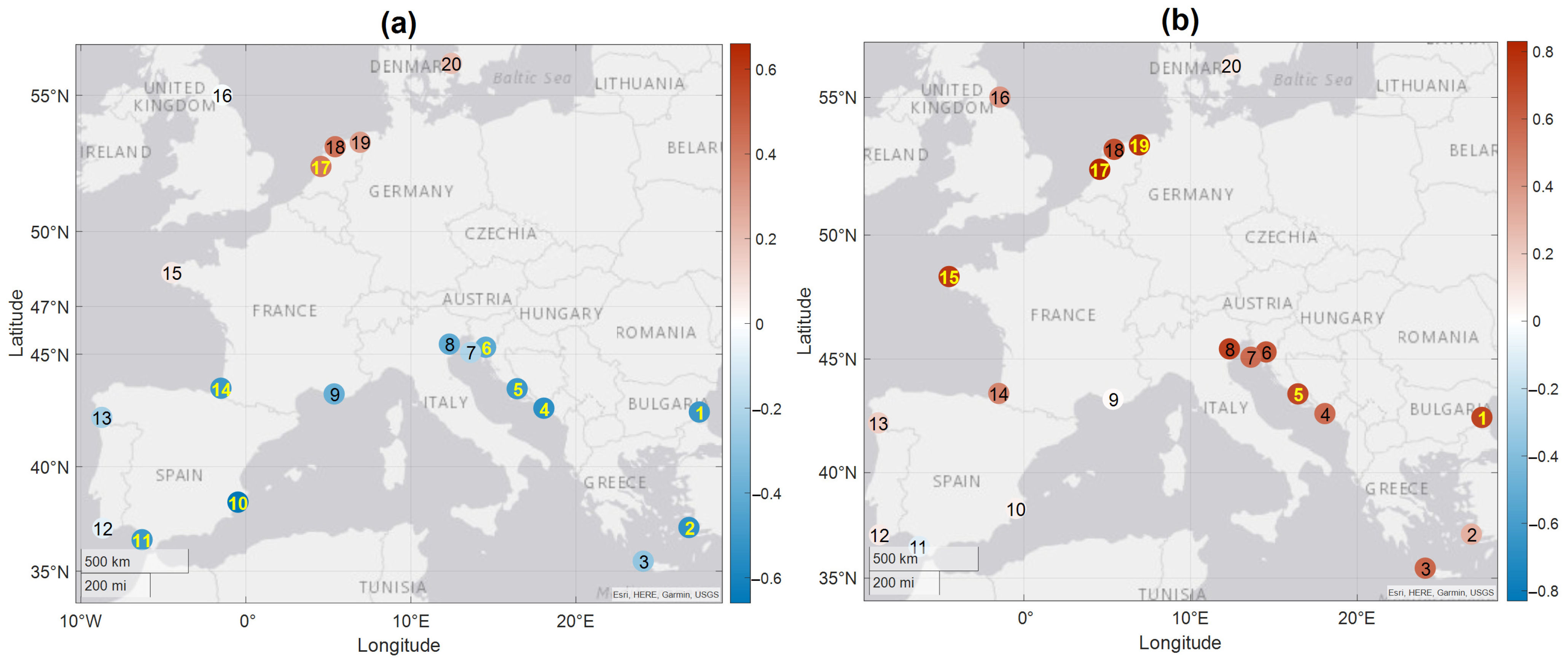
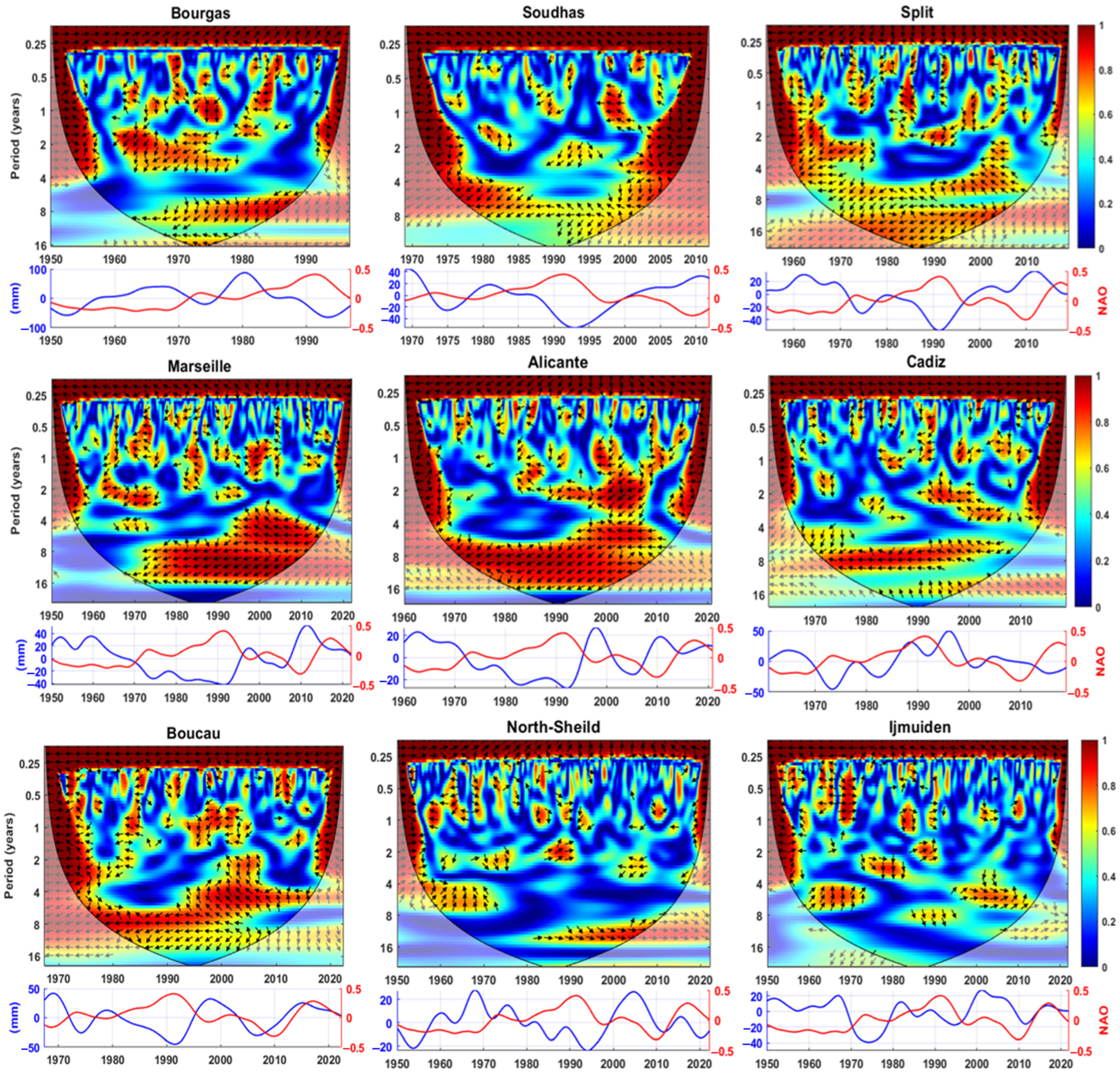
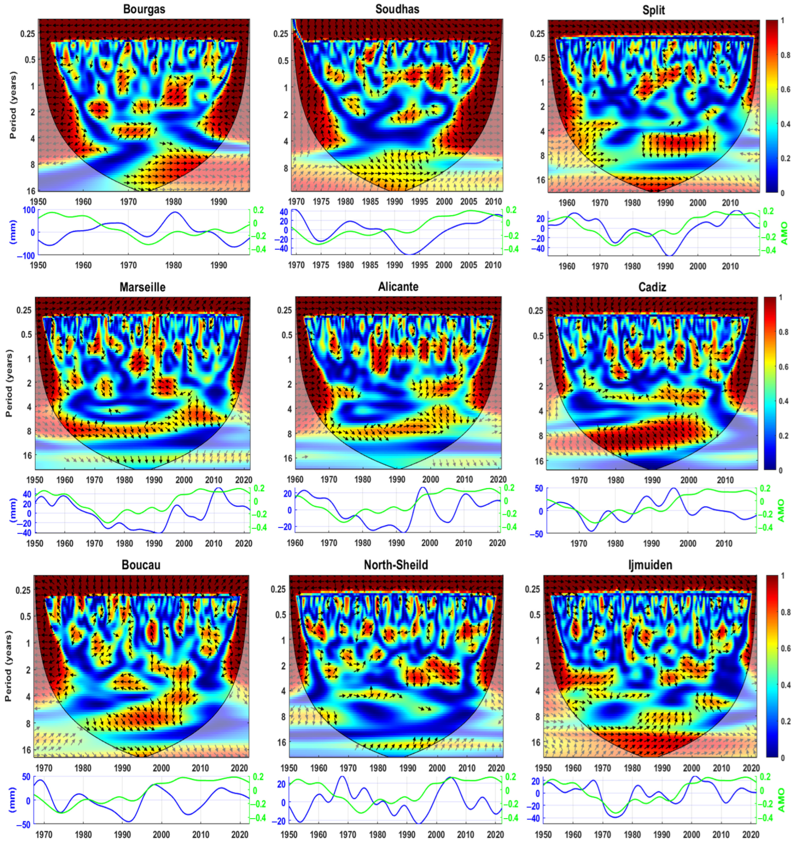
• The wavelet decomposition highlighted a significant correlation of the SL periodicity with the NAO and the AMO. Specifically, the NAO was identified as a critical factor influencing the 8-year cycle in SL, showing a negative correlation along the Mediterranean coast with values up to −0.66 in Alicante, and a positive moderate correlation within the northern European coast (above 47°N of latitude) with values reaching 0.43 in Harlingen station. Conversely, the AMO was more influential in the 16-year cycle, exhibiting a strong positive correlation up to 0.83 in IJmuiden, particularly in the northern studied areas.
• Further examination of the relationship with these climatic indices through Time Dependent Temporal Correlation highlighted significant periods during 1970–2010, 1970–1990, and 1985–2020, in which SL was greatly influenced by the NAO. This was characterized by a high correlation, approaching −0.90 along the Mediterranean Sea. Additionally, a strong positive correlation at the level of a 16-year cycle, reaching 0.90, was predominantly observed in the periods 1960–1990 and 1970–2010 in most TG stations located in the Mediterranean and North Seas, indicating a significant impact of the AMO on SL.

These findings offer valuable insights into the complex relationship between climatic indices and SL dynamics. They emphasize the necessity of elucidating the underlying mechanisms driving long-term sea level variations. Such knowledge has significant implications for coastal management, climate modeling and prediction, and adaptation strategies in the context of ongoing climate change.

References

1. Church, J.A.; White, N.J. Sea-Level Rise from the Late 19th to the Early 21st Century. Surv. Geophys. 2011, 32, 585–602. [Google Scholar] [CrossRef]
2. Cazenave, A.; Llovel, W. Contemporary Sea Level Rise. Ann. Rev. Mar. Sci. 2010, 2, 145–173. [Google Scholar] [CrossRef] [PubMed]
3. Melet, A.; van de Wal, R.; Amores, A.; Arns, A.; Chaigneau, A.A.; Dinu, I.; Haigh, I.D.; Hermans, T.H.J.; Lionello, P.; Marcos, M.; et al. Sea Level Rise in Europe: Observations and Projections. State Planet. Discuss. 2023, 2023, 1–106. [Google Scholar] [CrossRef]
4. Gower, J.; Barale, V. The Rising Concern for Sea Level Rise: Altimeter Record and Geo-Engineering Debate. Remote Sens. 2024, 16, 262. [Google Scholar] [CrossRef]
5. Rietbroek, R.; Brunnabend, S.-E.; Kusche, J.; Schröter, J.; Dahle, C. Revisiting the Contemporary Sea-Level Budget on Global and Regional Scales. Proc. Natl. Acad. Sci. USA 2016, 113, 1504–1509. [Google Scholar] [CrossRef] [PubMed]
6. Llovel, W.; Balem, K.; Tajouri, S.; Hochet, A. Cause of Substantial Global Mean Sea Level Rise Over 2014–2016. Geophys. Res. Lett. 2023, 50, e2023GL104709. [Google Scholar] [CrossRef]
7. Hooijer, A.; Vernimmen, R. Global LiDAR Land Elevation Data Reveal Greatest Sea-Level Rise Vulnerability in the Tropics. Nat. Commun. 2021, 12, 3592. [Google Scholar] [CrossRef]
8. Levermann, A.; Clark, P.U.; Marzeion, B.; Milne, G.A.; Pollard, D.; Radic, V.; Robinson, A. The Multimillennial Sea-Level Commitment of Global Warming. Proc. Natl. Acad. Sci. USA 2013, 110, 13745–13750. [Google Scholar] [CrossRef]
9. Strauss, B.H.; Kulp, S.A.; Rasmussen, D.J.; Levermann, A. Unprecedented Threats to Cities from Multi-Century Sea Level Rise. Environ. Res. Lett. 2021, 16, 114015. [Google Scholar] [CrossRef]
10. Galassi, G.; Spada, G. Linear and Non-Linear Sea-Level Variations in the Adriatic Sea from Tide Gauge Records (1872-2012). Ann. Geophys. 2015, 57, P0658. [Google Scholar] [CrossRef]
11. Dara Nur Arifin, A.; Taqyuddin, T. A Phenomenology Approach to Rethinking Coastal Community Vulnerability Toward Sea-Level Rise. Int. J. Soc. Health 2023, 2, 345–353. [Google Scholar] [CrossRef]
12. Srinivasan, M.; Tsontos, V. Satellite Altimetry for Ocean and Coastal Applications: A Review. Remote Sens. 2023, 15, 3939. [Google Scholar] [CrossRef]
13. Lumban-Gaol, J.; Sumantyo, J.T.S.; Tambunan, E.; Situmorang, D.; Antara, I.M.O.G.; Sinurat, M.E.; Suhita, N.P.A.R.; Osawa, T.; Arhatin, R.E. Sea Level Rise, Land Subsidence, and Flood Disaster Vulnerability Assessment: A Case Study in Medan City, Indonesia. Remote Sens. 2024, 16, 865. [Google Scholar] [CrossRef]
14. Fernández-Montblanc, T.; Gómez-Enri, J.; Ciavola, P. The Role of Mean Sea Level Annual Cycle on Extreme Water Levels Along European Coastline. Remote Sens. 2020, 12, 3419. [Google Scholar] [CrossRef]
15. Passeri, D.L.; Hagen, S.C.; Medeiros, S.C.; Bilskie, M.V.; Alizad, K.; Wang, D. The Dynamic Effects of Sea Level Rise on Low-gradient Coastal Landscapes: A Review. Earths Future 2015, 3, 159–181. [Google Scholar] [CrossRef]
16. Kirwan, M.L.; Megonigal, J.P. Tidal Wetland Stability in the Face of Human Impacts and Sea-Level Rise. Nature 2013, 504, 53–60. [Google Scholar] [CrossRef] [PubMed]
17. Garcia-Soto, C.; Cheng, L.; Caesar, L.; Schmidtko, S.; Jewett, E.B.; Cheripka, A.; Rigor, I.; Caballero, A.; Chiba, S.; Báez, J.C.; et al. An Overview of Ocean Climate Change Indicators: Sea Surface Temperature, Ocean Heat Content, Ocean PH, Dissolved Oxygen Concentration, Arctic Sea Ice Extent, Thickness and Volume, Sea Level and Strength of the AMOC (Atlantic Meridional Overturning Circulation). Front. Mar. Sci. 2021, 8, 642372. [Google Scholar] [CrossRef]
18. Jevrejeva, S.; Grinsted, A.; Moore, J.C.; Holgate, S. Nonlinear Trends and Multiyear Cycles in Sea Level Records. J. Geophys. Res. Ocean. 2006, 111. [Google Scholar] [CrossRef]
19. Agha Karimi, A.; Deng, X.; Andersen, O.B. Sea Level Variation around Australia and Its Relation to Climate Indices. Mar. Geod. 2019, 42, 469–489. [Google Scholar] [CrossRef]
20. Tsimplis, M.N.; Calafat, F.M.; Marcos, M.; Jordà, G.; Gomis, D.; Fenoglio-Marc, L.; Struglia, M.V.; Josey, S.A.; Chambers, D.P. The Effect of the NAO on Sea Level and on Mass Changes in the Mediterranean Sea. J. Geophys. Res. Ocean. 2013, 118, 944–952. [Google Scholar] [CrossRef]
21. Iglesias, I.; Lorenzo, M.N.; Lázaro, C.; Fernandes, M.J.; Bastos, L. Sea Level Anomaly in the North Atlantic and Seas around Europe: Long-Term Variability and Response to North Atlantic Teleconnection Patterns. Sci. Total Environ. 2017, 609, 861–874. [Google Scholar] [CrossRef] [PubMed]
22. Scafetta, N. Multi-Scale Dynamical Analysis (MSDA) of Sea Level Records versus PDO, AMO, and NAO Indexes. Clim. Dyn. 2014, 43, 175–192. [Google Scholar] [CrossRef]
23. Ozgenc Aksoy, A. Investigation of Sea Level Trends and the Effect of the North Atlantic Oscillation (NAO) on the Black Sea and the Eastern Mediterranean Sea. Theor. Appl. Clim. 2017, 129, 129–137. [Google Scholar] [CrossRef]
24. Jevrejeva, S.; Moore, J.C.; Woodworth, P.L.; Grinsted, A. Influence of Large-Scale Atmospheric Circulation on European Sea Level: Results Based on the Wavelet Transform Method. Tellus A Dyn. Meteorol. Oceanogr. 2005, 57, 183. [Google Scholar] [CrossRef]
25. Bonaduce, A.; Pinardi, N.; Oddo, P.; Spada, G.; Larnicol, G. Sea-Level Variability in the Mediterranean Sea from Altimetry and Tide Gauges. Clim. Dyn. 2016, 47, 2851–2866. [Google Scholar] [CrossRef]
26. Wakelin, S.L.; Woodworth, P.L.; Flather, R.A.; Williams, J.A. Sea-level Dependence on the NAO over the NW European Continental Shelf. Geophys. Res. Lett. 2003, 30, e2003GL017041. [Google Scholar] [CrossRef]
27. Tantet, A.; Dijkstra, H.A. An Interaction Network Perspective on the Relation between Patterns of Sea Surface Temperature Variability and Global Mean Surface Temperature. Earth Syst. Dyn. 2014, 5, 1–14. [Google Scholar] [CrossRef]
28. Hansen, J.M.; Aagaard, T.; Kuijpers, A. Sea-Level Forcing by Synchronization of 56- and 74-Year Oscillations with the Moon’s Nodal Tide on the Northwest European Shelf (Eastern North Sea to Central Baltic Sea). J. Coast. Res. 2015, 315, 1041–1056. [Google Scholar] [CrossRef]
29. Partal, T. Wavelet Based Periodical Analysis of the Precipitation Data of the Mediterranean Region and Its Relation to Atmospheric Indices. Model. Earth Syst. Environ. 2018, 4, 1309–1318. [Google Scholar] [CrossRef]
30. Liang, X.; Lin, Y.; Wu, R.; Li, G.; Khan, N.; Liu, R.; Su, H.; Wei, S.; Zhang, H. Time-Frequency Analysis Framework for Understanding Non-Stationary and Multi-Scale Characteristics of Sea-Level Dynamics. Front. Mar. Sci. 2023, 9, 1070727. [Google Scholar] [CrossRef]
31. Holgate, S.J.; Matthews, A.; Woodworth, P.L.; Rickards, L.J.; Tamisiea, M.E.; Bradshaw, E.; Foden, P.R.; Gordon, K.M.; Jevrejeva, S.; Pugh, J. New Data Systems and Products at the Permanent Service for Mean Sea Level. J. Coast. Res. 2013, 29, 493–504. [Google Scholar] [CrossRef]
32. Pujol, M.; Schaeffer, P.; Faugère, Y.; Raynal, M.; Dibarboure, G.; Picot, N. Gauging the Improvement of Recent Mean Sea Surface Models: A New Approach for Identifying and Quantifying Their Errors. J. Geophys. Res. Ocean. 2018, 123, 5889–5911. [Google Scholar] [CrossRef]
33. Sandwell, D.T.; Harper, H.; Tozer, B.; Smith, W.H.F. Gravity Field Recovery from Geodetic Altimeter Missions. Adv. Space Res. 2021, 68, 1059–1072. [Google Scholar] [CrossRef]
34. Seip, K.L.; Grøn, Ø.; Wang, H. The North Atlantic Oscillations: Cycle Times for the NAO, the AMO and the AMOC. Climate 2019, 7, 43. [Google Scholar] [CrossRef]
35. Hernández, A.; Sáez, A.; Bao, R.; Raposeiro, P.M.; Trigo, R.M.; Doolittle, S.; Masqué, P.; Rull, V.; Gonçalves, V.; Vázquez-Loureiro, D.; et al. The Influences of the AMO and NAO on the Sedimentary Infill in an Azores Archipelago Lake since ca. 1350 CE. Glob. Planet. Change 2017, 154, 61–74. [Google Scholar] [CrossRef]
36. Proakis, J.G.; Manolakis, D.G. Digital Signal Processing: Principles, Algorithms, and Applications; Pearson: London, UK, 2006. [Google Scholar]
37. Oppenheim, A.V.; Schafer, R.W. Discrete-Time Signal Processing; Pearson: London, UK, 2010. [Google Scholar]
38. Ebisuzaki, W. A Method to Estimate the Statistical Significance of a Correlation When the Data Are Serially Correlated. J. Clim. 1997, 10, 2147–2153. [Google Scholar] [CrossRef]
39. Macias-Fauria, M.; Grinsted, A.; Helama, S.; Holopainen, J. Persistence Matters: Estimation of the Statistical Significance of Paleoclimatic Reconstruction Statistics from Autocorrelated Time Series. Dendrochronologia 2012, 30, 179–187. [Google Scholar] [CrossRef]
40. Torrence, C.; Compo, G.P. A Practical Guide to Wavelet Analysis. In Bulletin of the American Meteorological Society; American Meteorological Society: Boston, MA, USA, 1998; pp. 61–78. [Google Scholar]
41. Kumar, P.; Foufoula-Georgiou, E. Wavelet Analysis for Geophysical Applications. Rev. Geophys. 1997, 35, 385–412. [Google Scholar] [CrossRef]
42. Grinsted, A.; Moore, J.C.; Jevrejeva, S. Application of the Cross Wavelet Transform and Wavelet Coherence to Geophysical Time Series. Nonlinear Process Geophys. 2004, 11, 561–566. [Google Scholar] [CrossRef]
43. Percival, D.B. Analysis of Geophysical Time Series Using Discrete Wavelet Transforms: An Overview. In Nonlinear Time Series Analysis in the Geosciences; Springer: Berlin/Heidelberg, Germany, 2008; pp. 61–79. [Google Scholar]
44. Zhang, K.; Gençay, R.; Ege Yazgan, M. Application of Wavelet Decomposition in Time-Series Forecasting. Econ. Lett. 2017, 158, 41–46. [Google Scholar] [CrossRef]
45. Erol, S. Time-Frequency Analyses of Tide-Gauge Sensor Data. Sensors 2011, 11, 3939–3961. [Google Scholar] [CrossRef] [PubMed]
46. Percival, D.B.; Walden, A.T. Wavelet Methods for Time SeriesAnalysis; Cambridge University Press: Cambridge, MA, USA, 2000; ISBN 9780511841040. [Google Scholar]
47. Akansu, A.N.; Haddad, R.A. Multiresolution Signal Decomposition: Transforms, Subbands, and Wavelets, 2nd ed.; Academic Press: Cambridge, MA, USA; New Jersey Institute of Technology: Newark, NJ, USA, 2001. [Google Scholar]
48. Habimana, O. Wavelet Multiresolution Analysis of the Liquidity Effect and Monetary Neutrality. Comput. Econ. 2019, 53, 85–110. [Google Scholar] [CrossRef]
49. Baker, R.G.V.; McGowan, S.A. Periodicities in Mean Sea-Level Fluctuations and Climate Change Proxies: Lessons from the Modelling for Coastal Management. Ocean. Coast. Manag. 2014, 98, 187–201. [Google Scholar] [CrossRef]
50. de Jonge, V.N.; Essink, K.; Boddeke, R. The Dutch Wadden Sea: A Changed Ecosystem. Hydrobiologia 1993, 265, 45–71. [Google Scholar] [CrossRef]
51. Surian, N. Fluvial Changes in the Anthropocene: A European Perspective. In Treatise on Geomorphology; Elsevier: Amsterdam, The Netherlands, 2022; pp. 561–583. [Google Scholar]
52. Zampieri, M.; Toreti, A.; Schindler, A.; Scoccimarro, E.; Gualdi, S. Atlantic Multi-Decadal Oscillation Influence on Weather Regimes over Europe and the Mediterranean in Spring and Summer. Glob. Planet. Change 2017, 151, 92–100. [Google Scholar] [CrossRef]
53. Ulbrich, U.; Christoph, M. A Shift of the NAO and Increasing Storm Track Activity over Europe Due to Anthropogenic Greenhouse Gas Forcing. Clim. Dyn. 1999, 15, 551–559. [Google Scholar] [CrossRef]
54. Eden, C.; Jung, T. North Atlantic Interdecadal Variability: Oceanic Response to the North Atlantic Oscillation (1865–1997). J. Clim. 2001, 14, 676–691. [Google Scholar] [CrossRef]
55. Jung, T.; Hilmer, M.; Ruprecht, E.; Kleppek, S.; Gulev, S.K.; Zolina, O. Characteristics of the Recent Eastward Shift of Interannual NAO Variability. J. Clim. 2003, 16, 3371–3382. [Google Scholar] [CrossRef]
56. Nakamura, T.; Yamazaki, K.; Iwamoto, K.; Honda, M.; Miyoshi, Y.; Ogawa, Y.; Ukita, J. A Negative Phase Shift of the Winter AO/NAO Due to the Recent Arctic Sea-ice Reduction in Late Autumn. J. Geophys. Res. Atmos. 2015, 120, 3209–3227. [Google Scholar] [CrossRef]
57. Zhang, X.; Jin, L.; Chen, C.; Guan, D.; Li, M. Interannual and Interdecadal Variations in the North Atlantic Oscillation Spatial Shift. Chin. Sci. Bull. 2011, 56, 2621–2627. [Google Scholar] [CrossRef]
58. García-García, D.; Vigo, I.; Trottini, M. Water Transport among the World Ocean Basins within the Water Cycle. Earth Syst. Dyn. 2020, 11, 1089–1106. [Google Scholar] [CrossRef]
59. Boulahia, A.K.; García-García, D.; Vigo, M.I.; Trottini, M.; Sayol, J.-M. The Water Cycle of the Baltic Sea Region from GRACE/GRACE-FO Missions and ERA5 Data. Front. Earth Sci. 2022, 10, 879148. [Google Scholar] [CrossRef]
Figure 1. Study area. Locations of the tide gauge stations are marked with purple circles and numbered according to Table 1. The nine regions considered for altimetry data are delineated as black lines, with the corresponding names. The TG stations highlighted with yellow diamonds are the nine selected for display in the figures.
Remotesensing 16 02931 g001
Figure 2. Wavelet transform spectrum of SLHF, lower panel: from three TG stations (Split, Marseille and IJmuiden); upper panel: the corresponding mean regions from altimetry, all along with SLHF time series (red curve). The color bar represents the normalized variances (by 1/σ2).
Remotesensing 16 02931 g002
Figure 3. Time-Averaged Wavelet Spectrum: (a) SLHF from nine TG stations, (b) SLHF from altimetry in the nine studied regions. Selected TG stations are highlighted with yellow diamonds in Figure 1. The time series are time-averaged wavelet spectrum estimates as shown in Equation (4).
Remotesensing 16 02931 g003
Figure 4. D6 (left panels) and D7 (right panels) wavelet decompositions for sea level anomalies of nine TG stations (blue curves), NAO (dashed red curves), and AMO (dashed green curves). Selected TG stations are highlighted with a yellow diamond in Figure 1.
Remotesensing 16 02931 g004
Figure 5. Temporal correlation maps between: (a) D6 of SL and NAO, (b) D7 of SL and AMO. The color bar reflects the correlation value with a significance higher than 70%, and the highlighted yellow numbers represent the results with 95% significance.
Remotesensing 16 02931 g005
Figure 6. The lower panel represents two-time series SL from the TG stations (blue curve) and NAO index (red curve), both Hann-filtered, and the upper panel represents the WTC of both time series (SL from nine selected TG stations highlighted with yellow diamonds in Figure 1). The arrows represent the relative phase, with in-phase pointing right, anti-phase pointing left, and NAO leading SL by a quarter of the cycle pointing straight down.
Remotesensing 16 02931 g006
Figure 7. The lower panel represents two-time series SL from the TG stations (blue curve) and AMO index (green curve), both Hann-filtered, and the upper panel represents the WTC of both time series (SL from nine selected TG stations highlighted with yellow diamonds in Figure 1). The arrows represent the relative phase, with in-phase pointing right, anti-phase pointing left, and AMO leading SL by a quarter of the cycle pointing straight down.
Remotesensing 16 02931 g007