A Segmented Sliding Window Reference Signal Reconstruction Method Based on Fuzzy C-Means

Abstract

Reference signal reconstruction serves as a crucial technique for suppressing multipath interference and noise in the reference channel of passive radar. Aiming at the challenge of detecting Low-Slow-Small (LSS) targets using Digital Terrestrial Multimedia Broadcasting (DTMB) signals, this article proposes a novel segmented sliding window reference signal reconstruction method based on Fuzzy C-Means (FCM). By partitioning the reference signals based on the structure of DTMB signal frames, this approach compensates for frequency offset and sample rate deviation individually for each segment. Additionally, FCM clustering is utilized for symbol mapping reconstruction. Both simulation and experimental results show that the proposed method significantly suppresses constellation diagram divergence and phase rotation, increases the adaptive cancellation gain and signal-to-noise ratio (SNR), and in the meantime reduces the computation cost.

1. Introduction

In recent years, Low-Slow-Small (LSS) targets represented by Unmanned Aerial Vehicles (UAVs) have made full use of low-altitude flight capabilities [1]. They posed a threat to government agencies, airports, and important gatherings [2]. The major security risks had attracted worldwide attention. At present, the main detection means of LSS targets include radio detection equipment [3], photoelectric equipment [4], and radar [5]. The radio detection equipment detects targets by using the image transmission and telemetry signal of the UAV, but it is vulnerable to the interference of a complex electromagnetic environment [6]. The photoelectric equipment tracks targets through infrared and visible light; however, it is seriously affected by the weather [7,8]. Radar can work in all weather conditions and is the main method for target early warning and detection [9,10].

Due to the strong environment interference and small radar cross section of LSS targets [11], traditional radar has limited detection capabilities. Passive radar utilizes non-cooperative signals as illumination sources to achieve moving target detection and localization through coherent accumulation [12]. It is considered to be a potentially effective solution to the above challenges. Exploiting its inherent characteristic of not emitting radio waves, it eliminates the influence of radio interference and effectively avoids being detected and disrupted by enemy [13,14]. Compared with traditional radars, its excellent low-altitude coverage capabilities and easy deployment give it obvious advantages in detecting LSS targets [15,16]. However, the emission power and waveform parameters of illumination sources are uncontrollable [17]. Therefore, appropriate signals must be selected as radiation sources to ensure the detection performance of the system. Currently, research concerning the illumination sources of opportunity signals includes Digital Audio Broadcasting (DAB) [18,19,20], Digital Video Broadcasting-terrestrial (DVB-T) [21,22,23], Digital Terrestrial Multimedia Broadcasting signals (DTMB) [24,25,26], etc. The DTMB, characterized by wide signal bandwidth, high emission power, and extensive coverage, emerges as an ideal illumination source for passive radar [27].

A novel approach was utilized in target detection by simultaneously receiving target echo signals from the surveillance channel and reference signals from the reference channel in passive radar [28,29]. After the correlation processing of both channels, crucial target information such as distance, speed, and coordinates were extracted [30]. The reference signal serves two important purposes. Firstly, it contributes to clutter cancellation to suppress direct waves and clutter in the echo signals [31]. Secondly, it facilitates a coherent accumulation with the echo signals for target detection [32]. The effectiveness of interference suppression and the reliability of target detection were significantly influenced by the quality of the reference signal [33,34]. In practical scenarios, the reference signal included not only direct waves but also multipath interference and clutter caused by buildings and terrain during the transmission, which posed new challenges for signal reconstruction methods [35,36].

The time-domain reference signal reconstruction method was drawn on the signal demodulation techniques commonly used in communication systems [37]. Interference suppression in the reference channel was achieved, and non-coherent interference could be effectively suppressed [38]. However, considerable computational resources were consumed in the process of symbol reconstruction by adopting this method [39]. Additionally, errors may occur during the estimation of frequency offset and sample rate deviation, resulting in constellation diagram divergence and phase rotation [40]. Consequently, the bit error rate (BER) of the reconstructed signal was increased, thus reducing the interference suppression gain.

To address the issues of constellation diagram divergence and phase rotation, and reduce the computation cost of the reconstruction process, a segmented sliding window reference signal reconstruction method based on Fuzzy C-Means (FCM) is proposed in this paper. The proposed method compensates the frequency offset and sampling rate deviation, to solve the problems of constellation divergence and phase rotation caused by error accumulation. The FCM clustering is used in the symbol mapping reconstruction to reduce the computation cost.

The remainder of the paper is organized as follows. The DTMB standard is introduced in Section 2. The traditional reconstruction procedure is overviewed in Section 3, followed by a detailed description of the methods proposed in this article. In Section 4, the effectiveness of the proposed methods is verified by simulated and measured data. A relevant summary and conclusions are given in Section 5.

2. DTMB Standard

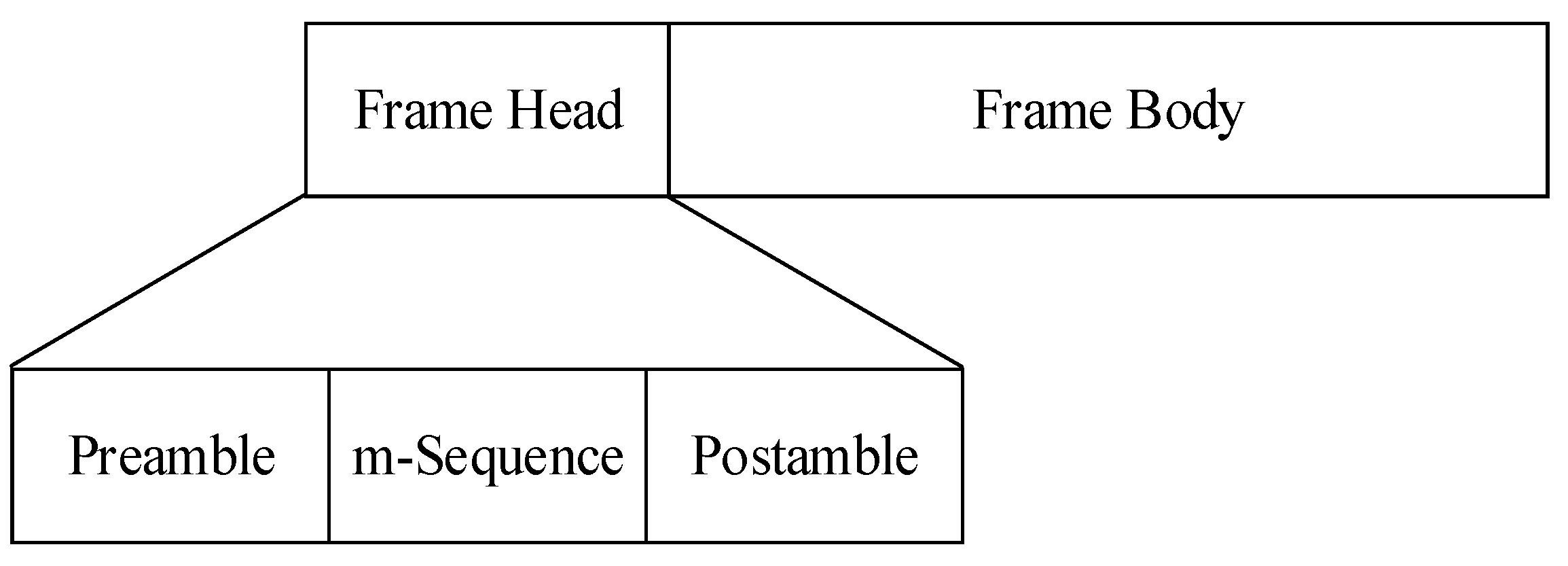
2.1. Signal Structure of DTMB

The DTMB standard, titled ‘Framing Structure, Channel Coding and Modulation for Digital Television Terrestrial Broadcasting System’, was announced in August 2006 [41]. This standard has independent intellectual property rights in China and is a mandatory national standard for digital televisions. The combination of Time-Domain Synchronous Orthogonal Frequency Division Multiplexing (TDS-OFDM) and LDPC (Low-density Parity-check) coding techniques is used in DTMB signals. In the core of the DTMB system structure, the signal frame is the basic unit. The frame structure of DTMB signals is shown in Figure 1. The frame structure contains two essential components, namely the frame head (FH) and the frame body (FB). The FB is comprised of 36 system information symbols and 3744 data symbols, totaling 3780 symbols. Meanwhile, the FH includes three variations: 420 or 945 symbols in the multi-carrier mode and 595 symbols in the single-carrier mode.

Taking PN420 mode as an example, the FH is composed of a preamble, an eighth-order PN sequence, and a postamble. Notably, the preamble and postamble are composed of the initial 83 symbols and the concluding 82 symbols of the m-sequence, respectively. A distinct PN sequence with different initial phases is used for each FH signal as a unique identification of the frame number. The linear feedback shift register of PN420 is shown in Figure 2.

For a multi-carrier with frame head PN420, the time-domain expression of the signal frame is shown in Equation (1), where $N_t$ and $N_c$ represent the symbol length of FH and FB, respectively; $PN(n)$ is frame head data; $k$ denotes the number of the carrier frequency; and $X(k)$ represents the FB symbol before modulation.

$$x(n)=\left\{\begin{array}{c}PN(n),n\in \left[0,N_t-1\right]\\ {\displaystyle \sum _{k=0}^{N_{\mathrm{c}}-1}X(k)\exp \left[\frac{j2\pi (n-N_t)k}{N_c}\right],n\in \left[N_t,N_t+N_c-1\right].}\end{array}\right.$$

(1)

2.2. Transmitting System Scheme

The DTMB transmission system completes the conversion from an input data stream to the transmission signal [42,43]. Figure 3 shows the transmitter block diagram, which consists of the following elements:

• randomization of the input data;
• forward error correction coding;
• mapping and interleaving;
• frame combination and baseband processing;
• orthogonal up-conversion.

3. Reference Signal Reconstruction

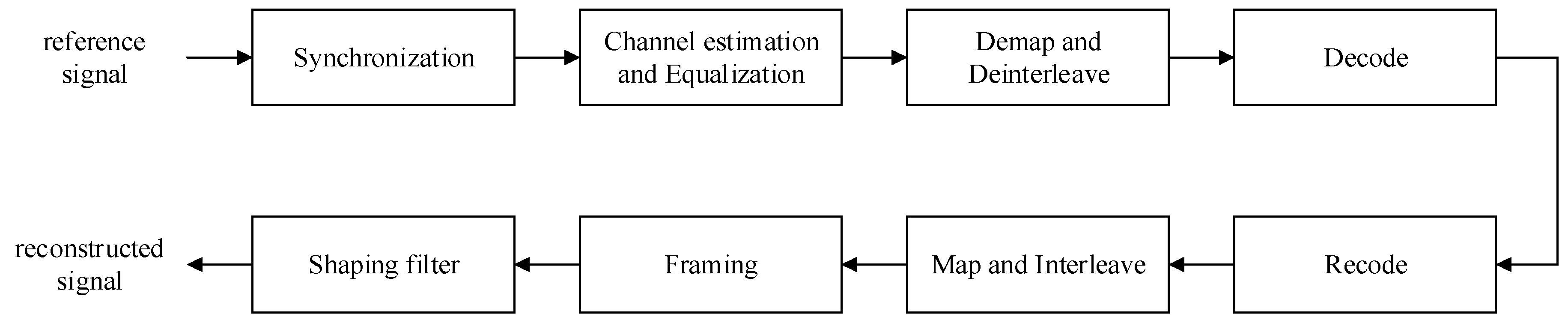
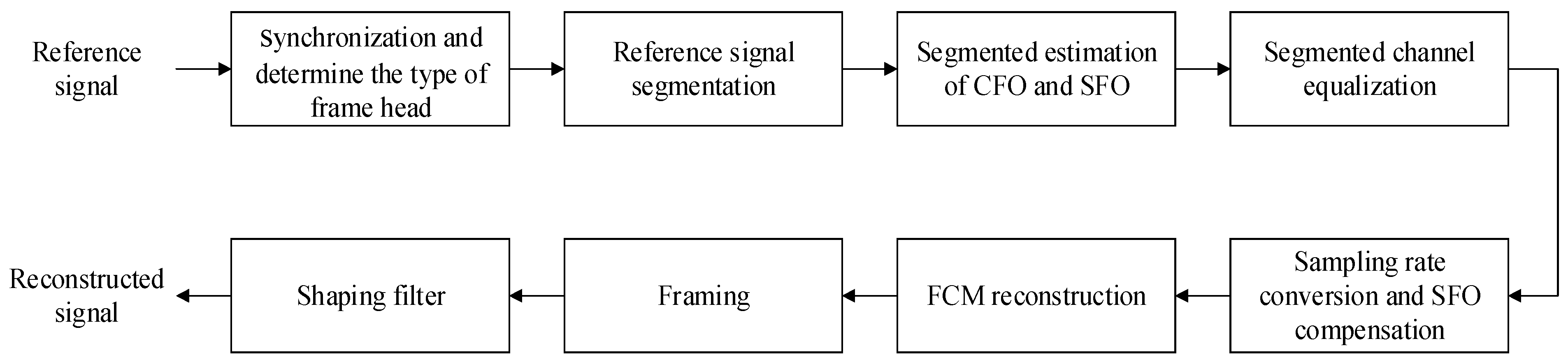
3.1. The Process of Reference Signal Reconstruction

The structure of DTMB signals has the ability to resist multipath interference and noise. Under specific SNR conditions, interference in the reference signal can be effectively suppressed through signal reconstruction. The signal reconstruction process involves various stages including synchronization, channel estimation and equalization, constellation demapping, and decoding. Subsequently, the signal is remapped and shaped according to the standard protocol to obtain the original baseband transmission signal, thus obtaining a purified reference signal. A comprehensive description of the reconstruction scheme at the reception is shown in Figure 4.

3.1.1. Synchronization

In DTMB systems, the accurate synchronization processing of the received data at the receiver is crucial. Without precise synchronization, divergence and phase rotation may occur in the constellation diagram, which will lead to an increased BER of signal reconstruction. The DTMB signal ingeniously utilizes PN sequences as FH, which have exceptional autocorrelation characteristics to facilitate rapid and accurate synchronization. This method has significant advantages in operation simplicity and excellent performance. In the field of DTMB synchronization technology, synchronization is typically divided into frame, carrier frequency, and sample rate synchronization.

The digital television signal transmitter operates on the basis of signal frames as its fundamental unit. To ensure accurate signal recovery at the receiver, frame synchronization must be realized, which requires the identification of the starting position of the signal frame. Considering the fixed PN sequence in the FH of DTMB signals, the identification of the digital television signal FH type relies on the well-correlated characteristics of the PN sequence [44]. By conducting cross-correlation between the known PN sequence and the signal, the peak position is served as an estimate of the frame header position. The calculation process is given by

$$Xcorr=E\left\{pn•s^{\ast }\right\}$$

(2)

where $pn$ is the known FH, and $s^{*}$ is the complex conjugation of the received signal.

Carrier frequency synchronization is essential for ensuring accurate frequency alignment between the receiver and transmitter, as well as among the individual subcarrier frequencies [45]. For DTMB signals, only considering the OFDM symbol of the FB, the output of the transmitter after inverse Fourier transform can be expressed as

$$s(n)=\frac{1}{\sqrt{N_c}}{\displaystyle \sum _{k=0}^{N_c-1}{S}_k\exp \left(j\frac{2\pi }{N_c}nk\right)n=0,1,\cdots ,N_c-1}$$

(3)

where $N_c$ represents number of subcarriers, and $S_k$ represents the Fourier transform of $s(n)$ with respect to $n$. After the signal $s(n)$ passes through the discrete multipath fading channel $h(n)$ with noise $w(n)$, in the case of ideal synchronization, the received signal $r(n)$ is given by

$$\begin{array}{ll}r(n)& =s(n)\otimes h(n)+w(n)\\ & =\frac{1}{\sqrt{N_c}}{\displaystyle \sum _{k=0}^{N_c-1}{S}_k{H}_k\exp \left(j\frac{2\pi }{N_c}nk\right)}+w(n)\end{array}$$

(4)

where $H_k$ is the Fourier transform of $h(n)$ with respect to $n$. The carrier frequency offset (CFO) originates from the differences in oscillator frequency between the transmitter and receiver, which may arise due to inherent instability in the oscillators or fluctuations of the transmission channel affected by environmental factors [46]. Assuming that the CFO is $\Delta f_c$, the relative CFO is $\epsilon =\Delta f_c/f={\epsilon }_I+{\epsilon }_F$ with $f$ being the symbol rate of OFDM. ${\epsilon }_I$ and ${\epsilon }_F$ are the integer and decimal part of $\epsilon$, respectively. The received signal $r_{\epsilon }(n)$ can be expressed as

$$\begin{array}{ll}{r}_{\epsilon }(n)& =\left[s(n)\otimes h(n)\right]\cdot \exp \left(j\frac{2\pi }{N_c}\epsilon n\right)+w(n)\\ & =\frac{1}{\sqrt{N_c}}{\displaystyle \sum _{k=0}^{N_c-1}{S}_k{H}_k\exp \left(j\frac{2\pi }{N_c}nk\right)\cdot \exp \left(j\frac{2\pi }{N_c}\epsilon n\right)}+w(n).\end{array}$$

(5)

The Fourier transform of $r_{\epsilon }(n)$ with respect to $n$ is

$$R_k=S_{k-{\epsilon }_I}{H}_{k-{\epsilon }_I}\exp \left(j\pi {\epsilon }_F\frac{N_c-1}{N_c}\right)\frac{\sin (\pi {\epsilon }_F)}{N_c\sin (\pi {\epsilon }_F/N_c)}+I_k+W_k$$

(6)

where $W_k$ is the Fourier transform of $w(n)$ with respect to $n$, and $I_k$ is the inter-carrier interference caused by CFO.

$$I_k={\displaystyle \sum _{\begin{array}{c}l=0\\ l\ne k-{\epsilon }_I\end{array}}^{N_c-1}{S}_l{H}_l\exp \left(j\pi {\epsilon }_F\frac{N_c-1}{N_c}\right)\exp \left(-j\pi \frac{l-k+{\epsilon }_I}{N_c}\right)\frac{\sin (\pi {\epsilon }_F)}{N_c\sin (\pi (l-k+{\epsilon }_I+{\epsilon }_F)/N_c)}}.$$

(7)

When ${\epsilon }_F=0$, Equation (6) can be simplified as

$$R_k=S_{k-{\epsilon }_I}{H}_{k-{\epsilon }_I}+W_k.$$

(8)

Although the integer partial frequency offset will not destroy the orthogonality between subcarriers, it will cause the sampled signal to shift in the frequency domain, resulting in cyclic shift after OFDM demodulation and demodulation errors.

When ${\epsilon }_I=0$, Equations (6) and (7) can be simplified as

$$R_k=S_k{H}_k\exp \left(j\pi {\epsilon }_F\frac{N_c-1}{N_c}\right)\frac{\sin (\pi {\epsilon }_F)}{N_c\sin (\pi {\epsilon }_F/N_c)}+I_k+W_k$$

(9)

$$I_k={\displaystyle \sum _{\begin{array}{l}l=0\\ l\ne k\end{array}}^{N_c-1}{S}_l{H}_l\exp \left(j\pi {\epsilon }_F\frac{N_c-1}{N_c}\right)\exp \left(-j\pi \frac{l-k}{N_c}\right)\frac{\sin (\pi {\epsilon }_F)}{N_c\sin (\pi (l-k+{\epsilon }_F)/N_c)}}$$

(10)

where the term $\sin (\pi {\epsilon }_F)/(N_c\sin (\pi {\epsilon }_F/N_c))$ caused by ${\epsilon }_F$ is an amplitude attenuate function on each subcarrier, and the phase is rotated by $\pi {\epsilon }_F(N_c-1)/N_c$ on each subcarrier. Therefore, CFO will increase the BER of the reconstructed signal. According to the structure of digital television signal frames, CFO can be estimated by using the phase difference of the PN sequence in adjacent frames on the basis of frame synchronization. The Fast Fourier Transform (FFT) algorithm also serves as a valuable tool for obtaining a rough estimate of the CFO. The estimation accuracy of this method is improved by increasing the number of FFT points $N$. After the FFT, the synchronization header signal exhibits a characteristic spectrum characterized by obvious peaks. A reliable estimate of the CFO is provided by the displacement of the peak relative to the zero frequency.

Due to the inevitable defects in synchronization and clock stability between transmitter and receiver, there exists a difference between the actual sampling rate and the nominal sampling rate at the receiver [47], known as sampling frequency offset (SFO). The transmitted signal can be approximated as

$$s(t)=\frac{1}{\sqrt{N_c}}{\displaystyle \sum _{k=0}^{N_c-1}{S}_k\exp \left(j2\pi \left(\frac{k}{N_c}\right)\left(\frac{t}{T_s}\right)\right)}$$

(11)

where $T_s$ is the sample interval, $f_s=1/T_s$ is the nominal sampling rate at the transmitter, and the sampling rate at the receiver is $f_s^{\prime }=f_s+\Delta f_s,T_s^{\prime }=1/f_s^{\prime }=T_s+\Delta T_s$. Affected by SFO only, the $g$-th sampling value in the $d$-th frame of the received DTMB signal can be expressed as

$$\begin{array}{ll}e(g)& =s(t){|}_{t=g{T}_s^{\prime }+(d{N}_d+N_h)\ast \Delta T_s}\\ & =\frac{1}{\sqrt{N_c}}{\displaystyle \sum _{k=0}^{N_c-1}{S}_k\exp \left(j2\pi \left(\frac{k}{N_c}\right)\left(\frac{g{T}_s^{\prime }}{T_s}+\frac{(d{N}_d+N_h)\ast \Delta T_s}{T_s}\right)\right)}\end{array}$$

(12)

where $N_d$ is the number of symbols in a frame and $N_h$ is the number of symbols in an FH. The OFDM modulation for the sampled data of the $d$-th frame is as follows

$$\begin{array}{ll}{E}_k& ={\displaystyle \sum _{m=0}^{N_c-1}\frac{1}{\sqrt{N_c}}{\displaystyle \sum _{k=0}^{N_c-1}{S}_k\exp \left(j2\pi \left(\frac{k}{N_c}\right)\left(\frac{n{T}_s^{\prime }}{T_s}+\frac{(d{N}_d+N_h)\ast \Delta T_s}{T_s}\right)\right)\exp \left(-\frac{j2\pi nm}{N_c}\right)}}\\ & =\frac{1}{\sqrt{N_c}}{\displaystyle \sum _{k=0}^{C-1}{S}_k\frac{\sin \left[\pi (\frac{k{T}_s^{\prime }}{T_s}-m)\right]}{\sin \left[\frac{\pi (\frac{k{T}_s^{\prime }}{T_s}-m)}{N_c}\right]}}\exp \left(j2\pi \left(\frac{k}{N_c}\right)\left(\frac{(d{N}_d+N_h)\ast \Delta T_s}{T_s}\right)\right)\exp \left(j\pi (\frac{k{T}_s^{\prime }}{T_s}-m)(1-\frac{1}{N_c})\right).\end{array}$$

(13)

According to Equation (13), the SFO will cause the shift in the FFT period, destroy the orthogonality between subcarriers, and lead to inter-carrier interference (ICI). Cumulative clock offset may result in time drift and potential Inter-Symbol Interference (ISI), accompanied by the phase rotation of each subcarrier. These effects are shown as divergence in the constellation diagram of the signal and an increase in the BER of the reconstructed signal. It may affect the performance of interference cancellation, thereby resulting in Doppler sidelobe energy leakage. SFO influences both the time and frequency domains. Consequently, SFO can be estimated in the time domain by using the autocorrelation characteristics of $\delta$-like functions of the DTMB signal’s PN sequence.

3.1.2. Channel Estimation and Equalization

The reference signal of digital television is affected by both noise interference in the transmission channel and multipath interference caused by reflections from ground, buildings, and other objects. In order to accurately reconstruct the transmitted signal at the receiver, it is imperative to not only achieve synchronization but also estimate the transmission channel and equalize the reference signal [48].

In the digital television signal transmission system, the original transmitted signal matrix $S$ can be expressed as

$$S=\left[\begin{array}{cccc}s(0)& s(1)& \cdots & s(n-1)\\ s(1)& s(2)& & s(n)\\ ⋮& & \ddots & ⋮\\ s(n-1)& s(n)& \cdots & s(2n-2)\end{array}\right].$$

(14)

The reference signal received can be expressed as

$$r=Sd+m$$

(15)

where the channel response vector is $d={\left[d(0),d(1),\cdots ,d(n-1)\right]}^T$, the noise vector is $m={\left[m(0),m(1),\cdots ,m(n-1)\right]}^T$, and received signal vector is $r={\left[r(0),r(1),\cdots ,r(n-1)\right]}^T$.

The estimated channel can be expressed as

$$r=S\stackrel{\wedge }{d}.$$

(16)

The square of the difference between the estimated channel and actual channel is minimized to make the estimated channel close to reality. The objective function $J(\stackrel{\wedge }{d})$ can be expressed as

$$\begin{array}{ll}J(\stackrel{\wedge }{d})& ={‖r-S\stackrel{\wedge }{d}‖}^2\\ & =(r-S\stackrel{\wedge }{d}{)}^{\mathrm{H}}(r-S\stackrel{\wedge }{d})\\ & =r^{\mathrm{H}}r-r^{\mathrm{H}}S\stackrel{\wedge }{d}-\stackrel{\wedge }{d^{\mathrm{H}}}{S}^{\mathrm{H}}r+\stackrel{\wedge }{d^{\mathrm{H}}}{S}^{\mathrm{H}}S\stackrel{\wedge }{d}\end{array}$$

(17)

where the superscript $\mathrm{H}$ represents the conjugate transpose. In order to minimize the sum of squared error, taking the first-order partial derivative of the above objective function with respect to $\stackrel{\wedge }{d}$ gives

$$\frac{\partial (J(\stackrel{\wedge }{d}))}{\partial (\stackrel{\wedge }{d})}=-2r^{\mathrm{H}}S+2\stackrel{\wedge }{d^{\mathrm{H}}}{S}^{\mathrm{H}}S.$$

(18)

The best estimate of the transmission channel is

$$\stackrel{\wedge }{d}={(S^{\mathrm{H}}S)}^{-1}{S}^{\mathrm{H}}r.$$

(19)

After estimating the transmission channel, equalization methods are typically used to suppress multipath interference. Figure 5 shows the principle diagram of equalization, where $S$ represents the transmitted signal matrix, $r$ represents the received signal passing through the channel with response $d$ and polluted by additive noise, and $S^{\prime }$ represents the equalized signal matrix.

The system function $d^{\prime }(z)$ of the equalization filter and the channel transfer function $d(z)$ satisfy

$$d^{\prime }(z)d(z)=1.$$

(20)

Based on the estimated channel response, the system function of the channel equalization filter can be obtained.

3.1.3. Decoding

After the equalization and deinterleaving, there still exist a lot of bit errors. DTMB’s coding and decoding mechanism can decrease the errors more. The DTMB standard suggests the use of Bose–Chaudhuri–Hocquenghem (BCH) combined with LDPC coding as the Forward Error Correction (FEC) design. The decoding of LDPC codes uses the minimum sum algorithm of belief propagation (BP). The core idea of the algorithm is to use the received soft information to iterate between the variable node and the check node.

Then, the decoded data stream is mapped, interleaved, and framed with the FH. The signal is converted to the actual sampling rate to obtain the reconstructed signal. For DTMB signals, the received reference signal frame time is as long as seconds [49]. The increased divergence and phase rotation are caused by the accumulation of CFO and SFO estimation errors. In the meantime, the computational cost is increased by error correction decoding. This poses significant challenges for engineering applications and real-time processing. Therefore, there is an urgent need to optimize the reconstruction process, aiming to minimize computational cost and facilitate application in engineering scenarios.

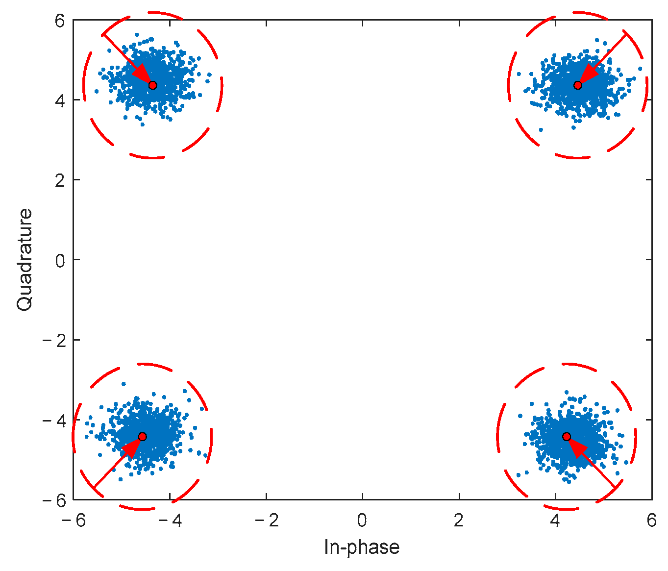
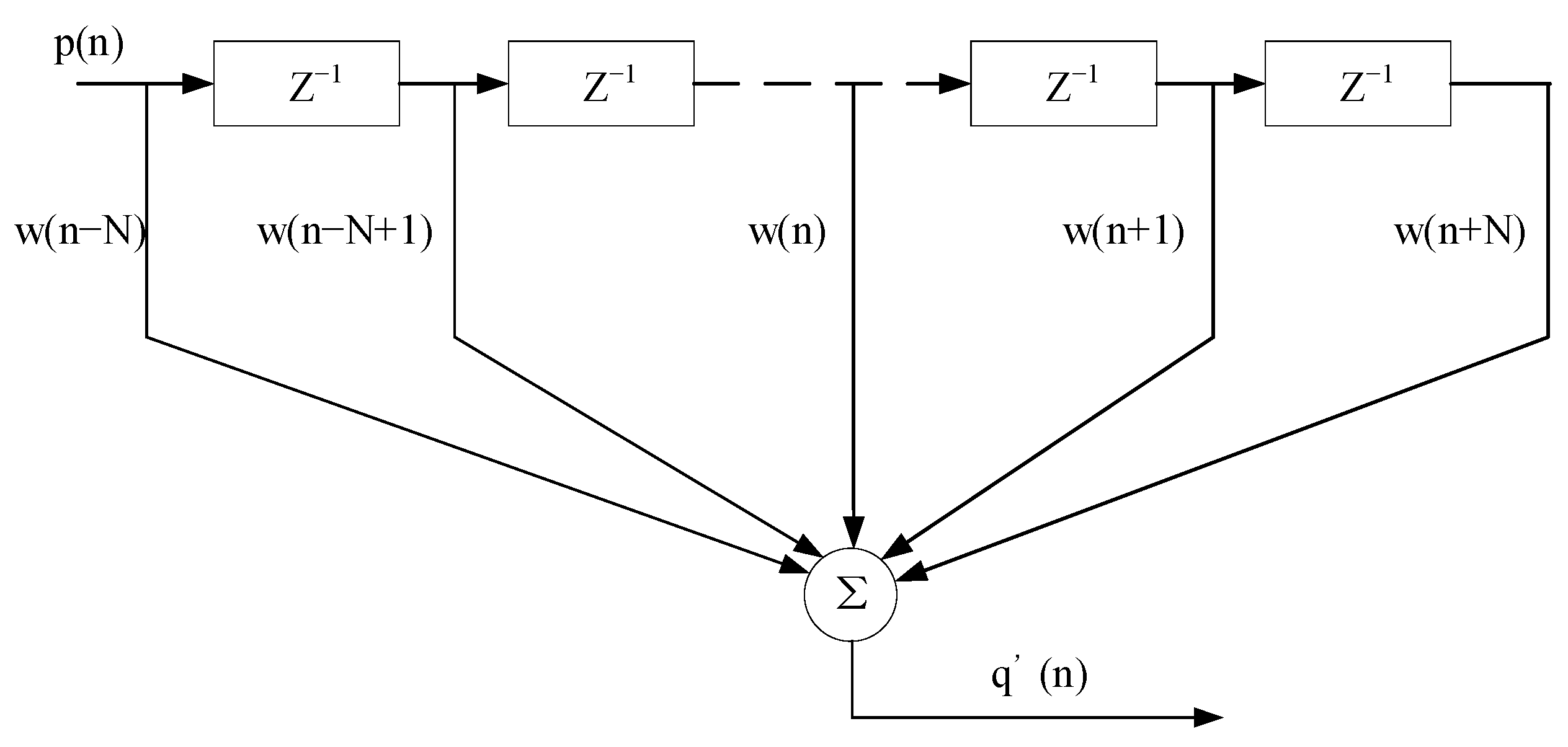
3.2. Segmented Sliding Window Reference Signal Reconstruction Method Based on Fuzzy C-Means

In order to satisfy the system’s real-time processing demands and minimize computational resource consumption, this article proposes a segmented sliding window reconstruction method based on FCM.

The traditional method and the block structure designed for DTMB signals in this article are shown in Figure 6. The received reference signal is taken as one data block for frequency offset and sampling rate deviation estimation in the traditional method. In contrast, the approach proposed effectively works by dividing the signal into different data blocks based on the number of frames, which reduces the accuracy requirement of deviation estimation. In each block, frequency offset and sampling rate deviation are estimated independently, and the data block is compensated based on the estimated values. Notably, there is an overlap of signal frames between different data blocks, which ensures the continuity of the reconstructed signal. Furthermore, FCM clustering is used to map the data to cluster centers instead of LDPC decoding. According to the data membership to the cluster centers, the data are remapped to the center values to complete the reconstruction process.

Figure 7 shows the 4QAM signal frame constellation. The presence of distinct clustering centers in the constellation diagram is readily apparent. The data can be classified into respective cluster centers by utilizing clustering methods. FCM clustering determines the probability of data belonging to a specific class by the size of membership [50,51]. This method is suitable for all types of PN headers in DTMB, thus improving the effectiveness of the reconstruction process.

The process of the segmented sliding window reconstruction method based on FCM is shown in Figure 8.

Step1: Based on the structural properties of digital television signal frames, autocorrelation analysis is conducted in the reference signal. By combining the relationship between the baseband data sampling rate and 7.56 MHz, the frame length of three distinct PN headers is converted to the frame length under the baseband data sampling rate, which is expressed as

$$L=\frac{f_s}{7.56\times {10}^6}\times L_{PN}PN=420,595,945$$

(21)

where $f_s$ is actual baseband data sampling rate, and $L_{PN}$ is the frame length of different types of digital television signal frames at 7.56 MHz. Comparing the peak positions of the signal autocorrelation results and frame length, the frame header pattern and data type of the reference signal can be determined. In the case of PN595 and PN420 with a zero phase, along with PN945, the peak position identified in the cross-correlation is denoted as the precise location of the FH signal. However, for PN headers of the cyclic shift variety, the additional synchronization of the frame header sequence number becomes essential after the determination of the estimated frame header position.

In the example of PN420 in cyclic shift mode, the 225 PN420 sequences exhibit a symmetrical distribution centered around the 112th sequence. Notably, the maximum difference occurs within the interval spanning the 111th and 112th sequences, whereas the minimum difference is observed between the 112th and 113th sequences. The difference between the frame header positions is utilized to estimate frame header position, which is derived from the primary PN sequence correlation. By identifying the positions with the maximum and minimum differences, the frame header sequence position can be obtained.

According to the FH position and data type corresponding to the reference signal, each segment of the reference signal is denoted as $x(n)$, and each segment of the echo signal is denoted as $y(n)$, with $N_k$ segments in total. The frame number of each signal segment $N_m$ is shown in Equation (22), and the step number of each signal segment $N_s$ is shown in Equation (23).

$$N_m=N_{PN}/N_k+1PN=420,595,945$$

(22)

$$N_s=N_{PN}/N_{k}PN=420,595,945.$$

(23)

where $N_{PN}$ is the number of signal frames of different types of signals in the acquisition time at the 7.56 MHz.

Step2: The process of N-point FFT on the reference signal $x(n)$ is given by

$$X(k)={\displaystyle \sum _{n=0}^{N-1}x(n)e^{-j\frac{2\pi nk}{N}}}$$

(24)

where $X(k)$ represents the FFT results of the reference signal. According to the position corresponding to the peak of spectral line, the frequency offset value can be expressed as

$$\left|X(k_{\mathrm{f}})\right|=\underset{k}{\max }\left|X(k)\right|0\le k\le L-1.$$

(25)

The CFO is given by

$$CFO=k_f/(f_{s}N).$$

(26)

To compensate frequency offset, the reference signal $x_c(n)$ and the echo signal $y_c(n)$ are given by

$$x_c(n)=x(n)\cdot \exp \left(-j2\pi \cdot CFO\cdot n{f}_s\right)$$

(27)

$$y_c(n)=y(n)\cdot \exp \left(-j2\pi \cdot CFO\cdot n{f}_s\right)$$

(28)

where $n=\left[1,2,3,\cdots ,i\right]$, and $i$ denotes the number of data points in this segment.

Based on the symbol rate $B_s$ of the transmitting station, $f_s$ represents the nominal value of the sampling frequency, $f_s^{\prime }$ represents the actual value, and the theoretical position of the $k$-th correlation peak corresponding to the $k$-th frame can be expressed as

$$p{n}_n=round(k{N}_{symbol}{f}_s/B_s)$$

(29)

where $N_{symbol}$ indicates the number of symbols in one signal frame, and the actual position of the correlation peak corresponding to the $k$-th frame can be expressed as

$$p{n}_n^{\prime }=round(k{N}_{symbol}{f}_s^{\prime }/B_s).$$

(30)

The SFO is given by

$$SFO=\frac{(p{n}_n^{\prime }-p{n}_n)B_s}{k{N}_{symbol}}.$$

(31)

Step3: The transverse filter, commonly employed for equalization, is widely utilized in practical applications. However, due to the limitations in the filter order, it cannot completely eliminate multipath interference, but it can maximize interference suppression. Figure 9 shows the structure of the 2N + 1 order transversal filter.

The Minimum Mean Square Error (MMSE) equalization criterion is used in this article. MMSE equalization adjusts the coefficients of the transversal filter to minimize the mean square error of the output signal. Since the digital television signal frame type can be determined at the receiver end, the equalization filter coefficients can be solved using the standard PN sequence and the received PN sequence.

The coefficient of 2N + 1 order filter is $w_n={\left[w(n-N),\cdots ,w(n),\cdots w(n+N)\right]}^T$, the vector of the received PN sequence is $p_n={\left[p(n-N),\cdots ,p(n),\cdots ,p(n+N)\right]}^T$, and the output signal of the equalization filter can be expressed as

$$q^{\prime }(n)=w_n^{\mathrm{H}}{p}_n.$$

(32)

The mean square error is

$$\begin{array}{ll}J(w)& =E\left[{\left|q(n)-w_n^{\mathrm{H}}{p}_n\right|}^2\right]\\ & =E\left[{\left|q(n)\right|}^2\right]-2re\left\{w_n^{\mathrm{H}}E\left[q^{*}(n)p_n\right]\right\}+w_n^{\mathrm{H}}E\left[p_n{p}_n^{\mathrm{H}}\right]w_n\end{array}$$

(33)

where $q(n)$ represents the $n$-th symbol of a standard PN sequence, $q^{*}(n)$ represents the conjugation of $q(n)$, and $re\left\{\cdot \right\}$ represents the real part of the complex. For stationary signals, the autocorrelation matrix is non-negative, and the mean square error is a quadratic function and only has one minimum value.

Then, the MMSE equalization filter coefficient is given by

$$w_{opt}=R_{xx}^{-1}{r}_{xs}$$

(34)

where $R_{xx}=E\left[p_n{p}_n^{\mathrm{H}}\right]$ represents the autocorrelation matrix of the PN sequence, and $r_{xs}=E\left[q^{*}(n)p_n\right]$ represents the cross-correlation vector of PN sequence. Each reference signal is filtered by the equalization filter coefficient, and the equalization process in the frequency domain is expressed as

$$x_e(k)=w_k\odot x(k)$$

(35)

where $x_e(k)$ is the frequency domain expression of $x_e(n)$, $x(k)$ is the frequency domain expression of $x(n)$, and $w_k$ is the frequency domain expression of $w_{opt}$. $\odot$ is Hadamard product, which represents corresponding position elements’ multiplication of the vector.

Step4: The $x_e(n)$ is resampled to the common multiple of the baseband sampling rate and 7.56 MHz, and it is filtered by using a square root raised cosine (SSRC) filter with a roll-off coefficient of 0.05. The filter frequency response is as follows:

$$H_s(f)=\left\{\begin{array}{cc}1& \begin{array}{c},\left|f\right|>f_N(1-\alpha )\end{array}\\ {\left\{\frac{1}{2}+\frac{1}{2}\cos \frac{\pi }{2f_N}(\frac{\left|f\right|-f_N(1-\alpha )}{\alpha })\right\}}^{\frac{1}{2}}& ,f_N(1-\alpha )<\left|f\right|<f_N(1+\alpha )\\ 0& \begin{array}{c},\left|f\right|>f_N(1+\alpha )\end{array}\end{array}\right.$$

(36)

where $f_N$ is the Nyquist frequency. The data from each segment are sampled down to the baud rate of 7.56 MHz. Meanwhile, SFO is compensated in the down-sampling process.

Then, the FCM method is utilized for data clustering, which obtains cluster centers by minimizing an objective function. The sum of Euclidean distances from each point to each cluster center is essentially represented with this objective function. The clustering process is involved in minimizing this objective function through iterative computations, gradually reducing the error value. Upon convergence of the objective function, the final clustering results are obtained.

The Euclidean distance from each data point to the cluster center can be expressed as

$$D={\displaystyle \sum _{k=1}^L{\displaystyle \sum _{i=1}^N{u}_{ki}{‖b_i-c_k‖}^2,}}s.t{\displaystyle \sum _{k=1}^L{u}_{ki}=1,i=1,2,\cdots ,N}$$

(37)

where $b_i$ represents the $i$-th data point, $c_k$ represents the $k$-th cluster center, and $u_{ki}$ represents the probability that point $i$ belongs to the $k$ cluster. Set the number of clusters $k$ and threshold $\epsilon$, initialize membership matrix $u$, and calculate clustering center of each cluster as

$$c_k=\frac{{\displaystyle \sum _{i=1}^N{u}_{ki}{b}_i}}{{\displaystyle \sum _{i=1}^N{u}_{ki}}}.$$

(38)

The LaGrange multiplier is constructed for optimizing the cluster center, as shown in Equation (39). When $L\ge \epsilon$, Equation (40) is used to update the membership matrix until the cluster centers are obtained:

$$L(u_{ki},c_k)={\displaystyle \sum _{k=1}^L{\displaystyle \sum _{i=1}^N{u}_{ki}{‖b_i-c_k‖}^2-{\displaystyle \sum _{i=1}^N{\lambda }_i({\displaystyle \sum _{k=1}^L{u}_{ki}-1)}}}}$$

(39)

$$u_{ki}=\frac{\frac{1}{{‖b_i-c_k‖}^2}}{{\displaystyle \sum _{k=1}^L\frac{1}{{‖b_i-c_k‖}^2}}}.$$

(40)

4. Simulation and Experimental Verification

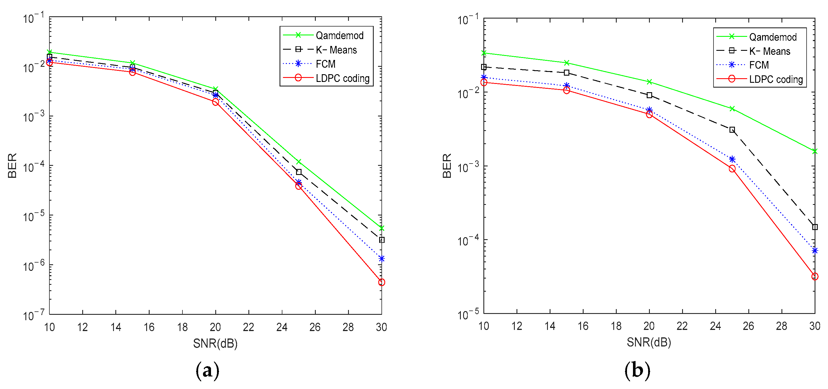
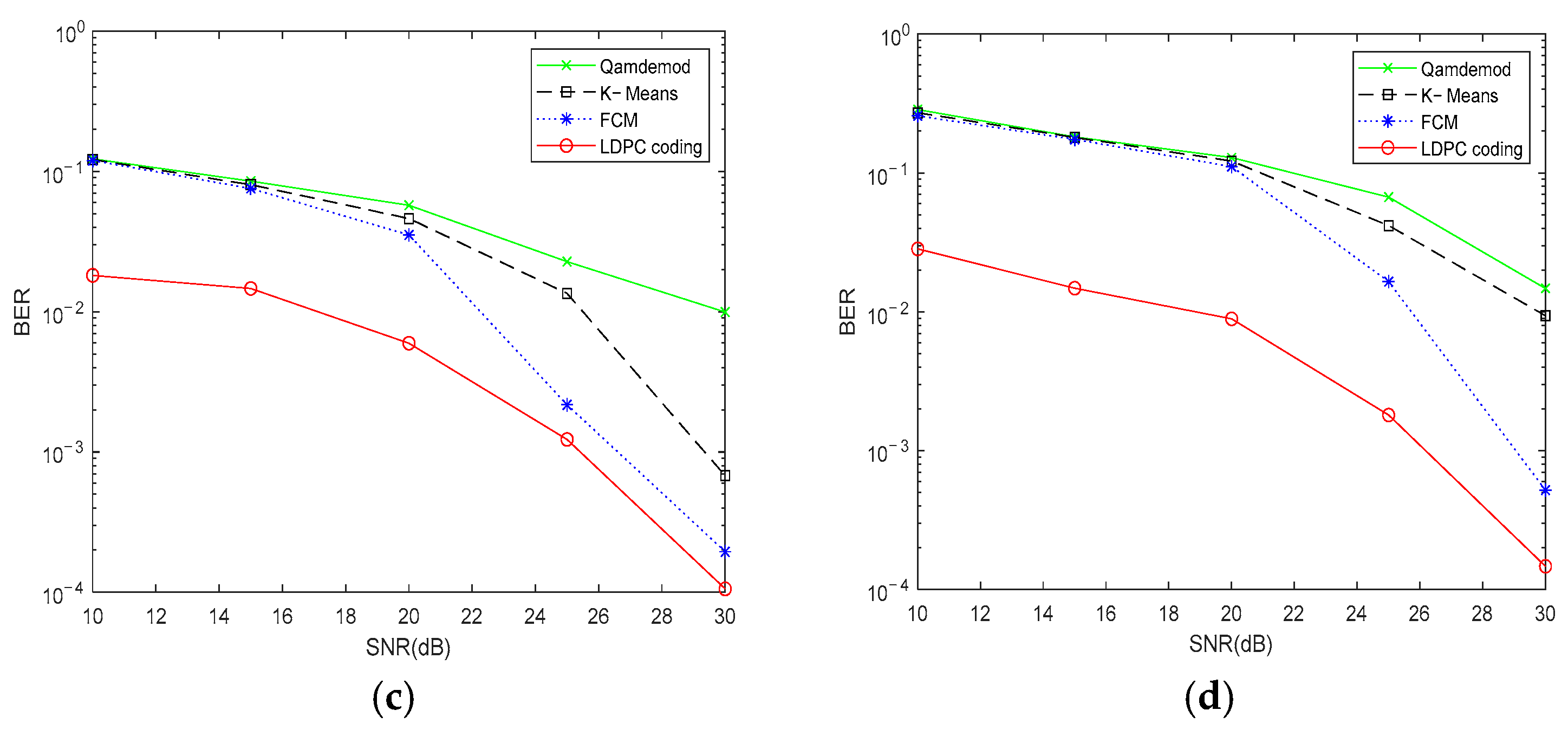
4.1. Simulation Analysis

In order to evaluate the effect of the proposed method in this article on the BER under the conditions characterized by different SNRs, multi-carrier PN420 signals with identical bit rates and four distinct mapping modes are generated through simulation. Four distinct signals are subjected to Gaussian white noise interference at different SNRs. The interfered data are synchronized, equalized, and then converted to the baud rate of 7.56 MHz.

The data are reconstructed utilizing four different methods, including LDPC error correction decoding, K−Means, FCM clustering, and MATLAB’s QAM modulation function ‘Qamdemod’. We initialized the number of clusters as $k=4,16,32,64$, the threshold of Fuzzy C-Means as $\epsilon =0.001$, and the membership matrix as $u=0$. The results are shown in Figure 10.

It is evident that the BER of the proposed method and LDPC decoding are similar for the 4QAM and 16QAM modulation methods. The BER of K−Means and Qamdemod are slightly higher than the preceding two methods. For the 32QAM and 64QAM modulation methods, the BER of FCM clustering is higher than LDPC decoding in low SNR scenarios, but it is close to LDPC decoding under high SNR conditions. The BER change trend of the K−Means method is similar to that of FCM, but it has higher BER. The Qamdemod method exhibits a significantly higher BER.

This observation can be attributed to the fact that simpler constellation mapping has fewer cluster centers and is more easily clustered. In addition, the high SNR constellation is more clustered, which makes it easier to identify the clustering center of each data point. In contrast, in the 32QAM and 64QAM mapping modes, it is difficult to accurately determine cluster centers under low-SNR conditions due to constellation diagram divergence.

Then, for the same data, we compared the running time of FCM clustering and LDPC decoding under the same computer configuration, as shown in

Table 1. Algorithm running time.

Symbol Constellation Mapping Mode	Symbol Reconstruction Algorithm	Running Time (s)
4QAM	LDPC decoding	5.0938
	FCM	0.3512
16QAM	LDPC decoding	176.0781
	FCM	12.7384
32QAM	LDPC decoding	247.6813
	FCM	17.6915
64QAM	LDPC decoding	365.4063
	FCM	25.6605

. It can be seen that the operation time consumption of the FCM clustering method is much less than LDPC decoding.

The reason is that LDPC decoding involves multiplication with the check matrix, and it needs to be iterated until the result converges to zero. The check matrix properties of LDPC codes are shown in

Table 2. The check matrix properties of LDPC codes.

Coding Rate	Line Number (M)	Column Number (N)	Sum of Row Weight (L)
0.4	4445	7493	34,925
0.6	2921	7493	37,592
0.8	1397	7493	37,338

. $L$ represents the number of one in the row, $M$ is the line number of the check matrix, and $N$ is the column number of the check matrix. In the process of LDPC decoding using the check matrix, the number of matrix operations involved in one frame is shown in

Table 3. The number of matrix operations with different coding rates in LDPC decoding.

Coding Rate	Addition	Multiplication	Comparison
0.4	77,343	62,357	37,973
0.6	82,677	67,681	42,164
0.8	82,169	67,138	43,434

. The calculation of the addition operation is represented as $2L+N$, the multiplication operation is represented as $2L-N$, and the comparison operation is represented as $L+N-M$. These matrix operations may lead to a large computation cost. However, the number of matrix operations with different coding rates in FCM is only affected by mapping modes. It can be represented as $k_{\mathrm{mod}e}·n$, where $k_{\mathrm{mod}e}$ is the number of clustering centers and $n$ is number of iterations. The results show that the FCM clustering method proposed in this paper has great practicability in symbol mapping reconstruction.

The segmented sliding window reconstruction method based on FCM proposed in this article involves signal segmentation operation. Different lengths of the segmented sliding block affect the performance of the reconstruction method. To analyze the impact of different block lengths on the performance, one second 16QAM multi-carrier PN420 signal is simulated. The different lengths of the block are selected as 45, 90, 135, 180, 225, 450, 675, 900, 1125, 1350, 1575, and 1800 frames. The impact of block length on the performance of the reconstruction method was analyzed by comparing the cancellation gain of the reconstructed signals obtained using different block lengths. The results are shown in Figure 11.

When the block length becomes shorter, the Normalized Least Mean Square (NLMS) cancellation gain increases. However, the estimation time of CFO and SFO is increased. When the block length becomes longer, the time required for one data block sampling rate conversion is increased. The comparation of the calculation time between the traditional method and the proposed method with a block length equal to 225 frames is shown in

Table 4. Calculation times for different reconstruction methods.

Symbol Constellation Mapping Mode	Symbol Reconstruction Algorithm	Running Time (s)
4QAM	Traditional method	103.4792
	Proposed method	89.6374
16QAM	Traditional method	273.4981
	Proposed method	104.1637
32QAM	Traditional method	347.6967
	Proposed method	116.8731
64QAM	Traditional method	469.1237
	Proposed method	143.7413

.

4.2. Experimental Verification

Our laboratory conducted experimental research on LSS target detection with passive radar based on DTMB in Pinggu, Beijing, in 2023.

During the experimental phase, data were collected from both the reference and the surveillance channels. A one-second segment of received data was selected, known to contain a weak target. Subsequently, two separate datasets were prepared for further analysis: the reference signal using the traditional unpartitioned reconstruction method and using the segmented sliding window reference signal reconstruction method based on FCM proposed in this article. The direct waves and clutter in the surveillance channel were suppressed by clutter cancellation for the two datasets. Cross ambiguity functions were conducted for both datasets, with the result used to obtain Range-Doppler results for the purpose of validating the effectiveness and practicality of the method.

The first set of data used the CCTV Tower in Haidian District, Beijing, as the illuminators. The frame header mode was cyclic-shift PN420, the center frequency was 666 MHz, and the system sampling rate was 10 MHz.

The one-second reference signal was divided into eight segments, and each segment was compensated by frequency offset and sampling rate deviation individually and reconstructed by the FCM clustering method. The 900-th frame constellations are shown in Figure 12. The constellation diagram using the traditional unpartitioned method rotates and diverges.

In response to the reconstructed signals obtained from both methods, NLMS cancellation is adopted to suppress direct waves, multipath interference, and noise in the surveillance channel. Compared to the traditional method, the approach proposed in this article has an increased cancellation gain, as shown by the values presented in Figure 13.

Figure 14 shows the results of two different reconstruction methods after adaptive cancellation and cross-ambiguity function. The segmented sliding window reconstruction method based on FCM leads to an enhancement in the detected target amplitude and increases the target SNR from 30.32 dB to 35.76 dB.

The second set of data is a real digital TV signal of Pinggu TV Tower which is located in Pinggu District, Beijing. The received signal contains a weak target. The frame header mode is PN595, the center frequency is 674 MHz, and the system sampling rate is 10 MHz.

The 864-th frame constellations are shown in Figure 15. The constellation diagram using the traditional unpartitioned method rotates and diverges.

NLMS cancellation is adopted to suppress direct and multipath interferences in the surveillance channel. Compared to traditional methods, the approach proposed has an increased cancellation gain, as shown in Figure 16.

Figure 17 shows the results of two different reconstruction methods after adaptive cancellation and the cross-ambiguity function. The segmented sliding window reconstruction method based on FCM leads to an enhancement in the detected target amplitude and increases the target SNR from 19.41 dB to 27.89 dB.

5. Conclusions

In this article, a segmented sliding window reference signal reconstruction method based on FCM was proposed for target detection in passive radar. The frequency offset and sampling rate deviation were estimated for each signal segment, which reduced the accuracy requirement of deviation estimation. This method has effectively suppressed the issues of constellation diagram divergence and phase rotation which arose from error accumulation. The utilization of FCM clustering instead of LDPC error correction decoding for symbol mapping reconstruction contributed to reducing the computation cost. This approach has increased the adaptive cancellation gain and target SNR, which is advantageous for the detection of LSS targets, thus having significant implications for practical engineering applications.

References

1. Huang, X.; Wang, Z.; Peng, Q.; Xu, H.; He, Z. LSS UAV Target Intelligent Detection in Urban Complex Environment. In Proceedings of the 2021 IEEE 3rd International Conference on Civil Aviation Safety and Information Technology (ICCASIT), Changsha, China, 20–22 October 2021; IEEE: New York, NY, USA, 2021; pp. 648–650. [Google Scholar]
2. Fang, M.; Li, L.; Zhao, C.; Guo, Y.; Qi, Z. A LSS-Target Detection Method for Urban Complex Environment. In Proceedings of the 2021 2nd China International SAR Symposium (CISS), Shanghai, China, 3 November 2021; IEEE: New York, NY, USA, 2021; pp. 1–5. [Google Scholar]
3. Chen, S.; Yin, Y.; Wang, Z.; Gui, F. Low-Altitude Protection Technology of Anti-UAVs Based on Multisource Detection Information Fusion. Int. J. Adv. Robot. Syst. 2020, 17, 1729881420962907. [Google Scholar] [CrossRef]
4. Chen, S.; Dang, Y.; Liu, M.; Wang, H.; Lv, F. Surveillance of Ground and LSS Targets: A Radar-Photoelectric Early Warning System. In Proceedings of the 2023 Cross Strait Radio Science and Wireless Technology Conference (CSRSWTC), Guilin, China, 10 November 2023; IEEE: New York, NY, USA, 2023; pp. 1–3. [Google Scholar]
5. Tan, M. Signal Processing Techniques for LFMCW Radar under Urban Low, Slow, and Small Conditions. In Proceedings of the 2024 4th International Conference on Neural Networks, Information and Communication (NNICE), Guangzhou, China, 19 January 2024; IEEE: New York, NY, USA, 2024; pp. 1171–1175. [Google Scholar]
6. Shoufan, A.; Al-Angari, H.M.; Sheikh, M.F.A.; Damiani, E. Drone Pilot Identification by Classifying Radio-Control Signals. IEEE Trans. Inf. Forensics Secur. 2018, 13, 2439–2447. [Google Scholar] [CrossRef]
7. Sun, H.; Liu, Q.; Wang, J.; Ren, J.; Wu, Y.; Zhao, H.; Li, H. Fusion of Infrared and Visible Images for Remote Detection of Low-Altitude Slow-Speed Small Targets. IEEE J. Sel. Top. Appl. Earth Obs. Remote Sens. 2021, 14, 2971–2983. [Google Scholar] [CrossRef]
8. Pang, D.; Shan, T.; Ma, P.; Li, W.; Liu, S.; Tao, R. A Novel Spatiotemporal Saliency Method for Low-Altitude Slow Small Infrared Target Detection. IEEE Geosci. Remote Sens. Lett. 2022, 19, 1–5. [Google Scholar] [CrossRef]
9. Xu, D.; Zhang, H. Study of Low-Altitude Slow and Small Target Detection on Radar. In Proceedings of 2017 5th International Conference on Machinery, Materials and Computing Technology (ICMMCT 2017), Beijing, China, 25–26 March 2017; Atlantis Press: Paris, France, 2017. [Google Scholar]
10. Yu, Q.; Rao, B.; Luo, P. Detection Performance Analysis of Small Target Under Clutter Based on LFMCW Radar. In Proceedings of the 2018 IEEE 3rd International Conference on Signal and Image Processing (ICSIP), Shenzhen, China, 13–15 July 2018; IEEE: New York, NY, USA, 2018; pp. 121–125. [Google Scholar]
11. He, Z.; Sun, J.; Zhang, W.; An, K.; Wang, C.-X. A Passive Broadband Radar System Design for Low, Slow and Small Target Detection. In Proceedings of the 2022 IEEE/CIC International Conference on Communications in China (ICCC Workshops), Sanshui, China, 11 August 2022; IEEE: New York, NY, USA, 2022; pp. 18–23. [Google Scholar]
12. Kuschel, H.; Cristallini, D.; Olsen, K.E. Tutorial: Passive radar tutorial. IEEE Aerosp. Electron. Syst. Mag. 2019, 34, 2–19. [Google Scholar] [CrossRef]
13. Coleman, C.; Yardley, H. Passive bistatic radar based on target illuminations by digital audio broadcasting. IET Radar Sonar Navig. 2008, 2, 366–375. [Google Scholar] [CrossRef]
14. Tao, R.; Wu, H.; Shan, T. Direct-path suppression by spatial filtering in digital television terrestrial broadcasting-based passive radar. IET Radar Sonar Navig. 2010, 4, 791–805. [Google Scholar] [CrossRef]
15. Dawidowicz, B.; Samczynski, P.; Malanowski, M.; Misiurewicz, J. Detection of moving targets with multichannel airborne passive radar. IEEE Aerosp. Electron. Syst. Mag. 2012, 27, 42–49. [Google Scholar] [CrossRef]
16. Palmer, J. A Signal Processing Scheme for a Multichannel Passive Radar System. In Proceedings of the 2015 IEEE International Conference on Acoustics, Speech and Signal Processing (ICASSP), South Brisbane, QL, Australia, 19–24 April 2015; pp. 5575–5579. [Google Scholar]
17. O’Hagan, D.W.; Setsubi, M.; Paine, S. Signal Reconstruction of DVB-T2 Signals in Passive Radar. In Proceedings of the 2018 IEEE Radar Conference (RadarConf), Oklahoma City, OK, USA, 23–27 April 2018; pp. 1111–1116. [Google Scholar]
18. Daun, M.; Nickel, U.; Koch, W. Tracking in multistatic passive radar systems using DAB/DVB-T illumination. Signal Process. 2012, 92, 1365–1386. [Google Scholar] [CrossRef]
19. Choi, S.; Crouse, D.; Willett, P.; Zhou, S. Multistatic target tracking for passive radar in a DAB/DVB network: Initiation. IEEE Trans. Aerosp. Electron. Syst. 2015, 51, 2460–2469. [Google Scholar] [CrossRef]
20. Miao, Y.; Li, J.; Bao, Y.; Liu, F.; Hu, C. Efficient Multipath Clutter Cancellation for UAV Monitoring Using DAB Satellite-Based PBR. Remote Sens. 2021, 13, 3429. [Google Scholar] [CrossRef]
21. Palmer, J.E.; Harms, H.A.; Searle, S.J.; Davis, L. DVB-T passive radar signal processing. IEEE Trans. Signal Process. 2012, 61, 2116–2126. [Google Scholar] [CrossRef]
22. Klincewicz, K.; Samczy’nski, P. Method of Calculating Desynchronization of DVB-T Transmitters Working in SFN for PCL Applications. Sensors 2020, 20, 5776. [Google Scholar] [CrossRef] [PubMed]
23. Colone, F. DVB-T-Based Passive Forward Scatter Radar: Inherent Limitations and Enabling Solutions. IEEE Trans. Aerosp. Electron. Syst. 2021, 57, 1084–1104. [Google Scholar] [CrossRef]
24. Lü, M.; Yi, J.; Wan, X.; Zhan, W. Co-channel Interference in DTMB-Based Passive Radar. IEEE Trans. Aerosp. Electron. Syst. 2019, 55, 2138–2149. [Google Scholar] [CrossRef]
25. Hu, S.; Yi, J.; Wan, X.; Cheng, F.; Hu, Y.; Hao, C. Illuminator of Opportunity Localization for Digital Broadcast-Based Passive Radar in Moving Platforms. IEEE Trans. Aerosp. Electron. Syst. 2023, 59, 3539–3549. [Google Scholar] [CrossRef]
26. Zhang, C.; Li, J.; Gao, P.; Pan, C.; Li, X.; Qi, W.; Yang, F. SFN Structure and Field Trials Based on Satellite Links for DTMB System. In Proceedings of the 2016 IEEE International Symposium on Broadband Multimedia Systems and Broadcasting (BMSB), Nara, Japan, 1–3 June 2016; pp. 1–5. [Google Scholar]
27. Chen, G.; Tian, B.; Gong, J.; Feng, C.Q. Reconstruction of Passive Radar Reference Signal Based on DTMB. In Proceedings of the 2019 IEEE 2nd International Conference on Information Communication and Signal Processing (ICICSP), Weihai, China, 28–30 September 2019; pp. 170–174. [Google Scholar]
28. Garry, J.L.; Baker, C.J.; Smith, G.E. Evaluation of Direct Signal Suppression for Passive Radar. IEEE Trans. Geosci. Remote Sens. 2017, 55, 3786–3799. [Google Scholar] [CrossRef]
29. Wan, X.; Cheng, Y.; Tang, H.; Liu, Y. The Effects of Non-Ideal Factors on Clutter Cancellation in DTMB-Based Passive Radar. In Proceedings of the 2017 IEEE Radar Conference (RadarConf), Seattle, WA, USA, 8–12 May 2017; pp. 1440–1445. [Google Scholar]
30. Feng, W.; Friedt, J.M.; Cherniak, G.; Sato, M. Batch compressive sensing for passive radar range-Doppler map generation. IEEE Trans. Aerosp. Electron. Syst. 2019, 55, 3090–3102. [Google Scholar] [CrossRef]
31. Fang, L.; Wan, X.; Fang, G.; Cheng, F. Passive detection using orthogonal frequency division multiplex signals of opportunity without multipath clutter cancellation. IET Radar Sonar Navig. 2016, 10, 516–524. [Google Scholar] [CrossRef]
32. Song, L.Q.; Wang, J.; Pan, C.Y.; Fu, J. A Normalized LLR Soft Information Demapping Method in DTMB System. In Proceedings of the 2008 11th IEEE Singapore International Conference on Communication Systems (ICCS), Guangzhou, China, 19–21 November 2008; pp. 1297–1301. [Google Scholar]
33. Wu, Y.; Chen, Z.; Peng, D. Target Detection of Passive Bistatic Radar under the Condition of Impure Reference Signal. Remote Sens. 2023, 15, 3876. [Google Scholar] [CrossRef]
34. Zuo, L.; Wang, J.; Zhao, T.; Cheng, Z. A Joint Low-Rank and Sparse Method for Reference Signal Purification in DTMB-Based Passive Bistatic Radar. Sensors 2021, 21, 3607. [Google Scholar] [CrossRef] [PubMed]
35. Berger, C.R.; Demissie, B.; Heckenbach, J.; Willett, P. Signal Processing for Passive Radar Using OFDM Waveforms. IEEE J. Sel. Top. Signal Process. 2010, 4, 226–238. [Google Scholar] [CrossRef]
36. Tang, H.; Wan, X.; Liu, Y.; Cheng, Y.; Yi, J. On the Performance of Multipath in Reference Signal for Passive Radar Interference Cancellation. In Proceedings of the 2017 IEEE Radar Conference (RadarConf), Seattle, WA, USA, 8–12 May 2017; pp. 1313–1316. [Google Scholar]
37. Xiang, O.Y.; Ruan, C.C.; Zheng, L.X. Implementation of LDPC Encoding to DTMB Standard Based on FPGA. In Proceedings of the 2011 10th IEEE/ACIS International Conference on Computer and Information Science (ACIS), Sanya, China, 16–18 May 2011; pp. 235–238. [Google Scholar]
38. Li, Y.; Zhang, Q. The Study for Parameter Configuration of the Reference Network of Chinese Digital Television. In Proceedings of the 2011 4th International Congress on Image and Signal Processing (CISP), Shanghai, China, 15–17 October 2011; pp. 322–326. [Google Scholar]
39. Wu, J.; Chen, Y.; Zeng, X.; Min, H. Robust Timing and Frequency Synchronization Scheme for DTMB System. IEEE Trans. Consumer Electron. 2007, 53, 1348–1352. [Google Scholar] [CrossRef]
40. Yan, K.; Ding, W.; Zhang, L.; Yin, Y.; Yang, F.; Pan, C. Measurement and Prediction of DTMB Reception Quality in Single Frequency Networks. In Proceedings of the 2011 7th International Wireless Communications and Mobile Computing Conference (WiCom), Istanbul, Turkey, 4–8 July 2011; pp. 936–940. [Google Scholar]
41. El-Hajjar, M.; Hanzo, L. A Survey of Digital Television Broadcast Transmission Techniques. IEEE Commun. Surv. Tutor. 2013, 15, 1924–1949. [Google Scholar] [CrossRef]
42. Bournaka, G.; Ummenhofer, M.; Cristallini, D.; Palmer, J.; Summers, A. Experimental Study for Transmitter Imperfections in DVB-T Based Passive Radar. IEEE Trans. Aerosp. Electron. Syst. 2018, 54, 1341–1354. [Google Scholar] [CrossRef]
43. Jin, H.P.; Peng, K.W.; Song, J. Backward Compatible Multiservice Transmission Over the DTMB System. IEEE Trans. Broadcast. 2014, 60, 499–510. [Google Scholar]
44. Bae, J.; Kim, Y.; Hur, N.; Choi, D.-J.; Kim, H.J.; Kim, H.-N. Data Rate Increasing Method Using Multiple PN Sequences for the Superposed PNs on Broadcasting System Signals. In Proceedings of the 2020 IEEE International Conference on Consumer Electronics—Asia (ICCE-Asia), Seoul, Republic of Korea, 1 November 2020; pp. 1–5. [Google Scholar]
45. Zhang, S.; Zhang, X.L.; Zhang, C. A Cyclostationary Frequency Offset Estimation for DTMB System. In Proceedings of the 2008 9th International Conference on Signal Processing (ICSP), Beijing, China, 26–29 October 2008; pp. 1822–1825. [Google Scholar]
46. Sato, A.; Shitomi, T.; Takeuchi, T.; Okano, M.; Tsuchida, K. Transmission Performance Evaluation of LDPC Coded OFDM over Actual Propagation Channels in Urban Area. Examination for next-Generation ISDB-T. In Proceedings of the 2017 IEEE International Symposium on Broadband Multimedia Systems and Broadcasting (BMSB), Cagliari, Italy, 7–9 June 2017; pp. 1–5. [Google Scholar]
47. He, S.; Feng, Y.; Shan, T. A Novel Interference Suppression Method for DTMB-Based Passive Radar. In Proceedings of the 2021 CIE International Conference on Radar (Radar), Haikou, China, 15 December 2021; pp. 2799–2803. [Google Scholar]
48. Blasone, G.P.; Colone, F.; Lombardo, P.; Wojaczek, P. Passive Radar DPCA Schemes with Adaptive Channel Calibration. IEEE Trans. Aerosp. Electron. Syst. 2020, 56, 4014–4034. [Google Scholar] [CrossRef]
49. Wan, X.R.; Wang, J.F.; Hong, S.; Tang, H. Reconstruction of Reference Signal for DTMB-Based Passive Radar Systems. In Proceedings of the 2011 IEEE CIE International Conference on Radar (Radar), Chengdu, China, 24–27 October 2011; pp. 165–168. [Google Scholar]
50. Gao, T.; Li, A.; Meng, F. Research on Data Stream Clustering Based on FCM Algorithm 1. Procedia Comput. Sci. 2017, 122, 595–602. [Google Scholar] [CrossRef]
51. Hou, Z.; Li, C.; Luo, Y.; Li, Q.; Xue, J. Colour Selection for Mosaic Tiles Based on FCM Clustering Algorithm. In Proceedings of the 2022 5th World Conference on Mechanical Engineering and Intelligent Manufacturing (WCMEIM), Ma’anshan, China, 18 November 2022; pp. 1032–1035. [Google Scholar]
Figure 1. Frame structure of DTMB signal.
Remotesensing 16 01813 g001
Figure 2. PN420 linear feedback shift register.
Remotesensing 16 01813 g002
Figure 3. The digital television transmitter block diagram.
Remotesensing 16 01813 g003
Figure 4. Reconstruction scheme at the reception.
Remotesensing 16 01813 g004
Figure 5. Principle of channel equalization.
Remotesensing 16 01813 g005
Figure 6. Comparison between this article’s blocking and traditional blocking.
Remotesensing 16 01813 g006
Figure 7. Frame body constellation diagram.
Remotesensing 16 01813 g007
Figure 8. The process of the segmented sliding window reconstruction method based on FCM.
Remotesensing 16 01813 g008
Figure 9. Structure of the 2N + 1 order transversal filter.
Remotesensing 16 01813 g009
Figure 10. The BER versus SNR for different reconstruction methods. (a) 4QAM; (b) 16QAM; (c) 32QAM; (d) 64QAM.
Remotesensing 16 01813 g010aRemotesensing 16 01813 g010b
Figure 11. (a) The cancellation gain versus block length; (b) the algorithm running time changes with the block length.
Remotesensing 16 01813 g011
Figure 12. The 900-th frame constellation diagram. (a) Traditional unpartitioned reconstruction method; (b) segmented sliding window reconstruction method based on FCM.
Remotesensing 16 01813 g012
Figure 13. NLMS adaptive cancellation gain using PN420 DTMB signal.
Remotesensing 16 01813 g013
Figure 14. Comparison of LSS target detection effects using PN420 DTMB signal. (a) Traditional unpartitioned reconstruction method; (b) segmented sliding window reconstruction method based on FCM.
Remotesensing 16 01813 g014
Figure 15. The 864-th frame constellation diagram. (a) Traditional unpartitioned reconstruction method; (b) segmented sliding window reconstruction method based on FCM.
Remotesensing 16 01813 g015
Figure 16. NLMS adaptive cancellation gain using PN595 DTMB signal.
Remotesensing 16 01813 g016
Figure 17. Comparison of LSS target detection effects using PN595 DTMB signal. (a) Traditional unpartitioned reconstruction method; (b) segmented sliding window reconstruction method based on FCM.
Remotesensing 16 01813 g017