

Integrating Climate and Satellite Data for Multi-Temporal Pre-Harvest Prediction of Head Rice Yield in Australia

 , ,
, ,  and
and
Abstract

1. Introduction
- Develop machine learning models for forecasting HRY at time intervals before harvest.
- Quantify the difference in prediction accuracy based on model development using a climate-only and a climate with vegetative indices-based dataset.
- Quantify the relative importance of pre-harvest time intervals and individual predictor variables in determining HRY.
- Identify potential predictor variables that may inform grower decisions to improve HRY management.
2. Materials and Methods
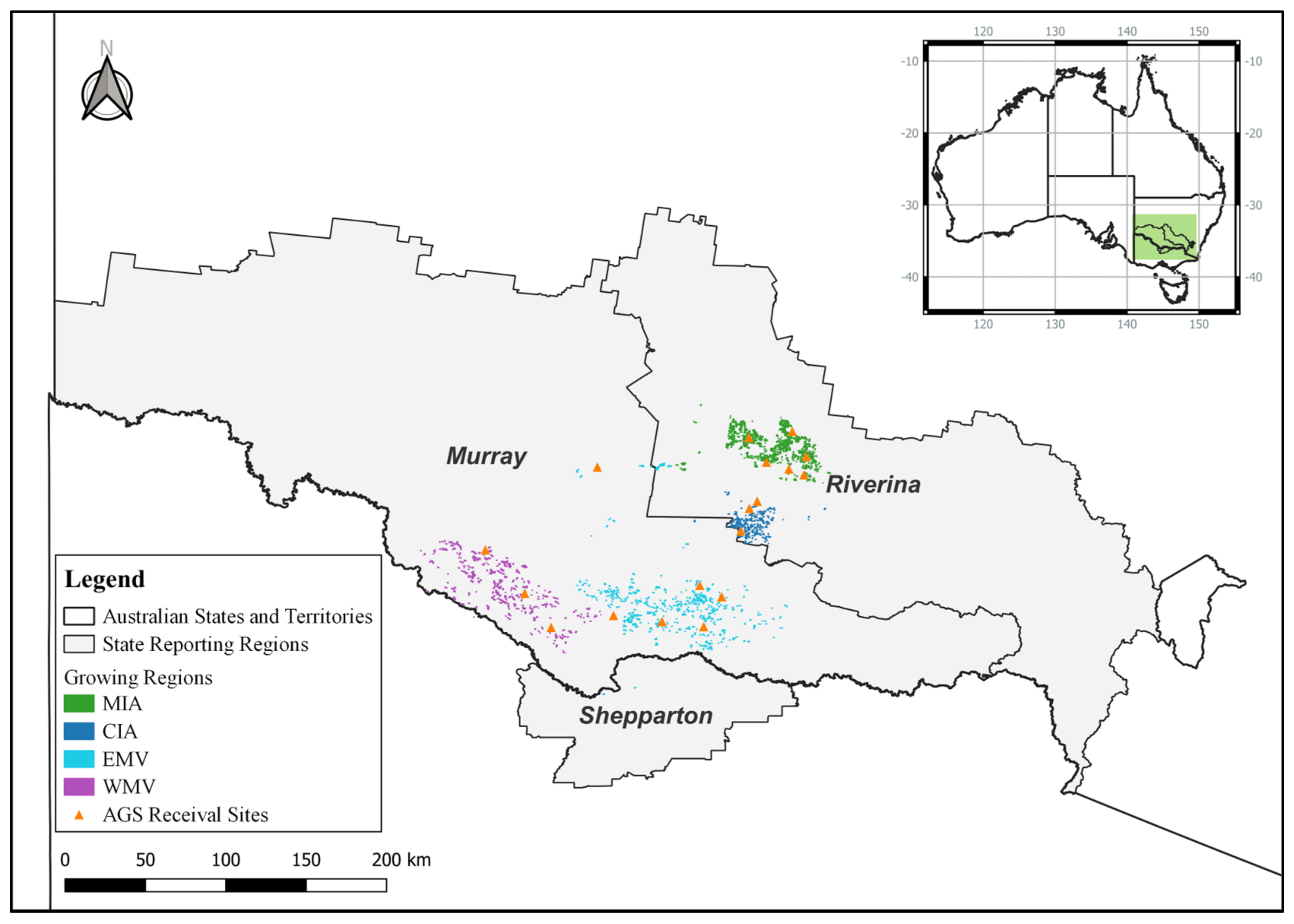
2.1. Study Area
2.2. Datasets and Pre-Processing
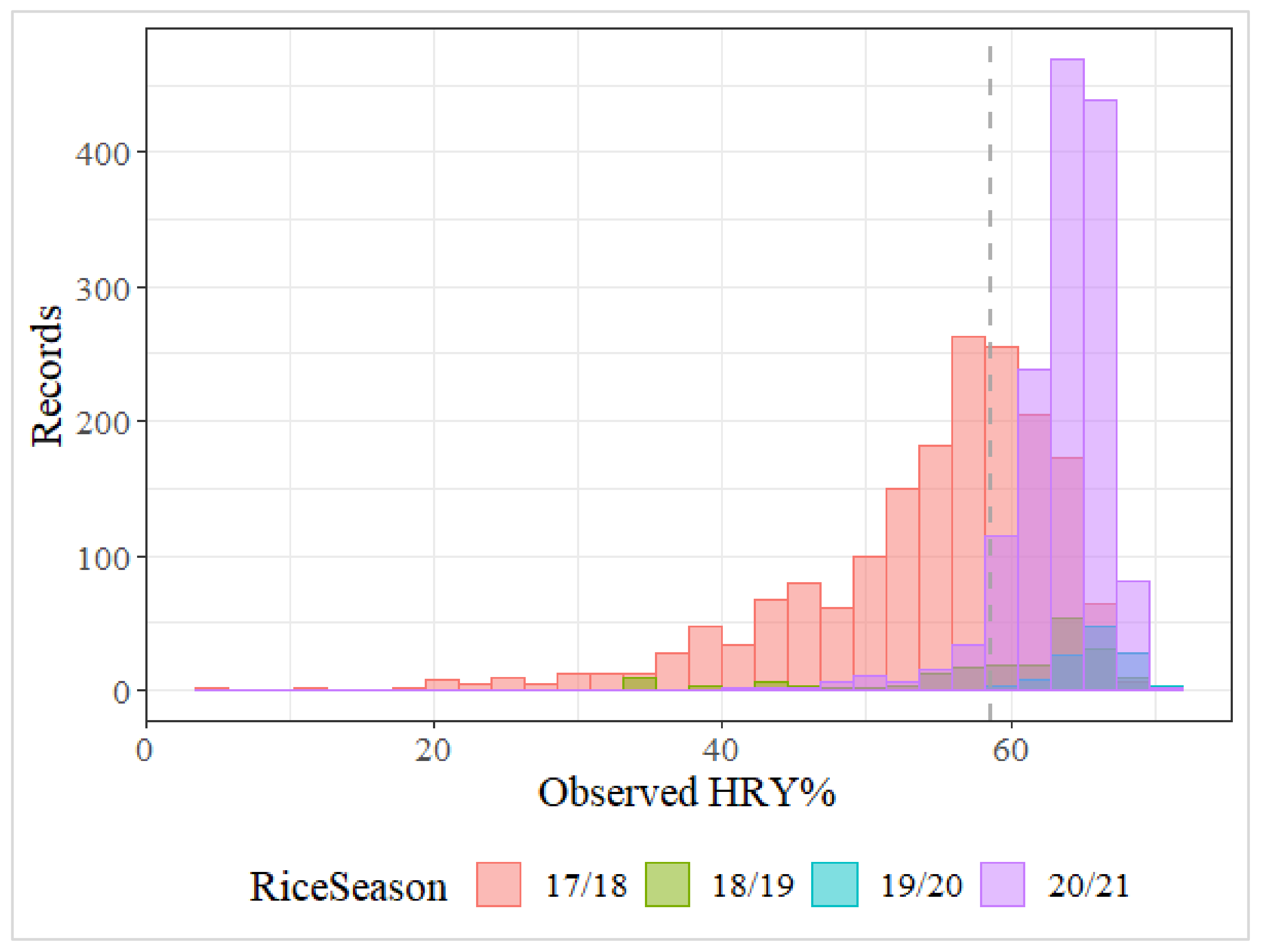
2.2.1. Agronomy
2.2.2. Weather
2.2.3. Soil
2.2.4. Plant Measurements
2.3. Crop Records Feature Engineering
2.3.1. Environmental Feature Engineering
2.3.2. Erroneous Record Filter
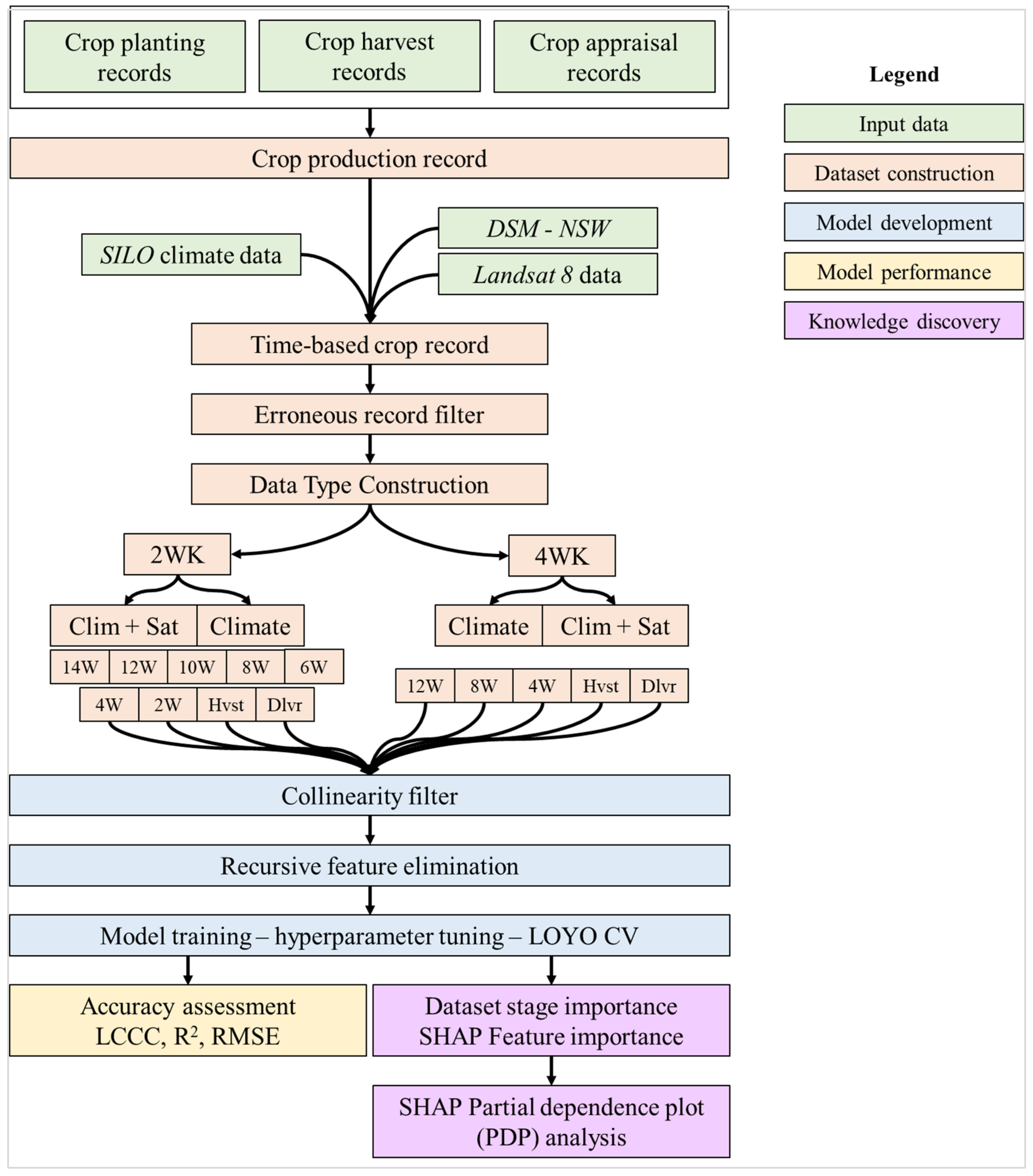
2.4. Model Development
2.4.1. Feature Selection
2.4.2. Machine Learning Algorithm—XGBoost
2.4.3. Experiment Design
2.5. Model Performance
2.6. Knowledge Discovery
3. Results
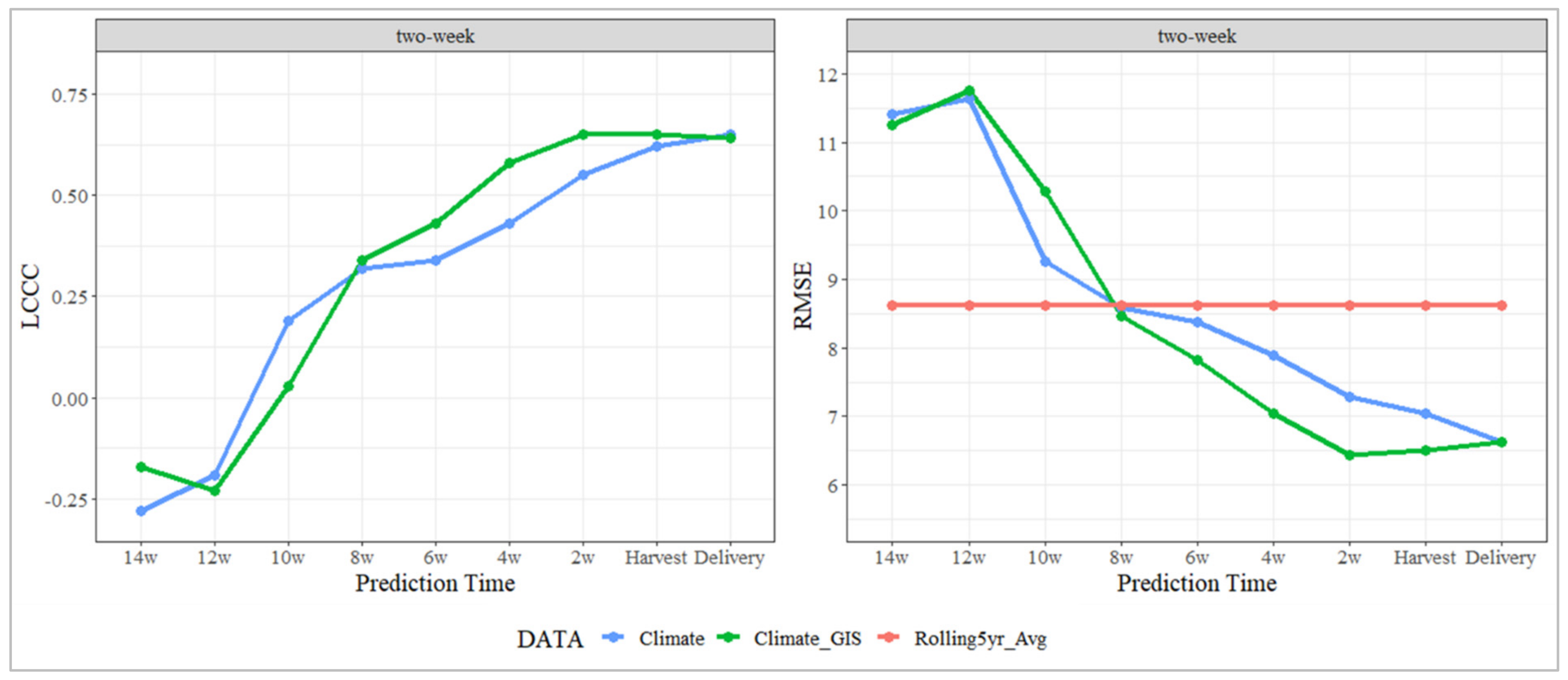
3.1. Model Accuracy
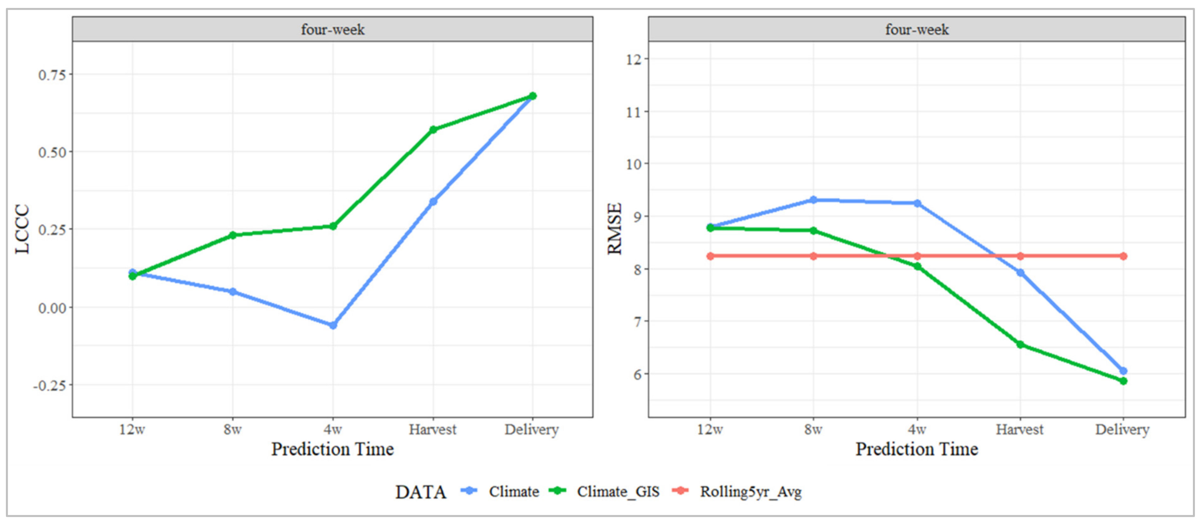
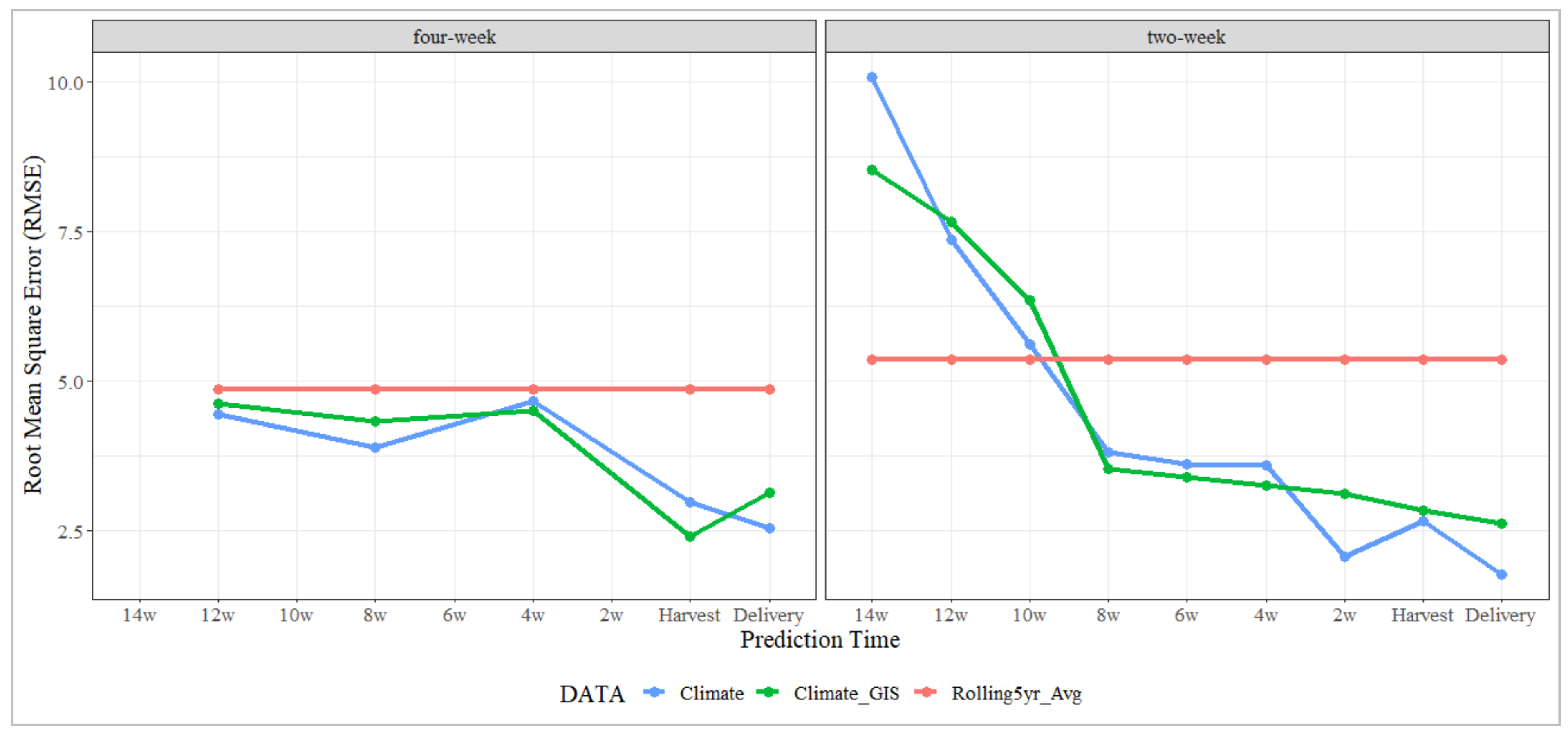
3.1.1. Crop Level Forecast
3.1.2. Season Level Forecast
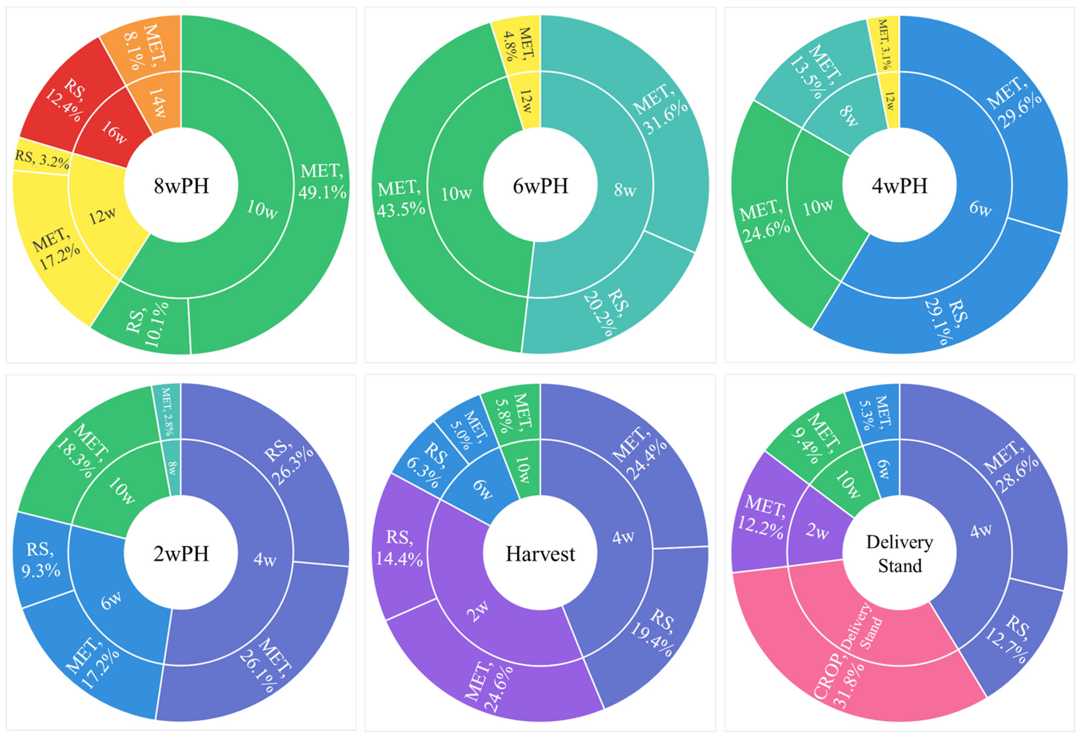
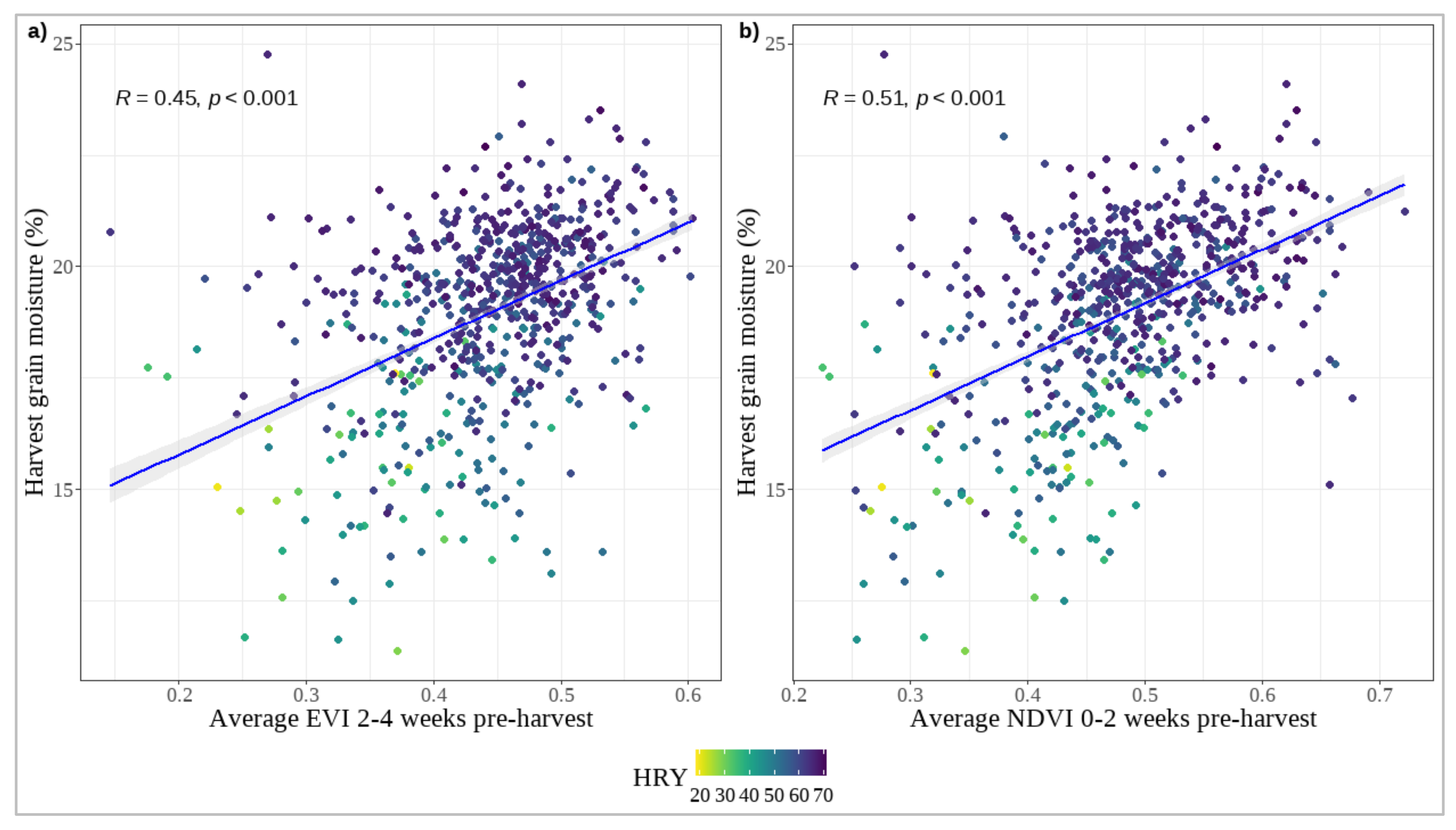
3.2. Feature Importance
4. Discussion
4.1. Model Performance
4.2. Feature Importance
4.3. Industry Applications
4.3.1. Grower Management
4.3.2. Optimisation of Contracts of Milling Fractions
4.4. Limitations
5. Conclusions
Author Contributions
Funding
Data Availability Statement
Conflicts of Interest
References
- Srivastava, A.K.; Safaei, N.; Khaki, S.; Lopez, G.; Zeng, W.; Ewert, F.; Gaiser, T.; Rahimi, J. Winter wheat yield prediction using convolutional neural networks from environmental and phenological data. Sci. Rep. 2022, 12, 3215. [Google Scholar] [CrossRef] [PubMed]
- Vannoppen, A.; Gobin, A. Estimating farm wheat yields from NDVI and meteorological data. Agronomy 2021, 11, 946. [Google Scholar] [CrossRef]
- Donohue, R.J.; Lawes, R.A.; Mata, G.; Gobbett, D.; Ouzman, J. Towards a national, remote-sensing-based model for predicting field-scale crop yield. Field Crops Res. 2018, 227, 79–90. [Google Scholar] [CrossRef]
- Wu, B.; Gommes, R.; Zhang, M.; Zeng, H.; Yan, N.; Zou, W.; Zheng, Y.; Zhang, N.; Chang, S.; Xing, Q. Global crop monitoring: A satellite-based hierarchical approach. Remote Sens. 2015, 7, 3907–3933. [Google Scholar] [CrossRef]
- Chipanshi, A.; Zhang, Y.; Kouadio, L.; Newlands, N.; Davidson, A.; Hill, H.; Warren, R.; Qian, B.; Daneshfar, B.; Bedard, F.; et al. Evaluation of the Integrated Canadian Crop Yield Forecaster (ICCYF) model for in-season prediction of crop yield across the Canadian agricultural landscape. Agric. For. Meteorol. 2015, 206, 137–150. [Google Scholar] [CrossRef]
- Yang, J.; Ouyang, C.; Dik, G.; Corry, P.; ter Hofstede, A.H. Crop Harvest Forecast via Agronomy-Informed Process Modelling and Predictive Monitoring. In Proceedings of the International Conference on Advanced Information Systems Engineering, Leuven, Belgium, 6–10 June 2022; Springer: Berlin/Heidelberg, Germany, 2022. [Google Scholar]
- Feng, P.; Wang, B.; Liu, D.L.; Waters, C.; Xiao, D.; Shi, L.; Yu, Q. Dynamic wheat yield forecasts are improved by a hybrid approach using a biophysical model and machine learning technique. Agric. For. Meteorol. 2020, 285, 107922. [Google Scholar] [CrossRef]
- Keating, B.A.; Carberry, P.S.; Hammer, G.L.; Probert, M.E.; Robertson, M.J.; Holzworth, D.; Huth, N.I.; Hargreaves, J.N.; Meinke, H.; Hochman, Z. An overview of APSIM, a model designed for farming systems simulation. Eur. J. Agron. 2003, 18, 267–288. [Google Scholar] [CrossRef]
- Li, L.; Wang, B.; Feng, P.; Wang, H.; He, Q.; Wang, Y.; Liu, D.L.; Li, Y.; He, J.; Feng, H. Crop yield forecasting and associated optimum lead time analysis based on multi-source environmental data across China. Agric. For. Meteorol. 2021, 308, 108558. [Google Scholar] [CrossRef]
- Filippi, P.; Jones, E.J.; Wimalathunge, N.S.; Somarathna, P.D.; Pozza, L.E.; Ugbaje, S.U.; Jephcott, T.G.; Paterson, S.E.; Whelan, B.M.; Bishop, T.F. An approach to forecast grain crop yield using multi-layered, multi-farm data sets and machine learning. Precis. Agric. 2019, 20, 1015–1029. [Google Scholar] [CrossRef]
- Dhaliwal, J.K.; Panday, D.; Saha, D.; Lee, J.; Jagadamma, S.; Schaeffer, S.; Mengistu, A. Predicting and interpreting cotton yield and its determinants under long-term conservation management practices using machine learning. Comput. Electron. Agric. 2022, 199, 107107. [Google Scholar] [CrossRef]
- Delerce, S.; Dorado, H.; Grillon, A.; Rebolledo, M.C.; Prager, S.D.; Patiño, V.H.; Garcés Varón, G.; Jiménez, D. Assessing weather-yield relationships in rice at local scale using data mining approaches. PLoS ONE 2016, 11, e0161620. [Google Scholar] [CrossRef] [PubMed]
- Bautista, R.C.P.A. Counce. An overview of rice and rice quality. Cereal Foods World 2020, 65, 52. [Google Scholar]
- Lyman, N.B.; Jagadish, K.S.; Nalley, L.L.; Dixon, B.L.; Siebenmorgen, T. Neglecting rice milling yield and quality underestimates economic losses from high-temperature stress. PLoS ONE 2013, 8, e72157. [Google Scholar] [CrossRef]
- Mohan, V.; Ruchi, V.; Gayathri, R.; Ramya Bai, M.; Shobana, S.; Anjana, R.; Unnikrishnan, R.; Sudha, V. Hurdles in brown rice consumption. In Brown Rice; Springer: Berlin/Heidelberg, Germany, 2017; pp. 255–269. [Google Scholar]
- Kealey, L.M.; Clampett, W.S. Production of Quality Rice in South Eastern Australia; New South Wales Department of Agriculture: Orange, Australia, 2000. [Google Scholar]
- Clarke, A.; Yates, D.; Blanchard, C.; Islam, M.Z.; Ford, R.; Rehman, S.-U.; Walsh, R. The effect of dataset construction and data pre-processing on the eXtreme Gradient Boosting algorithm applied to head rice yield prediction in Australia. Comput. Electron. Agric. 2024, 219, 108716. [Google Scholar] [CrossRef]
- Pearce, M.D.; Marks, B.P.; Meullenet, J.F. Effects of Postharvest Parameters on Functional Changes During Rough Rice Storage. Cereal Chem. 2001, 78, 354–357. [Google Scholar] [CrossRef]
- Lee, S.B.; Chung, C.J.; Noh, S.H. Study on the Improvement of Milling Recovery and Performance (V)-Experimental Study on Rice Whitening Performance of Jet-air Abrasive-Type Whitener. J. Biosyst. Eng. 1983, 8, 17–29. [Google Scholar]
- Lapis, J.R.; Cuevas, R.P.O.; Sreenivasulu, N.; Molina, L. Measuring Head Rice Recovery in Rice. In Rice Grain Quality: Methods and Protocols; Springer: New York, NY, USA, 2019; pp. 89–98. [Google Scholar]
- SunRice. Annual Report 2022. 2022. Available online: https://www.sunrice.com.au/book/Annual_Report_2022.pdf (accessed on 5 February 2022).
- Ricegrowers Association of Australia. Submission to the Review of the Rice Vesting Proclamation. 2021. Available online: https://www.rga.org.au/common/Uploaded%20files/2021%20RGA%20-%20Submission%20to%20the%20review%20of%20the%20rice%20vesting%20proclomation%20140821%20Final.pdf (accessed on 5 February 2022).
- Ashton, D.; Oliver, M.; Norrie, D. Rice farms in the Murray–Darling Basin. In ABARES Research Report 16.2; Australian Bureau of Agricultural and Resource Economics and Sciences (ABARES): Canberra, Australia, 2016. [Google Scholar]
- Filippi, P.; Whelan, B.M.; Vervoort, R.W.; Bishop, T.F. Mid-season empirical cotton yield forecasts at fine resolutions using large yield mapping datasets and diverse spatial covariates. Agric. Syst. 2020, 184, 102894. [Google Scholar] [CrossRef]
- Lanning, S.; Siebenmorgen, T.; Counce, P.; Ambardekar, A.; Mauromoustakos, A. Extreme nighttime air temperatures in 2010 impact rice chalkiness and milling quality. Field Crops Res. 2011, 124, 132–136. [Google Scholar] [CrossRef]
- Zhao, X.; Fitzgerald, M. Climate change: Implications for the yield of edible rice. PLoS ONE 2013, 8, e66218. [Google Scholar] [CrossRef]
- Jeffrey, S.J.; Carter, J.O.; Moodie, K.B.; Beswick, A.R. Using spatial interpolation to construct a comprehensive archive of Australian climate data. Environ. Model. Softw. 2001, 16, 309–330. [Google Scholar] [CrossRef]
- Clampett, W.S.; Williams, R.L.; Lacy, J.M. Improvement of Rice Grain Quality. 2004. Available online: https://www.agrifutures.com.au/wp-content/uploads/publications/04-005.pdf (accessed on 10 March 2021).
- NSW Department of Planning and Environment. Digital Soil Maps for Key Soil Properties over New South Wales, Version 2.0. 2022. Available online: https://datasets.seed.nsw.gov.au/dataset/digital-soil-maps-for-key-soil-properties-over-new-south-wales-version-2-0 (accessed on 10 June 2023).
- Li, J.; Chen, B. Global revisit interval analysis of Landsat-8-9 and Sentinel-2a-2b data for terrestrial monitoring. Sensors 2020, 20, 6631. [Google Scholar] [CrossRef]
- Brinkhoff, J. Early-Season Industry-Wide Rice Maps Using Sentinel-2 Time Series. In Proceedings of the IGARSS 2022-2022 IEEE International Geoscience and Remote Sensing Symposium, Kuala Lumpur, Malaysia, 17–22 July 2022; pp. 5854–5857. [Google Scholar]
- Wang, H.; Ghosh, A.; Linquist, B.; Hijmans, R. Satellite-based observations reveal effects of weather variation on rice phenology. Remote Sens. 2020, 12, 1522. [Google Scholar] [CrossRef]
- Madigan, E.; Guo, Y.; Pickering, M.; Held, A.; Jia, X. Quantitative monitoring of complete rice growing seasons using Sentinel 2 time series images. In Proceedings of the IGARSS 2018-2018 IEEE International Geoscience and Remote Sensing Symposium, Valencia, Spain, 22–27 July 2018; pp. 7699–7702. [Google Scholar]
- Bautista, R.; Siebenmorgen, T.; Mauromoustakos, A. The role of rice individual kernel moisture content distributions at harvest on milling quality. Trans. ASABE 2009, 52, 1611–1620. [Google Scholar] [CrossRef]
- Siebenmorgen, T.; Bautista, R.; Counce, P. Optimal harvest moisture contents for maximizing milling quality of long-and medium-grain rice cultivars. Appl. Eng. Agric. 2007, 23, 517–527. [Google Scholar] [CrossRef]
- Nalley, L.; Dixon, B.; Tack, J.; Barkley, A.; Jagadish, K. Optimal Harvest Moisture Content for Maximizing Mid-South Rice Milling Yields and Returns. Agron. J. 2016, 108, 701–712. [Google Scholar] [CrossRef]
- Mzid, N.; Pignatti, S.; Huang, W.; Casa, R. An Analysis of Bare Soil Occurrence in Arable Croplands for Remote Sensing Topsoil Applications. Remote Sens. 2021, 13, 474. [Google Scholar] [CrossRef]
- Ruan, G.; Li, X.; Yuan, F.; Cammarano, D.; Ata-UI-Karim, S.T.; Liu, X.; Tian, Y.; Zhu, Y.; Cao, W.; Cao, Q. Improving wheat yield prediction integrating proximal sensing and weather data with machine learning. Comput. Electron. Agric. 2022, 195, 106852. [Google Scholar] [CrossRef]
- Allen, M.P. Understanding Regression Analysis; Springer Science & Business Media: Berlin/Heidelberg, Germany, 2004; pp. 176–180. [Google Scholar]
- Bocca, F.F.L.H.A. Rodrigues. The effect of tuning, feature engineering, and feature selection in data mining applied to rainfed sugarcane yield modelling. Comput. Electron. Agric. 2016, 128, 67–76. [Google Scholar] [CrossRef]
- Whitmire, C.D.; Vance, J.M.; Rasheed, H.K.; Missaoui, A.; Rasheed, K.M.; Maier, F.W. Using machine learning and feature selection for alfalfa yield prediction. AI 2021, 2, 71–88. [Google Scholar] [CrossRef]
- Ghafarian, F.; Wieland, R.; Lüttschwager, D.; Nendel, C. Application of extreme gradient boosting and Shapley Additive explanations to predict temperature regimes inside forests from standard open-field meteorological data. Environ. Model. Softw. 2022, 156, 105466. [Google Scholar] [CrossRef]
- Obsie, E.Y.; Qu, H.; Drummond, F. Wild blueberry yield prediction using a combination of computer simulation and machine learning algorithms. Comput. Electron. Agric. 2020, 178, 105778. [Google Scholar] [CrossRef]
- Chen, T.C. Guestrin, XGBoost: A Scalable Tree Boosting System. In Proceedings of the 22nd ACM SIGKDD International Conference on Knowledge Discovery and Data Mining, San Francisco, CA, USA, 13–17 August 2016; Association for Computing Machinery: San Francisco, CA, USA; pp. 785–794. [Google Scholar]
- Lin, L.I.-K. A Concordance Correlation Coefficient to Evaluate Reproducibility. Biometrics 1989, 45, 255–268. [Google Scholar] [CrossRef]
- Jones, E.J.; Bishop, T.F.; Malone, B.P.; Hulme, P.J.; Whelan, B.M.; Filippi, P. Identifying causes of crop yield variability with interpretive machine learning. Comput. Electron. Agric. 2022, 192, 106632. [Google Scholar] [CrossRef]
- Molnar, C. Interpretable Machine Learning. 2023. Available online: https://christophm.github.io/interpretable-ml-book/ (accessed on 1 November 2023).
- Clarke, A.; Yates, D.; Blanchard, C.; Islam, M.Z.; Ford, R.; Rehman, S.-U.; Walsh, R. Combining satellite, soil and climate data to predict Head Rice Yield in Australia using machine learning approaches. Artif. Intell. Agric. 2024; manuscript submitted for publication—awaiting first response. [Google Scholar]
- Counce, P.A.; Siebenmorgen, T.J.; Vories, E.D.; Pitts, D.J. Time of draining and harvest effects on rice grain yield and quality. J. Prod. Agric. 1990, 3, 436–445. [Google Scholar] [CrossRef]
- Kunze, O.R.; Peralta, E.; Turner, F.T. Fissured Rice Related to Grain Moisture, Weather and Fertilization Rates; American Society of Agricultural Engineers: St. Joseph, MI, USA, 1988. [Google Scholar]
- Abayawickrama, A.; Reinke, R.F.; Fitzgerald, M.A.; Harper, J.D.; Burrows, G.E. Influence of high daytime temperature during the grain filling stage on fissure formation in rice. J. Cereal Sci. 2017, 74, 256–262. [Google Scholar] [CrossRef]
- Ahmed, N.; Tetlow, I.J.; Nawaz, S.; Iqbal, A.; Mubin, M.; Nawaz ul Rehman, M.S.; Butt, A.; Lightfoot, D.A.; Maekawa, M. Effect of high temperature on grain filling period, yield, amylose content and activity of starch biosynthesis enzymes in endosperm of basmati rice. J. Sci. Food Agric. 2015, 95, 2237–2243. [Google Scholar] [CrossRef] [PubMed]
- Ali, F.; Waters, D.L.; Ovenden, B.; Bundock, P.; Raymond, C.A.; Rose, T.J. Heat stress during grain fill reduces head rice yield through genotype dependant increased husk biomass and grain breakage. J. Cereal Sci. 2019, 90, 102820. [Google Scholar] [CrossRef]
- Huete, A.; Didan, K.; Miura, T.; Rodriguez, E.P.; Gao, X.; Ferreira, L.G. Overview of the radiometric and biophysical performance of the MODIS vegetation indices. Remote Sens. Environ. 2002, 83, 195–213. [Google Scholar] [CrossRef]
- Meroni, M.; Waldner, F.; Seguini, L.; Kerdiles, H.; Rembold, F. Yield forecasting with machine learning and small data: What gains for grains? Agric. For. Meteorol. 2021, 308, 108555. [Google Scholar] [CrossRef]
- Chen, Y.; Tao, F. Potential of remote sensing data-crop model assimilation and seasonal weather forecasts for early-season crop yield forecasting over a large area. Field Crops Res. 2022, 276, 108398. [Google Scholar] [CrossRef]
- Li, Y.; Zeng, H.; Zhang, M.; Wu, B.; Zhao, Y.; Yao, X.; Cheng, T.; Qin, X.; Wu, F. A county-level soybean yield prediction framework coupled with XGBoost and multidimensional feature engineering. Int. J. Appl. Earth Obs. Geoinf. 2023, 118, 103269. [Google Scholar] [CrossRef]
- Cai, Y.; Guan, K.; Lobell, D.; Potgieter, A.B.; Wang, S.; Peng, J.; Xu, T.; Asseng, S.; Zhang, Y.; You, L. Integrating satellite and climate data to predict wheat yield in Australia using machine learning approaches. Agric. For. Meteorol. 2019, 274, 144–159. [Google Scholar] [CrossRef]
- Alcantara, J.M.; Cassman, K.G.; Consuelo, M.; Bienvenido, O.; Samuel, P. Effects of late nitrogen fertilizer application on head rice yield, protein content, and grain quality of rice. Cereal Chem. 1996, 73, 556–560. [Google Scholar]
- Bautista, R.C.; Siebenmorgen, T.J. Rice kernel properties affecting milling quality at harvest. Res. Ser. Ark. Agric. Exp. Stn. 2000, 485, 238–243. [Google Scholar]
- Siebenmorgen, T.; Bautista, R.; Meullenet, J.F. Predicting rice physicochemical properties using thickness fraction properties. Cereal Chem. 2006, 83, 275–283. [Google Scholar] [CrossRef]
- Brinkhoff, J.; McGavin, S.L.; Dunn, T.; Dunn, B.W. Predicting rice phenology and optimal sowing dates in temperate regions using machine learning. Agron. J. 2023, 116, 871–885. [Google Scholar] [CrossRef]
- Brinkhoff, J.; Clarke, A.; Dunn, B.W.; Groat, M. Analysis and forecasting of Australian rice yield using phenology-based aggregation of satellite and weather data. Agric. For. Meteorol. 2024, 353, 110055. [Google Scholar] [CrossRef]
- Boschetti, M.; Stroppiana, D.; Brivio, P.; Bocchi, S. Multi-year monitoring of rice crop phenology through time series analysis of MODIS images. Int. J. Remote Sens. 2009, 30, 4643–4662. [Google Scholar] [CrossRef]
- Brinkhoff, J.; Houborg, R.; Dunn, B.W. Rice ponding date detection in Australia using Sentinel-2 and Planet Fusion imagery. Agric. Water Manag. 2022, 273, 107907. [Google Scholar] [CrossRef]
- Nayak, H.S.; Silva, J.V.; Parihar, C.M.; Krupnik, T.J.; Sena, D.R.; Kakraliya, S.K.; Jat, H.S.; Sidhu, H.S.; Sharma, P.C.; Jat, M.L.; et al. Interpretable machine learning methods to explain on-farm yield variability of high productivity wheat in Northwest India. Field Crops Res. 2022, 287, 108640. [Google Scholar] [CrossRef]

| Category | Variable | Abbreviation | Format | Source | Calculations | Stage Specific |
|---|---|---|---|---|---|---|
| Crop production data | Sowing date | Date (DDD) | SunRice | N | ||
| Sowing method | Text | SunRice | N | |||
| Harvest date | Date (DDD) | SunRice | N | |||
| Season length | Days | SunRice | N | |||
| Average delivery trash | trash_pc | % | SunRice | N | ||
| Average delivery moisture | agm_pc | % | SunRice | N | ||
| Head rice yield | HRY | % | SunRice | N | ||
| Soil data | Clay content | Clay | % | NSW DSM | Average 0–30 cm, Average 30–100 cm | N |
| Maximum temperature | CEC | cmolc/kg | NSW DSM | Average 0–30 cm, Average 30–100 cm | N | |
| Electrical conductivity | EC | dS/m | NSW DSM | Average 0–30 cm, Average 30–100 cm | N | |
| Climate data | Daily rainfall | mm | mm | SILO | Total, Days > 1 mm | Y |
| Maximum temperature | maxt | °C | SILO | Average, 3-day rolling average, maximum, minimum, | Y | |
| 7-day rolling average, maximum, minimum | ||||||
| Minimum temperature | mint | °C | SILO | Average, 3-day rolling average, maximum, minimum, | Y | |
| 7-day rolling average, maximum, minimum | ||||||
| Diurnal temperature range | dtr | °C | SILO | Average, 3-day rolling average, maximum, minimum, | Y | |
| 7-day rolling average, maximum, minimum | ||||||
| Growing degree days | gdd | °C | SILO | Average, 3-day rolling average, maximum, minimum, | Y | |
| 7-day rolling average, maximum, minimum | ||||||
| Vapour pressure | vpd | hPa | SILO | Average, 3-day rolling average, maximum, minimum, | Y | |
| 7-day rolling average, maximum, minimum | ||||||
| Evaporation-Class A pan | evap | mm | SILO | Average, 3-day rolling average, maximum, minimum, | Y | |
| 7-day rolling average, maximum, minimum | ||||||
| Water Deficit Index | wdi | : | SILO | Average, 3-day rolling average, maximum, minimum, | Y | |
| 7-day rolling average, maximum, minimum | ||||||
| Solar radiation | rdn | MJ/m2 | SILO | Average, 3-day rolling average, maximum, minimum, | Y | |
| 7-day rolling average, maximum, minimum | ||||||
| Relative humidity at the time of maximum temperature | rhmaxt | % | SILO | Average, 3-day rolling average, maximum, minimum, | Y | |
| 7-day rolling average, maximum, minimum | ||||||
| Relative humidity at the time of minimum temperature | rhmint | % | SILO | Average, 3-day rolling average, maximum, minimum, | Y | |
| 7-day rolling average, maximum, minimum | ||||||
| Diurnal Humidity Range | drh | % | SILO | Average, 3-day rolling average, maximum, minimum, | Y | |
| 7-day rolling average, maximum, minimum | ||||||
| Evapotranspiration-FAO56 short crop | evtp | mm | SILO | Average, 3-day rolling average, maximum, minimum, | Y | |
| 7-day rolling average, maximum, minimum | ||||||
| Satellite data | Normalized Difference Vegetation Index | NDVI | : | Landsat | First, last, average, maximum, minimum, slope | Y |
| Enhanced Vegetation Index | EVI | : | Landsat | First, last, average, maximum, minimum, slope | Y |
Disclaimer/Publisher’s Note: The statements, opinions and data contained in all publications are solely those of the individual author(s) and contributor(s) and not of MDPI and/or the editor(s). MDPI and/or the editor(s) disclaim responsibility for any injury to people or property resulting from any ideas, methods, instructions or products referred to in the content. |
© 2024 by the authors. Licensee MDPI, Basel, Switzerland. This article is an open access article distributed under the terms and conditions of the Creative Commons Attribution (CC BY) license (https://creativecommons.org/licenses/by/4.0/).
Share and Cite
Clarke, A.; Yates, D.; Blanchard, C.; Islam, M.Z.; Ford, R.; Rehman, S.-U.; Walsh, R.P. Integrating Climate and Satellite Data for Multi-Temporal Pre-Harvest Prediction of Head Rice Yield in Australia. Remote Sens. 2024, 16, 1815. https://doi.org/10.3390/rs16101815
Clarke A, Yates D, Blanchard C, Islam MZ, Ford R, Rehman S-U, Walsh RP. Integrating Climate and Satellite Data for Multi-Temporal Pre-Harvest Prediction of Head Rice Yield in Australia. Remote Sensing. 2024; 16(10):1815. https://doi.org/10.3390/rs16101815
Chicago/Turabian StyleClarke, Allister, Darren Yates, Christopher Blanchard, Md. Zahidul Islam, Russell Ford, Sabih-Ur Rehman, and Robert Paul Walsh. 2024. "Integrating Climate and Satellite Data for Multi-Temporal Pre-Harvest Prediction of Head Rice Yield in Australia" Remote Sensing 16, no. 10: 1815. https://doi.org/10.3390/rs16101815
APA StyleClarke, A., Yates, D., Blanchard, C., Islam, M. Z., Ford, R., Rehman, S.-U., & Walsh, R. P. (2024). Integrating Climate and Satellite Data for Multi-Temporal Pre-Harvest Prediction of Head Rice Yield in Australia. Remote Sensing, 16(10), 1815. https://doi.org/10.3390/rs16101815