Article

Deep Learning-Based Automatic River Flow Estimation Using RADARSAT Imagery

Water Earth Environment Center, National Institute of Scientific Research (INRS), 490 de la Couronne Street, Quebec, QC G1K 9A9, Canada
*
Author to whom correspondence should be addressed.
Remote Sens. 2024, 16(10), 1808; https://doi.org/10.3390/rs16101808
Submission received: 29 March 2024 / Revised: 11 May 2024 / Accepted: 15 May 2024 / Published: 20 May 2024
(This article belongs to the Topic Hydrology and Water Resources Management)

Abstract

:
Estimating river flow is a key parameter for effective water resource management, flood risk prevention, and hydroelectric facilities planning. Yet, traditional gauging methods are not reliable under very high flows or extreme events. Hydrometric network stations are often sparse, and their spatial distribution is not optimal. Therefore, many river sections cannot be monitored using traditional flow measurements and observations. In the last few decades, satellite sensors have been considered as complementary observation sources to traditional water level and flow measurements. This kind of approach has provided a way to maintain and expand the hydrometric observation network. Remote sensing data can be used to estimate flow from rating curves that relate instantaneous flow (Q) to channel cross-section geometry (effective width or depth of the water surface). Yet, remote sensing has limitations, notably its dependence on rating curves. Due to their empirical nature, rating curves are limited to specific river sections (reaches) and cannot be applied to other watercourses. Recently, deep-learning techniques have been successfully applied to hydrology. The primary goal of this study is to develop a deep-learning approach for estimating river flow in the Boreal Shield ecozone of Eastern Canada using RADARSAT-1 and -2 imagery and convolutional neural networks (CNN). Data from 39 hydrographic sites in this region were used in modeling. A new CNN architecture was developed to provide a straightforward estimation of the instantaneous river flow rate. Our results yielded a coefficient of determination (R2) and a Nash–Sutcliffe value of 0.91 and a root mean square error of 33 m3/s. Notably, the model performs exceptionally well for rivers wider than 40 m, reflecting its capability to adapt to varied hydrological contexts. These results underscore the potential of integrating advanced satellite imagery with deep learning to enhance hydrological monitoring across vast and remote areas.

1. Introduction

The accurate prediction and management of stream flows is critical for flood monitoring, providing environmental impact assessments, and watershed hydrologic modeling [1,2,3,4]. The traditional approach for estimating river flows is based upon continuous measurements of river levels (stages) that are fitted to stream flow (discharge) to obtain rating curves. Yet, this approach has its limitations. First, it is difficult to obtain representative measurements of flows in extreme situations because there is no field staff who can go out and take measurements when an extreme event occurs [5]. Second, the stage–flow relationship can be substantially altered when river morphology changes due to erosion or solid inputs. Such changes require new gauging to calibrate the rating curve [1,2].
The rating curve-based method is time-consuming and costly given that it requires the maintenance of flow measurement stations. Furthermore, the spatial distribution of hydrometric network stations is generally sparse, and their distribution is not optimal [6]. Regularly monitored stations are generally located in populated areas, while distant stations in sparsely populated locations have few or no observations. In addition, stations at high latitudes, together with log jams and the dominance of braided gravel-bed rivers, can effectively limit river gauging [4]. As a result, many river sections cannot be monitored by flow measurements and observations. This situation is reflected in the decline of gauging stations, the decrease in their number, and the difficulties encountered in accessing river flow information since the 1980s [7,8,9,10,11,12,13]. The constraints and limitations of instantaneous flow measurement stations affect Canada, which has 9% of the world’s renewable freshwater; thus, alternative flow monitoring approaches with greater spatial coverage and scale are required [6].
For these reasons, during the last few decades, satellite sensors have been considered as a complementary observation source to traditional water level and flow [14,15,16,17,18,19]. These data represent a potential solution to water monitoring problems [20]. Indeed, with the increasing availability of remotely sensed data and repeated, consistent, and global measurements from space-based sensors, the integration of satellite data provides a way to maintain and expand the hydrometric observation network [7]. The precision of flow estimation using remote sensing methods still depends upon the accuracy of estimated parameters that are obtained from satellite sensors either directly (width, slope, and height) or indirectly (velocity and bathymetric depth) [21,22,23,24]. Early applications of satellite data to hydrology involved radar altimeters, viz., Geosat, ERS-1, and Topex/Poseidon satellites [18]. Satellite altimetry was an interesting alternative for recording periodic water level variations. These data were used with in situ observations to derive river discharge [25,26]. Similar studies have continued to expand and refine the capabilities of radar altimetry in flow estimation [27,28,29,30]. Nevertheless, radar satellite altimeters have been confirmed to provide inaccurate results for rivers that are less than one kilometer wide due to signal interference from river banks [25]. In addition, their swath widths are quite narrow (~5 km), which means that many areas are not covered, thereby limiting their application [31]. The temporal frequency of satellite altimeters, which varies between 10 and 35 days, is also a limiting factor. This is an important limitation in water level monitoring and flow estimation, especially since the latter requires continuous and regular data. A recent study [32] explored the estimation of river discharge in the Mississippi River Basin using observed water surface characteristics from satellites and satellite altimetry data. This approach employed the optimized Manning equation for parameters such as surface roughness and channel bathymetry, combining altimetric observations from JASON-2/3 and Sentinel-3A/B satellites with features from the SWOT River Database (SWORD). The results demonstrated reasonable accuracy, illustrating the effectiveness of remote sensing in estimating river flow. However, the study acknowledged several constraints, including the dependence on the precision of remote sensing data and the spatial resolution of these data.
In another study [33], data from the SWOT satellite were used to improve the estimation of discharge in the Saigon-Dongnai estuary, an area complexly influenced by tides. Their methodology, based on simulated SWOT products at a node resolution of 200 m and a Monte Carlo analysis, reduced the root mean square error (RMSE) of the discharge estimation. However, they recognize that estimating discharge in estuarine environments poses particular challenges due to large hydraulic variations and inherent errors in SWOT measurements, highlighting the difficulties of generalizing remote sensing methods without specific adaptations to local conditions.
Many researchers have focused on optical sensors to estimate water flow [9,17,34,35,36,37,38,39]. While conceptually similar to the altimeter method that is described above, measurements that are made with optical sensors are derived by the satellites themselves. Moreover, the variable that is selected to calibrate the rating curve is the flow width. Yet, the signal from optical sensors cannot pass through clouds, which strongly affects the quality of a large quantity of acquired data. Also, optical imagery does not allow the detection of water under dense vegetation cover. Given this limitation, some information is not processed [17].
Faced with these challenges, a recent study [34] proposed an innovative method for estimating daily continuous discharge in ungauged headwaters, using multisource remote sensing data such as high-resolution images from GeoEye-1, WorldView-2 satellites, and Landsat archives. This approach, focused on high-mountain regions like the Tibetan Plateau, relies solely on satellite-observed information, such as river widths derived from images with high spatial resolution, without the need for in situ river discharge measurements. Although promising, this methodology acknowledges several challenges, including uncertainties related to the accuracy of calibration references and optimization algorithms, which may limit the application of such technologies in diverse and complex environments.
Building on the challenges associated with optical sensors, a recent study [35] explored an alternative approach using satellite videos for river discharge estimation. This method utilizes large-scale particle image velocimetry (LSPIV) techniques to estimate river flow. The authors integrated high-resolution topographic data with speed estimates derived from satellite videos. This technique, which uses optical flow algorithms to measure water speed from video sequences, shares similarities with traditional optical sensor approaches but distinguishes itself by potentially overcoming some of their limitations.
The results of their study highlight the effectiveness of advanced remote sensing techniques in complex fluvial contexts. However, despite its successes, this study acknowledges several limitations, including the dependence on clear weather conditions for video capture and uncertainties related to the selection of surface velocity-averaging coefficients. These challenges highlight the potential constraints of applying such technologies in diverse environments.
To overcome these problems, several studies have used radar data to estimate water flow [20,23,29,36,37,38,39]. Indeed, due to the sensitivity of the radar signal to the presence of water and its ability to penetrate clouds and operate independently of weather conditions, these sensors have shown interesting potential for detecting river water surfaces and for monitoring water flow [4,40]. Despite the potential of radar data to estimate water flow, they have a recurring problem, which is related to the level of noise that degrades image quality and makes direct interpretation of hydrological information difficult. Indeed, they all use a proxy for the estimation of flow, especially in terms of the width. Given the noise in radar imagery, the estimation of this proxy is erroneous and, therefore, so is the flow.
In the last two decades, artificial intelligence (AI)-based approaches have been widely used for river flow estimation. For more details, the authors of [41] have prepared a complete review of the application of AI to river flow estimation. In this regard, artificial neural networks (ANNs) are among the most frequently applied models [42,43] given their strong nonlinear adjustment capability. However, ANNs can neither provide an effective representation of the spatial variability of the input data nor extract their characteristics, thereby limiting their applications in practice [44].
Recently, deep-learning techniques have been successfully applied in hydrology and water resource analyses [45,46,47]. Several researchers have shown the potential of deep-learning applications, including classical ANN, in water resource management [48,49], water quality parameter monitoring and estimation [50,51], groundwater loading estimation [52,53], and water level forecasting [54,55]. For example, the convolutional neural network (CNN) is one of the deep-learning algorithms that has been successfully applied to solve water management and hydrological parameter estimation problems [46].
Indeed, the CNN appears to be a promising and appropriate solution to the problems of flow estimation with satellite sensors. The water dynamics and the mechanism that manages the flow are complex and highly nonlinear. Flow estimation depends upon several parameters, including longitudinal and lateral slope, water level, and landform, among others. Given its many stacked layers, the CNN is capable of representing complex and high-dimensional spatial data features [56], together with deducing robust and scalable information, while minimizing the manual intervention rate [57,58,59]. CNNs can also represent nonlinear features while handling raw and noisy data [60].
To overcome the complexity and difficulty of using traditional approaches and to minimize the inconvenience of using remote sensing data and ANN approaches, a CNN network was thus deployed to develop a river flow estimation model. The main objective of this work is to develop a straightforward approach for river flow estimation across the Boreal Shield ecozone of Canada based on a CNN model and Synthetic Aperture Radar (SAR) data.

2. Study Area

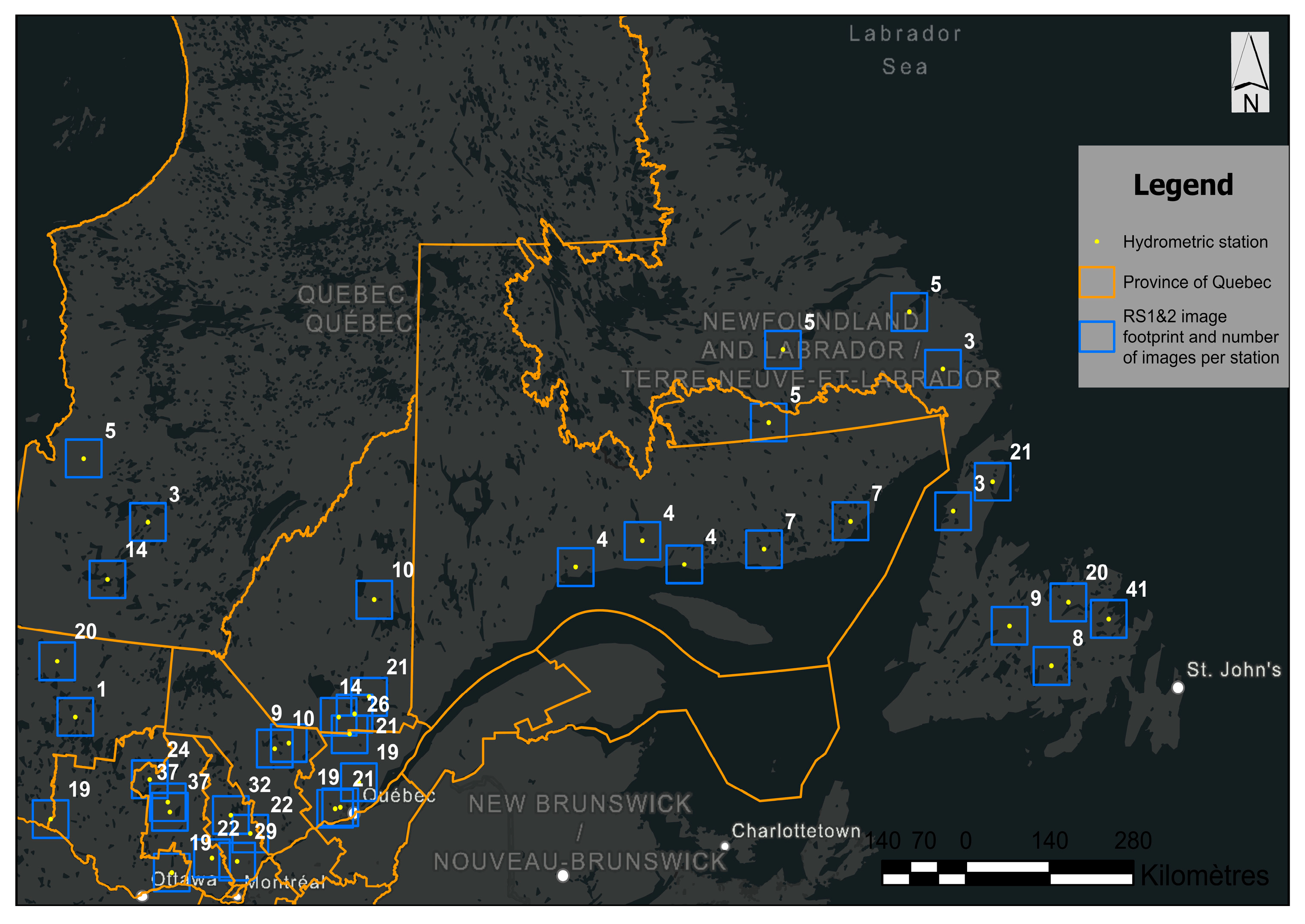
The study area where the research was performed is located in the eastern Boreal Shield ecozone of Canada (Figure 1). The Boreal Shield is the largest terrestrial ecozone in Canada. It covers 1.8 million km2 [61], which is 18.2% of the country’s land base [61]. Several lakes and rivers within the area represent 22% of Canada’s freshwater area. The Boreal Shield ecozone encompasses portions of five provinces: Alberta, Saskatchewan, Manitoba, Ontario, Quebec, and Newfoundland and Labrador [61]. About 30% of the forested area in the eastern ecozone is covered by dense coniferous stands of black spruce (Picea mariana) and balsam fir (Abies balsamea). Mixed coniferous and deciduous forests cover 13%, while open forests cover 35% [62]. The precipitation in this zone is relatively abundant, with 1000 mm falling in the eastern part [63]. The average daily temperature is −10 °C to −20 °C in January and 15 °C to 18 °C in July [63]. The Boreal Shield ecozone is characterized by rocky headlands and rocky lakes. Thus, the most common soil types in the Boreal Shield are wet-climate soils, viz., Brunisols in the west and Podzols in the east, with exposed bare rock and accumulated peats resulting in wetland organic soils, and Gleysols in very swampy areas. The hydrological regime in the eastern part of the Boreal Shield is driven by rainfall and snowmelt [64].

3. Materials and Methods

3.1. In Situ and Satellite Dataset

3.1.1. Satellite Data

RADARSAT-1 and RADARSAT-2 (RS-1 and RS-2) data that were acquired in ascending and descending orbits were used in this study. These sensors emit C-band microwaves (5.6 cm wavelength) at respective frequencies of 5.3 GHz (RS-1) and 5.4 GHz (RS-2). They follow a helio-synchronous orbit and are equipped with a SAR sensor, allowing the acquisition of images with high spatial resolution. The radar backscatter coefficients, which are denoted by sigma0 in the SAR images in this study, are calculated from the Ground-Range-Detected products.
The selected images are in fine acquisition mode, with a spatial resolution of 8 m and HH polarization. A total of 600 images (between 1997 and 2013) were collected and pre-processed to calibrate and validate the river flow estimation CNN model. These images cover all hydrometric stations within the study area (Figure 2).
The data were acquired during summer periods (May to August), with conditions of open water flow without ice or snow. Prior to data analysis, an initial pre-processing of the SAR data was necessary. Indeed, all RS-1 and RS-2 images are orthorectified using orbital parameters and a digital terrain model (PCI Geomatica, PCI Geomatics, Richmond Hill, ON). Radiometric calibration was also applied. This last step allowed an image to be obtained, the pixel value of which really corresponds to the radar backscatter coefficient of the scene. A 3 × 3 Lee SAR Speckle Filter (FLE) was then applied to the correctly orthorectified images to reduce speckles. This filter is available in PCI Geomatica. The final sigma0 image values were subsequently logarithmically transformed to decibels (dB).

3.1.2. In Situ Gauge Dataset

Thirty-nine hydrometric stations (Table A1, Appendix A) that cover the study area were used, including instantaneous flow measurements for the period of 1997 to 2013. These data correspond to the same dates and times of RS-1 and RS-2 images (with an interval of ±1.5 h). They are available for all the selected hydrometric stations. At these stations, river widths vary between 16 and 431 m and instantaneous water flows vary between 0.1 m3/s and 750 m3/s (Table 1).
For the Province of Quebec, data were acquired from the Direction de l’Expertise Hydrique (DEH; ministère de l’Environnement et de la Lutte contre les changements climatiques). The stations that were located in Labrador were obtained from the Environment Canada website.
To provide a comprehensive understanding of the hydrological variability and to contextualize the instantaneous measurements, a historical analysis of flow data from 1983 to 2013 was conducted across the 39 hydrometric stations. This analysis involved examining the average minimum, maximum, and mean annual flow rates based on monthly data. The historical data revealed that minimum average annual flows across the stations ranged from as low as 0.186 m3/s, indicative of small or intermittently flowing streams, to over 912.114 m3/s in larger rivers with substantial catchment areas. Conversely, maximum average annual flows demonstrated even greater variability, with some stations recording flows as high as 4509.83 m3/s, reflecting the capacity of these river systems to experience significant flood events.
These long-term flow data help to identify the range of hydrological conditions encountered across different geographic settings within the study area. A detailed summary of these historical flow rates is provided in Appendix A (Table A1). These supplementary data underscore the variability and complexity of the hydrological regimes within the study area, offering essential insights for the comprehensive analysis of flow dynamics.

3.1.3. Topographic Dataset

Topographic data that were extracted from SRTM digital terrain models (DEMs) at 30 m × 30 m spatial resolution were also used in this study. The data covering the study area were downloaded from the NASA server (https://earthexplorer.usgs.gov, accessed on 1 June 2021) and processed to compute the Height Above Nearest Drainage (HAND).
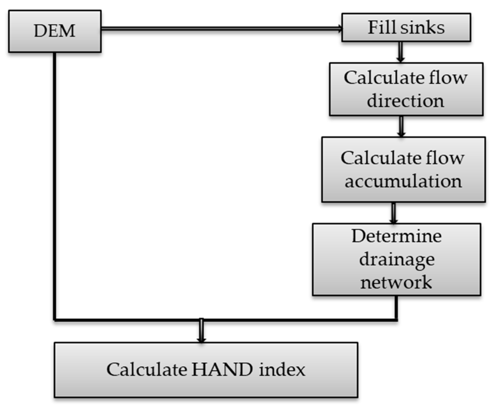
In the HAND model, each point in the watershed is calculated as a function of the elevation above the nearest stream. HAND normalizes the topography to local relative heights that are found in the drainage network [65,66]. The unit of the HAND value is the meter, and it is calculated from the DEM using two steps (Figure 3):
  • Modeling the water flow: to do so, the DEM is first adapted to this objective. Indeed, the DEM contains pits that pose a problem when determining the direction of flow (pits are generally cells surrounded by higher cells). Therefore, the objective is to fill these pits. A hydrologically coherent DEM is thus obtained, which allows the direction of the flow to be defined and to generate an accumulated surface grid. The latter is used to define the drainage network.
  • Generating the nearest drainage map: the data from the local flow direction and the drainage network are combined. Each pixel in the map corresponds to a DEM pixel draining to that pixel. DEM pixels are calculated by calculating their elevational difference from the nearest drainage pixel.
For this work, the HAND product was resampled from 30 m to achieve the same spatial resolution as the radar images (8 m). To perform these steps, the pc raster tool (a library in QGIS) and Jupyter notebook were used to automate the processing.

3.2. CNN Approach to River Flow Estimation

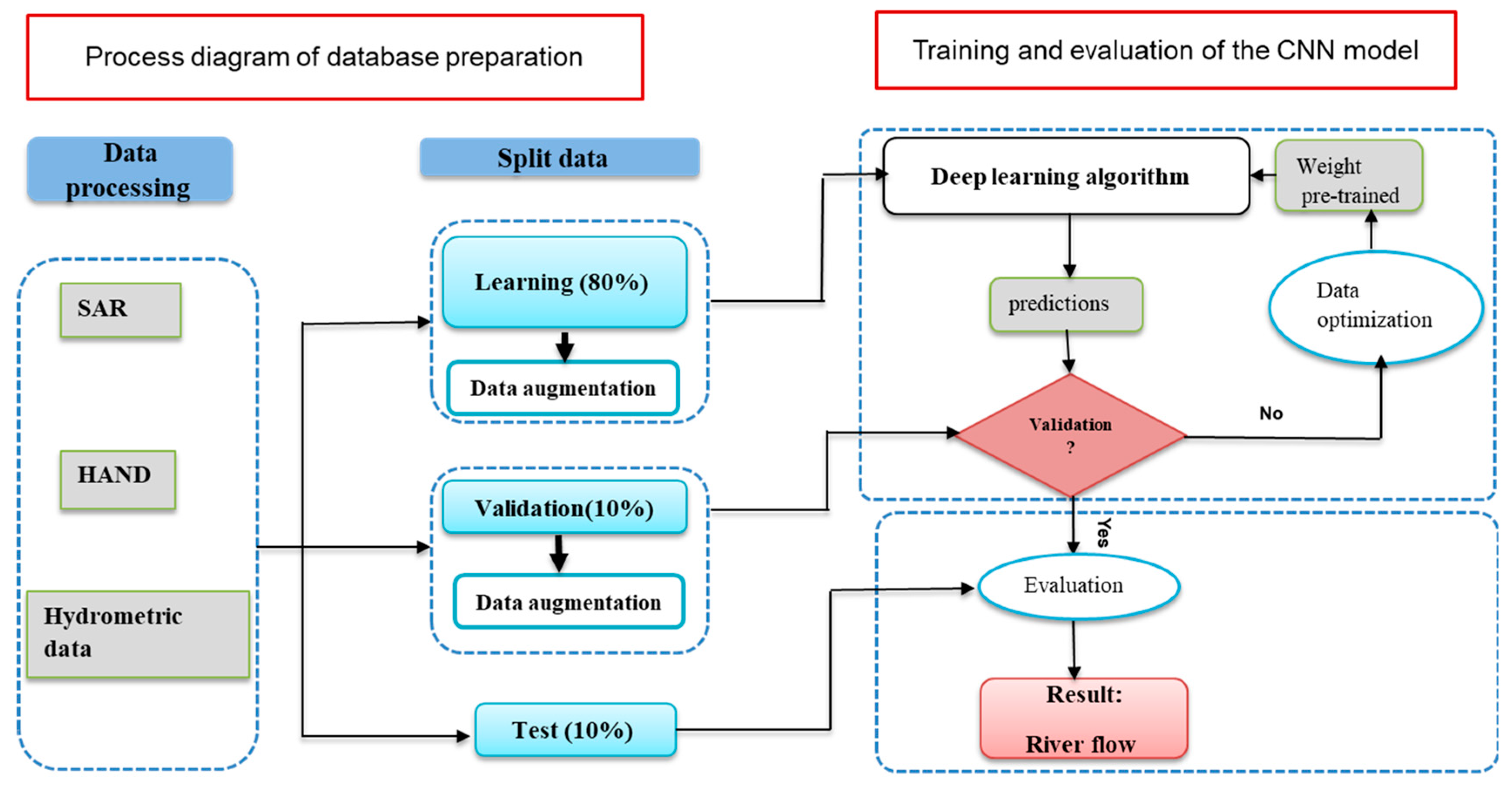
The methodological approach involves two main components (Figure 4). The first part consists of presenting the database that served as input data for the CNN model, while the second part focuses on the training and evaluation of the deep-learning model.

3.2.1. Input Data Pre-Processing

In order to train a CNN algorithm, it is necessary to separate the data into different sets: a training dataset that is used for calibration and adjusting weights; validation datasets that are used to evaluate the model at each calibration iteration; and a test dataset that is completely independent, which is used to measure the model’s accuracy and evaluate its performance. The optimal ratio that was used to split the data is as follows: 80% for training; 10% for validation; and 10% for testing. The choice of ratio was based on several trials. Different ratios were tested to find the best balance between the optimal use of data for model training and the reliable evaluation of model performance. The aforementioned ratio showed the best performance in the tests.
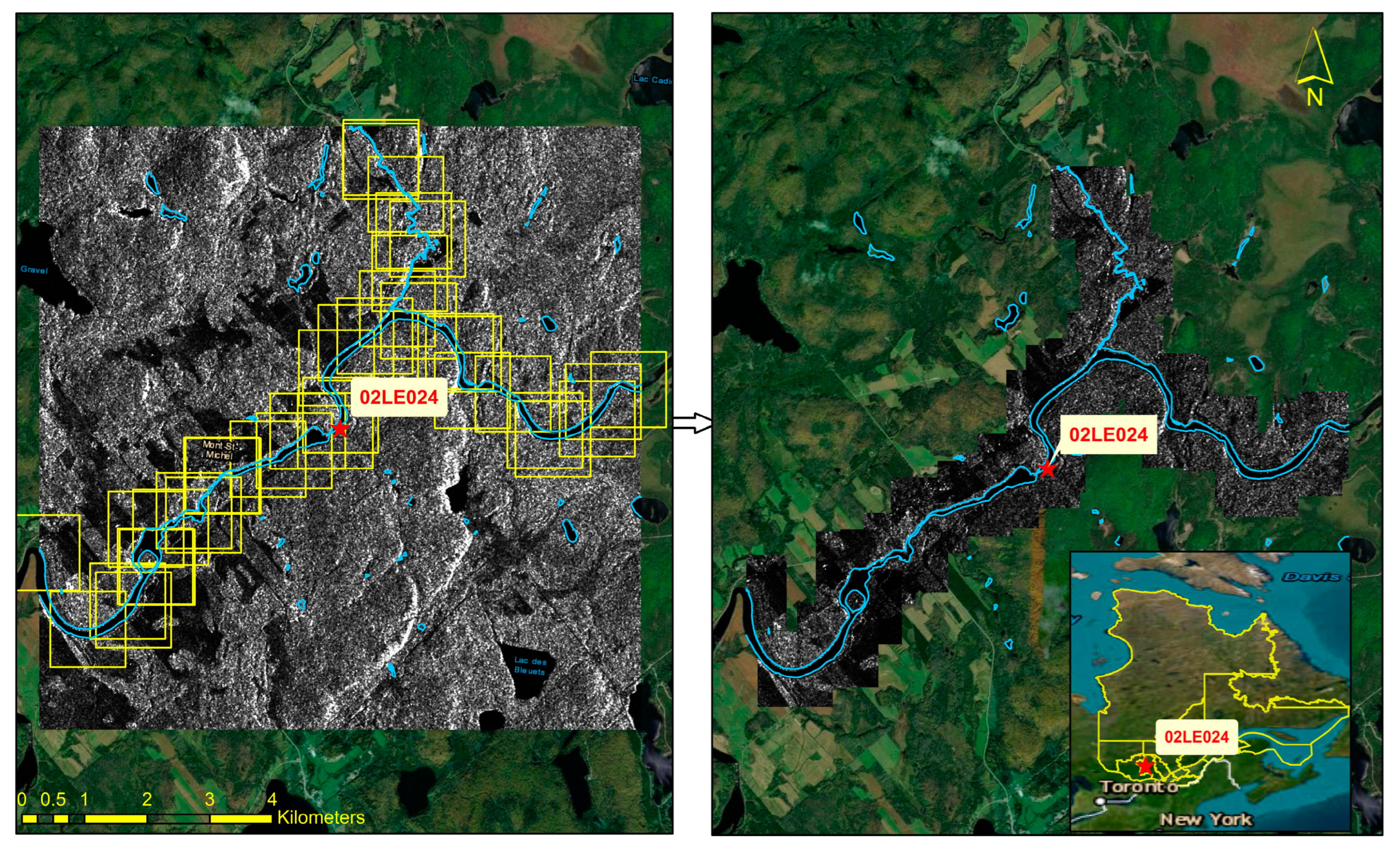
The input data that were considered for this approach are the SAR data and HAND. A series of pre-processing steps were performed on these data. First, a clipping step was applied to the data (Figure 5). In a 5-km buffer zone around the hydrometric stations, the radar images were clipped into small thumbnails along the one-kilometer-wide rivers. The same flow value was assigned to all patches. This increased the number of thumbnails for the model training step. The size of the database was increased from 600 images to 10,000 images.
Once the clipping of the images was completed, normalization of the patches (Equation (1)) was performed. This second step is important because it allows the input data to be standardized to the model as well as obtaining unit variance (1). Therefore, variability within the data is reduced, thereby ensuring a more stable training phase.
Normalization is calculated as follows:
z = x x m i n x m a x x m i n
where z represents normalized pixel values, x is the pixel value before normalization, and x m a x   and   x m i n are the maximum and minimum pixel values.
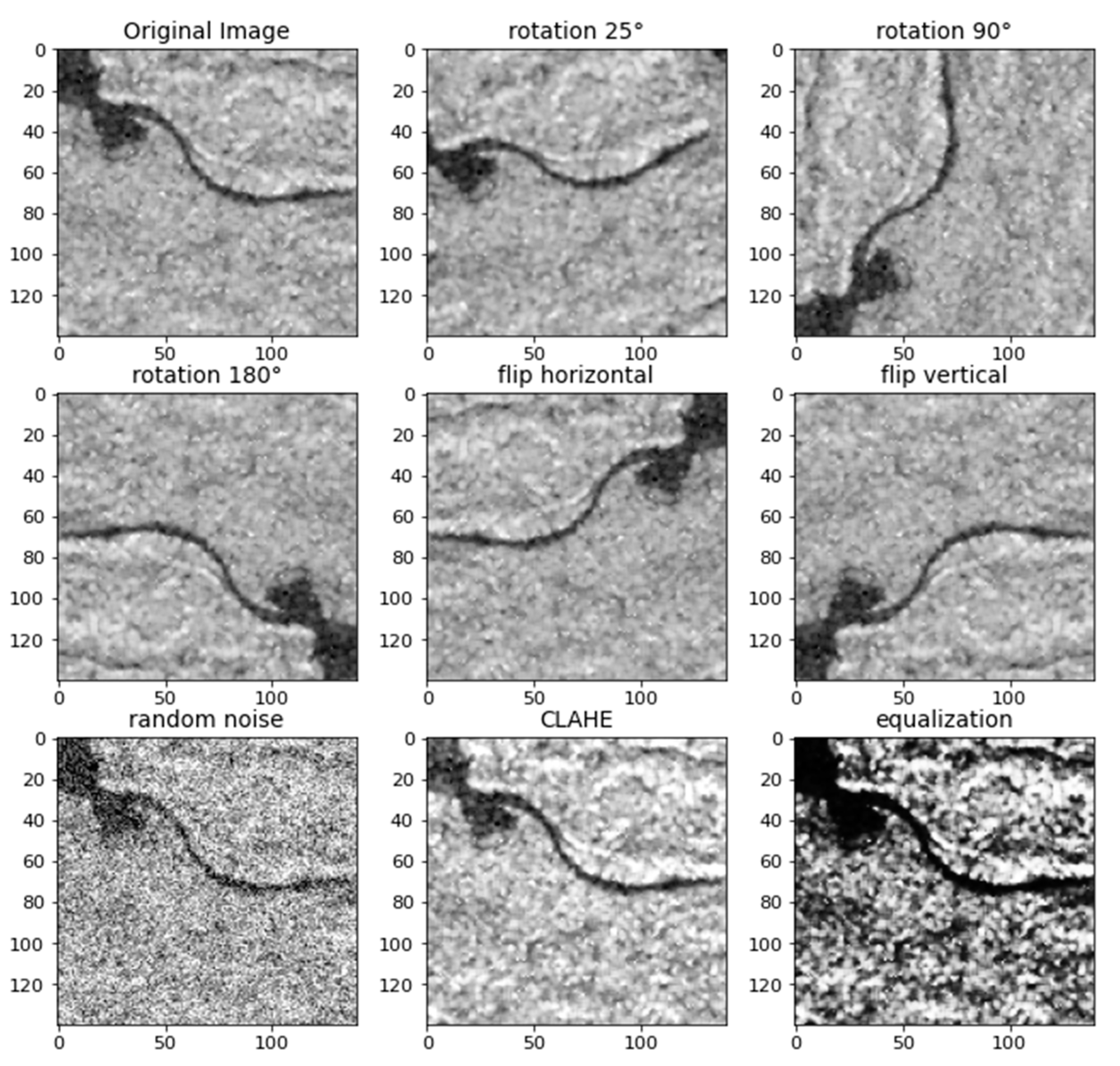
To handle the problems of over-fitting, data augmentation was applied. Over-fitting occurs when the model fits perfectly with the training data, but it estimates poorly with new data. This means that the model trains well on the training data but is not sufficiently generic with other data. Data augmentation is a simple but effective method that reduces over-fitting and contributes to improving the performance of the model [67]. This step allows the quantity of data to be increased by modifying the data that are already available. In this work, each thumbnail received a series of geometric and pixel transformations (Figure 6). For the geometric transformations, different kinds of rotations {25°, 90°, and 180°} were applied. This helped the model to learn the invariant orientation of a channel. Vertical and horizontal flips were also applied. For the pixel transformations, a noise layer was added. Gaussian noise was generated using a separate layer called GaussianNoise. Two adaptive filters, i.e., contrast-limited adaptive histogram equalization (CLAHE) and equalization, were also applied to each thumbnail to increase the contrast and improve the visibility of the edges. They allow the grey level of the image to be changed while preserving its details. These different transformations were performed with the Keras library. Following these transformations, the total number of patches in the database increased from 10,000 to 82,000.

3.2.2. Training and Evaluation of the Deep-Learning Model

In this second section of the methodological approach, the CNN model and the loss function will be explained. For CNN model development and through its different layers, the data will be transformed and will have a new presentation. The last CNN layer will be used to estimate the water flow value. Due to a loss function or cost function, which, in this work, is the mean square error (MSE) (which measures the performance of the algorithm, as shown in Equation (2)), this estimated value will then be challenged with the validation data (the real data value). This will allow a loss score to be computed, which indicates the error difference between estimated and true values. If the error difference is large, an optimization function will be used to adjust the weights and minimize the error difference. Backpropagation is the most commonly used technique [68] for calculating the gradient of the error function relative to one weight at a time. For updating weights and minimizing error variance, stochastic gradient descent algorithms or their variants are commonly used, such as AdaGrad, RMSprop, and Adam. The Adam algorithm was chosen for this work [69].
The input data will then be exposed again to the CNN with adjusted weights. The above steps will be repeated until a minimum error difference between the predicted and true values is obtained (Figure 4). It may be that the best accuracy reached after training is not considered to be sufficient. In this case, modifications of the developed architecture are necessary. This means modifying, especially the parameters, or adding/removing layers in order to find an architecture that correctly models the dataset in question.
M S E = 1 n i = 1 n Q i o b s Q i e s t i m 2
where n is the sample size and Q i o b s   a n d   Q i e s t i m are the observed and estimated flows, respectively.

3.2.3. Proposed CNN Architecture

The typical structure of a CNN consists mainly of an input layer, hidden layers, and an output layer [70]. Hidden layers of a CNN are composed of convolutional layers, a nonlinear layer (also called the activation function [56]), pooling layers [71], and fully connected layers [72].
The input layer allows input data of the entire CNN to be easily manipulated without destroying the internal structure of the latter. Generally, it represents the pixel matrix of the image.
The hidden layers are composed of convolutional layers that extract features from the input images of the previous layer. The results are transmitted to the next layer. This is achieved by using a filter that scans the entire input image and calculates the convolution product between the weights of the convolutional neuron (filter) and each portion of the scanned image. The convolution step is usually followed by a nonlinear transfer operation. The nonlinear layer is also called the activation function. This is an essential element in the neural network given that it introduces nonlinearity into the model. The ReLU (Rectified Linear Activation) function, the sigmoid function, and the hyperbolic tangent function are some of the most commonly used activation functions in deep learning. In this work, the ReLU function was used. The latter allows negative values to be avoided at the output of the neuron. It sets all negative values to zero, while the positive values remain unchanged. ReLU layers have been shown to work much better than other functions [73]. The advantage of ReLU over the others is that it allows for better generalization. It also allows the network to train much faster. Furthermore, it helps to avoid the problem of gradient vanishing. Through the use of the pooling layer, the calculation is reduced and simplified by retaining only the most important features that are present in the input images. In the fully connected layer, the output of the convolution and pooling layers represents the input. This layer connects to all the features of the previous layer to obtain the final output (river flow estimation). In this work, the Global Average Pooling (GAP) layer approach was used instead of fully connected layers. GAP layers are a pooling operation designed to replace fully connected layers [74]. The idea here is to reduce the dimensionality of a tensor that will have a dimension of 1 × 1 × d instead of a size of h × w × d (h: height; w: width; and d: depth). Therefore, GAP layers allow each h w feature map to be reduced to a single number while taking the average of all h w values. Among the advantages of using GAP layers is that there are no parameters to optimize during this step, which helps avoid the over-fitting problem. For more information on the design of CNN structures, see [75,76].
In the output layer, a model’s ability to make predictions depends upon the type of activation function that is being used. Indeed, the linear function has often been used in regression models. Since this work is aimed at estimating river flow, the activation function at the last output layer of this CNN model was defined as a linear function.
To improve training generalization and to avoid over-fitting, the dropout layers technique [77] was used. The idea behind this technique amounts to disabling several nodes at each iteration of the learning process. This alteration forces the network to be redundant and to have alternative paths to correctly predict the output. This helps to reduce the over-fitting problem. This method seemed to be the most suitable for this work, especially since it is extremely light in terms of computational requirements.
The learning rate is a very important parameter that influences the performance of the model. If the learning rate is very low, over-fitting can occur [78]. A high learning rate can lead to oscillations around global minima without reaching it. Therefore, different learning rates were tried in the context of this work. It was found that the CNN model worked best at a learning rate of 10−4.
The most difficult, but also the most important, step is to identify the best-performing architecture that achieves the best flow estimates. Indeed, hyper-parameters need to be adjusted, and there is no single rule that can be applied to the dataset. Several adjustments should be made in order to find the appropriate set of hyper-parameters, thereby maximizing the performance of the model.
Figure 7, together with Table A2 and Table A3 (Appendix A), shows the best design in terms of the number of layers that are used and the values of the hyper-parameters, which are appropriate for the input data. This architecture is the result of many trials and tests. In total, 3,536,617 parameters were trained by the final version of this model.

3.2.4. Model Libraries

The criterion for choosing a deep-learning library is based on its ease of handling, its flexibility (i.e., the type of architecture supported and the possible operations), and also its free and open-source status. The Keras library [79] satisfied all three criteria and was thus selected for this work. It is well suited for developing one’s own models due to its simplified coding. Other libraries that are used for data importation, pre-processing, and visualization are Pandas, NumPy, Scikit-Learn, and PyLab. The Spyder package from Anaconda is used as an interface.
The model training platform that was used is a Deep Learning EC2 instance of Amazon Web Services (AWS), featuring up to eight Gaudi accelerators, 256 GB of high-bandwidth memory, and 768 GB of system memory.

3.2.5. Evaluation of Model Performance

The statistical performance indices that were chosen are coefficient of determination (R2), root mean square error (RMSE), and Nash–Sutcliffe efficiency (NSE). The R2 is a statistical measure that assesses the degree to which a model explains variances in measured flows. RMSE reflects the standard deviation of the residuals (prediction errors). A model’s predictive power is evaluated using the NSE. It allows comparisons between situations with different orders of magnitude of flows [80].
R 2 = i = 1 n Q i o b s μ o b s Q i e s t i m μ e s t i m i = 1 n Q i o b s μ o b s 2 i = 1 n Q i e s t i m μ e s t i m 2 2
R M S E = 1 n i = 1 n Q i o b s Q i e s t i m 2
N S E = 1 i = 1 n Q i o b s Q i e s t i m 2 i = 1 n Q i o b s μ o b s 2
where n is the sample size, Q i o b s   a n d   Q i e s t i m are the observed and estimated flows, respectively, μ o b s is the average of observed flows, and μ e s t i m is the average of estimated flows.

4. Results

4.1. Analysis Based on Input Data

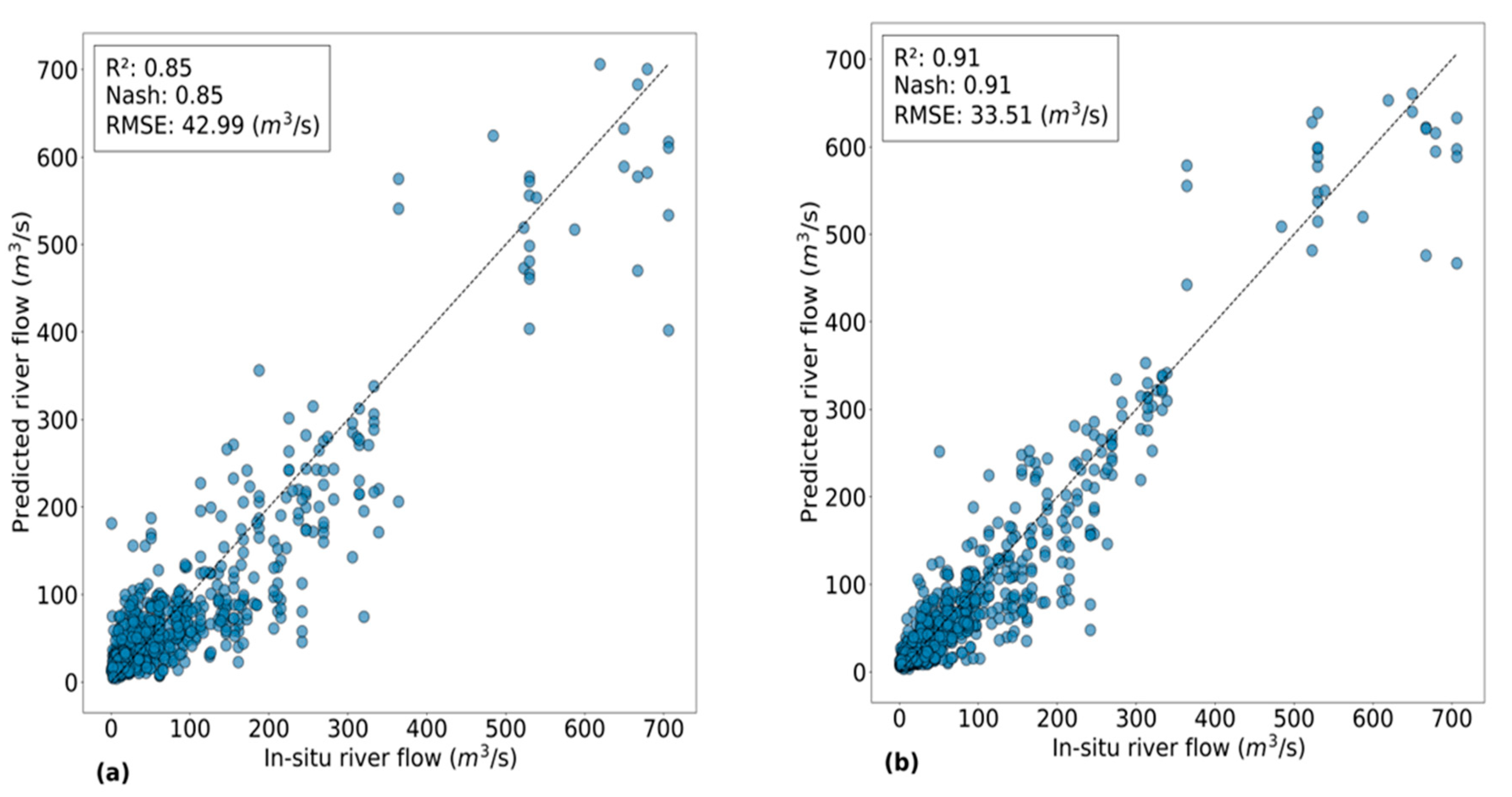
First, the CNN model was trained using only the SAR images. The HAND data were added to the SAR images to train another CNN model for the purposes of comparison. Figure 8 summarizes the CNN training results that were obtained using the SAR data alone and the SAR data with the HAND data. This figure illustrates the relationship between the in situ flow measurements and predicted flow measurements.
SAR images with HAND as input data led to better training of the CNN for flow estimation with R2 = NSE = 0.91 and RMSE = 33.51 m3/s. Flow estimation using SAR data only as input data was less successful, with R2 = NSE = 0.85 and RMSE = 42.99 m3/s.
It should be noted that the rest of the analyses focus only on the results obtained using the CNN model that was trained using the SAR images with HAND data.
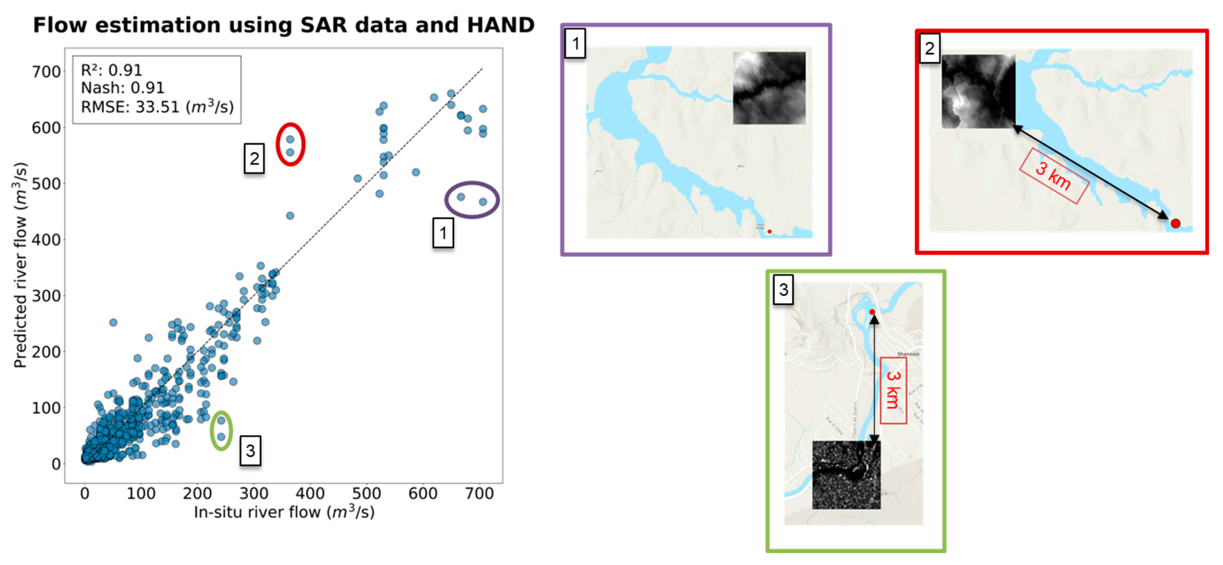
Figure 9 illustrates some examples of flow estimates that are over- or underestimated. Their corresponding images were selected and visually inspected. For three selected examples, the distance between the image and the hydrometric station is large (about 3 km). For image (1), HAND was calculated on a different tributary from the one in which the station is located.

4.2. Analysis According to the Morphometric Characteristics of the Estimation Site

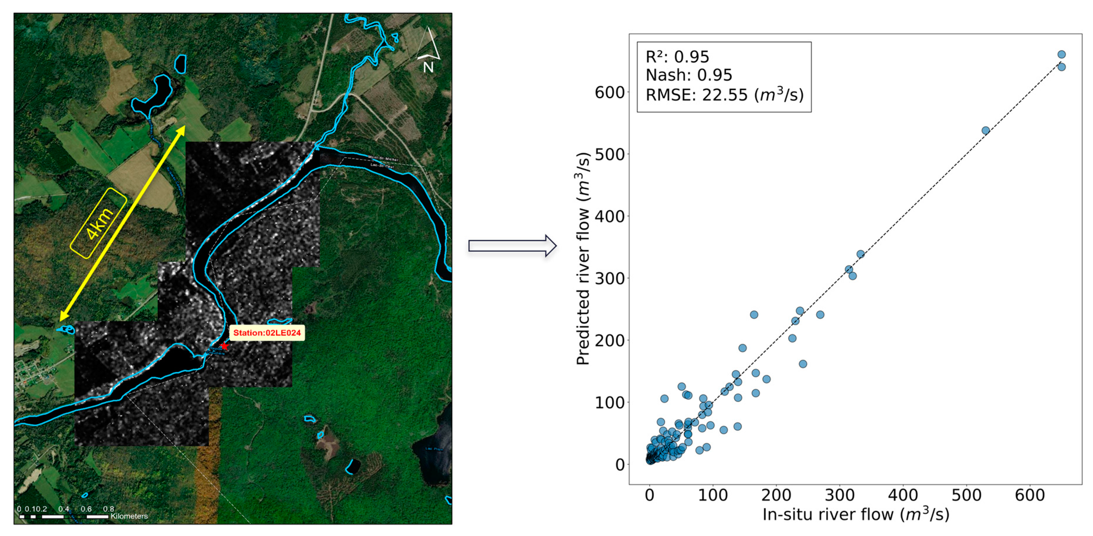
For this analysis, the amount of test data was reduced. Only images taken within a 2-km buffer around the hydrometric station were considered. The goal is to highlight the effects of changing distance from the hydrometric station on flow estimates. Figure 10 shows the relationship between observed and estimated flows following the reduction in distance to the hydrometric station. Compared to previous results, it should be noted that the use of images that are within the 2-km buffer zone around the hydrometric station attained better estimates of river flow. Values of R2, RMSE, and NSE increased to 0.95, 22.55 m3/s, and 0.95, respectively. The scatter plot became increasingly less dispersed with respect to the 1:1 line.
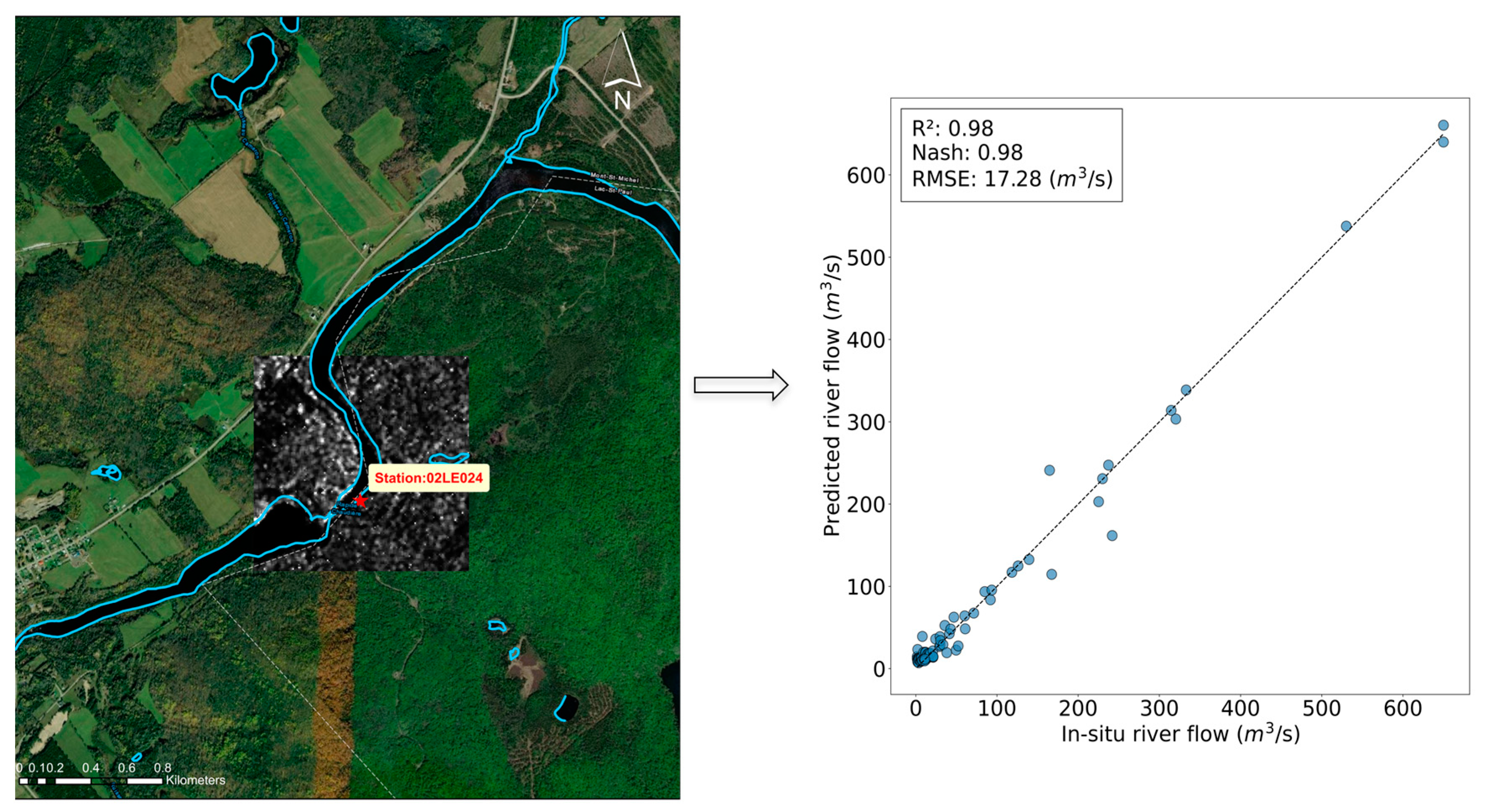
The same test was repeated, except that this time, only the images that passed through the station were considered. Flow estimation results likewise improved, as shown in Figure 11. R2 and NSE values increased from 0.91 with all test data to 0.98. RMSE was reduced from 33.51 to 17.28 m3/s. Thus, it is clear that proximity is a key factor in accurate flow estimation. The closer to the hydrometric station, the better the flow prediction becomes.

4.3. Analysis by Individual Stations of the Flow Estimate

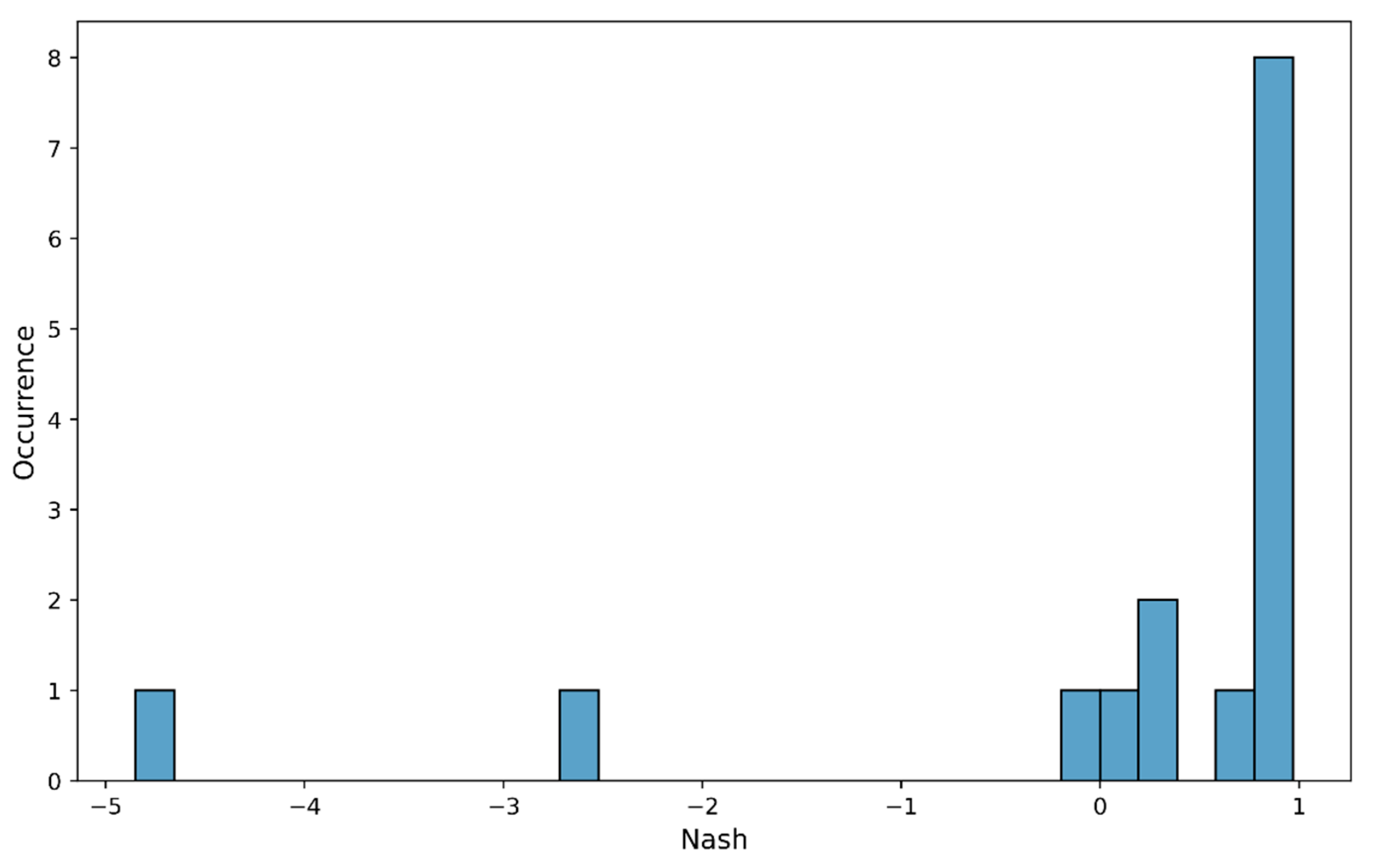
This part aims to analyze how the model estimates flow on different dates with different flow conditions within the same hydrometric station. Among the test data that pass through the hydrometric station, those that have flow observations on different dates were taken. A station-by-station analysis was performed. In total, 15 hydrometric stations were analyzed.
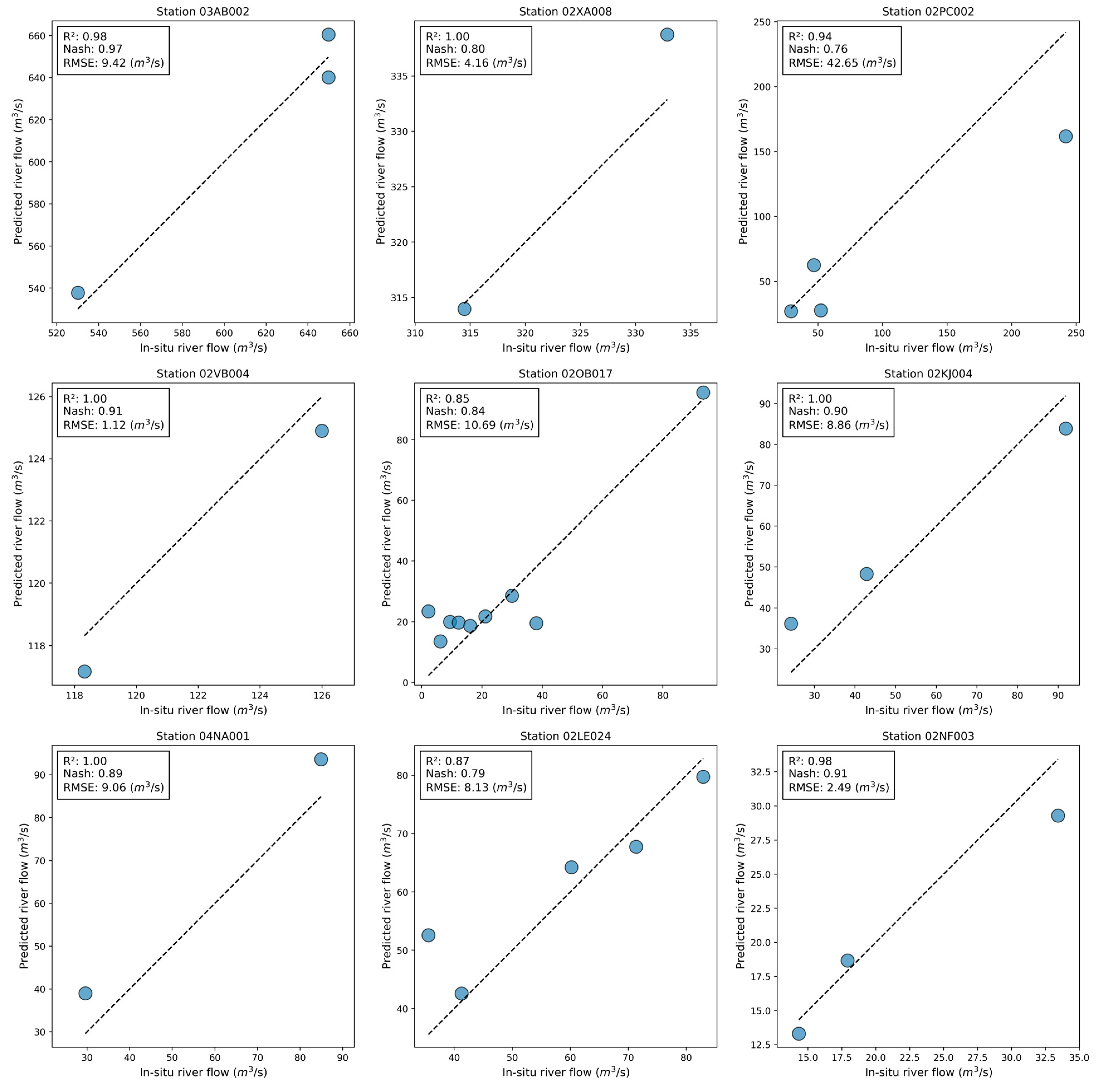
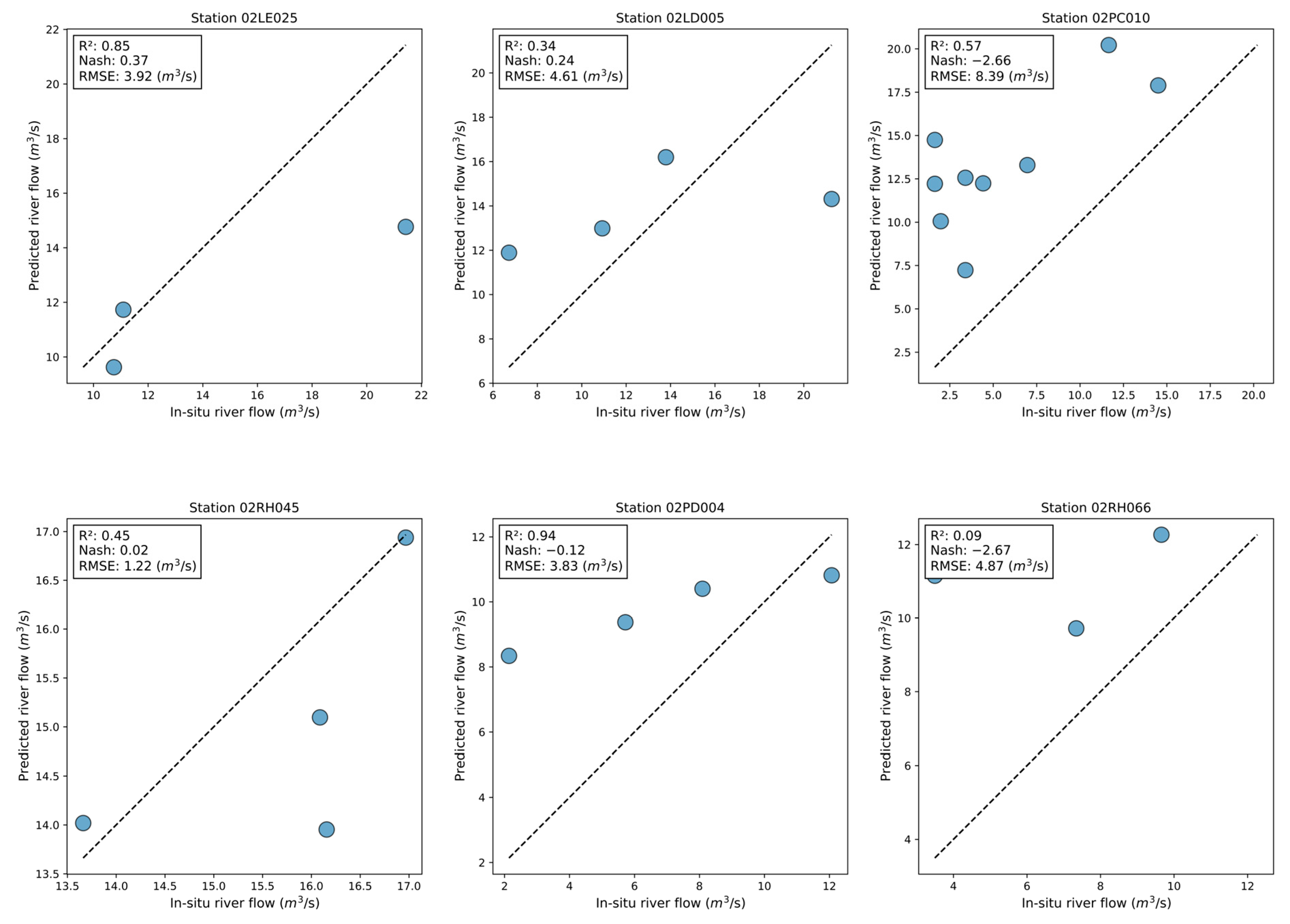
At first inspection, the two performance groups are quite distinct. The first group of flow estimates is characterized by very good performance, while the second group shows less or mediocre performance (Figure 12). Following analysis, it emerged that rivers with widths of 40 m and more belong to the first group, and vice versa. For the stations belonging to the first group of rivers, R2 and NSE vary between 0.79 to 1.00 and 0.76 to 0.97, respectively, and RMSE varies between 2.49 and 42.65 m3/s (Figure 13 and Figure 14). For stations in the second group, R2 and NSE range from 0.06 to 0.85 and −4.85 to 0.37, respectively, while RMSE ranges from 1.22 to 8.39 m3/s. This shows that the model is capable of estimating the flow at the station itself, with different flow conditions, when the width of the river is greater than 40 m.

5. Discussion

Based on the improvements observed in Section 4.1, where the CNN model incorporating the HAND data demonstrated enhanced performance (R2 = NSE = 0.91 and RMSE = 33.51 m3/s) compared to using SAR data alone (R2 = NSE = 0.85, RMSE = 42.99 m3/s), it is clear that adding the topographic aspect significantly augments the model’s ability to estimate in-river flow. This improvement is especially notable for flow values below 300 m3/s, where the results show less dispersion of predicted values around the 1:1 line as visualized in Figure 8.
On one hand, SAR data have been shown to be very useful for mapping the water surface of rivers and tracking change in its width in several studies [7,40,81]. On the other hand, these data exhibit several inconvenient features. Among these is the land effect, which makes it difficult to map water because of shadow regions in the land that have similar values to those over water bodies. The use of the elevation data that are acquired directly by the DEM does not always improve the mapping of the water surface. Yet, because all DEMs contain errors, the simple thresholding in elevation to delimit shadows and water bodies becomes unreliable when the shadows occur in low areas. For this reason, it is necessary to use another land variable that has a strong link with the presence of water and that can overcome the drawbacks of the DEM, such as the HAND. One of the key features of HAND is its ability to determine local drainage potentials and to calculate the elevation of each point in the watershed above the stream closest to its drainage direction [66]. With the HAND data, we are interested in relative spatial changes in elevation rather than height in terms of the absolute value, making the elevation error on the DTM less important. The use of HAND allowed for better delineation of water bodies and, therefore, improved flow estimation.
Indeed, several studies have shown a strong correlation between river width and flow [82,83]. River width information can include the hydraulic geometry of the channel in which an increase or decrease in water extent results in a significantly higher or lower flow. Thus, the proper delineation of water body boundaries is a key step in estimating river flow. The enhanced delineation achieved by combining SAR and HAND data facilitates more reliable flow estimations, enabling the CNN model to better train and predict river flow dynamics, as seen in the improvements documented in Section 4.1.
In sum, the use of SAR images, in conjunction with HAND data, not only addresses the drawbacks of using SAR alone but also significantly enhances the model’s training effectiveness and predictive accuracy for river flow estimation.
In the discussion of the results depicted in Figure 9, the estimation of river flow can be significantly influenced by spatial discrepancies and data application. This figure showcases examples where flow estimates are either over- or underestimated, which can be attributed to the large distances (about 3 km) between the imagery used and the hydrometric stations. Particularly for image (1), where the HAND data were calculated for a different tributary from the one monitored, it highlights the critical impact of accurate data alignment with the physical location of measurements.
These observations underscore that changes in the physical characteristics of the river, such as the shape of the channel, can induce substantial variations in flow rates. The finding that the shape of the channel has evolved suggests that such morphological changes are crucial to consider in flow estimations. Therefore, the distance from the hydrometric station and the ongoing changes in channel morphology can drastically affect the accuracy of the flow estimations made using the model.
Moreover, the broader implications of these findings relate to the inherent uncertainties in river flow measurements. The sources of uncertainty in river flow measurements have been highlighted in a number of studies [84,85,86,87,88]. These uncertainties include physical factors that are used in flow calculations (current velocity, instrument exposure time, and location of the gauged section). A low level of uncertainty can also be observed in the extraction of remote sensing input parameters for use in the model. In this study, errors may be related to physical factors rather than physical parameters.
The results from Section 4.2 demonstrate the significant influence of morphometric characteristics on the accuracy of flow estimates. Specifically, the proximity of data collection to the hydrometric stations notably improves the reliability of flow predictions (as seen in Figure 10 and Figure 11). This finding supports the hypothesis that reducing the distance between the data collection points and the hydrometric stations enhances the model’s accuracy due to the reduction in spatial discrepancies that could otherwise distort the flow estimation.
Moreover, the variance in flow estimates due to proximity highlights the critical nature of physical geography in hydrological modeling. It is evident that closer geographical alignment between the data points and measurement locations significantly reduces errors, likely due to a more accurate representation of river conditions.
Additionally, this analysis aligns with broader research suggesting that the quality of input data profoundly affects the performance of deep-learning algorithms in hydrological models. Studies have shown a positive correlation between the number of relevant features in the model and the accuracy of results, emphasizing the necessity to utilize appropriate and precise data [89]. In contrast, the use of redundant and inappropriate features can lead to confusion in the trained model [90]. Removing these redundant features would help improve the learning performance of the model and, ultimately, avoid its degradation [90].
To date and to the best of our knowledge, no work has successfully created a direct link between radar image signals and river flow estimation. The work that has been done in this direction often relates the flow to a derivative of the SAR images (river width and water surface, among others). As an example, the authors of [14] proposed an approach to streamflow estimation in the Han River Basin (Korea) using Sentinel-1 SAR images. The working method was based on the use of the rating curve that relates the extracted water surface with SAR data versus in situ flow measurements. Their results showed that the flow rate can be estimated accurately (mean r = 0.80) when the river width is greater than 40 m and when the channel cross-section is characterized by gentle side slopes. The authors of [91] also used Sentinel-1 SAR data to estimate river discharge. To do so, the authors used the satellite-estimated river width and in situ measured flow; through a thresholding method, they were able to develop a model that estimated flow for a given river section. This thresholding method of flow estimation showed a good potential for flow rate estimation, with relative root mean square errors (RMSEs) of 38.5% and 34.5%, respectively.
Despite the potential displayed in the aforementioned research, these studies have several limitations. First, because of their empirical nature, rating curves are limited to specific sections and cannot be applied to other rivers [7]. Second, the quality of the results given by the rating curve is highly dependent upon the quality of the calibration data, which in turn depends upon the availability and representativeness of the satellite-derived observation data that are used to calibrate the model. The satellite-derived measurements are not always available or of good quality. Thus, the uncertainty that is associated with satellite-derived variables, physical parameters, and rating curve equations results in many errors in the river flow estimate.
The present study demonstrated that a direct causal relationship between the SAR data signal and river discharge could be established. This relationship has several advantages over previous studies, including its potential for large-scale application (gauged and ungauged sites) without the need for recalibration. In addition to the local aspect of the models that are presented in the literature, flow has always been modeled according to proxies that are derived from SAR images. These derived variables emerge from an error-ridden modeling process. The least error that is incurred in the estimation of this derived variable, through an error propagation process, can easily lead to a distorted final result of the flow modeling. Finding a direct relationship between the SAR signal and flow avoided a significant source of error, which likely led to the development of a robust model (R2 = Nash = 0.98) through a CNN.
Concurrently, a recent study [45] using RivQNet provided a complementary perspective on the application of deep learning to river flow estimation. Unlike our method, which directly utilizes SAR radar images, RivQNet employs close-range optical images of water surfaces to estimate river surface velocities, validated against in situ measurements using ADCP. The results have demonstrated the accuracy of RivQNet, with surface velocity errors showing a MAPE of 7.21% under high flow conditions and an RMSE of 0.14 m/s. However, the performance of RivQNet is contingent on environmental factors such as weather clarity and the presence of obstacles, which can alter the quality of the images. These challenges reflect the inherent limitations of optical remote sensing techniques, in contrast to SAR radar images, which are less affected by factors such as cloud cover.
The results from Section 4.3 highlight the significant impact of river width on the model’s accuracy in flow estimation. As demonstrated in Figure 13 and Figure 14, rivers wider than 40 m allow the model to perform optimally, achieving high accuracy in flow predictions across various flow conditions and dates. This suggests that the model is well suited for larger rivers where the spatial extent of the river can be accurately delineated using the HAND data integrated into the CNN model. Conversely, when the width is less than this 40-m threshold, the quality of modeling is significantly reduced, and the model tends to overestimate the flow of these rivers. This inaccuracy in modeling can largely be attributed to the spatial resolution of the HAND data used, which is 30 m.
Indeed, it was shown during this study that flow estimation was significantly improved by integrating the HAND data into the CNN model (Figure 8). This improvement is explained by the integration of the topographic aspect at the time of modeling. HAND allows for better delineation of the spatial extent of the river water surface. However, the accuracy of river delineation deteriorates with coarser spatial resolution data [91], which is the case in this study (30 m for HAND data vs. 8 m for SAR data). With this disparity in resolution, radar signals that are returned from water bodies, within the 30-m HAND pixel (even when resampled to 8-m spatial resolution), are more likely to be contaminated by non-water surfaces, which can degrade the quality of the measurement. The work of [7] reinforces this idea. The authors showed that even if it is possible to distinguish the river from the surrounding landscape, there would be greater uncertainty in estimating the widths of smaller channels due to the size of the satellite footprint, which limits reasonable estimation of the relative width. In turn, this response explains the less accurate performance of the CNN model for flow estimation for narrower rivers (<40 m).
Our analysis illustrates that the developed model is mostly able to offer good flow estimates under different flow conditions and on different dates, especially for rivers with widths exceeding 40 m. This model can be potentially transferred to other locations with appropriate engineering and optimization of the characteristics to make an accurate estimation of the flow of rivers, especially ungauged ones. Yet, caution should be exercised when estimating the flows of smaller rivers due to the associated uncertainty. Nevertheless, it is important to note that this source of uncertainty can be controlled by re-training the model with HAND from LiDAR at 1 m. With this improved spatial resolution, it would be possible to produce a high-precision delineation of water surfaces and, consequently, better estimation of flows, especially for smaller watercourses.

6. Conclusions

River flow estimation is an essential aspect of water resource management, flood risk management, and hydrological modeling. This work has developed an innovative approach using a convolutional neural network (CNN) combined with SAR imagery and HAND data, to estimate river discharge effectively. Conducted across 39 hydrometric stations in the eastern boreal zone of Canada, this study enhances our understanding of the application of deep learning in hydrological sciences.
The integration of HAND and SAR data has proven particularly effective, demonstrating the potential of advanced remote sensing technologies to improve hydrological models. Our findings underline the importance of data proximity and image resolution on model accuracy, revealing that closer-proximity and higher-resolution data can significantly enhance model performance. In particular, this study has shown an excellent correlation between in situ and estimated flows, with significant improvements in modeling accuracy when satellite images are acquired near the hydrometric stations.
Additionally, while the model showed robust performance across rivers of various sizes, it indicated a need for higher-resolution data to improve accuracy in narrower river channels. This need was particularly evident as the model tended to overestimate flow in smaller rivers due to the coarser spatial resolution of the HAND data used. This suggests a path forward for enhancing model precision: integrating finer-scale HAND data, possibly sourced from LiDAR, to address the challenges posed by smaller river systems. Such improvements could significantly refine the predictive capabilities of our model, making it more reliable across different river morphologies.
The methodology developed through this study offers a significant contribution to this field, particularly for estimating flow in ungauged rivers. Moving forward, the application of this method across different ecozones and river types appears promising. As satellite data with high spatial resolution become more accessible, their use could extend the applicability of our approach to smaller rivers, improving automatic flow monitoring across diverse hydrological contexts. This systematic application could pave the way for significant advancements in hydrological modeling, offering a robust tool for environmental management and planning.

Author Contributions

Conceptualization, S.Z. and K.C.; Methodology, S.Z. and K.C.; Formal analysis, S.Z. and K.C.; Data curation, S.Z.; Writing—original draft, S.Z.; Supervision, K.C.; Writing—review and editing, A.E.A., K.C., and C.C. All authors have read and agreed to the published version of the manuscript.

Funding

The research work was entirely funded by INRS from service revenues and the balances of Professor Karem Chokmani’s completed projects.

Data Availability Statement

The datasets used in this study are not publicly available due to confidentiality and intellectual property rights restrictions. These data are currently under embargo as they are part of an ongoing study involving partnerships with third parties who have not consented to public disclosure of the data.

Acknowledgments

This project would not have been possible without the tremendous effort that went into the data collection by numerous Canadian agencies. W.F.J. Parsons corrected the English of the manuscript.

Conflicts of Interest

The authors declare no conflict of interest.

Appendix A

Table A1. Detailed measurements of the hydrometric station and satellite images used in the period of analysis for river flow estimates.
Station NameIDLatitude DegreeLongitude DegreeWidth of the River at the Station (in m)Catchment Area (km2)No. of RS-1 and RS-2 ImagesAvg. Min. Flow (30-Yr)Avg. Max. Flow (30-Yr)Avg. Mean Flow (30-Yr)
02JB009147.843861−77.548793.28210,300153.446337.42186.78
02KJ004246.346389−77.815760.12237601915.206203.91551.359
02LC021346.046419−74.252515.851311221.19616.4726.920
02LD005445.791283−75.091118.7611330194.52191.31222.215
02LE024546.785028−75.311682.24445303728.370324.29683.119
02LE025646.650306−75.24796.787883374.51131.96816.565
02LG005747.08325−75.7535127.82468402425.125839.742124.105
02ND003847.676972−73.040882.0602640109.703225.54139.844
02NE011947.7685−72.734976.265157096.566233.45229.872
02NF0031046.683578−73.9136701390325.294143.55824.436
02OB0171146.030694−73.704942.4821270293.384216.59726.226
02OC0211246.441667−73.461933.683186220.23141.4334.007
02PC0021346.8925−71.526162.30420101913.765480.54361.348
02PC0101446.8675−71.637220.460213211.38449.2946.693
02PD0041547.260028−71.137222.443269191.77694.6668.661
02RB0041649.881426−70.926169.45919551016.579547.72781.990
02RH0271747.941861−71.382236.566495262.53394.96212.973
02RH0351848.182694−71.644884.8771110145.535184.31727.927
02RH0451948.487944−70.972237.855746213.794169.65623.437
02RH0662048.235944−71.288531.757355211.47963.1077.901
02UC0022150.3525−66.1867117.46719,000477.7482216.428413.309
02VB0042250.685556−64.5786346.9207230433.559871.608165.695
02VC0012350.307778−63.618612513,000460.6721545.730293.547
02WB0032450.4275−61.7122431.48315,600774.3581670.100343.225
02XA0032552.22981−61.31694122.1434540515.997653.184293.968
02XA0082650.680833−59.6019139.10619,200786.7922301.538450.500
02YC0012750.60747−57.1516121.29062433.776177.73224.808
02YD0022850.92442−56.1116934.109200210.38539.3355.5110
02YO0112948.84439−56.269672006300988.733748.090190.090
02YQ0013049.01628−54.85067109.01344502021.445595.441121.282
02YS0053148.66275−54.0152577.37920004116.424233.44250.240
02ZE0043248.16875−55.4828131.64299.580.18638.9833.352
03AB0023349.8575−77.18728531,29114157.1171491.910588.600
03BD0023450.745806−76.3872387.9639684352.984482.730175.230
03BF0013551.533583−78.0966194.3056020513.89857.42899.153
03OE0013653.24831−60.78511318.65892,5005912.1144509.831750.327
03QC0013753.53428−57.49386287.41710,900529.9081790.551255.693
03QC0023852.64861−56.8712282.297231035.516501.65852.482
04NA0013948.59775−78.110294368020184.34714.48859.174
Note: ID—Station Identifier, Avg. Min. Flow (30-Yr)—Average of the annual minimum flow values (m3/s) over 30 years, Avg. Max. Flow (30-Yr)—Average of the annual maximum flow values (m3/s) over 30 years, and Avg. Mean Flow (30-Yr)—Average of the annual mean flow values (m3/s) over 30 years.
Table A2. Details of the CNN model architecture.
LayersOutput Shape
conv2d_input(140,140,2)
conv2d(138,138,128)
conv2d_1(136,136,128)
average_pooling2d(67,67,128)
conv2d_2(65,65,128)
conv2d_3(63,63,128)
average_pooling2d_1(31,31,128)
conv2d_4(29,29,256)
conv2d_5(27,27,256)
Dropout(27,27,256)
average_pooling2d_2(13,13,256)
conv2d_6(11,11,512)
global_average_pooling2d(512)
dropout_1(512)
Dense(512)
dropout_2(512)
Dense_1(1)
Table A3. Hyper-parameters that were used to train the CNN model.
Hyper-Parameter NameHyper-Parameter Value
Learning rate1 × 10−4
OptimizerAdam
Loss functionMSE
Batch size16
Epoch50
Size of filter 3

References

  1. Barbetta, S.; Franchini, M.; Melone, F.; Moramarco, T. Enhancement and comprehensive evaluation of the Rating Curve Model for different river sites. J. Hydrol. 2012, 464–465, 376–387. [Google Scholar] [CrossRef]
  2. Dottori, F.; Martina, M.L.V.; Todini, E. A dynamic rating curve approach to indirect discharge measurement. Hydrol. Earth Syst. Sci. 2009, 13, 847–863. [Google Scholar] [CrossRef]
  3. Guerrero, J.-L.; Westerberg, I.K.; Halldin, S.; Xu, C.-Y.; Lundin, L.-C. Temporal variability in stage-discharge relationships. J. Hydrol. 2012, 446–447, 90–102. [Google Scholar] [CrossRef]
  4. Smith, L.C.; Pavelsky, T.M. Estimation of river discharge, propagation speed, and hydraulic geometry from space: Lena River, Siberia. Water Resour. Res. 2008, 44, W03427. [Google Scholar] [CrossRef]
  5. Dai, A.; Trenberth, K.E. Estimates of Freshwater Discharge from Continents: Latitudinal and Seasonal Variations. J. Hydrometeorol. 2002, 3, 660–687. [Google Scholar] [CrossRef]
  6. Chokmani, K.; Perreault, S.; Jacome, A.; Bernier, M.; Poulin, J.; Gauthier, Y. Développement d’une Méthodologie D’estimation du Débit en Rivière pour les Sites Non-Jaugés à l'aide de L'imagerie RADARSAT dans l'est du Canada; Rapport Technique R1683; Institut National de la Recherche Scientifique: Quebec, QC, Canada, 2015; ISBN 978-2-89146-867-1. [Google Scholar]
  7. Bjerklie, D.M.; Dingman, S.L.; Vorosmarty, C.J.; Bolster, C.H.; Congalton, R.G. Evaluating the potential for measuring river discharge from space. J. Hydrol. 2003, 278, 17–38. [Google Scholar] [CrossRef]
  8. Di Baldassarre, G.; Uhlenbrook, S. Is the Current Flood of Data Enough? A Treatise on Research Needs for the Improvement of Flood Modelling. Hydrol. Process. 2012, 26, 153–158. [Google Scholar] [CrossRef]
  9. Feng, D.; Gleason, C.J.; Yang, X.; Pavelsky, T.M. Comparing Discharge Estimates Made via the BAM Algorithm in High-Order Arctic Rivers Derived Solely from Optical CubeSat, Landsat, and Sentinel-2 Data. Water Resour. Res. 2019, 55, 7753–7771. [Google Scholar] [CrossRef]
  10. Gleason, C.J.; Wada, Y.; Wang, J. A Hybrid of Optical Remote Sensing and Hydrological Modeling Improves Water Balance Estimation. J. Adv. Model. Earth Syst. 2018, 10, 2–17. [Google Scholar] [CrossRef]
  11. Hossain, F.; Siddique-E-Akbor, A.H.; Mazumder, L.C.; ShahNewaz, S.M.; Biancamaria, S.; Lee, H.; Shum, C.K. Proof of Concept of an Altimeter-Based River Forecasting System for Transboundary Flow Inside Bangladesh. IEEE J. Sel. Top. Appl. Earth Obs. Remote. Sens. 2013, 7, 587–601. [Google Scholar] [CrossRef]
  12. Tourian, M.; Schwatke, C.; Sneeuw, N. River discharge estimation at daily resolution from satellite altimetry over an entire river basin. J. Hydrol. 2017, 546, 230–247. [Google Scholar] [CrossRef]
  13. Tramblay, Y.; Ouarda, T.B.; St-Hilaire, A.; Poulin, J. Regional estimation of extreme suspended sediment concentrations using watershed characteristics. J. Hydrol. 2010, 380, 305–317. [Google Scholar] [CrossRef]
  14. Ahmad, W.; Kim, D. Estimation of flow in various sizes of streams using the Sentinel-1 Synthetic Aperture Radar (SAR) data in Han River Basin, Korea. Int. J. Appl. Earth Obs. Geoinf. 2019, 83, 101930. [Google Scholar] [CrossRef]
  15. Alsdorf, D.E.; Rodríguez, E.; Lettenmaier, D.P. Measuring surface water from space. Rev. Geophys. 2007, 45. [Google Scholar] [CrossRef]
  16. Alsdorf, D.E.; Lettenmaier, D.P. Tracking Fresh Water from Space. Science 2003, 301, 1491–1494. [Google Scholar] [CrossRef] [PubMed]
  17. Huang, Q.; Long, D.; Du, M.; Zeng, C.; Qiao, G.; Li, X.; Hou, A.; Hong, Y. Discharge estimation in high-mountain regions with improved methods using multisource remote sensing: A case study of the Upper Brahmaputra River. Remote. Sens. Environ. 2018, 219, 115–134. [Google Scholar] [CrossRef]
  18. Koblinsky, C.J.; Clarke, R.T.; Brenner, A.C.; Frey, H. Measurement of River Level Variations with Satellite Altimetry; Wiley Online Library: Hoboken, NJ, USA, 1993. [Google Scholar]
  19. Syed, T.H.; Famiglietti, J.S.; Chambers, D.P.; Willis, J.K.; Hilburn, K. Satellite-based global-ocean mass balance estimates of interannual variability and emerging trends in continental freshwater discharge. Proc. Natl. Acad. Sci. USA 2010, 107, 17916–17921. [Google Scholar] [CrossRef]
  20. Smith, L.C. Satellite Remote Sensing of River Inundation Area, Stage, and Discharge: A Review. Hydrol. Process. 1997, 11, 1427–1439. [Google Scholar] [CrossRef]
  21. Pan, F.; Wang, C.; Xi, X. Constructing river stage-discharge rating curves using remotely sensed river cross-sectional inundation areas and river bathymetry. J. Hydrol. 2016, 540, 670–687. [Google Scholar] [CrossRef]
  22. Pan, F.; Nichols, J. Remote sensing of river stage using the cross-sectional inundation area-river stage relationship (IARSR) constructed from digital elevation model data. Hydrol. Process. 2013, 27, 3596–3606. [Google Scholar] [CrossRef]
  23. Sichangi, A.W.; Wang, L.; Yang, K.; Chen, D.; Wang, Z.; Li, X.; Zhou, J.; Liu, W.; Kuria, D.; Naturvetenskapliga, F.; et al. Estimating continental river basin discharges using multiple remote sensing data sets. Remote Sens. Environ. 2016, 179, 36–53. [Google Scholar] [CrossRef]
  24. Sichangi, A.W.; Wang, L.; Hu, Z. Estimation of River Discharge Solely from Remote-Sensing Derived Data: An Initial Study Over the Yangtze River. Remote. Sens. 2018, 10, 1385. [Google Scholar] [CrossRef]
  25. Birkett, C.M.; Mertes, L.A.K.; Dunne, T.; Costa, M.H.; Jasinski, M.J. Surface water dynamics in the Amazon Basin: Application of satellite radar altimetry. J. Geophys. Res. Atmos. 2002, 107, LBA 26-1–LBA 26-21. [Google Scholar] [CrossRef]
  26. Kouraev, A.V.; Zakharova, E.A.; Samain, O.; Mognard, N.M.; Cazenave, A. Ob’ river discharge from TOPEX/Poseidon satellite altimetry (1992–2002). Remote. Sens. Environ. 2004, 93, 238–245. [Google Scholar] [CrossRef]
  27. Nathanson, M.; Kean, J.W.; Grabs, T.J.; Seibert, J.; Laudon, H.; Lyon, S.W. Modelling rating curves using remotely sensed LiDAR data. Hydrol. Process. 2012, 26, 1427–1434. [Google Scholar] [CrossRef]
  28. Paris, A.; de Paiva, R.D.; da Silva, J.S.; Moreira, D.M.; Calmant, S.; Garambois, P.; Collischonn, W.; Bonnet, M.; Seyler, F. Stage-discharge rating curves based on satellite altimetry and modeled discharge in the Amazon basin. Water Resour. Res. 2016, 52, 3787–3814. [Google Scholar] [CrossRef]
  29. Pavelsky, T.M.; Durand, M.T.; Andreadis, K.M.; Beighley, R.E.; Paiva, R.C.; Allen, G.H.; Miller, Z.F. Assessing the potential global extent of SWOT river discharge observations. J. Hydrol. 2014, 519, 1516–1525. [Google Scholar] [CrossRef]
  30. Schneider, R.; Godiksen, P.N.; Villadsen, H.; Madsen, H.; Bauer-Gottwein, P. Application of CryoSat-2 altimetry data for river analysis and modelling. Hydrol. Earth Syst. Sci. 2017, 21, 751–764. [Google Scholar] [CrossRef]
  31. Biancamaria, S.; Andreadis, K.M.; Durand, M.; Clark, E.A.; Rodriguez, E.; Mognard, N.M.; Alsdorf, D.E.; Lettenmaier, D.P.; Oudin, Y. Preliminary Characterization of SWOT Hydrology Error Budget and Global Capabilities. IEEE J. Sel. Top. Appl. Earth Obs. Remote Sens. 2009, 3, 6–19. [Google Scholar] [CrossRef]
  32. Gehring, J.; Duvvuri, B.; Beighley, E. Deriving River Discharge Using Remotely Sensed Water Surface Characteristics and Satellite Altimetry in the Mississippi River Basin. Remote. Sens. 2022, 14, 3541. [Google Scholar] [CrossRef]
  33. Amaral, F.R.D.; Pellarin, T.; Trung, T.N.; Tu, T.A.; Gratiot, N. Enhancing discharge estimation from SWOT satellite data in a tropical tidal river environment. PLoS Water 2024, 3, e0000226. [Google Scholar] [CrossRef]
  34. Huang, Q.; Long, D.; Han, Z.; Han, P. High-resolution satellite images combined with hydrological modeling derive river discharge for headwaters: A step toward discharge estimation in ungauged basins. Remote. Sens. Environ. 2022, 277, 113030. [Google Scholar] [CrossRef]
  35. Masafu, C.; Williams, R.; Hurst, M.D. Satellite Video Remote Sensing for Estimation of River Discharge. Geophys. Res. Lett. 2023, 50, e2023GL105839. [Google Scholar] [CrossRef]
  36. Birkinshaw, S.J.; Moore, P.; Kilsby, C.G.; O’Donnell, G.M.; Hardy, A.J.; Berry, P.A.M. Daily discharge estimation at ungauged river sites using remote sensing. Hydrol. Process 2014, 28, 1043–1054. [Google Scholar] [CrossRef]
  37. Durand, M.; Gleason, C.J.; Garambois, P.A.; Bjerklie, D.; Smith, L.C.; Roux, H.; Rodriguez, E.; Bates, P.D.; Pavelsky, T.M.; Monnier, J.; et al. An intercomparison of remote sensing river discharge estimation algorithms from measurements of river height, width, and slope. Water Resour. Res. 2016, 52, 4527–4549. [Google Scholar] [CrossRef]
  38. Fulton, J.; Anderson, I.; Chiu, C.-L.; Sommer, W.; Adams, J.; Moramarco, T.; Bjerklie, D.; Fulford, J.; Sloan, J.; Best, H.; et al. QCam: sUAS-Based Doppler Radar for Measuring River Discharge. Remote Sens. 2020, 12, 3317. [Google Scholar] [CrossRef]
  39. Smith, L.C.; Isacks, B.L.; Bloom, A.L.; Murray, A.B. Estimation of Discharge From Three Braided Rivers Using Synthetic Aperture Radar Satellite Imagery: Potential Application to Ungaged Basins. Water Resour. Res. 1996, 32, 2021–2034. [Google Scholar] [CrossRef]
  40. Yaseen, Z.M.; El-Shafie, A.; Jaafar, O.; Afan, H.A.; Sayl, K.N. Artificial intelligence based models for stream-flow forecasting: 2000–2015. J. Hydrol. 2015, 530, 829–844. [Google Scholar] [CrossRef]
  41. Chang, F.-J.; Chen, P.-A.; Lu, Y.-R.; Huang, E.; Chang, K.-Y. Real-time multi-step-ahead water level forecasting by recurrent neural networks for urban flood control. J. Hydrol. 2014, 517, 836–846. [Google Scholar] [CrossRef]
  42. Üneş, F.; Demirci, M.; Zelenakova, M.; Çalışıcı, M.; Taşar, B.; Vranay, F.; Kaya, Y.Z. River Flow Estimation Using Artificial Intelligence and Fuzzy Techniques. Water 2020, 12, 2427. [Google Scholar] [CrossRef]
  43. Nourani, V. An Emotional ANN (EANN) approach to modeling rainfall-runoff process. J. Hydrol. 2017, 544, 267–277. [Google Scholar] [CrossRef]
  44. Ansari, S.; Rennie, C.D.; Jamieson, E.C.; Seidou, O.; Clark, S.P. RivQNet: Deep Learning Based River Discharge Estimation Using Close-Range Water Surface Imagery. Water Resour. Res. 2023, 59, e2021WR031841. [Google Scholar] [CrossRef]
  45. Shen, C. A Transdisciplinary Review of Deep Learning Research and Its Relevance for Water Resources Scientists. Water Resour. Res. 2018, 54, 8558–8593. [Google Scholar] [CrossRef]
  46. Zhang, L.; Zhang, L.; Du, B. Deep Learning for Remote Sensing Data: A Technical Tutorial on the State of the Art. IEEE Geosci. Remote Sens. Mag. 2016, 4, 22–40. [Google Scholar] [CrossRef]
  47. Fang, Q.; Zhang, J.; Xie, C.; Yang, Y. Detection of multiple leakage points in water distribution networks based on convolutional neural networks. Water Supply 2019, 19, 2231–2239. [Google Scholar] [CrossRef]
  48. Zhou, X.; Tang, Z.; Xu, W.; Meng, F.; Chu, X.; Xin, K.; Fu, G. Deep learning identifies accurate burst locations in water distribution networks. Water Res. 2019, 166, 115058. [Google Scholar] [CrossRef] [PubMed]
  49. Barzegar, R.; Aalami, M.T.; Adamowski, J. Short-term water quality variable prediction using a hybrid CNN-LSTM deep learning model. Stoch. Environ. Res. Risk Assess. 2020, 34, 415–433. [Google Scholar] [CrossRef]
  50. Liu, P.; Wang, J.; Sangaiah, A.K.; Xie, Y.; Yin, X. Analysis and Prediction of Water Quality Using LSTM Deep Neural Networks in IoT Environment. Sustainability 2019, 11, 2058. [Google Scholar] [CrossRef]
  51. Damavandi, H.G.; Shah, R.; Stampoulis, D.; Wei, Y.; Boscovic, D.; Sabo, J. Accurate Prediction of Streamflow Using Long Short-Term Memory Network: A Case Study in the Brazos River Basin in Texas. Int. J. Environ. Sci. Dev. 2019, 10, 294–300. [Google Scholar] [CrossRef]
  52. Kratzert, F.; Klotz, D.; Herrnegger, M.; Sampson, A.K.; Hochreiter, S.; Nearing, G.S. Toward Improved Predictions in Ungauged Basins: Exploiting the Power of Machine Learning. Water Resour. Res. 2019, 55, 11344–11354. [Google Scholar] [CrossRef]
  53. Hrnjica, B.; Bonacci, O. Lake Level Prediction using Feed Forward and Recurrent Neural Networks. Water Resour. Manag. 2019, 33, 2471–2484. [Google Scholar] [CrossRef]
  54. Ling, F.; Boyd, D.; Ge, Y.; Foody, G.M.; Li, X.; Wang, L.; Zhang, Y.; Shi, L.; Shang, C.; Li, X.; et al. Measuring River Wetted Width From Remotely Sensed Imagery at the Subpixel Scale With a Deep Convolutional Neural Network. Water Resour. Res. 2019, 55, 5631–5649. [Google Scholar] [CrossRef]
  55. Krizhevsky, A.; Sutskever, I.; Hinton, G.E. Imagenet classification with deep convolutional neural networks. Adv. Neural Inf. Process. Syst. 2017, 60, 84–90. [Google Scholar] [CrossRef]
  56. Goodfellow, I.; Bengio, Y.; Courville, A.; Bengio, Y. Deep Learning; MIT Press Cambridge: Cambridge, MA, USA, 2016; Volume 1. [Google Scholar]
  57. Saba, L.; Biswas, M.; Kuppili, V.; Godia, E.C.; Suri, H.S.; Edla, D.R.; Omerzu, T.; Laird, J.R.; Khanna, N.N.; Mavrogeni, S.; et al. The present and future of deep learning in radiology. Eur. J. Radiol. 2019, 114, 14–24. [Google Scholar] [CrossRef] [PubMed]
  58. Sengupta, S.; Basak, S.; Saikia, P.; Paul, S.; Tsalavoutis, V.; Atiah, F.; Ravi, V.; Peters, A. A review of deep learning with special emphasis on architectures, applications and recent trends. Knowl. Based Syst. 2020, 194, 105596. [Google Scholar] [CrossRef]
  59. Sahiner, B.; Pezeshk, A.; Hadjiiski, L.M.; Wang, X.; Drukker, K.; Cha, K.H.; Summers, R.M.; Giger, M.L. Deep learning in medical imaging and radiation therapy. Med. Phys. 2019, 46, e1–e36. [Google Scholar] [CrossRef] [PubMed]
  60. Eamer, J. Boreal Shield and Newfoundland Boreal Ecozones+ Evidence for Key Findings Summary. 2015. Available online: https://policycommons.net/artifacts/1933280/boreal-shield-and-newfoundland-boreal-ecozones-evidence-for-key-findings-summary/2685049/ (accessed on 17 May 2024).
  61. Colombo, S.J.; Cherry, M.L.; Graham, C.; Greifenhagen, S.; McAlpine, R.S.; Papadopol, C.S.; Parker, W.C.; Scarr, T.; Ter-Mikaelian, M.T.; Flannigan, M.D. The Impacts of Climate Change on Ontarios Forests; Ontario Ministry of Natural Resources, Ontario Forest Research Institute: Sault Ste. Marie, ON, Canada, 1998. [Google Scholar]
  62. Lowe, J.J.; Power, K.; Marsan, M.W. Inventaire Des Forêts Du Canada 1991: Sommaire Par Écorégion et Par Écozone Terrestres. 1996. Ressources naturelles Canada, Service canadien des forêts, Centre de foresterie du Pacifique, Victoria CB. Rapport d’information BC-X-364F. Volume 364. Available online: https://ostrnrcan-dostrncan.canada.ca/handle/1845/232105 (accessed on 17 May 2024).
  63. Les gouvernements fédéral, provinciaux et territoriaux du C. Biodiversité Canadienne: État et Tendances Des Écosystèmes En 2010; Conseils Canadiens des Ministres des Ressources: Ottawa, ON, Canada, 2010; 148, p. 148. ISBN 978-1-100-95807-1. Available online: https://www.biodivcanada.ca/rapports/biodiversite-canadienne-etat-et-tendances-des-ecosystemes-en-2010 (accessed on 17 May 2024).
  64. Huang, C.; Nguyen, B.D.; Zhang, S.; Cao, S.; Wagner, W. A Comparison of Terrain Indices toward Their Ability in Assisting Surface Water Mapping from Sentinel-1 Data. ISPRS Int. J. Geo-Inf. 2017, 6, 140. [Google Scholar] [CrossRef]
  65. Nobre, A.D.; Cuartas, L.A.; Hodnett, M.; Rennó, C.D.; Rodrigues, G.; Silveira, A.; Waterloo, M.; Saleska, S. Height Above the Nearest Drainage—A hydrologically relevant new terrain model. J. Hydrol. 2011, 404, 13–29. [Google Scholar] [CrossRef]
  66. Simard, P.Y.; Steinkraus, D.; Platt, J.C. Best practices for convolutional neural networks applied to visual document analysis. In Proceedings of the 7th International Conference on Document Analysis and Recognition, ICDAR, Edinburgh, UK, 3–6 August 2003; pp. 958–962. [Google Scholar] [CrossRef]
  67. Rumelhart, D.E.; Hinton, G.E.; Williams, R.J. Learning Internal Representations by Error Propagation; California Univ San Diego La Jolla Inst for Cognitive Science: La Jolla, CA, USA, 1985. [Google Scholar]
  68. Kingma, D.P.; Ba, J. Adam: A Method for Stochastic Optimization 2017. arXiv 2017, arXiv:1412.6980. [Google Scholar]
  69. Anwar, S.; Hwang, K.; Sung, W. Structured Pruning of Deep Convolutional Neural Networks. ACM J. Emerg. Technol. Comput. Syst. (JETC) 2017, 13, 1–18. [Google Scholar] [CrossRef]
  70. Nagi, J.; Ducatelle, F.; Di Caro, G.A.; Cireşan, D.; Meier, U.; Giusti, A.; Nagi, F.; Schmidhuber, J.; Gambardella, L.M. Max-Pooling Convolutional Neural Networks for Vision-Based Hand Gesture Recognition. In Proceedings of the 2011 IEEE international conference on signal and image processing applications (ICSIPA), Kuala Lumpur, Malaysia, 16–18 November 2011; IEEE: Piscataway, NJ, USA, 2011; pp. 342–347. [Google Scholar]
  71. Wu, J.-N. Compression of Fully-Connected Layer in Neural Network by Kronecker Product. In Proceedings of the 2016 Eighth International Conference on Advanced Computational Intelligence (ICACI), Chiang Mai, Thailand, 14–16 February 2016; IEEE: Piscataway, NJ, USA, 2016; pp. 173–179. [Google Scholar]
  72. Brown, M.J.; Hutchinson, L.A.; Rainbow, M.J.; Deluzio, K.J.; De Asha, A.R. A Comparison of Self-Selected Walking Speeds and Walking Speed Variability When Data Are Collected During Repeated Discrete Trials and During Continuous Walking. J. Appl. Biomech. 2017, 33, 384–387. [Google Scholar] [CrossRef] [PubMed]
  73. Al-Sabaawi, A.; Ibrahim, H.M.; Arkah, Z.M.; Al-Amidie, M.; Alzubaidi, L. Amended Convolutional Neural Network with Global Average Pooling for Image Classification. In Proceedings of the International Conference on Intelligent Systems Design and Applications, Online, 13–15 December 2021; Springer: Berlin/Heidelberg, Germany, 2021; pp. 171–180. [Google Scholar]
  74. Khan, S.; Rahmani, H.; Shah, S.A.A.; Bennamoun, M. A Guide to Convolutional Neural Networks for Computer Vision. Synth. Lect. Comput. Vis. 2018, 8, 1–207. [Google Scholar] [CrossRef]
  75. Sewak, M.; Karim, M.R.; Pujari, P. Practical Convolutional Neural Networks: Implement Advanced Deep Learning Models Using Python; Packt Publishing Ltd.: Birmingham, UK, 2018. [Google Scholar]
  76. Srivastava, N.; Hinton, G.; Krizhevsky, A.; Sutskever, I.; Salakhutdinov, R. Dropout: A Simple Way to Prevent Neural Networks from Overfitting. J. Mach. Learn. Res. 2014, 15, 1929–1958. [Google Scholar]
  77. Smith, L.N. A Disciplined Approach to Neural Network Hyper-Parameters: Part 1—Learning Rate, Batch Size, Momentum, and Weight Decay. arXiv 2018, arXiv:1803.09820. [Google Scholar]
  78. Gulli, A.; Kapoor, A.; Pal, S. Deep Learning with TensorFlow 2 and Keras: Regression, ConvNets, GANs, RNNs, NLP, and More with TensorFlow 2 and the Keras API; Packt Publishing Ltd.: Birmingham, UK, 2019. [Google Scholar]
  79. Nash, J.E.; Sutcliffe, J.V. River Flow Forecasting through Conceptual Models Part I—A Discussion of Principles. J. Hydrol. 1970, 10, 282–290. [Google Scholar] [CrossRef]
  80. Smith, L.C.; Isacks, B.L.; Forster, R.R.; Bloom, A.L.; Preuss, I. Estimation of discharge from braided glacial rivers using ERS-1 Synthetic—Aperture Radar—First results. Water Resour. Res. 1995, 31, 1325–1329. [Google Scholar] [CrossRef]
  81. Moody, J.A.; Troutman, B.M. Characterization of the Spatial Variability of Channel Morphology. Earth Surf. Process. Landf. J. Br. Geomorphol. Res. Group 2002, 27, 1251–1266. [Google Scholar] [CrossRef]
  82. Schubert, J.E.; Monsen, W.W.; Sanders, B.F. Metric-Resolution 2D River Modeling at the Macroscale: Computational Methods and Applications in a Braided River. Front. Earth Sci. 2015, 3, 74. [Google Scholar] [CrossRef]
  83. Herschy, R. The uncertainty in a current meter measurement. Flow Meas. Instrum. 2002, 13, 281–284. [Google Scholar] [CrossRef]
  84. Leonard, J.; Mietton, M.; Najib, H.; Gourbesville, P. Rating curve modelling with Manning’s equation to manage instability and improve extrapolation. Hydrol. Sci. J. 2000, 45, 739–750. [Google Scholar] [CrossRef]
  85. Pelletier, P.M. Uncertainties in the single determination of river discharge: A literature review. Can. J. Civ. Eng. 1988, 15, 834–850. [Google Scholar] [CrossRef]
  86. Peña-Arancibia, J.L.; Zhang, Y.; Pagendam, D.E.; Viney, N.R.; Lerat, J.; van Dijk, A.I.; Vaze, J.; Frost, A.J. Streamflow rating uncertainty: Characterisation and impacts on model calibration and performance. Environ. Model. Softw. 2015, 63, 32–44. [Google Scholar] [CrossRef]
  87. Tomkins, K.M. Uncertainty in streamflow rating curves: Methods, controls and consequences. Hydrol. Process. 2012, 28, 464–481. [Google Scholar] [CrossRef]
  88. Pristyanto, Y.; Adi, S.; Sunyoto, A. The Effect of Feature Selection on Classification Algorithms in Credit Approval. In Proceedings of the 2019 International Conference on Information and Communications Technology (ICOIACT), Yogyakarta, Indonesia, 24–25 July 2019; IEEE: Piscataway, NJ, USA, 2019; pp. 451–456. [Google Scholar]
  89. Li, J.; Cheng, K.; Wang, S.; Morstatter, F.; Trevino, R.P.; Tang, J.; Liu, H. Feature Selection: A Data Perspective. ACM Comput. Surv. (CSUR) 2017, 50, 1–45. [Google Scholar] [CrossRef]
  90. Mengen, D.; Ottinger, M.; Leinenkugel, P.; Ribbe, L. Modeling River Discharge Using Automated River Width Measurements Derived from Sentinel-1 Time Series. Remote. Sens. 2020, 12, 3236. [Google Scholar] [CrossRef]
  91. Tate, E.C.; Maidment, D.R.; Olivera, F.; Anderson, D.J. Creating a Terrain Model for Floodplain Mapping. J. Hydrol. Eng. 2002, 7, 100–108. [Google Scholar] [CrossRef]
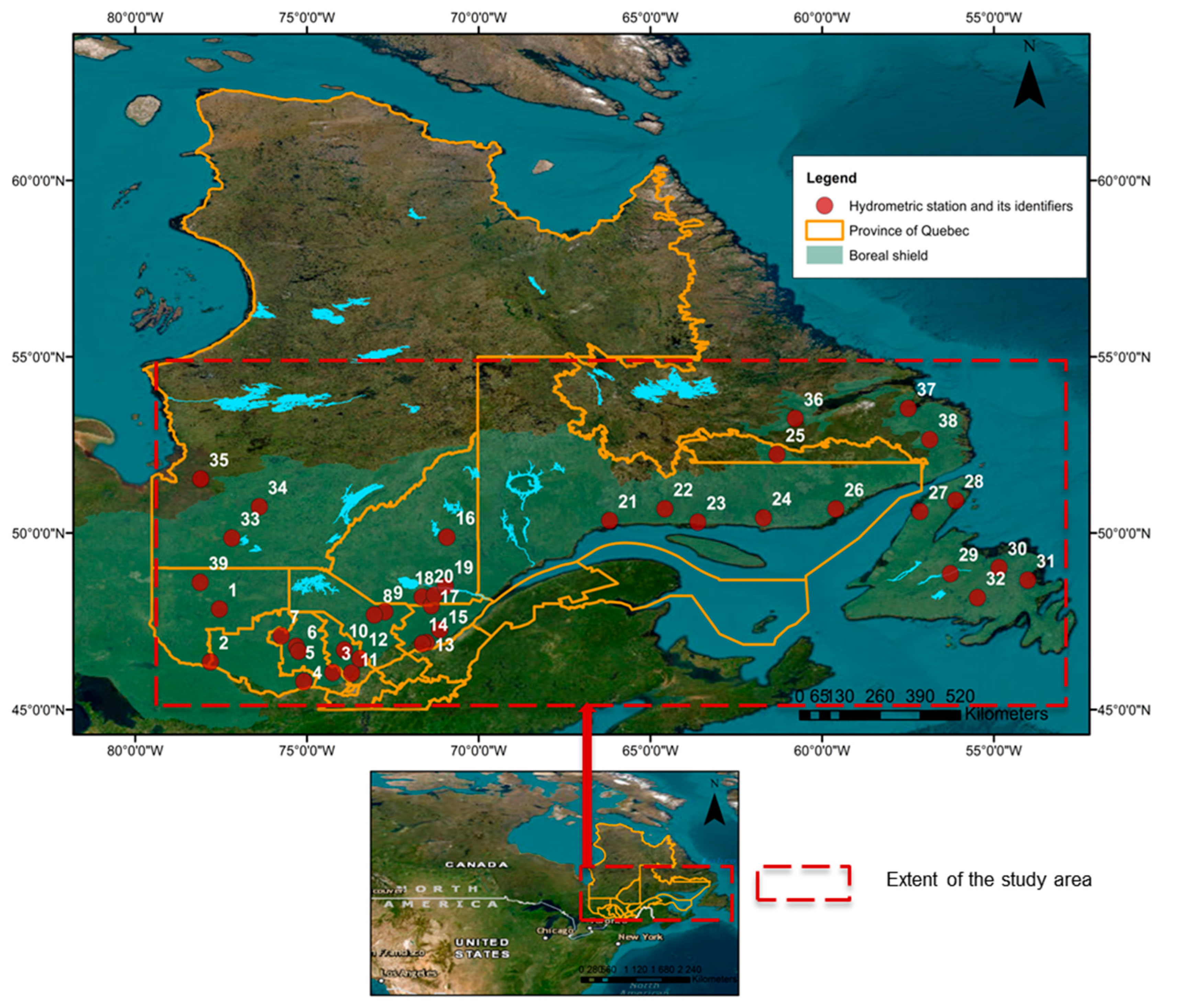
Figure 1. Overview of the study area.
Remotesensing 16 01808 g001
Figure 2. Radar image coverage across the study area.
Remotesensing 16 01808 g002
Figure 3. HAND computation workflow (inspired from [65]).
Remotesensing 16 01808 g003
Figure 4. General flowchart of the river flow estimation approach.
Remotesensing 16 01808 g004
Figure 5. Clipping data.
Remotesensing 16 01808 g005
Figure 6. Data augmentation.
Remotesensing 16 01808 g006
Figure 7. An overview of the convolutional neural network (CNN) architecture.
Remotesensing 16 01808 g007
Figure 8. An illustration of the effect of adding HAND on the accuracy of river flow estimation. (a) Flow estimation using only SAR data and (b) flow estimation using SAR data plus HAND.
Remotesensing 16 01808 g008
Figure 9. Illustration of some examples of overestimated or underestimated flow predictions.
Remotesensing 16 01808 g009
Figure 10. Flow prediction using data that are obtained within a two-km buffer around the hydrometric station.
Remotesensing 16 01808 g010
Figure 11. Flow estimation using data passing through the hydrometric station.
Remotesensing 16 01808 g011
Figure 12. Occurrence of NSE in the 15 hydrometric stations.
Remotesensing 16 01808 g012
Figure 13. Analysis of station-by-station flow estimation on different dates and under different flow conditions. River flow varies from 33 to 650 m3/s.
Remotesensing 16 01808 g013
Figure 14. Analysis of station-by-station flow estimation on different dates and under different flow conditions. River flow varies from 12 to 22 m3/s.
Remotesensing 16 01808 g014
Table 1. Descriptive statistics of hydrometric stations that were used for river flow estimation.
Range of Values
at the Stations
Width of River at Station (in m)Catchment Area (km2)Instantaneous
River Flow
m3/s
Minimum16.099.00.1
Mean112.07456.080.0
Maximum431.092,500.0750.0
Standard deviation (SD)105.015,497.0120.0
Disclaimer/Publisher’s Note: The statements, opinions and data contained in all publications are solely those of the individual author(s) and contributor(s) and not of MDPI and/or the editor(s). MDPI and/or the editor(s) disclaim responsibility for any injury to people or property resulting from any ideas, methods, instructions or products referred to in the content.