A Geometry-Compensated Sensitivity Study of Polarimetric Bistatic Scattering for Rough Surface Observation

Abstract

The use of bistatic polarimetric SAR for rough surface observation has attracted increasing interest in recent years, with its acquisition of additional polarimetric information. In this paper, we investigate the sensitivity of polarimetric variables to soil moisture and surface roughness, with the intention of locating favorable bistatic geometries for soil moisture retrieval. However, in the bistatic setting, the expanded imaging geometry is convolved with the polarimetric scattering response along with the in-scene variations in the soil moisture and surface roughness. The probing polarization states continuously evolve with the bistatic geometry, incurring varying polarization orientation angles. In this investigation, we propose to first compensate the bistatic polarimetric observations for the geometry-induced polarization rotation. Simulations based on a two-scale rough surface scattering model are then used to evaluate the optimal imaging geometry for the best sensitivity to the soil moisture content. We show the different sensing geometries associated with a full list of common polarimetric variables, as we seek favorable bistatic geometries in non-specular directions. The influences of both surface roughness scales are evaluated, with the small-scale roughness parameter imposing the greatest limitation on our results.

1. Introduction

Bistatic synthetic aperture radar (SAR) offers an attractive imaging mode by removing the geometric restrictions of monostatic imaging. On the other hand, it also introduces an extra, important design parameter to the planning of data collections. Amid various bistatic geometries, we desire a bistatic configuration that can improve the sensing utility to the greatest extent. In this paper, we focus on rough surface sensing with the goal of enhancing soil moisture measurements.

It is well known that soil moisture-related permittivity and surface roughness have a comparable influence on the scattering response from rough surfaces. A favorable configuration arises when the sensitivity to the soil moisture content (SMC) increases, while the impact from roughness is relatively small. According to earlier sensitivity studies, SAR intensities acquired near the forward specular direction are better suited than the backscatter observations for SMC estimation by virtue of a reduced dependence on surface roughness [1,2,3]. GPS reflectance data show a strong correlation between specular radar returns and field SMC measurements [4]. However, the spatial resolution becomes much poorer in the specular geometry [5].

A polarimetric system collects rich scattering information using multiple polarization channels. It is generally held that the roughness factor in radar scattering can be mitigated using polarimetric radar variables. This premise is particularly evident from the small perturbation method (SPM) theory, in which the surface roughness separates as a common scaling factor from the polarimetric observations [6,7]. With its simple analytical solution, the SPM provides the foundation for the improvement of SMC estimation from multi-polarization radar data [8,9]. However, it is only applicable to slightly rough surfaces where the surface height variation is small with respect to the incidence wavelength. We note that, even at lower frequencies (such as the L-band), the typical roughness in a natural environment exceeds the valid SPM region [10].

As the surface roughness increases, the factors of permittivity and roughness become significantly coupled in the scattered response [11]. Therefore, we cannot neglect the roughness factor in the scattering from most natural surfaces. Nevertheless, simulations based on the advanced integral equation model (AIEM), which is capable of predicting surface scattering data over a wide range of roughness conditions [12,13], still show promise as the intensity ratio between HH and VV, or between HH-VV and HH+VV, has improved sensitivity to SMC [2,3]. Nonetheless, the optimal geometry is still located near the specular direction.

We note that with a full polarimetric SAR (PolSAR), many combinations of the polarization channels are available. In addition, when equipped with full polarimetric capabilities, a bistatic system collects additional scattering information with more degrees of freedom than that of monostatic PolSAR observations. Accordingly, the use of bistatic PolSAR may present a potential advantage in the inference of physical scatter properties. Our main objective is to investigate which polarimetric variables show heightened sensitivity to soil moisture while suppressing the roughness factor. In particular, we explore the possible set of polarimetric variables that can perform well for bistatic geometries away from the specular direction.

The choice of polarimetric combinations should also be physically meaningful. This is a major challenge because, in a general bistatic setting, all the polarization channels are entangled with the specific bistatic geometry [14]. In particular, H-pol (or V-pol) in the transmitter and its counterpart in the receiver are not always aligned in the same direction. In fact, their difference will continuously evolve with different bistatic geometries. Then, for example, the reference channel labels ‘HH’ and ‘VV’ do not necessarily imply the special characteristics of co-polarization.

Choosing a proper polarimetric reference frame mitigates effects due to the bistatic geometry. Firstly, we rotate the polarization orientation to reduce the geometry-induced difference, which is equivalent to using a different reference system [15]. Following along this vein, as the analysis standard, we adopt a reference system constructed using the bistatic plane, the one formed by the incidence and scattering wave vectors. A common horizontal polarization is defined as the linear polarization orthogonal to the bistatic plane; the vertical polarization differs between incidence and scattering but is contained inside the bistatic plane. With this reference frame, we obtain geometry-compensated polarization channels that can be transformed from the native polarization bases.

Secondly, we also wish to evaluate the polarimetric variables that are independent of the polarization bases. A changing bistatic geometry results in a variation in the scattering mechanisms but also a variation in the polarization orientation angles (POA). By explicitly separating the polarization orientation factors, we hope to retain the intrinsic, characteristic scattering parameters associated with the physical scattering process. This will be accomplished by utilizing singular value decomposition (SVD) on the bistatic scattering matrices of individual coherent scattering components.

To facilitate the polarization basis transformation, we adopt the two-scale rough surface scattering model (TSM) in the simulation. The TSM was developed as an extension to the SPM such that we can overcome the SPM’s limited validity for rougher surfaces [16,17]. The TSM assumes that the surface roughness comprises two separate variation regimes: a small-scale regime varying horizontally on the order of the wavelength and vertically much smaller than a wavelength, which satisfies the SPM; and a large-scale regime varying horizontally on scales much larger than a wavelength and vertically on the order of the wavelength or higher, which accounts for random surface orientations and POA variation [10]. Then, the TSM accommodates the increased surface roughness through an ensemble of randomly oriented surface facets. Locally, on each facet, the small-scale variation applies. Because the roughness scales are defined in terms of the wavelength, as we will discuss later, the practical TSM range is still limited to low-frequency bands. While the empirical roughness division makes it rather difficult to rigorously validate against numerically simulated data, indirect validation has demonstrated good agreement between TSM-derived estimates from backscatter data and field measurements, even in selected cases at the X-band [16]. In contrast, AIEM has a wide applicable range with extensive validation. Nevertheless, the TSM offers an attractive option by explicitly revealing the roughness effect through POA variation, and there are established polarimetric techniques to evaluate POA from PolSAR imagery [8,9,10].

This paper is organized as follows. The TSM is described in Section 2 and the sensitivity evaluation approach is described in Section 3. In Section 4, we show selected results for a horizontal rough surface under a fixed incidence beam at various reception directions. Discussions and conclusions are provided in Section 5.

2. The Two-Scale Rough Surface Scattering Model

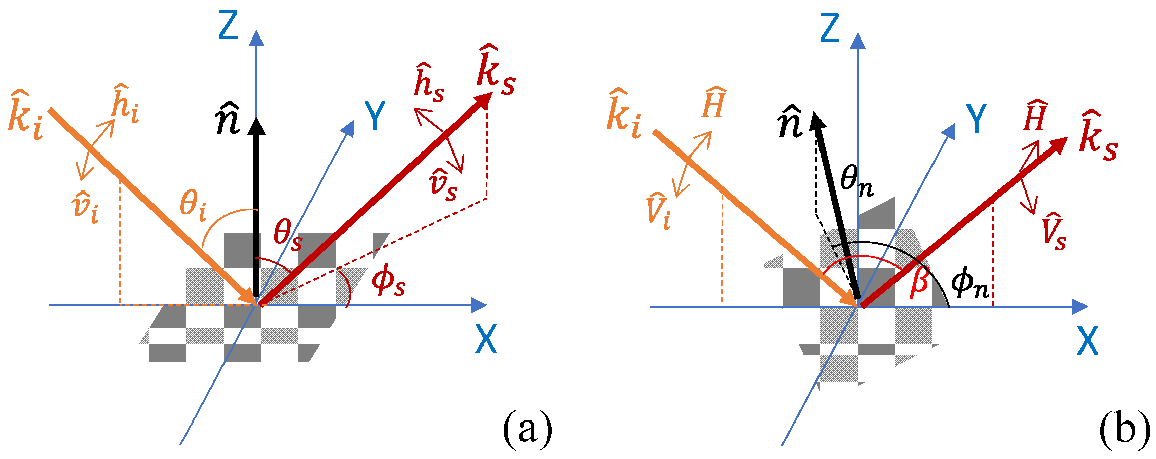
Figure 1a shows a general bistatic sensing geometry and its native polarization bases. The incoming beam is fixed at the incidence angle ${\theta }_i$ from the $-X$ direction and the scattered wave is received at the direction with zenith angle ${\theta }_s$ and azimuth angle ${\varphi }_s.$ The subscripts ‘i’ and ‘s’ are used to delineate the incidence wave and the scattered wave, respectively. The backscattering direction features ${\varphi }_s=\pi$ and the forward scattering direction features ${\varphi }_s=0$. The native probing polarizations used in the bistatic system are defined with respect to the $Z$ direction, such that ${\widehat{h}}_{i,s}=\widehat{Z}\times {\widehat{k}}_{i,s}/\sin {\theta }_{i,s}$ and ${\widehat{v}}_{i,s}={\widehat{h}}_{i,s}\times {\widehat{k}}_{i,s}$.

Under this bistatic geometry, for a horizontal surface (with its normal vector $\widehat{n}=\widehat{Z}$), the polarimetric scattering response can be expressed as [18]

$$s_{pq}\left({\epsilon }_r;{\theta }_i,{\theta }_s,{\varphi }_s\right)=k_0^2\cos {\theta }_i\cos {\theta }_s{W}^{\frac{1}{2}}\left({\overline{k}}_{\rho s}-{\overline{k}}_{\rho i}\right)\left(1-{\epsilon }_r\right)g_{pq}\left({\epsilon }_r;{\theta }_i,{\theta }_s,{\varphi }_s\right),$$

(1)

where subscripts $p$ and $q$, respectively, denote the receiving polarization and the illuminating polarization; $k_0$ is the wavenumber; $W$ is the surface roughness spectrum; ${\overline{k}}_{\rho }$ is the horizontal component of the wave vectors; and ${\epsilon }_r$ stands for the relative permittivity. The SPM kernel function $g_{pq}$ expresses all of the polarization-dependent terms; for linearly polarized H/V waves, they can be written as follows [19]:

$$g_{hh}=\frac{\cos {\varphi }_s}{\left(\cos {\theta }_i+\sqrt{{\epsilon }_r-{\sin }^2{\theta }_i}\right)\left(\cos {\theta }_s+\sqrt{{\epsilon }_r-{\sin }^2{\theta }_s}\right)},$$

(2)

$$g_{hv}=\frac{\sin {\varphi }_s\sqrt{{\epsilon }_r-{\sin }^2{\theta }_i}}{\left({\epsilon }_r\cos {\theta }_i+\sqrt{{\epsilon }_r-{\sin }^2{\theta }_i}\right)\left(\cos {\theta }_s+\sqrt{{\epsilon }_r-{\sin }^2{\theta }_s}\right)},$$

(3)

$$g_{vh}=\frac{\sin {\varphi }_s\sqrt{{\epsilon }_r-{\sin }^2{\theta }_s}}{\left(\cos {\theta }_i+\sqrt{{\epsilon }_r-{\sin }^2{\theta }_i}\right)\left({\epsilon }_r\cos {\theta }_s+\sqrt{{\epsilon }_r-{\sin }^2{\theta }_s}\right)},$$

(4)

$$g_{vv}=\frac{{\epsilon }_r\sin {\theta }_i\sin {\theta }_s-\cos {\varphi }_s\sqrt{{\epsilon }_r-{\sin }^2{\theta }_i}\sqrt{{\epsilon }_r-{\sin }^2{\theta }_s}}{\left({\epsilon }_r\cos {\theta }_i+\sqrt{{\epsilon }_r-{\sin }^2{\theta }_i}\right)\left({\epsilon }_r\cos {\theta }_s+\sqrt{{\epsilon }_r-{\sin }^2{\theta }_s}\right)}.$$

(5)

Note that, for compactness, the subscript tags ‘i’ and ‘s’ are dropped on the polarization states; in other words, the polarization symbol $h$ (or $v$) at the two subscript positions implicitly represents different polarizations between the incidence side and the scattering side.

The surface can be oriented in different directions either due to increased roughness or due to terrain slopes. When $\widehat{n}\ne \widehat{Z}$, the surface orientation affects the polarimetric scattering response in two ways: by altering the local beam angles and by inducing polarization rotations.

The beam angles in Equations (1)–(5) need to be replaced with the following local angles, such as

$${\tilde{\theta }}_i={\cos }^{-1}\left(-{\widehat{k}}_i\cdot \widehat{n}\right),$$

(6)

$${\tilde{\theta }}_s={\cos }^{-1}\left({\widehat{k}}_s\cdot \widehat{n}\right),$$

(7)

$${\tilde{\varphi }}_s={\cos }^{-1}\left[(\cos {\tilde{\theta }}_i\cos {\tilde{\theta }}_s+{\widehat{k}}_i\cdot {\widehat{k}}_s)/\left(\sin {\tilde{\theta }}_i\sin {\tilde{\theta }}_s\right)\right].$$

(8)

The horizontal wave vector components shall also be updated accordingly through

$${\overline{k}}_{\rho s}-{\overline{k}}_{\rho i}=k_0\cdot \left[{\widehat{k}}_s-{\widehat{k}}_i-\left(\cos {\tilde{\theta }}_i+\cos {\tilde{\theta }}_s\right)\widehat{n}\right].$$

(9)

Substituting Equations (6)–(9) in Equations (1)–(5) produces the generic rough surface scattering matrix in the local reference system, $\tilde{\mathbf{S}}=\left[{\tilde{s}}_{pq}\left({\epsilon }_r;{\tilde{\theta }}_i,{\tilde{\theta }}_s,{\tilde{\varphi }}_s\right)\right]$.

In this local system, the polarizations are redefined with respect to the surface normal vector $\widehat{n}$ such that, for example, ${\tilde{h}}_{i,s}=\widehat{n}\times {\widehat{k}}_{i,s}/\sin {\tilde{\theta }}_{i,s}$. Because the probing polarizations used in the observation are different from those defined in the local system, a polarization basis rotation ensues to transform the generic rough surface scattering matrix $\tilde{\mathbf{S}}$ into the observed scattering matrix $\mathbf{S}$ through

$$\mathbf{S}=\left[\begin{array}{cc}\cos {\alpha }_s& -\sin {\alpha }_s\\ \sin {\alpha }_s& \cos {\alpha }_s\end{array}\right]\tilde{\mathbf{S}}\left[\begin{array}{cc}\cos {\alpha }_i& \sin {\alpha }_i\\ -\sin {\alpha }_i& \cos {\alpha }_i\end{array}\right],$$

(10)

where $\tan {\alpha }_i={\widehat{v}}_i\cdot {\tilde{h}}_i/{\widehat{h}}_i\cdot {\tilde{h}}_i$ and $\tan {\alpha }_s={\widehat{v}}_s\cdot {\tilde{h}}_s/{\widehat{h}}_s\cdot {\tilde{h}}_s$. Let ${\theta }_n$ and ${\varphi }_n$ stand for the orientation angle of the surface normal vector. It is straightforward to derive the polarization rotation angles as

$${\alpha }_i={\tan }^{-1}\left(\frac{\sin {\theta }_n\sin {\varphi }_n}{\cos {\theta }_n\sin {\theta }_i+\sin {\theta }_n\cos {\varphi }_n\cos {\theta }_i}\right),$$

(11)

$${\alpha }_s={\tan }^{-1}\left[\frac{\sin {\theta }_n\sin \left({\varphi }_n-{\varphi }_s\right)}{\cos {\theta }_n\sin {\theta }_s-\sin {\theta }_n\cos \left({\varphi }_n-{\varphi }_s\right)\cos {\theta }_s}\right].$$

(12)

We assume that the mean surface orientation associated with sloped terrain is known. Its determination—for example, from DEM data—is beyond the scope of this work. In this case, ${\theta }_n$ and ${\varphi }_n$ are deterministic variables, and, using the polarization rotation matrices, we can convert the measurement effectively to the case of a horizontal rough surface. Hence, without loss of generality, we will limit our study to the horizontal surface geometry.

Now, all that remains is the random surface orientation variation induced by roughness. Although, overall, the elementary facets have a vertical mean orientation, individually, each features a non-vertical normal vector. In this case, ${\theta }_n$ and ${\varphi }_n$ are random variables and their variation increases as the terrain surface becomes rougher. Then, Equations (10)–(12) relate the roughness factor to POA modulation. The TSM formulation addresses the limited validation range of the SPM formulation by incorporating random orientation modulation into the polarimetric scattering response. This modulation is assumed to be derived from the large-scale roughness regime, whereas the SPM scattering mechanism is derived from the small-scale roughness regime associated with the roughness spectrum $W$. The latter is commonly taken to be isotropically distributed according to a Gaussian or exponential correlation function. For the large-scale roughness, we introduce a distribution for facet slopes or a distribution directly for orientation angles.

In [16], a joint Gaussian distribution was chosen to describe the surface slope variation associated with the large-scale roughness. We noticed that the slope distribution tended to deviate from Gaussian if the variation was very high. In this work, we opt to use the von Mises–Fisher (vMF) distribution to describe the surface orientation variation. The vMF distribution describes a unimodal directional distribution with cyclic angular variables [20]. Specifically, in terms of ${\theta }_n$ and ${\varphi }_n$ with zero mean, the random orientation follows

$$f\left({\theta }_n,{\varphi }_n;\kappa \right)=C{e}^{\kappa \cos {\theta }_n},0\le {\theta }_n\le \pi /2,$$

(13)

where $\kappa$ is a concentration parameter that controls the spread of the distribution, with a large value denoting a narrow distribution, and $C$ is a normalization constant. We note that

$$C=\frac{\kappa \exp \left(-k/2\right)}{4\pi \sinh \left(\kappa /2\right)}$$

(14)

for the domain specified in Equation (13).

Finally, we incoherently integrate over the random, polarimetrically rotated scattering vectors to form the second-order bistatic polarimetric dataset. In practice, the scattering from rough surfaces is a statistical process, subject to strong speckle variation. The speckle will manifest in the dataset if we simulate an ensemble of oriented facet realizations and consider their incoherent summation. In this study, we wish to explore the theoretical geometry-dependent sensitivity relations. Hence, we do not consider the speckle effect; instead, we only use numerical integration to compute all of the polarimetric covariance matrix elements following

$$〈s_{pq}{s}_{uv}^{*}〉=\iint s_{pq}\left({\theta }_n,{\varphi }_n;{\epsilon }_r\right)s_{uv}^{*}\left({\theta }_n,{\varphi }_n;{\epsilon }_r\right)f\left({\theta }_n,{\varphi }_n;\kappa \right)\sin {\theta }_n{1}_n\left({\theta }_n,{\varphi }_n\right)d{\theta }_{n}d{\varphi }_n,$$

(15)

where $1_n$ is an indicator function defined as

$$1_n\left(\theta ,\varphi \right)=\left\{\begin{array}{cc}1& \left(\theta ,\varphi \right)\in \left\{{\theta }_n,{\varphi }_n|0\le {\tilde{\theta }}_i<\frac{\pi }{2},0\le {\tilde{\theta }}_s<\frac{\pi }{2}\right\}\\ 0& otherwise.\end{array}\right.,$$

(16)

3. The Sensitivity Evaluation Scheme

3.1. The Geometry-Compensated Reference System

It is of fundamental interest to evaluate how the different polarimetric variables respond to soil moisture and surface roughness. In the framework of bistatic scattering, we obtain four independent polarization channels, from which numerous combinations can be formed. A list of ratios and correlation terms can be defined straightforwardly over these polarization channels (see

Table 1. The list of direct polarimetric variables.

$⟨{\left|HH\right|}^2⟩$	$⟨{\left|VH\right|}^2⟩/⟨{\left|HH\right|}^2⟩$ ${\rho }_{VHHH}$	$⟨{\left|HV\right|}^2⟩/⟨{\left|HH\right|}^2⟩$ ${\rho }_{HVHH}$	$⟨{\left|VV\right|}^2⟩/⟨{\left|HH\right|}^2⟩$ ${\rho }_{VVHH}$
-	$⟨{\left|VH\right|}^2⟩$	$⟨{\left|VH\right|}^2⟩/⟨{\left|HV\right|}^2⟩$ ${\rho }_{VHHV}$	$⟨{\left|VH\right|}^2⟩/⟨{\left|VV\right|}^2⟩$ ${\rho }_{VHVV}$
-	-	$⟨{\left|HV\right|}^2⟩$	$⟨{\left|HV\right|}^2⟩/⟨{\left|VV\right|}^2⟩$ ${\rho }_{HVVV}$
-	-	-	$⟨{\left|VV\right|}^2⟩$

) or over a variety of their linear combinations. However, we need to ensure that they are physically meaningful.

Co-polarization and cross-polarization are clearly defined in the monostatic scenario. However, a systematic polarization difference is always contained in the bistatic scenario. As demonstrated in Figure 1a, ${\widehat{v}}_s\ne {\widehat{v}}_i$, except in the backscattering direction, and ${\widehat{h}}_s$ differs from ${\widehat{h}}_i$ by an angle of ${\varphi }_s$. When ${\varphi }_s=\pm {90}^{\circ }$, ${\widehat{h}}_s$ and ${\widehat{h}}_i$ are in fact orthogonal. 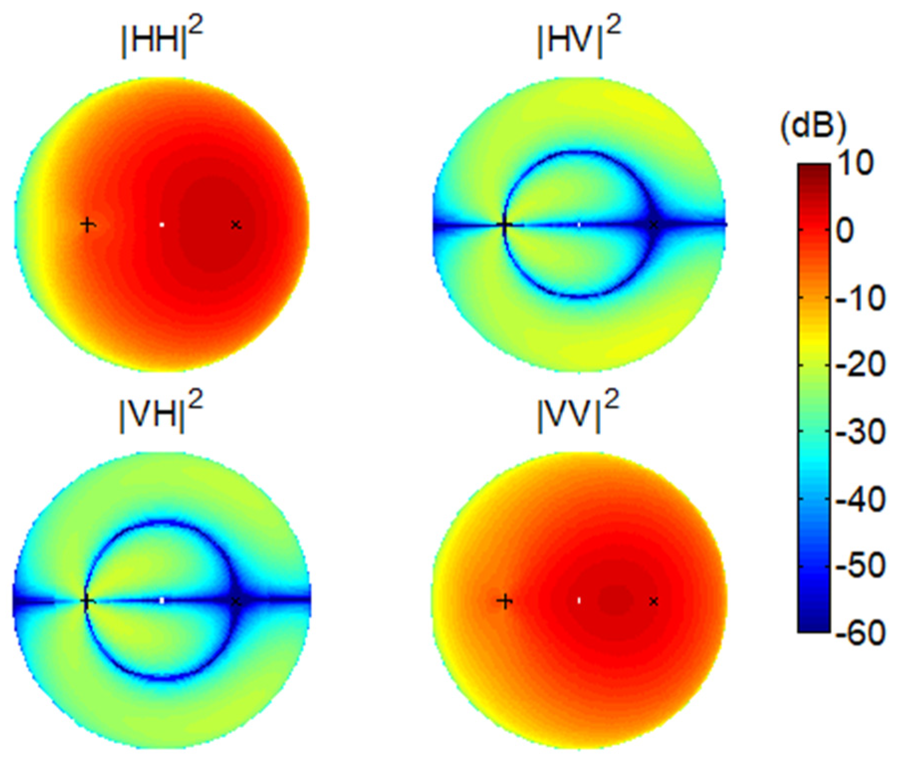Figure 2 shows a typical set of bistatic scattering intensities from a horizontal surface in the four polarization channels using the SPM. We fix the incidence direction but vary the scattering direction (${\theta }_s,{\varphi }_s$) in the full upper hemisphere (also refer to [21] for the detailed simulation settings). We can see that the HH channel reaches minima in the cross-plane of the incidence where both the VH and HV channels are strong. Coincidently, the two horizontal states in the transmitter and the receiver are orthogonal.

Furthermore, this polarization difference may have other significant consequences. In monostatic polarimetry, the co-polarization combination HH+VV is advantageous due to being independent of the POA variation; in bistatic polarimetry, it loses this appealing property.

In order to minimize the impact of the geometry-induced polarization difference, we use an alternative polarization reference system, as shown in Figure 1b. This frame is centered on the bistatic plane, with a common horizontal polarization defined as orthogonal to the bistatic plane and the vertical polarization defined accordingly inside the bistatic plane. The polarizations are expressed as

$$\widehat{H}={\widehat{k}}_s\times {\widehat{k}}_i/\sin \beta ,$$

(17)

$${\widehat{V}}_i=\widehat{H}\times {\widehat{k}}_i,$$

(18)

$${\widehat{V}}_s=\widehat{H}\times {\widehat{k}}_s,$$

(19)

where $\beta$ stands for the bistatic angle. This reference frame has been used before. We can further set the bisector line between $-{\widehat{k}}_i$ and ${\widehat{k}}_s$ as the new zenith direction. Its adoption in our sensitivity evaluation is highlighted with the following merits: a common $\widehat{H}$ shared by both the incidence and scattered waves, the orthogonality between $\widehat{H}$ and ${\widehat{V}}_{i,s}$, and the established relation ${\widehat{V}}_i\cdot {\widehat{V}}_s=-\cos \beta$. In some sense, we mitigate the geometry dependence to the utmost degree and reestablish the cross-polarization channels for polarimetric scattering analysis.

The transformation between the native polarization system and the new reference system is readily attained by applying the following polarization rotation operation:

$${\mathbf{S}}_{\left\{H,V\right\}}=\left[\begin{array}{cc}\widehat{H}\cdot {\widehat{h}}_s& \widehat{H}\cdot {\widehat{v}}_s\\ {\widehat{V}}_s\cdot {\widehat{h}}_s& {\widehat{V}}_s\cdot {\widehat{v}}_s\end{array}\right]{\mathbf{S}}_{\left\{\mathit{h},\mathit{v}\right\}}\left[\begin{array}{cc}{\widehat{h}}_i\cdot \widehat{H}& {\widehat{h}}_i\cdot {\widehat{V}}_i\\ {\widehat{v}}_i\cdot \widehat{H}& {\widehat{v}}_i\cdot {\widehat{V}}_i\end{array}\right].$$

(20)

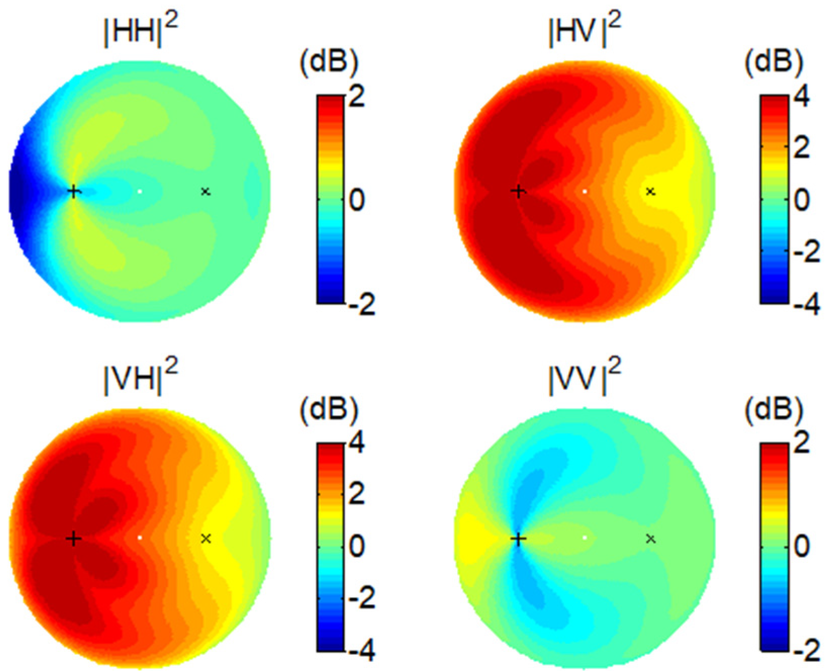
In the rest of this paper, we only use ${\mathbf{S}}_{\left\{H,V\right\}}$; therefore, the subscript will be dropped. The same intensities shown in Figure 2 are reproduced in the standard reference system in Figure 3. We see that both the HV and the VH channels now have lower intensities and the discontinuity in the HH and VV channels largely disappears.

3.2. The Characteristic Polarimetric Variables

The fact that polarimetric observations of the same scattering process vary with the polarization basis can be a nuisance. Considering this, we prefer to use the characteristic polarimetric variables that are tied more to the intrinsic scattering process.

In order to derive the characteristic variables, we diagonalize the bistatic scattering matrix using singular value decomposition (SVD), such that

$$\mathbf{S}=\mathbf{U}\mathbf{D}{\mathbf{V}}^H=\mathbf{U}\left[\begin{array}{cc}{s}_a& 0\\ 0& s_b\end{array}\right]{\mathbf{V}}^H,$$

(21)

where the superscript ‘H’ denotes a conjugate transpose, and $s_a$ and $s_b$ present a pair of characteristic scattering coefficients. Both $\mathbf{U}$ and $\mathbf{V}$ are unitary matrices representing polarization basis transformations from the observation bases to the characteristic bases, which are defined as a product of the polarization rotation factor and ellipticity factor, such that

$$\mathbf{U}=\left[\begin{array}{cc}\cos {\tau }_s& -\sin {\tau }_s\\ \sin {\tau }_s& \cos {\tau }_s\end{array}\right]\left[\begin{array}{cc}\cos {ϵ}_s& j\sin {ϵ}_s\\ j\sin {ϵ}_s& \cos {ϵ}_s\end{array}\right],$$

(22)

$$\mathbf{V}=\left[\begin{array}{cc}\cos {\tau }_i& -\sin {\tau }_i\\ \sin {\tau }_i& \cos {\tau }_i\end{array}\right]\left[\begin{array}{cc}\cos {ϵ}_i& j\sin {ϵ}_i\\ j\sin {ϵ}_i& \cos {ϵ}_i\end{array}\right].$$

(23)

Angles $\tau$ and $ϵ$ represent the orientation and ellipticity of the characteristic polarization state [22]. The former is closely related to both the system polarization basis and the sensing geometry; the adopted reference standard helps us to establish a useful baseline for its interpretation. The latter measures the helicity and symmetry in the scattering process.

The specific forms of $\mathbf{U}$ and $\mathbf{V}$ above impose a constraint on the unitary transformation, so that $s_a$ and $s_b$ remain as complex-valued terms. We define their scattering ratio and phase difference to represent the intrinsic, characteristic scattering properties:

$$\mathsf{\Gamma }={\left|s_a\right|}^2/{\left|s_b\right|}^2,$$

(24)

$$\psi =\angle s_a{s}_b^{*}.$$

(25)

However, the polarimetric scattering response presents an incoherent process due to the surface roughness. This requires an expression of the covariance matrix to completely capture the scattering information, through

$$\mathsf{\Sigma }=〈\underset{\_}{\mathit{S}}{\underset{\_}{\mathit{S}}}^H〉,\underset{\_}{\mathit{S}}={\left[s_{HH}{s}_{VH}{s}_{HV}{s}_{VV}\right]}^T.$$

(26)

This covariance matrix can be decomposed into four uncorrelated scattering components in terms of its eigenvectors, namely

$$\mathsf{\Sigma }={\sum }_{i=1}^4{p}_i{\underset{\_}{\mathit{S}}}_i{\underset{\_}{\mathit{S}}}_i^H.$$

(27)

Then, each of the eigen-scattering components can be diagonalized using Equation (21) to extract the characteristic polarization states, as well as the characteristic scattering properties.

Table 2. The list of characteristic polarimetric variables.

$p_1$ ${\tau }_{1i,s},{ϵ}_{1i,s},{\mathsf{\Gamma }}_1,{\psi }_1$	$p_2/p_1$	$p_3/p_1$	$p_4/p_1$
-	$p_2$ ${\tau }_{2i,s},{ϵ}_{2i,s},{\mathsf{\Gamma }}_2,{\psi }_2$	$p_3/p_2$	$p_4/p_2$
-	-	$p_3$ ${\tau }_{3i,s},{ϵ}_{3i,s},{\mathsf{\Gamma }}_3,{\psi }_3$	$p_4/p_3$
-	-	-	$p_4$ ${\tau }_{4i,s},{ϵ}_{4i,s},{\mathsf{\Gamma }}_4,{\psi }_4$

lists all of the characteristic polarimetric variables. In particular, the sets $\left\{p\right\}$, {$\mathsf{\Gamma }$}, and {$\psi$}c are all independent of the polarization basis.

3.3. The Sensitivity Metrics

The dependence of the surface scattering on the soil moisture is generated by the complex permittivity of the soil medium. For convenience, we use the volumetric SMC in the evaluation. In the TSM framework, the dependence on the surface roughness involves multiple factors, including the specific roughness spectrum and its parameters, as well as the large-scale roughness variation. Because we specifically associate the large-scale portion of the surface roughness with the surface orientation variation, for the small-scale roughness, we simply adopt the Gaussian spectrum model. The Gaussian roughness spectrum is expressed as

$$W\left(k\right)=\frac{1}{2}{L}^2\exp \left(-\frac{L^2{k}^2}{4}\right),$$

(28)

where $L$ is the correlation length. The root mean square (rms) height is omitted in the above spectrum because it is irrelevant to polarimetric variables. For the large-scale roughness, we use the vMF distribution and $\kappa$ is the variation parameter.

The scattering response is highly nonlinear. Complete characterization requires an evaluation of its slope with various combinations of moisture and roughness parameters. To make the evaluation tractable, we use averages or approximations at several selected baseline settings.

In [2], a quality factor was adopted to measure the balance between the moisture effect and the roughness effect on the bistatic observations. For a variable $x$, the quality factor is defined as

$$I\left(x\right)=\frac{\Delta x/\Delta sm}{\Delta x/\Delta sm+\Delta x/\Delta rough},$$

(29)

where $\Delta x/\Delta sm$ stands for the change rate on $x$ as incurred by the difference in soil moisture and $\Delta x/\Delta rough$ for that as incurred by the difference in surface roughness. However, they have different units and their values would vary with the type of parameters used.

Instead, we use a set of baseline parameters, as listed in

Table 3. The comparison of the baseline settings of the rough surface parameters.

	SMC	$\mathit{L}$	$\mathit{\kappa }$
Baseline Low	15%	$0.5\lambda$	50
Baseline High	25%	$0.1\lambda$	30

, between the low end, for which the moisture and the roughness are low, and the high end, for which the moisture and the roughness are high. The SMC settings at 15% and 25% apply for wet soil content away from both the dry condition and the saturated condition. The typical field range for SMC is between 5% and 35%, depending on the soil types and textures. The correlation length $L$ is set to ensure that the SPM is locally applicable at an individual surface facet. This parameter is scaled relative to the wavelength, with $k_{0}L$ varying between 0.63 and 3.14. Approximately, $L$ shall be 4.7 times greater than the rms height. A very short correlation length is not meaningful in a practical setting, whereas a very large correlation length will shift the scattering to the physical optics domain. The settings on $\kappa$ represent the spread of the random facet orientation over an ensemble of surface facets. The orientation randomness is not commonly measured in field surveys. According to our experience with POA analysis, $\kappa =50$ corresponds to a moderately rough surface, like farm fields, whereas $\kappa =30$ corresponds to a highly rough surface, as encountered in natural terrain.

Then, we evaluate the contributing factors by comparing the incurred changes between a pair of observations made among these baseline parameters. For the SMC vs. small-scale roughness, we assess the change responding to SMC as

$$\Delta sm=\left|x_{SM2,L1}-x_{SM1,L1}\right|+\left|x_{SM2,L2}-x_{SM1,L2}\right|$$

(30)

and the change responding to the correlation length as

$$\Delta rough=\left|x_{SM1,L2}-x_{SM1,L1}\right|+\left|x_{SM2,L2}-x_{SM2,L1}\right|.$$

(31)

Consequently, we obtain a unitless quality factor from

$$I_{SM-L}\left(x\right)=\frac{\Delta sm}{\Delta sm+\Delta rough}.$$

(32)

Similarly, we can evaluate a quality factor for the SMC vs. the large-scale roughness, $I_{SM-\kappa }$, using the low-end and high-end parameters of SMC and $\kappa$.

4. Case Studies and Results

For the evaluation, we run a TSM-based simulation at different soil moisture and surface roughness levels. By comparing the relative changes among the polarimetric channels, we infer the most beneficial choices of both the bistatic geometry and polarimetric variables. To estimate the soil moisture, we would prefer those reception directions at which the scattering response is more sensitive to the soil permittivity but less affected by the surface roughness.

Recall, at the core of the TSM, the assumption that the local roughness needs to be small in individual facets, compared to the carrier wavelength $\lambda$. Although, in Table 3, the roughness parameter is defined relative to $\lambda$, such that the SPM criterion is always satisfied, realistically, we relate the simulation parameters to the lower frequencies. In the following evaluation, we assume operation at the L-band with $\lambda =0.2$ m. The resolution cell spans a few meters and comprises many surface facets, each having a size comparable to $\lambda$. Accordingly, the surface height deviation among different facets is independent, since $L<\lambda$. In other words, after the local mean slope is removed, the local roughness has a short correlation length. If the system operates at short wavelengths, restricting the local roughness under a small facet size is likely impractical. Therefore, realistically, the TSM assumptions and our correlation length settings are more applicable at the P-, L-, and S-bands. Note that these also are the common system frequencies for soil moisture applications.

To simulate the full polarimetric covariance matrix, we apply the specific ${\widehat{k}}_i$ and ${\widehat{k}}_s$ pair along with ${\epsilon }_r$, $L$, and $\kappa$ to Equation (15). The integration is evaluated over a regular grid of $({\theta }_n,{\varphi }_n)$, namely the direction angles of a random orientation distribution, with ${\theta }_n\in [0^{\circ },{90}^{\circ })$ in ${0.1}^{\circ }$ stepping and ${\varphi }_n\in [-{180}^{\circ },{180}^{\circ })$in $1^{\circ }$ stepping. The accuracy of the numerical integration is checked by ensuring that the solid angle integration over $f\left({\theta }_n,{\varphi }_n,\kappa \right)$ is equal to 1. Next, the local incidence and scattering angles are evaluated for the {${\widehat{k}}_i$, ${\widehat{k}}_s$} pair at each orientation direction using Equations (6)–(8). The cases where ${\tilde{\theta }}_i>{90}^{\circ }$ or ${\tilde{\theta }}_s>{90}^{\circ }$ are considered as shadows and the corresponding directions are discarded. In general, the pdf is also very low in these directions. The computation for the polarimetric scattering coefficients is straightforward, using Equations (2)–(5) and Equations (10)–(12). They are scaled in amplitudes accounting for roughness and finally replaced in the pdf integration. The implementation is currently performed in the MATLAB environment and the computation speed is not of concern.

In the simulation, we fix the incidence angle to 30°, which corresponds to a typical illumination geometry from a spaceborne SAR. The scattered returns are computed for different scattering directions by varying (${\theta }_s$, ${\varphi }_s$), hereinafter covering the upper hemisphere in a $1^{\circ }$ grid. To evaluate the moisture-induced changes, we compute the model predictions at SMC values of 15% (${\epsilon }_r=$ 9.2 − i0.5) and 25% (${\epsilon }_r=$ 14.6 − i0.9), whereas the roughness settings are fixed. The roughness-induced changes are evaluated in a similar manner. The high baseline listed in Table 3 is adopted as the control parameters in the comparison study. Specifically, when evaluating $I_{SM-L}$, we set $\kappa$ to 30, whereas, when evaluating $I_{SM-\kappa }$, we set $L$ to $0.1\lambda$.

4.1. Normalized Scattering Intensity

To understand the overall scattering variation but with the absolute calibration factor removed, we normalize the scattering intensities against the total scattered power.

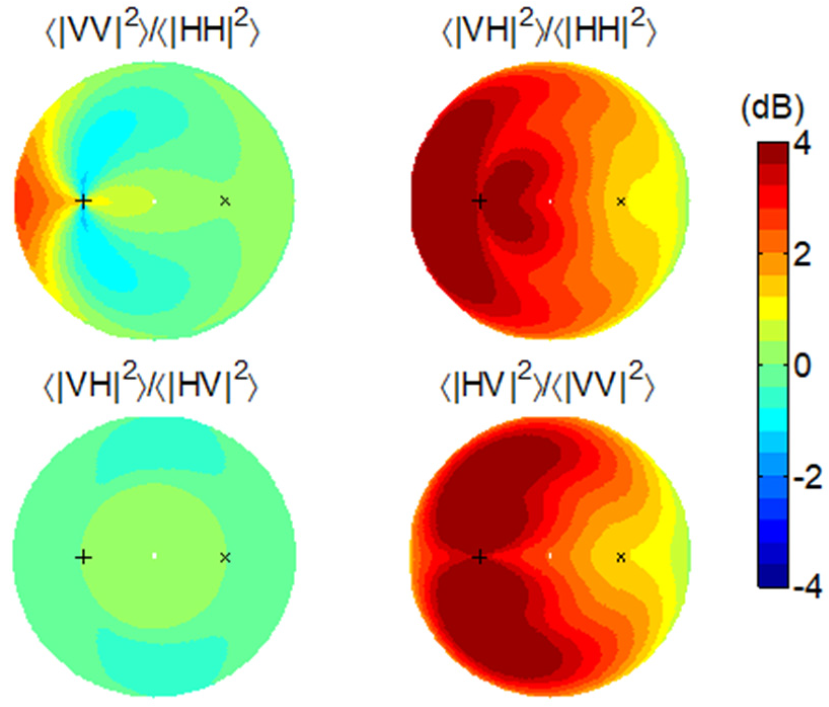
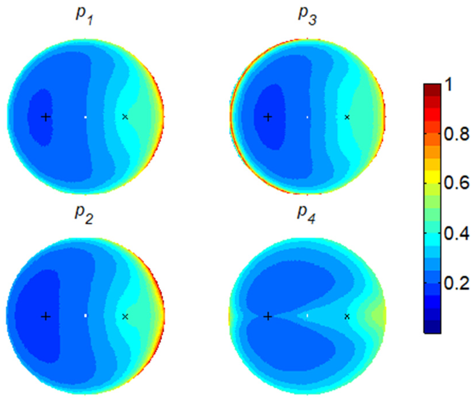
Figure 4 depicts the changes in the normalized intensities as the SMC increases from 15% to 25%. We see only a small change in HH and VV for the majority of the bistatic geometries. At the forward grazing directions, however, HH is diminished while VV is enhanced, moderately but perceptibly. Consistent increases are present on HV and VH in response to the higher SMC, indicating an enhanced cross-polarization response to the moist rough surface.

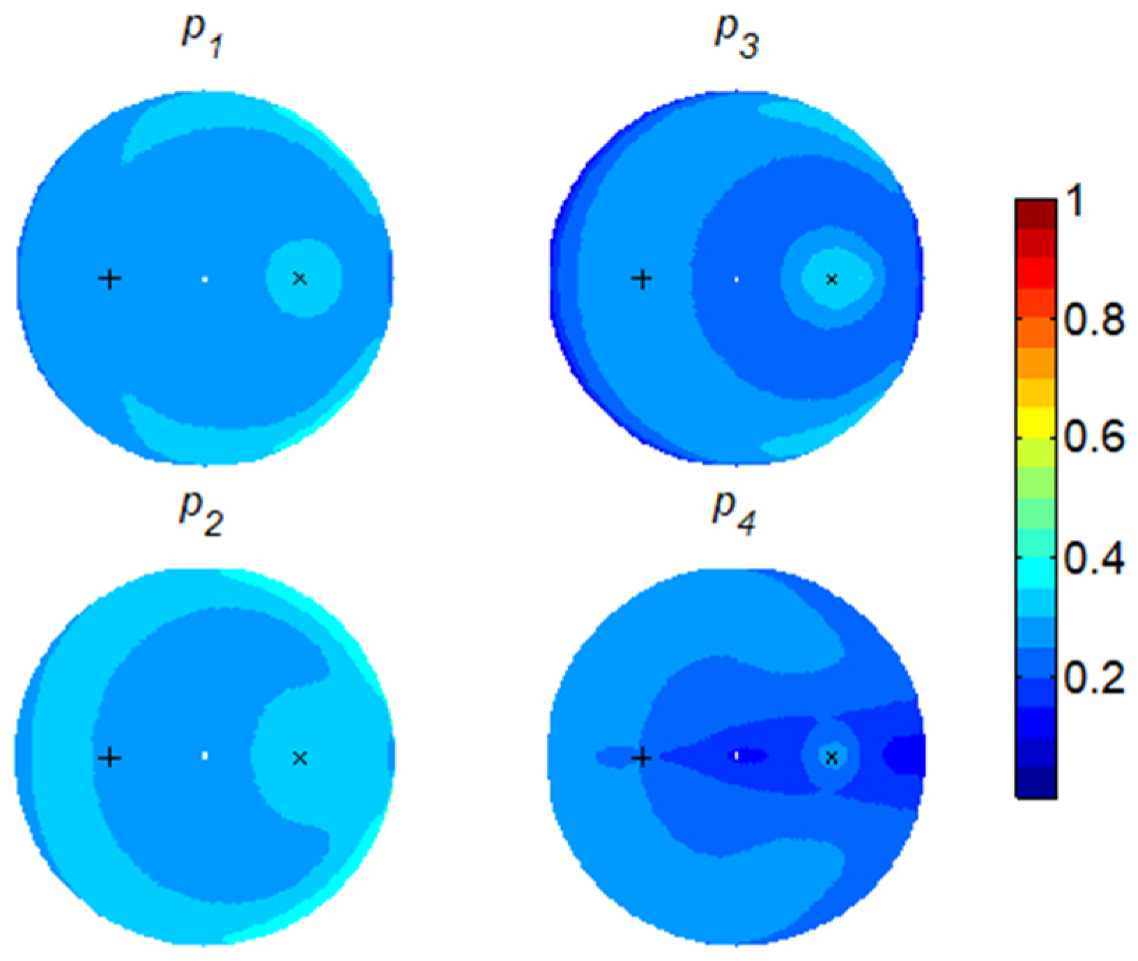
Figure 5 depicts the scattering change at 25% SMC as the small-scale roughness increases by reducing the correlation length from $0.5\lambda$ to $0.1\lambda$. Higher variations prevail in all polarimetric channels. Even though, at the core, the SPM scattering from each individual facet is independent of the small-scale roughness, collectively, due to the orientation effect from the large-scale roughness, the small-scale roughness will be reflected in the scattering responses. In particular, both HV and VH experience much greater enhancements as the surface becomes rougher in the small-scale term; accordingly, we do not expect HV or VH to provide favorable sensitivity to the SMC. In contrast, HH and VV are subject to rather small changes over the roughness difference, especially in the forward scattering direction. Figure 6 presents the derived quality factor $I_{SM-L}$ that compares the SMC-induced change against the $L$-induced change. The four polarization channels respond in different manners, but, overall, the forward directions would be favorable. Additionally, we also need the SMC-induced changes to be pronounced; altogether, only the forward grazing directions appear beneficial.

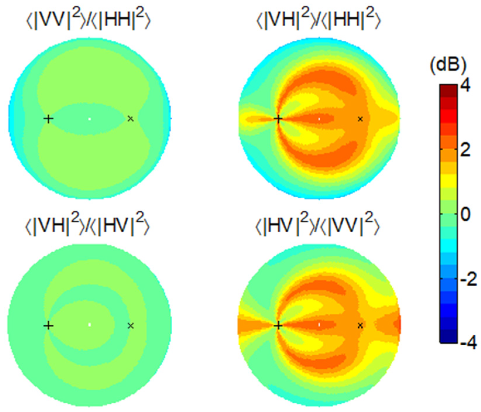
Figure 7 depicts the scattering intensity changes due to the increased randomness in the surface orientation distribution with the concentration parameter reduced from 50 to 30. The intensities in HH and VV largely remain at the same level, except at the low grazing directions. The intensities in HV and VH, however, manifest a clearly enhanced intensity at the geometries where the SPM predicts null returns (Figure 3). This testifies to the fact that the large-scale roughness is primarily responsible for distributing the scattered power to the cross-polarization channels. Figure 8 presents the derived quality factor $I_{SM-\kappa }$ that compares the SMC-induced change against the $\kappa$-induced change. Similarly, the forward scattering directions give better sensitivity in HH and VV to the SMC, but not at very low grazing angles. The bistatic geometry with good sensitivity can also be extended to other non-specular scattering directions using HV and VH, provided that their signals are strong enough.

4.2. Scattering Intensity Ratio

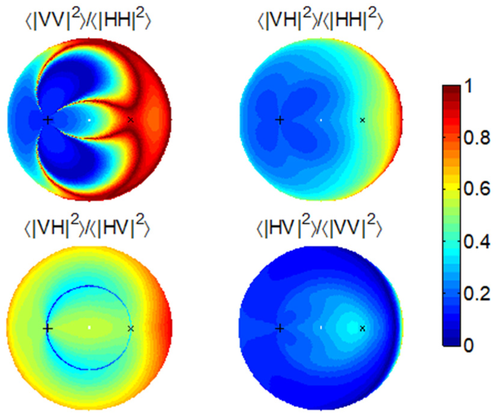
By taking intensity ratios, we hope to cancel out part of the roughness scattering effect. Figure 9 shows that the various ratios generally increase with the SMC. In VV/HH, we can expect substantial increases in the grazing directions, especially in the forward geometry. In VH/HV, a moderate increase occurs only in the grazing directions other than the backward geometry. The greatest change occurs in VH/HH at nearly all scattering geometries.

Figure 10 presents a similar set of plots but in response to higher small-scale roughness. In VV/HH, the change due to higher roughness is very small in the forward scattering directions. In VH/HV, there is very little change, seemingly a favorable result; however, the change due to higher SMC (Figure 9) is also small. In the other ratios involving VH or HV, the changes generally are very large, apparently indicating poor sensitivity to moisture. The quality factors given in Figure 11 clearly show that only the forward grazing geometries can ensure good quality and sensitivity to the SMC.

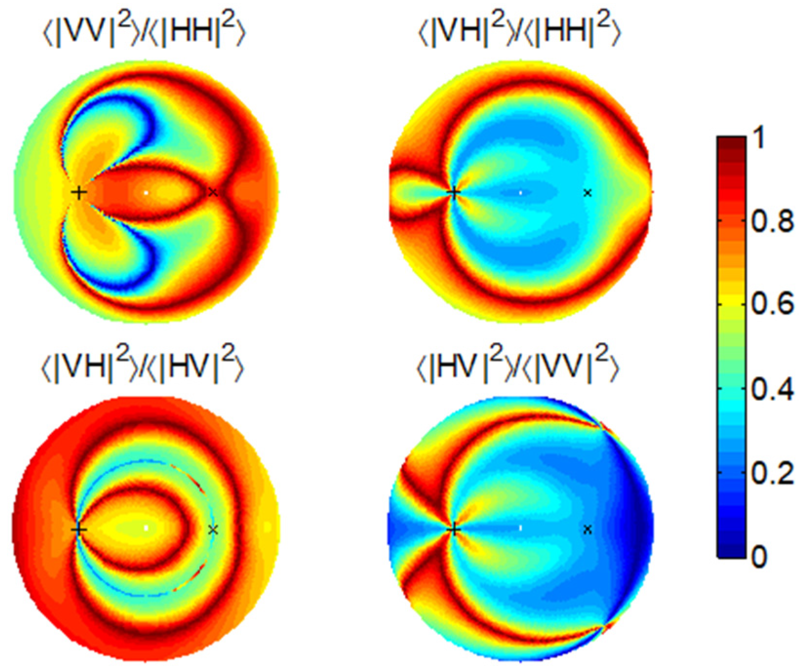
Figure 12 shows that the intensity ratios are relatively immune to the large-scale orientation variation. Accordingly, as indicated in Figure 13, they fare very well under the SMC variation in the presence of a random surface orientation. This agrees with the polarimetric advantages presented in the X-Bragg model [10]. The large increases in VH/HH and HV/VV again are associated with the SPM-predicted nulls.

4.3. Polarimetric Correlation

Both the correlation coefficients and the differential phase shifts among the four polarization channels are not sensitive to changes in either moisture or roughness. The differential phase shifts primarily indicate the number of reflections involved in the scattering process. With negligible variations in the differential phases, the correlation coefficients are also rather stable, even though a tendency is clearly revealed: increasing SMC will reduce ${\rho }_{HHVV}$ but enhance ${\rho }_{HVVH}$, whereas increasing roughness either in terms of $L$ or in terms of $\kappa$ will reduce both. The specific plots are not included here for length considerations.

4.4. Eigenvalues

By mapping the scattering covariance matrix into four uncorrelated, coherent components through eigenvector decomposition, we intend to evaluate how these characteristic scattering components respond differently to moisture and roughness changes.

Overall, the small-scale roughness variation gives rise to larger eigenvalue changes than the SMC variation does, as attested to in Figure 14 through the quality factors. However, we should note that it is the large-scale roughness that causes the covariance matrix to have full rank and distributes the scattered power into multiple scattering components. Manifested over this foundation, the small-scale roughness then affects the specific distribution, particularly by diminishing the dominant component and simultaneously enhancing other, minor components. The SMC variation also affects the distribution but to a much lesser extent.

If $\kappa$ is high, meaning a narrower surface orientation distribution, the impact due to the small-scale roughness becomes smaller, until it eventually disappears in the limiting case of SPM scattering. Nevertheless, in a common natural setting, both the SMC and the small-scale roughness are deeply entangled in the eigenvalues.

In terms of the large-scale roughness, the randomness in the surface orientation distribution greatly shifts the scattered power towards the minor components. All of the quality factors become very low, as shown in Figure 15.

Taking ratios over these eigenvalues may partially mitigate the roughness impact, but we only find limited consistency using $p_4/p_2$ and $p_4/p_3$, which are not likely useful in practice since $p_4$ is very small, reduced by at least −30 dB from the dominant one using our simulation settings.

4.5. Characteristic Polarimetric Parameters

We speculate that the major surface scattering information is contained in the dominant characteristic component, ${\underset{\_}{\mathit{S}}}_1$. It features the polarization state in terms of the polarization orientation angles ${\tau }_{i,s}$and the ellipticity angles ${ϵ}_{i,s}$, as well as the scattering parameters in terms of the scattering ratio $\mathsf{\Gamma }$ and the phase shift $\psi$.

The ellipticity angles likely provide a primary indicator of asymmetrical scattering from the targets and the phase shift is a primary indicator of the number of bounces. They do not have any desired sensitivity to either the moisture variation or the roughness variation.

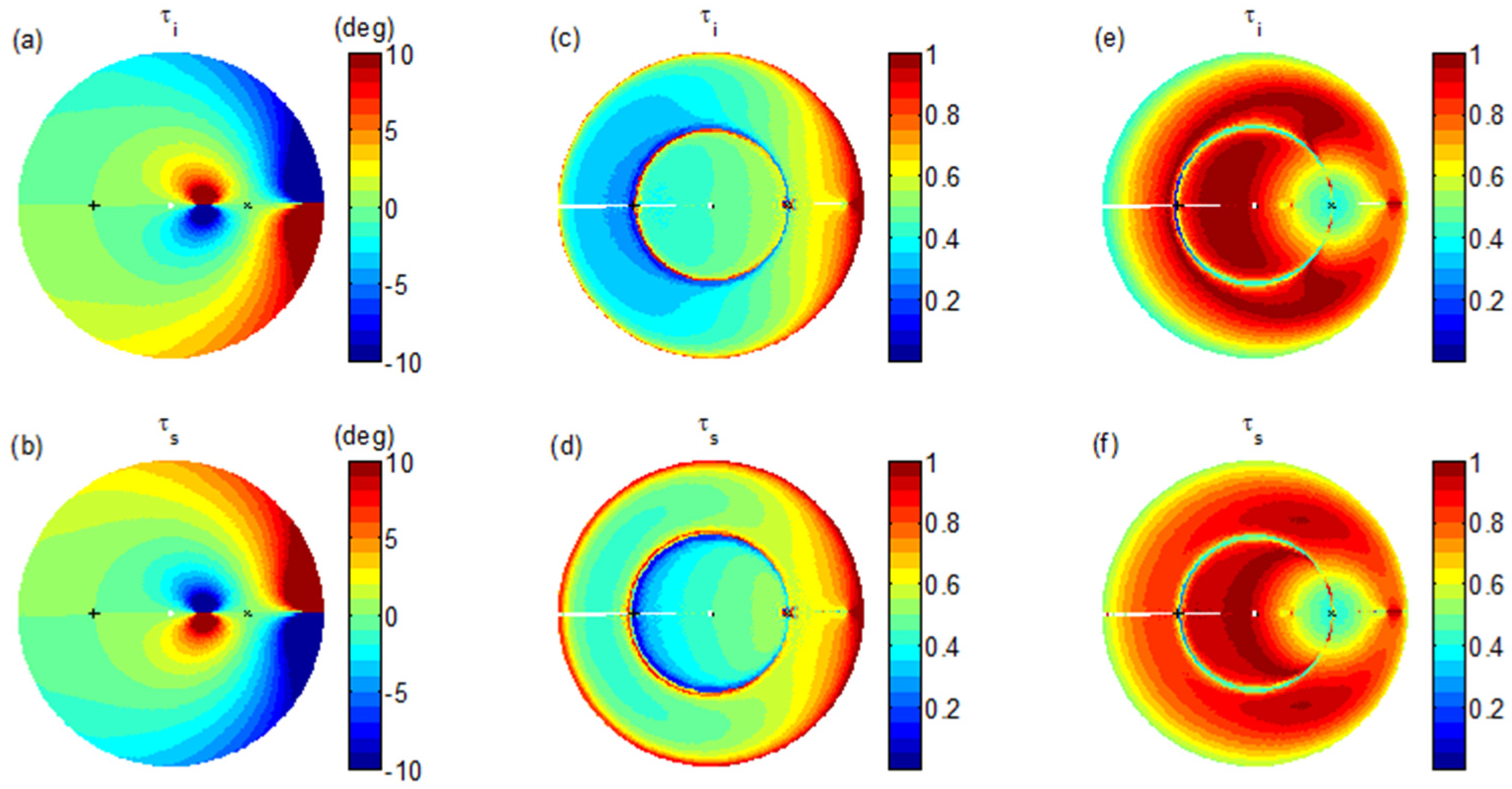
The characteristic POAs are intriguing to use. On the one hand, they vary with the orientation factors of the system polarizations and those of the scattering targets. On the other hand, they are also coupled with the scattering process itself, reflecting a strong dependence on the SMC. Figure 16 illustrates this coupling clearly as the demonstrated changes arise solely from the SMC variation (panels a and b). The changes are fairly large near the forward grazing directions. Comparing them with the changes due to the correlation-length variation from the small-scale surface roughness spectrum, we see a higher quality factor in the forward region and at the low grazing directions (panels c and d). However, we should avoid the low grazing angles in the backward geometry because the SMC-induced changes are very small. When comparing the changes against those due to surface orientation randomness, we actually obtain better quality factors over a wide range of sensing geometries, not only in the specular direction (panels e and f). However, in the near-vertical directions, we also need to be cautious because the SMC-induced changes are very small. In addition, a particular difficulty in using the orientation angles is that we cannot always ascertain that the mean surface is horizontal. In natural terrain, the surface orientation may point to different directions depending on the terrain slope.

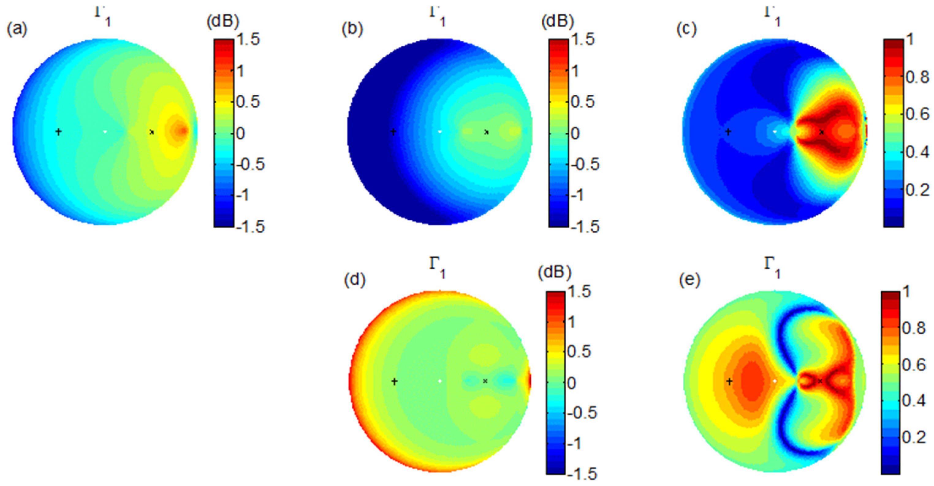
The characteristic scattering ratio, as shown in Figure 17, resembles the general trend of the HH and VV intensities and their ratio VV/HH, implying that it carries the essential scattering information. However, the corresponding changes due to the surface roughness parameters are quite different. With the small-scale variation in terms of the correlation length, a large change exists in the backward directions, whereas a small change exists in the forward directions (panel b). Accordingly, we can expect to obtain good sensitivity to the SMC in a well-organized forward scattering region (panel c). With the large-scale variation in terms of the surface orientation randomness, in the backward directions, the associated change is also small (panel d), where we can expect to obtain some decent sensitivity to the SMC (panel e). Altogether, they highlight a large sector of forward scatter geometries that is suitable for SMC measurement.

5. Remarks and Discussion

The comparable contribution from soil moisture and surface roughness coupled in the rough surface scattering process poses a long-standing challenge for moisture retrieval using SAR observations. A widely acknowledged advantage of using polarimetric radar is its potential ability to mitigate the roughness factor in the scattering response. This is especially true if the surface is only slightly rough, such that the SPM is applicable. However, as the surface roughness increases, the coupling between the soil moisture and surface roughness persists, as demonstrated in previous research performed with AIEM-based simulation. The descriptive parameters for the surface roughness include the type of roughness spectrum, the surface height variation, and the correlation length, each behaving differently in the scattering response and sensitivity.

In this work, we adopted the TSM to explicitly evaluate the role of surface roughness. With the small-scale roughness, the SPM is assumed to be valid locally in the small surface facets. The individual facet size is small enough to ensure a slight surface height variation after adjustment for the local slope, but large enough to produce significant resonant Bragg scattering, which provides the basis for the observed scattered returns. With the large-scale roughness, the mean slope of individual facets produces random polarization rotation and local incidence modulation. The randomness in the polarization orientation angles causes the scattered energy to be distributed into all polarization channels. However, these two scales interact and, in general, should be considered together. Although the SPM predicts roughness-independent polarimetric variables for small facets, the random slope and POA variation change this prospect, reintroducing a polarimetric dependence on the roughness spectrum.

The TSM also allows different polarization channel combinations through polarization basis transformation. Some polarimetric variables have a stronger dependence on moisture variation than on roughness variation. We can define numerous polarimetric variables, but we prefer to select those with physical meaning. To this end, we adopt a special reference frame different from the native polarization bases. This allows us to compensate for the bistatic geometric distortion on the observed polarization channels and regain cross-polarization and co-polarization variables. This is important because, otherwise, the observation would contain a purely geometry-related polarization rotation. In this work, though not exhaustive, we conducted sensitivity experiments over a full list of common polarimetric variables. Their sensitivity to the soil moisture indeed varies greatly, favoring different geometry settings.

Overall, the optimal bistatic geometry is located near the specular direction and the forward grazing directions, especially for scattering intensities or their ratios. This agrees with the previous research findings. The agreement, despite being based on different polarization reference systems, is reasonable because these two reference systems converge in the bistatic plane, which contains both the forward and the specular directions.

As our main objective, we intended to locate non-specular optimal bistatic geometries that mitigate the image resolution concern and determine the associated set of polarimetric variables that can operate there. We also hoped to benefit from the extra polarization channel acquired in the bistatic geometry. We found only partial success, with some limitations. In the presence of a large-scale orientation variation, introduced to accommodate the increased surface roughness, we may attain good sensitivity to moisture in limited non-specular geometries using the minor characteristic components; however, the intensity likely is too low to provide reliable SMC estimates. On the condition of a fixed roughness spectrum, we achieve greater success in wider non-specular geometries using either the cross-polarization channels or the characteristic polarization orientation angles. However, the cross-polarization channels will also have a lower intensity and the characteristic POAs may have biases due to non-zero, terrain-induced mean slopes.

The scattering ratio in the dominant characteristic component appears to be a strong candidate. Although it still points to the same forward geometries near the specular direction, the indicated optimal geometry is better organized and its evaluation is more robust as being independent of the polarization bases.

These limitations do not mean that it is infeasible to estimate soil moisture in non-specular bistatic geometries or it is not beneficial to use polarimetric bistatic observations. Instead, they only indicate the favorable imaging geometries when one of the polarimetric variables is used. For a future endeavor, using multiple polarization channels together may resolve the coupled influence due to moisture and roughness.

6. Conclusions

As bistatic SAR usage opens up the imaging geometry, we explored the bistatic geometry for its optimal deployment to rough surface scattering applications. In this paper, we focused on the sensitivity of the relative polarimetric terms to soil moisture variations. The sensitivity evaluation was based on controlled simulation experiments using the two-scale rough surface scattering model. With this model, we investigated the different impacts associated with the roughness terms at these two scales, namely the correlation length of the Gaussian roughness spectrum and the surface orientation variation. The small-scale variation in terms of the correlation length is found more limiting than the large-scale variation in the polarimetric scattering response for soil moisture retrievals, unless the surface orientation variation is very small. The natively acquired polarimetric observations were always compensated for the geometry-induced polarization rotation. The sensitivity study showed that different polarimetric variables would favor different bistatic geometries for moisture determination. Overall, the forward geometries near the specular direction are more reliable for moisture sensitivity, as revealed in earlier studies. However, we may venture towards other non-specular geometries using cross-polarization variables or characteristic polarization angles. Although we are unable to reach a common range of optimal geometries that is consistent in all scenarios, this study establishes a useful approach to guide bistatic mission planning for future polarimetric collections.