Article

TFCD-Net: Target and False Alarm Collaborative Detection Network for Infrared Imagery

1
School of Information and Communication Engineering, University of Electronic Science and Technology of China, Chengdu 611731, China
2
Laboratory of Imaging Detection and Intelligent Perception, University of Electronic Science and Technology of China, Chengdu 611731, China
*
Author to whom correspondence should be addressed.
Remote Sens. 2024, 16(10), 1758; https://doi.org/10.3390/rs16101758
Submission received: 16 January 2024 / Revised: 10 May 2024 / Accepted: 11 May 2024 / Published: 15 May 2024

Abstract

:
Infrared small target detection (ISTD) plays a crucial role in both civilian and military applications. Detecting small targets against dense cluttered backgrounds remains a challenging task, requiring the collaboration of false alarm source elimination and target detection. Existing approaches mainly focus on modeling targets while often overlooking false alarm sources. To address this limitation, we propose a Target and False Alarm Collaborative Detection Network to leverage the information provided by false alarm sources and the background. Firstly, we introduce a False Alarm Source Estimation Block (FEB) that estimates potential interferences present in the background by extracting features at multiple scales and using gradual upsampling for feature fusion. Subsequently, we propose a framework that employs multiple FEBs to eliminate false alarm sources across different scales. Finally, a Target Segmentation Block (TSB) is introduced to accurately segment the targets and produce the final detection result. Experiments conducted on public datasets show that our model achieves the highest and second-highest scores for the IoU, Pd, and AUC and the lowest Fa among the DNN methods. These results demonstrate that our model accurately segments targets while effectively extracting false alarm sources, which can be used for further studies.

1. Introduction

Infrared Search and Tracking (IRST) systems play a crucial role in various civilian and military applications [1]. They are widely utilized for tasks like pinpointing heat sources during firefighting operations and detecting abnormalities in medical applications [2,3]. These systems make use of emitted or reflected infrared radiation from objects to accomplish target detection, tracking, and identification [4,5]. Their capacity to identify targets becomes particularly valuable in situations where visual identification is hindered or impractical. Examples include scenarios involving targets with camouflage, distant targets, or challenging weather conditions [6].
Detecting infrared small targets presents a significant challenge in IRST applications. These targets are characterized by their small size (typically less than 9 × 9 pixels or constituting less than 0.15% of the field of view) and lack of detailed texture and shape information [7]. Consequently, distinguishing small infrared targets from complex backgrounds becomes challenging, as these backgrounds often contain elements (such as complex terrains, man-made structures, and clouds) that reflect solar radiation in patterns resembling the targets [8,9,10]. As shown in Figure 1, as the complexity of the scenes increases, an increasing number of false alarm sources emerge, leading to reduced saliency of the targets.
Numerous algorithms have been developed for infrared small target detection (ISTD). These algorithms can be broadly grouped into two categories: multi-frame and single-frame methods [11].
Multi-frame methods detect targets by leveraging the relative motion between targets and background across frames in a sequence [12,13,14]. They assume a relatively static background and require the accumulation of information from multiple frames to determine the targets’ location. The advantage of multi-frame methods is that temporal information is used to enhance detection; however, these methods have some limitations: (1) multi-frame methods naturally do not apply to single-frame scenarios; (2) their effectiveness is hindered when the relative motion assumption is not met; (3) in practical applications, there is a strong demand for fast detection using as few frames as possible. Moreover, multi-frame detection can be approached by detecting targets in each frame using single-frame methods and, then, analyzing the trajectories of the detected targets [15]. Therefore, studying single-frame detection methods is prevalent, and we focus on the single-frame method in this paper.
Single-frame detection methods can be grouped into two categories: non-deep learning and deep learning methods. Non-deep learning methods can be further divided into background-suppression methods, target enhancement methods, image structure-based methods, and classifier-based methods. Background-suppression methods segment target regions by subtracting an estimated background from the input image [16,17,18]. Target-enhancement methods employ calculations of local contrast and saliency to search for or amplify the target regions [19,20,21,22,23,24]. Image-structure-based methods assume a mathematical model of low-rank background and sparse targets and solve for the target region through optimization techniques [25,26,27,28]. Classifier-based methods are typically combinations of candidate extraction, feature extraction, and feature classification [29,30]. These non-deep learning methods use interpretable mathematical models to model the target and background; however, their modeling heavily relies on prior knowledge, so their effectiveness is often compromised in complex scenes, as manually designing constraints and features to accurately discern between targets and false alarms can become problematic.
Deep learning methods automate the process of extracting features for targets using deep neural networks (DNNs). Among them, target-detection networks estimate bounding boxes to approximate the location of small targets [31,32,33,34], while target-segmentation networks address target detection as a semantic segmentation problem [35,36,37,38,39], aiming to accurately identify the location of small targets at the pixel level. The target-segmentation approach is gaining popularity in research due to its ability to more precisely identify regions containing small targets [7], indicating a promising direction for future progress. Although deep learning methods have achieved impressive progress in ISTD [40,41,42,43,44,45], there are notable drawbacks. Firstly, existing methods mainly concentrate on modeling the targets, disregarding the modeling of false alarm sources, which also carry useful information, while in practical scenarios, the detection of infrared small targets against densely cluttered backgrounds requires a combined effort to eliminate false alarm sources and detect the targets in order to minimize the false alarm rate. Additionally, the opaque nature of DNNs is a significant limitation, for interpretability is crucial due to the fact that ISTD is a risk-sensitive task.
Taking into account the practical needs and the advantages and drawbacks of the aforementioned methods, the objectives of this research are to employ DNN techniques that make use of information from both targets and false alarm sources to achieve accurate and robust target segmentation, while maintaining interpretability.
To achieve these objectives, we present the Target and False Alarm Collaborative Detection Network for Infrared Imagery (TFCD-Net). Our network addresses the need to incorporate information from false alarm sources by utilizing specialized False Alarm Source Estimation Blocks (FEBs). In order to enhance interpretability, we have designed the overall framework of our network to resemble the background suppression process employed in non-deep learning methods. Specifically, the network first suppresses false alarm sources by subtracting the results of multiple FEBs from the input image and, then, proceeds to segment the targets using a Target Segment Block (TSB).
The major contributions of this research can be summarized as follows:
  • We propose a framework that effectively models both targets with TSB and false alarm sources with FEBs. This approach aims to address the challenges posed by complex and cluttered backgrounds while maintaining interpretability.
  • We introduce a dedicated FEB to estimate potential false alarm sources. By integrating multiple FEBs into the framework, false alarm sources are estimated and eliminated on multiple scales and in a blockwise manner. This block not only enhances the accuracy of our method, but also can serve as a preprocess module to suppress false alarm sources for other ISTD algorithms.
  • Extensive experiments on public datasets validated the effectiveness of our model compared to other state-of-the-art approaches. In addition to accurately detecting targets, our model can produce multi-scale false alarm source estimation results. These estimations are not just incidental outcomes; they can be used to generate false alarm source datasets that can contribute to further studies in the field.

2. Related Works

2.1. Image-Structure-Based ISTD

Numerous non-deep learning algorithms have been proposed for ISTD; among them, image structure-based methods have achieved high performance and provide solid mathematical foundation for ISTD. Image-structure-based methods typically represent infrared images using Equation (1):
f D ( x , y ) = f T ( x , y ) + f B ( x , y ) + f N ( x , y ) ,
where f D , f T , f B , f N , and ( x , y ) denote the original image, the target image, the background image, the noise, and the pixel location, respectively. This representation suggests that an infrared image can be expressed as a superimposition of three components: target, background, and noise component. Therefore, ISTD is equivalent to separating the target component from the background and noise components.
To separate the target component, image-structure-based approaches assume that the background of an infrared image is low-rank, while the small target is sparse. By formulating constraint equations for the background and target, mathematical optimization techniques are employed to separate the input image into these two components. Then, target areas are extracted by binary segmentation. For example, in NRAM [46], the weighted l 1 -norm is used to constrain the target, and the l 2 , 1 -norm is used for noise; in the PSTNN [47], the partial sum of tensor nuclear norm joint weighted l 1 -norm is used to constrain the background in the tensor space; in SRWS [48], a self-regularization item is used to constrain the background, and overlapping edge information is used to constrain the target. These constraint-optimization problems are then solved by applying the alternating direction method of multipliers.
Image-structure-based methods focus on discovering improved mathematical models to represent elements of an infrared image. These mathematical representations offer interpretability for the methods. However, a drawback of image-structure-based methods is that, due to their reliance on manual modeling, their robustness and generalizability are hindered in complex scenes.

2.2. Deep Learning-Based ISTD

In contrast to non-deep learning methods, DNN models are data-driven, and the features and relationships between the input and desirable output are automatically learned during training.
Deep learning-based ISTD methods are developed from visible light image target detection and segmentation networks [49,50,51,52,53]. Efforts include applying UNet [54] with reduced input channels for ISTD. UNet is composed of a progressive downsampling encoder, a progressive feature concatenation, and an upsampling decoder. In ACM [35], an asymmetric contextual modulation module is used to exchange both high-level and low-level information to enhance the encoder–decoder framework. In ALCNet [43], multiscale local contrast blocks are used to extract local contrast feature maps, and bottom-up attentional modulation modules are used to encode low-level features into high-level features. In ISTDUNet [45], merge connections are employed to replace the skip connections between the encoder and decoder to improve UNet. In DNANet [44], dense nested attention blocks are used to extract and fuse features at multiple layers. In RDIAN [40], special convolution layers that resemble the local-contrast-extraction process are designed to reduce the parameter size and achieve fast detection.
Although automatic feature extraction and relationship mapping enable DNN models to achieve high accuracy and generalization, a limitation of existing deep learning methods is that they often focus solely on designing structures to model the target component. However, there has been limited effort in modeling and reducing false alarm sources, which actually contain valuable information. By combining knowledge from image-structure-based methods and making use of false alarm source modeling, the performance and interpretability of deep learning-based ISTD methods can be further improved.

3. Proposed Method

3.1. Overall Framework

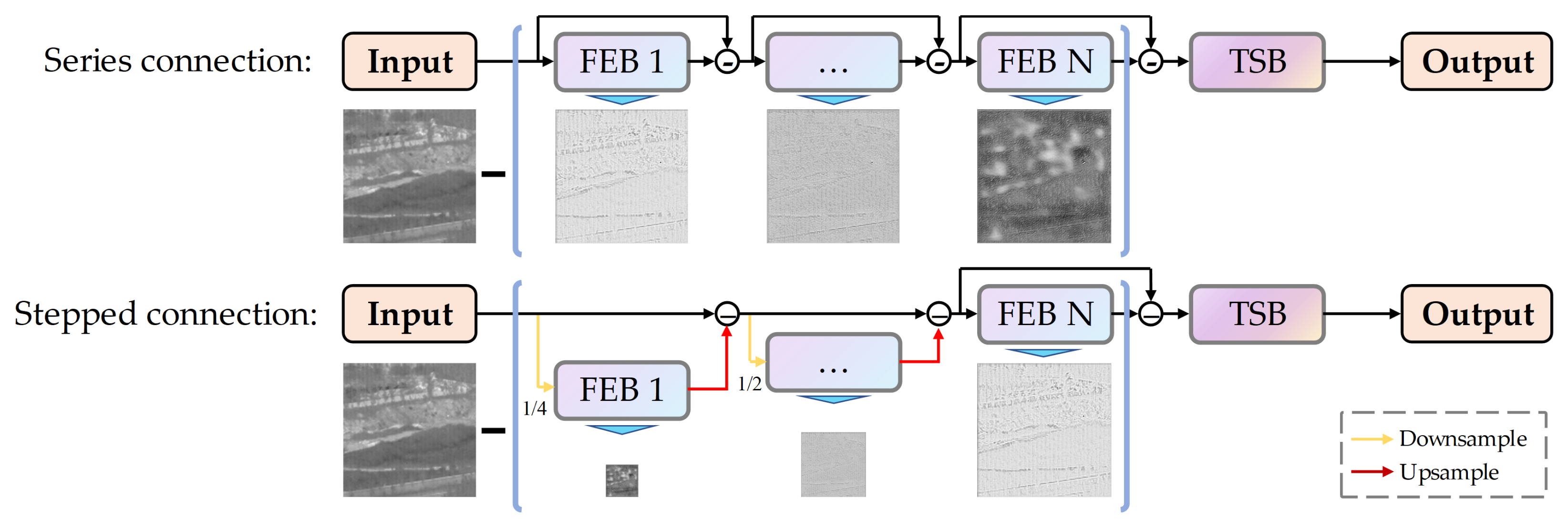
The overall framework of the proposed TFCD-Net is depicted in the upper section of Figure 2. It is designed to suppress false alarm sources in a multi-stage process before segmenting the target. The suppression is achieved through the implementation of multiple FEBs, each functioning as a residual block [55], where the input is subtracted by the output, then the result serves as the input for subsequent blocks. Although the number of these suppression stages can be varied, experiments have shown that 2 to 3 stages are usually sufficient to meet the requirements of subsequent high-performance target segmentation. A series connection configuration of the blocks is illustrated in the upper section of Figure 3.
We investigated an alternative multiscale, multi-stage structure, as shown in the lower section of Figure 3. Although this configuration was found to be less effective in Section 4.2, we believe that retaining the information could be beneficial for future studies. In this configuration, three FEBs operate at different scales: 1/4, 1/2, and the original scale. The formula is as follows:
O FEB k = Up 2 ( n k ) × bilinear FEB MaxPool 2 ( n k ) ( I FEB k ) ,
where Up x bilinear is factor x bilinear upsampling, MaxPool x is factor x max pooling, k = 1 , 2 , , n 1 , and n is the number of FEBs. This design strategy is aimed at enabling the network to suppress false alarms progressively from coarse to fine levels. In this framework, the output of each FEB is upsampled back to the original scale before it is subtracted by the output of the previous stage, ensuring that no original image information is lost during the downsampling process.
The role of the FEB is to suppress false alarm sources, and it does not precisely extract the shape of the targets. To accurately segment targets from the false alarm-source-suppressed result, a semantic segmentation network is employed as the segmentation head. While there are various choices for the segmentation head, we utilized the same architecture as the FEB for the TSB, but the output of the block is processed through a sigmoid activation function to ensure the output pixel values are confined between 0 and 1. Unlike the TSB outputs, FEBs do not restrict their outputs with an activation function. Instead, false alarm subtraction is performed using a linear rectification function (ReLU) [56] as the activation function to constrain negative values. The overall process is shown in Equation (3):
  O 1 = ReLU FEB 1 I 1   O k = ReLU O k 1 FEB k O k 1 , k = 2 , 3 , , n O final = Sigmoid O n TSB O n
where I 1 is the original image, O k is the output of the k-th stage, FEB k is the k-th FEB with the aforementioned downsampling and upsampling if in stepped connection as in Equation (2), and O final is the final target segmentation result.

3.2. False Alarm Source Estimation Block

The FEB is an important component of the proposed TFCD-Net framework, designed to accurately estimate false alarm sources. As shown in Equation (1), the estimation of false alarm sources involves the subtraction of the target component from the background. Given the small size of infrared small targets, this estimation process is comparable to image denoising, which aims at removing small objects from the image.
Typically, denoising networks use stacked convolutional layers or encoder–decoder architectures similar to UNet [57,58]. The multiscale structures are beneficial as they capture background patterns in a wider area, making the estimation more complete. In consideration of these studies, we introduce a multiscale architecture for modeling false alarm sources, as shown in the lower section of Figure 2.
Within the FEB, the original image is first downsampled by 1 / 2 , 1 / 4 , and 1 / 8 , resulting in a total of 4 scales of input images as follows.
O pool , k = MaxPool 2 ( k 1 ) I FEB ,
where O pool , k is the downsampled image of the k-th scale, k = 2 , 3 , , n . I FEB is the input of the FEB. MaxPool 2 ( k 1 ) performs max pooling of factor 2 ( k 1 ) .
Subsequently, two double-convolution operations are performed on each scale, forming the encoder component of the FEB. The double-convolution block is depicted in the bottom-right corner of Figure 2, consisting of two sets of convolutional layers, batch normalization layers, and ReLU activations. The formula is as follows:
O d c = ReLU BN Conv 3 × 3 ReLU BN Conv 3 × 3 ( I d c ) ,
where O d c and I d c are the output and input of the double-convolution block.
The decoder component of the FEB uses a UNet-like decoder structure for progressive upsampling and feature fusion: for each scale, upsampling by a factor of 2 is initially performed, followed by feature concatenation with the previous level. The formula is as follows:
I de = O k Up 2 × bilinear ( O k + 1 ) ,
where O k and O k + 1 are the k- and (k + 1)-th scale, k = 1 , 2 , , n 1 . ⊕ represents the concatenation operation. Up 2 × bilinear indicates bilinear upsampling by a factor of 2.
The concatenated feature is then forwarded through two double-convolution operations. This upward feature fusion continues until the original image size is reached, and the output image is obtained through a 1-channel 1 × 1 convolution operation to produce a single-channel output. The FEB uses max poolings for downsampling, bilateral filters for upsampling, and 64-channel 3 × 3 convolution kernels for all double-convolution operations. There is no activation function used after the final convolution layer, as activations between blocks are placed in false alarm subtractions, as in Equation (3).

3.3. Loss Function

In the field of ISTD, the commonly used loss function is the soft Intersection over Union (IoU) loss function [59], which is a loss function based on the IoU. The IoU is a common evaluation metric for image-segmentation tasks, used to measure the overlap between predicted and ground truth segmentations, defined as the ratio of the intersection of the prediction and the ground truth to their union. However, since the IoU is not differentiable, it is hard to use directly as a loss function in the training process of deep learning models. Instead, a variant of the IoU, the soft IoU, is used to design the loss function. The soft IoU is a differentiable approximation of the IoU and is defined in Equation (7):
L S I ( P , Y ) = 1 i = 1 N P i · Y i + ε i = 1 N P i + i = 1 N Y i i = 1 N P i · Y i + ε ,
where P and Y, respectively, denote the predicted output of the network and the ground truth, ε represents the smoothing factor, and N indicates the total number of samples. The incorporation of the smoothing factor is a common strategy to prevent the denominator of the loss function, which includes division, from becoming zero. To ensure that the inclusion of the smoothing factor does not significantly affect the actual loss value, ε is typically chosen to be very small.
The soft IoU loss provides several advantages in infrared small target segmentation. Unlike the mean-squared error (MSE) and cross-entropy (CE) losses, which calculate the loss function for each pixel independently, the IoU-based loss takes into account the spatial arrangement of pixels. This approach places greater emphasis on accurately locating targets. Moreover, in tasks involving the segmentation of small targets in infrared images, the number of background pixels greatly outweighs the number of target pixels, resulting in a class imbalance. By utilizing IoU-based calculations, the influence of this imbalance is reduced, thereby enhancing the network’s IoU performance.
However, in practical applications, the soft IoU loss function also has limitations, such as maximizing the IoU may not necessarily result in clear edges. To address unclear edges, a weighted binary cross-entropy (WBCE) loss function designed for single-class small target segmentation is formulated as in Equation (8):
L W B C E ( P , Y , W ) = 1 N i = 1 N W i [ Y i · log ( P i ) + ( 1 Y i ) · log ( 1 P i ) ] ,
where P and Y, respectively, denote the predicted output of the network and the ground truth, W represents the weight map, and N indicates the total number of samples. The weights W are applied on a per-pixel basis to the binary cross-entropy (BCE) loss, an approach that serves to emphasize specific regions. The weights are designed as Equation (9):
W = D ( C ( Y ) , E ) ,
where C represents the Canny edge detection operator, D denotes the morphological dilation operation, and E is a square structural element measuring 2 × 2 .
The total loss function of this method is as given in Equation (10):
L ( P , Y , W ) = L S I ( P , Y ) + α L W B C E ( P , Y , W ) ,
where α is the weight coefficient.
The idea behind the loss function design is to use the soft IoU function as the core and improve the performance of the loss function through edge loss to achieve stable segmentation of small targets.

4. Experiments

4.1. Settings

In the experiments, two public datasets were used: the NUAA-SIRST dataset [35] and the NUDT-SIRST dataset [44]. The NUAA-SIRST dataset consists of 427 images; the NUDT-SIRST dataset contains 1327 images. These images represent various common infrared scenes, such as clouds, sea surfaces, urban environments, and ground scenes. They are relevant for both terrestrial and aerial ISTD tasks. The resolution of all images in the datasets is 256 × 256 pixels. We evenly divided the datasets into training and testing sets, with a split ratio of 50%.
The performance of the algorithms and networks was evaluated using various metrics. The key evaluation metrics used were the probability of detection ( P d ), false alarm rate ( F a ), intersection over union ( I o U ), and receiver operating characteristic (ROC). The definitions of these metrics are as follows.
Probability of detection ( P d ): Measures the ability of detecting true targets on the target level. Defined as the ratio of the number of correctly detected targets over true targets as follows:
P d = T c o r r e c t T A l l ,
where T c o r r e c t is the number of correctly detected targets and T A l l is the number of true targets. A higher score indicates better detection capability.
False alarm rate ( F a ): Measures the rate of detecting false targets on the pixel level. Defined as follows:
F a = F P F P + T N ,
where F P and T N are pixel-level false positive and true negative detections, respectively. A lower score indicates fewer false positive detections.
Intersection over union ( I o U ): Measures the accuracy of detection on the pixel level. Defined as the area of overlap between the predicted and the ground truth targets divided by the area of their union as follows:
I o U = A I A U ,
where A I is the area of intersection and A U is the area of union. Area is calculated as the number of pixels. A higher score indicates higher accuracy segmenting the targets.
F1-score: Measures the balanced score considering both precision and recall as follows:
P r e c i s i o n = T P / ( T P + F P ) R e c a l l = T P / ( T P + F N ) F 1 = 2 ( P r e c i s i o n · R e c a l l ) / ( P r e c i s i o n + R e c a l l )
where T P , F P , and F N are the pixel-level true positive, false positive, and false negative detections, respectively. A higher score indicates higher overall detection performance.
Receiver operating characteristic (ROC): Measures the robustness of detection. Defined as the curve of the false positive rate (FPR) to the true positive rate (TPR). To improve the effectiveness of evaluation, a series of 3D ROC curve-derived evaluation metrics proposed in [60,61] were used. Among the metrics, higher area under the curve (AUC) scores (except the lower score for AUC F , τ ) indicate better robustness.
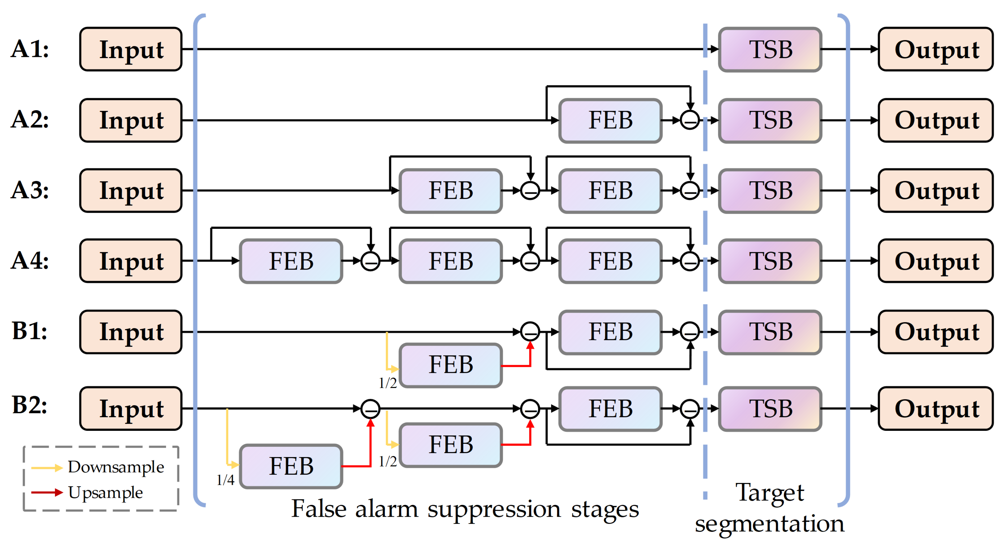
For the model setup, the network structures displayed in Figure 4 were employed in the ablation study; structure A3 in Figure 4 was employed in the comparative experiments. Regarding the loss function, the coefficient α was set to 0 during the initial 50 training epochs and was adjusted to 0.2 thereafter. The optimization algorithm used was Adaptive Moment Estimation (ADAM). The initial learning rate was set at 0.001 and scheduled to decay by a factor of 0.1 every 50 epochs. The training regimen spanned 200 epochs with a batch size of 8.
Illustrative samples from the datasets are showcased in Figure 5 and Figure 6, providing visual context to the types of infrared images used in the experiments.

4.2. Ablation Experiments

The overall framework of the network was subjected to ablation testing, which included evaluating six different structural configurations, as shown in Figure 4. Type-A networks are represented in a serial connection, composed of 0, 1, 2, or 3 FEBs coupled with a single TSB. Type-B networks feature a stair-step connection consisting of either 2 or 3 FEBs and a single TSB. The intent behind these experiments was to identify the optimal number of stages for background suppression and to validate the effectiveness of the stair-step connection approach.
The six aforementioned network structures were trained and tested on two datasets: NUAA-SIRST and NUDT-SIRST. The outcomes of these trials are presented in Table 1.
The results outlined in Table 1 indicate that employing a stair-step connection (Type-B networks) does not enhance network performance. Contrarily, an increase in the number of stages correlated with a decline in the performance metrics, a trend that was particularly pronounced with the NUDT-SIRST dataset. This dataset typically features smaller targets, and it is hypothesized that the Type-B network’s upsampling and downsampling procedures might introduce disturbances to the edge characteristics of these targets. Though Type-B structures have shown less effectiveness, we consider that retaining the records in this section could be a reference and beneficial for future studies.
For Network Type-A, incorporating two FEBs resulted in the best performance. Increasing the number of blocks beyond that did not lead to further enhancements in network capacity. Therefore, based on these findings, we chose the network structure A3 for comparative testing in this section.

4.3. False Alarm Source Estimation Capability

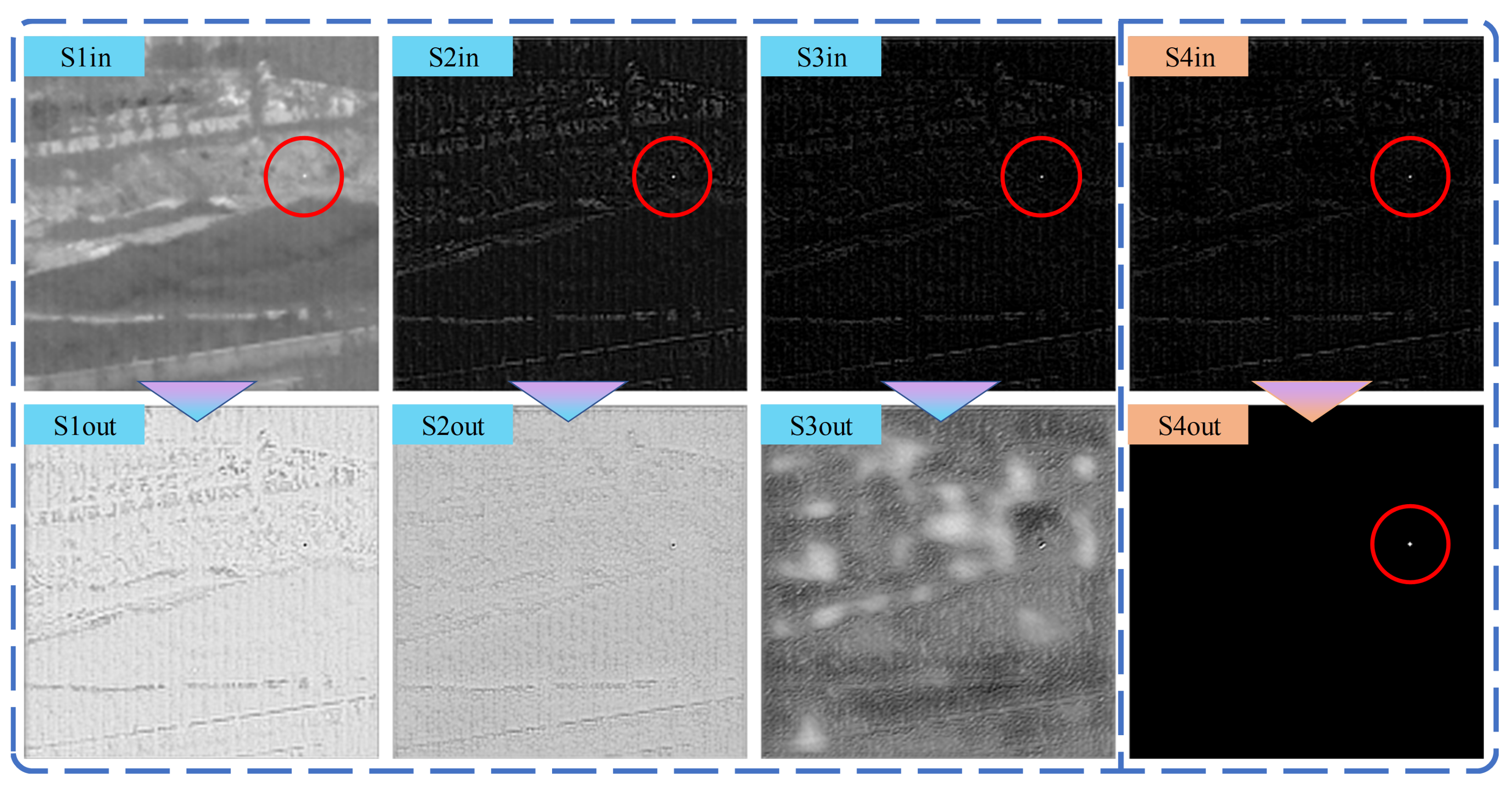
Experiments were carried out to validate the ability of the proposed model to estimate false alarm sources. To conduct a detailed analysis, the A4 framework was selected based on its performance in the ablation experiments. The various stages of the model’s input and output, depicted in Figure 7, were examined. These stages include the network input, which corresponds to the original image (S1in), and the network output (S4out).
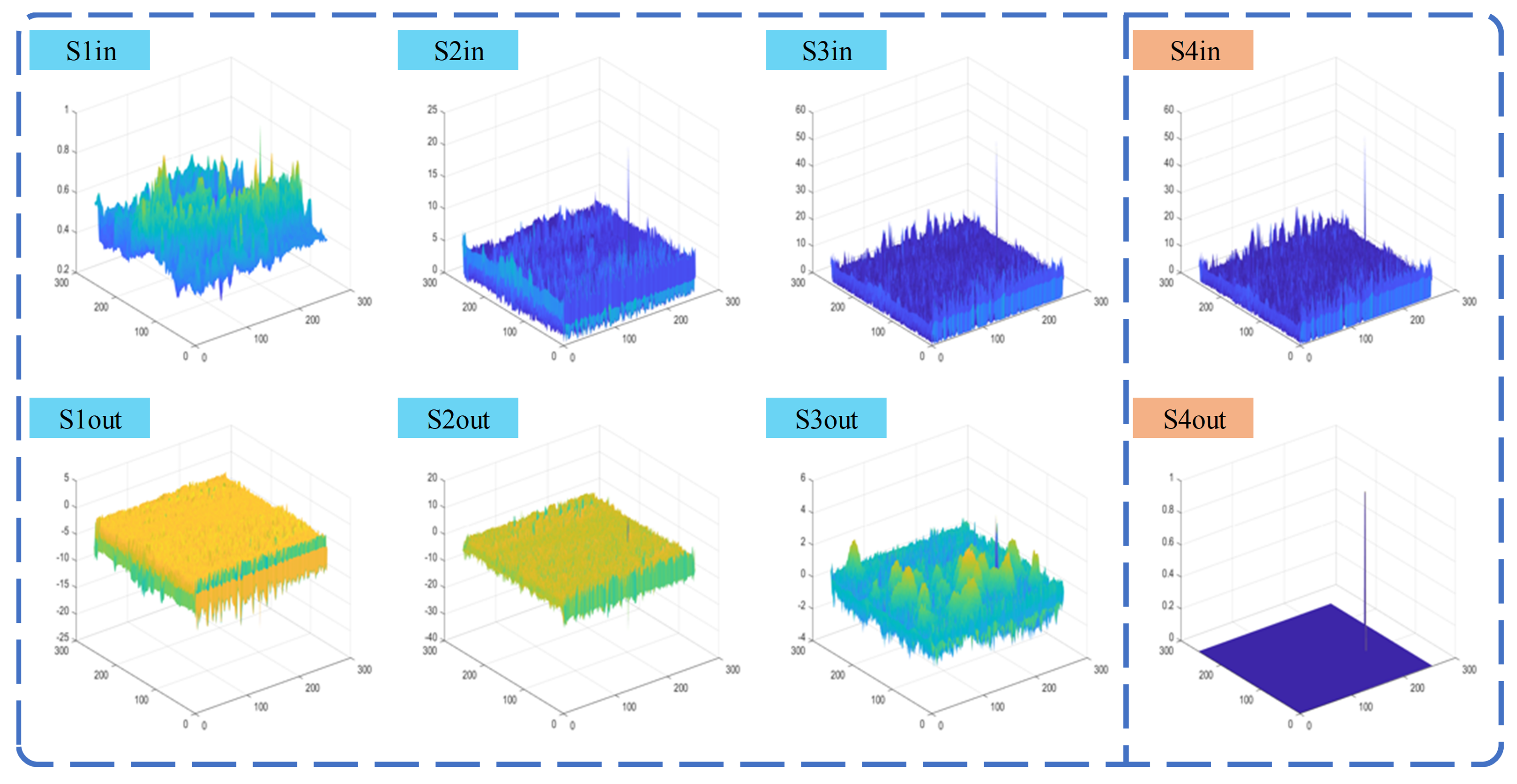
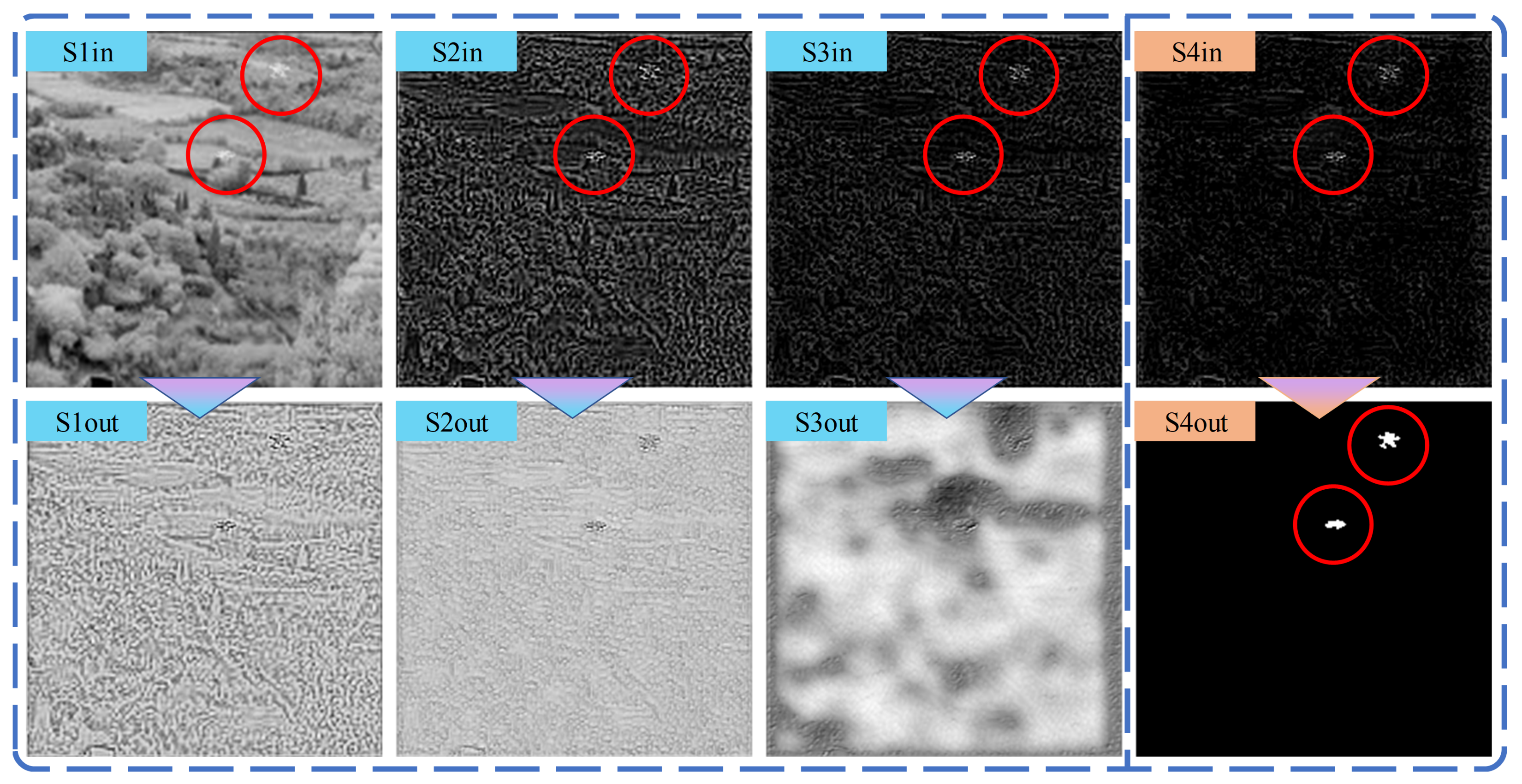
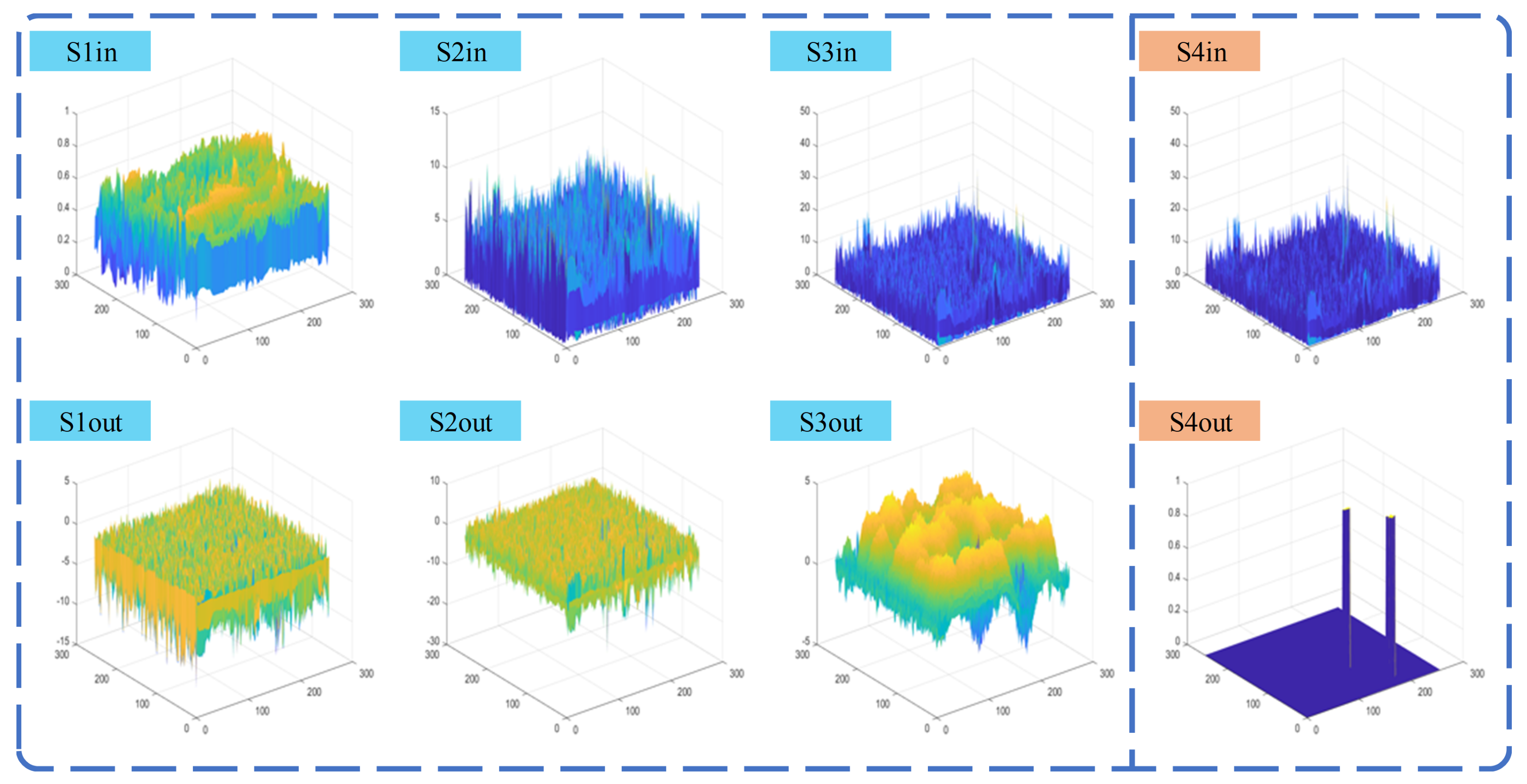
The experiments were performed on multiple scenes, with results depicted in Figure 8, Figure 9, Figure 10 and Figure 11. Figure 8 and Figure 10 show two dense clutter scenes from the NUDT-SIRST dataset. In these figures, the first row demonstrates the inputs of each stage, while the second row shows the corresponding outputs, with red circles indicating the targets. The 3D visualization of these scenes are, respectively, presented in Figure 9 and Figure 11.
From Figure 8 and Figure 10, it is evident that the false alarm sources were progressively suppressed from S1in to S4in; meanwhile, the target regions were preserved. This was achieved by the gradual suppression of non-target edge areas, making targets more salient and easier for the final TSB to process. The outputs from S1out to S3out correspond to the outputs from the FEBs. It can be observed that the suppression of false alarm sources progresses from finer to coarser details and from higher to lower frequencies. This suggests that each stage of the network estimates and suppresses the most salient non-target edge regions. By S3 stage, where most high-frequency regions have already been suppressed, the FEB begins estimating the low-frequency fluctuations in the background. It should be noted that the FEBs do not suppress the target area at any stage, as is evident from S1out, S2out, and S3out, thus ensuring the preservation and increasing saliency of the target. This characteristic is particularly evident in the images of S2in, S3in, and S4in depicted in Figure 9.

4.4. Comparative Experiments

The proposed TFCD-Net was evaluated and compared with state-of-the-art methods, including the optimization-based methods NRAM [46], the PSTNN [47], and SRWS [48], as well as the deep learning methods ACM [35], ALCNet [43], RDIAN [40], UNet [54], ISTDUNet [45], and DNANet [44].
For the non-deep learning methods, the original parameters from their respective publications were employed. The DNN models were trained using the ADAM optimizer with a batch size of 8, an initial learning rate of 0.001 for 200 epochs, and a learning rate decay by a factor of 0.1 every 50 epochs. The soft IoU loss was used for training the DNN models.
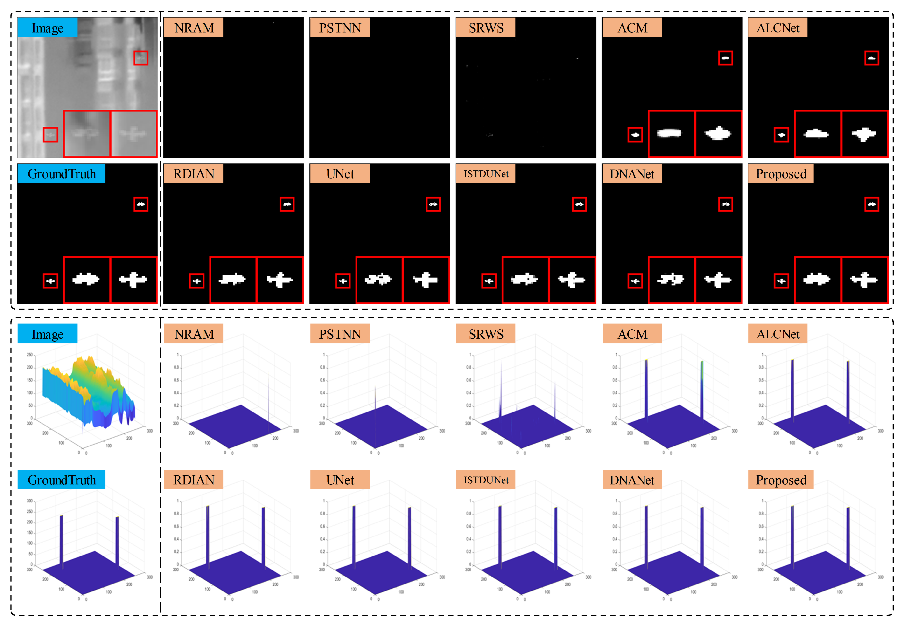
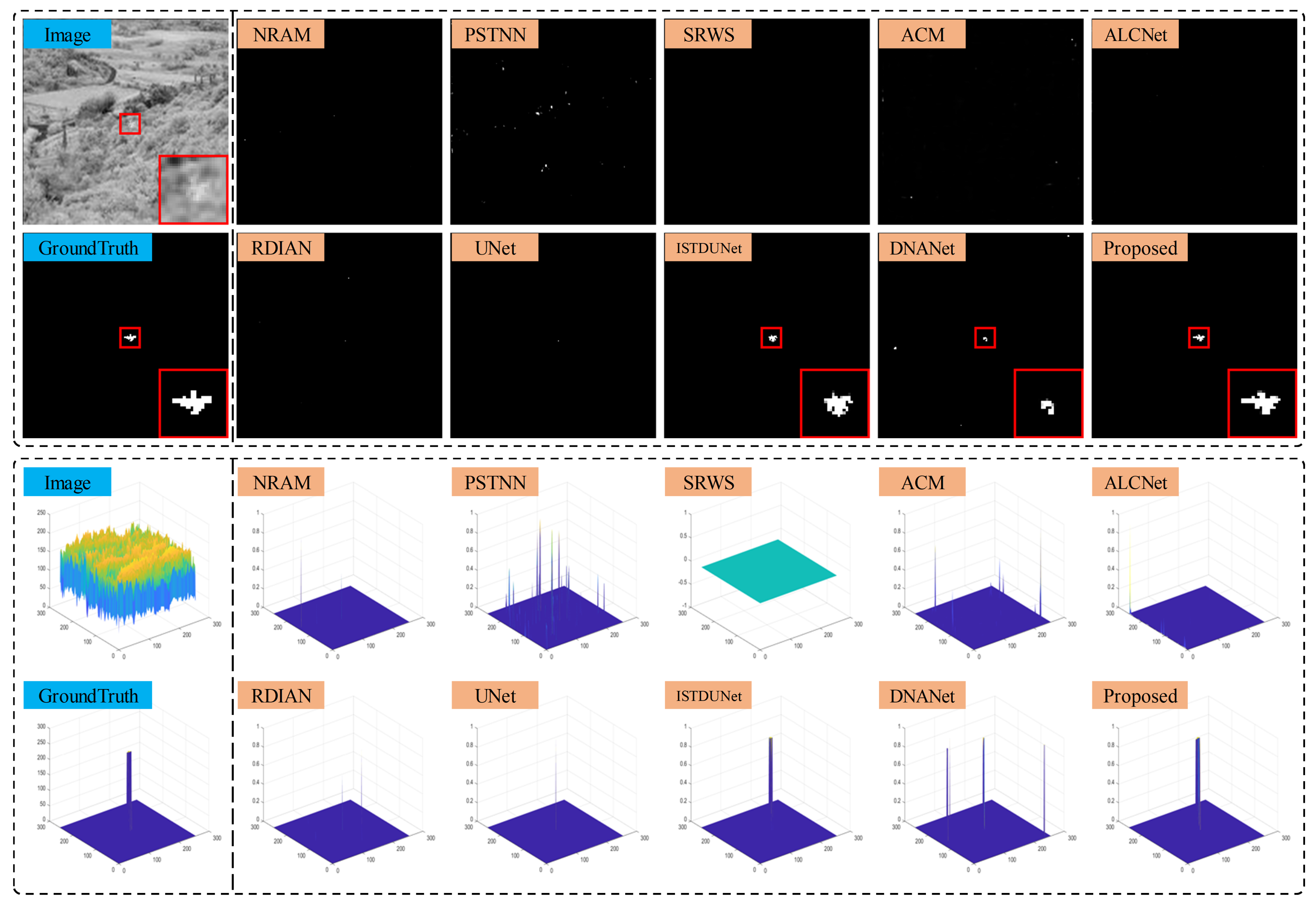
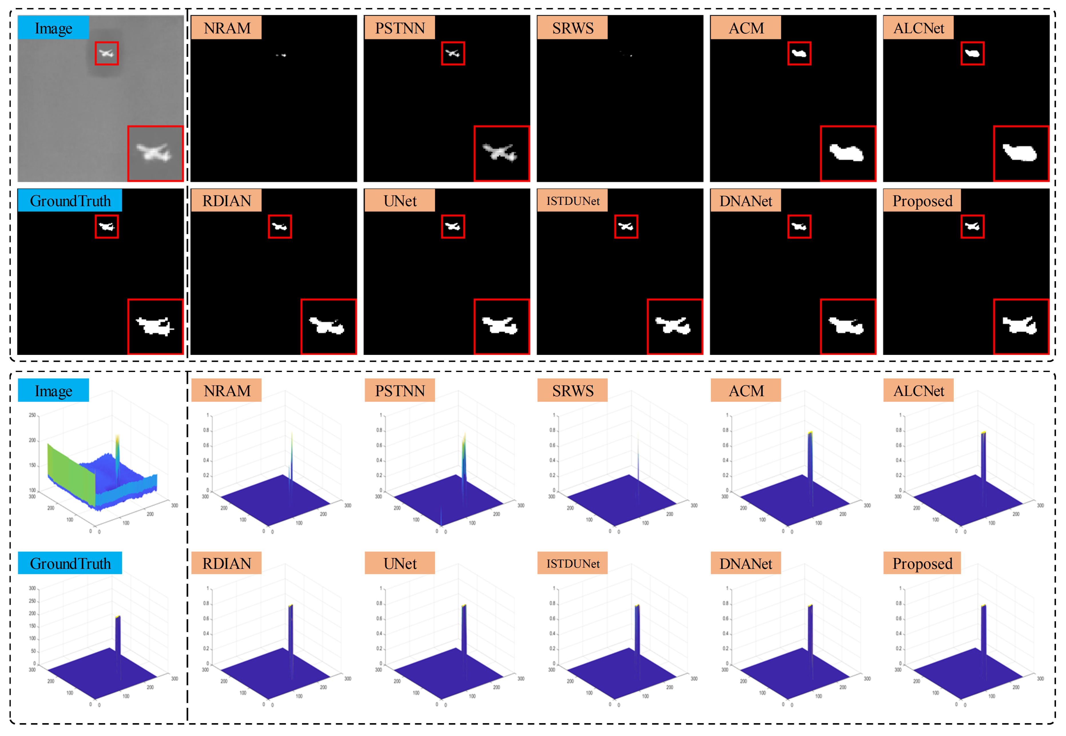
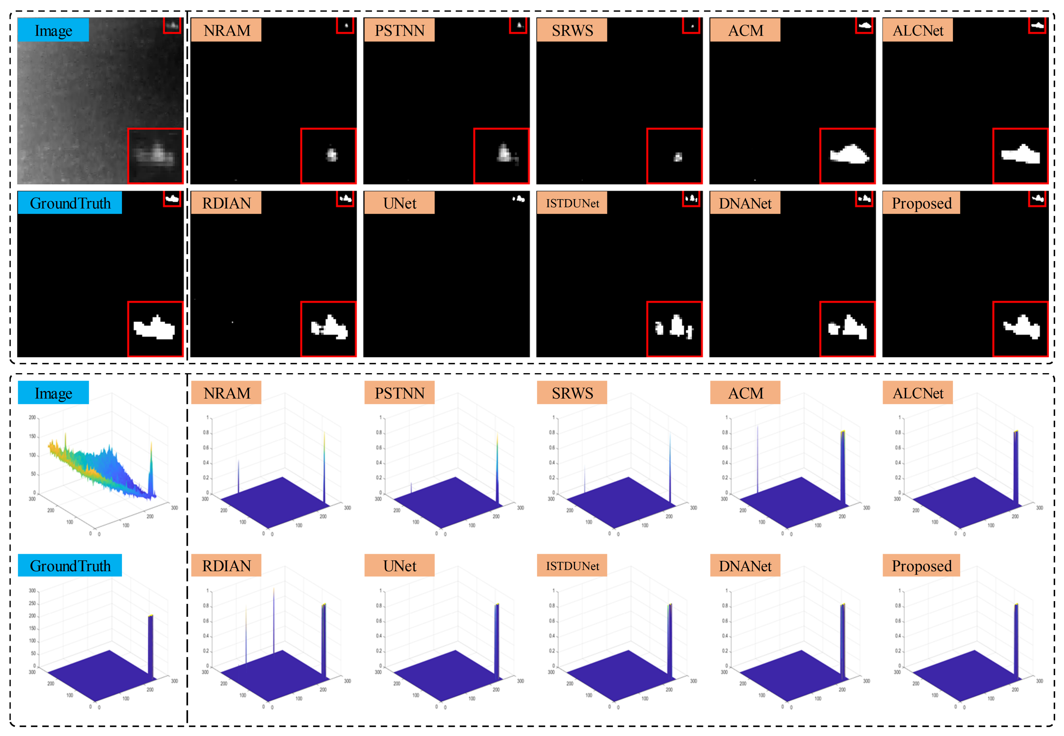
The performance of the proposed TFCD-Net and the comparison methods is demonstrated on six representative scenes from the NUAA-SIRST and NUDT-SIRST datasets. The output results and 3D visualizations for these scenes are depicted in Figure 12, Figure 13, Figure 14, Figure 15, Figure 16 and Figure 17. It can be observed that, in scenes 1 to 5, the three non-deep learning methods failed to detect some targets, highlighting the insufficient stability of manually modeling in complex environments. This was particularly evident when the assumptions of sparsity for targets and low rank for backgrounds were not met, such as in heavily cluttered scenes and scenes with larger targets. Figure 14 showcases a complex scene where most comparison methods failed to detect the target. While the ISTDUNet and DNANet models detected the target, they lacked precision in segmentation. In contrast, the proposed model was capable of accurately segmenting the target. In Figure 16, larger targets posed a challenge for models like ACM and ALCNet, which produced imprecise contours.
In Figure 17, RDIAN, UNet, ISTDUNet, and DNANet segmented the single target into multiple parts, potentially affecting precise localization and subsequent identification in practical applications; for instance, UNet’s detection was more than three pixels away from the true center of the target, which is significant given the small size of the targets. The proposed TFCD-Net performed well across all six scenes, especially on the more complex NUDT-SIRST dataset, as shown in Figure 12, Figure 13 and Figure 14.
For a quantitative assessment, Table 2 and Table 3 present the comparative test results of the proposed TFCD-Net and other methods on the NUAA-SIRST and NUDT-SIRST datasets.
From Table 2 and Table 3, it can be observed that, for the P d value, the proposed TFCD-Net achieved the highest score on the NUDT-SIRST dataset, and the second-best on the NUAA-SIRST dataset, comparable to the performance of DNANet, confirming its effectiveness in detecting small targets alongside the leading methods.
For the I o U and F 1 scores, the proposed method achieved the highest on the NUDT-SIRST dataset and the second-best on the NUAA-SIRST dataset, second to RDIAN, which demonstrates a slightly more precise target segmentation. The RDIAN model, with its MPCM-inspired convolutional kernel design, showed limited generalizability on the NUDT-SIRST dataset, where the proposed TFCD-Net maintained its high performance.
For the F a score, the proposed method outperformed all other deep learning methods on both datasets, demonstrating its superior capability in suppressing false alarms. It is important to note that the SRWS algorithm, while not a DNN-based approach, showed a significantly lower F a score, which may be attributed to its lower I o U and P d values, suggesting a tendency to output smaller target areas, which can also be inferred from the results in Figure 12, Figure 13, Figure 14, Figure 15, Figure 16 and Figure 17.
The robustness of the methods was analyzed by plotting the 3D ROC-derived curves shown in Figure 18 and Figure 19 and calculating the AUC values as presented in Table 4 and Table 5. The proposed TFCD-Net achieved the best score on the NUDT-SIRST dataset and showed competitive AUC scores among DNN approaches on the NUAA-SIRST dataset. A low score for AUC F , τ and a high score for other AUC metrics suggest effective background suppression and strong target responses, which indicate the robustness of the proposed TFCD-Net.
Further analysis of Table 2, Table 3, Table 4 and Table 5 and Figure 18 and Figure 19 indicates that the performance of deep learning methods significantly exceeds that of non-deep learning methods in all metrics except the Fa value. Non-deep learning model-driven algorithms are constrained by the need to manually model small target features, applying constraints such as shape or sparsity and extracting specific components from images. While such designs do not rely on large datasets, they are limited in their scope due to their modeling bias. In contrast, DNN models learn features that minimize the loss function through the backpropagation algorithm with appropriate loss function settings. The proposed TFCD-Net, using FEBs for progressive false alarm suppression combined with a TSB for target segmentation, achieves correct target detection and precise segmentation across various conditions.
For the evaluation of the complexity, Table 6 illustrates a comparison of DNN models on two datasets. The experiments were performed on an RTX 3090 GPU using Python. Our model exhibited a medium number of parameters compared to the other models. Notably, the inference speed of our model was 4.203 ms per image, and the training durations were 3.9463 s per epoch on the NUAA-SIRST dataset and 12.4757 s per epoch on the NUDT-SIRST dataset. Though our approach did not surpass the speed of ACM, ALCNet, and RDIAN, it was significantly faster than models such as UNet, ISTDUNet, and DNANet in both the training and inference times. These results show that our model achieves high performance with a comparatively modest parameter count, making it suitable for real-time applications due to its fast inference time.

5. Conclusions

In this paper, we introduce TFCD-Net for detecting small targets in infrared imagery. To reduce the false alarm rate, we utilized FEBs to model and estimate false alarm sources. For enhanced interpretability, we propose a framework that resembles the background suppression process utilized in non-deep learning approaches. The experimental results demonstrate that our model outperforms other state-of-the-art methods, achieving the highest and second-highest scores in the I o U , P d , and AUC, while attaining the lowest F a among the DNN methods. The high performance of our network is achieved through the collaboration of a multi-stage progressive suppression of false alarm sources using FEBs, as well as target segmentation with a TSB. The multi-stage framework of TFCD-Net, which remains end-to-end, not only provides a path for improving the performance of existing algorithms, but also the false alarm sources estimated by the FEBs on multiple scales provide valuable data for subsequent studies. For example, FEBs can act as preprocessing modules to suppress complex backgrounds in both current and future algorithms for detecting small targets in infrared imagery. Furthermore, the estimated false alarm sources can serve as samples to generate datasets for training models specialized in false alarm source detection, filling the current gap in the field, and they can be used to augment existing datasets to increase the diversity of object types.
As limitations of our method, due to its multi-stage structure, the model has more parameters compared to lighter models, leading to longer training times. Also, while FEBs are intended to suppress false alarm sources, there may be instances where true targets are suppressed.
Future efforts could focus on enhancing the architecture to improve robustness and interpretability, and implementing the framework to detect targets in datasets acquired from additional sensor types or containing multiple target categories.

Author Contributions

Conceptualization, S.C.; methodology, S.C.; validation, S.C., Z.L. and J.D.; formal analysis, S.C.; data collection, S.C.; writing—original draft preparation, S.C.; writing—review and editing, Z.L. and Y.H.; visualization, Z.L.; supervision, Z.P.; project administration, Z.P.; funding acquisition, Z.P. All authors have read and agreed to the published version of the manuscript.

Funding

This work was supported in part by the Natural Science Foundation of Sichuan Province of China under Grant 2022NSFSC40574 and Grant 2023NSFSC0508 and in part by the National Natural Science Foundation of China under Grant 61775030 and Grant 61571096.

Data Availability Statement

Publicly available datasets were analyzed in this study. The NUAA-SIRST dataset can be found here: https://github.com/YimianDai/sirst, accessed on 11 April 2023; the NUDT-SIRST dataset can be found here: https://github.com/YeRen123455/Infrared-Small-Target-Detection, accessed on 11 April 2023.

Conflicts of Interest

The authors declare no conflicts of interest.

References

  1. Prasad, D.K.; Rajan, D.; Rachmawati, L.; Rajabally, E.; Quek, C. Video Processing From Electro-Optical Sensors for Object Detection and Tracking in a Maritime Environment: A Survey. IEEE Trans. Intell. Transp. Syst. 2017, 18, 1993–2016. [Google Scholar] [CrossRef]
  2. Kim, S.; Lee, J. Scale invariant small target detection by optimizing signal-to-clutter ratio in heterogeneous background for infrared search and track. Pattern Recognit. 2012, 45, 393–406. [Google Scholar] [CrossRef]
  3. Filizzola, C.; Corrado, R.; Marchese, F.; Mazzeo, G.; Paciello, R.; Pergola, N.; Tramutoli, V. RST-FIRES, an exportable algorithm for early-fire detection and monitoring: Description, implementation, and field validation in the case of the MSG-SEVIRI sensor. Remote Sens. Environ. 2016, 186, 196–216. [Google Scholar] [CrossRef]
  4. Thanh, N.T.; Sahli, H.; Hao, D.N. Infrared Thermography for Buried Landmine Detection: Inverse Problem Setting. IEEE Trans. Geosci. Remote Sens. 2008, 46, 3987–4004. [Google Scholar] [CrossRef]
  5. Kou, R.K.; Wang, C.P.; Peng, Z.M.; Zhao, Z.H.; Chen, Y.H.; Han, J.H.; Huang, F.Y.; Yu, Y.; Fu, Q. Infrared small target segmentation networks: A survey. Pattern Recognit. 2023, 143, 25. [Google Scholar] [CrossRef]
  6. Rawat, S.S.; Verma, S.K.; Kumar, Y. Review on recent development in infrared small target detection algorithms. In Proceedings of the International Conference on Computational Intelligence and Data Science (ICCIDS), Chennai, India, 20–22 February 2020; Volume 167, pp. 2496–2505. [Google Scholar] [CrossRef]
  7. Zhang, T.F.; Li, L.; Cao, S.Y.; Pu, T.; Peng, Z.M. Attention-Guided Pyramid Context Networks for Detecting Infrared Small Target under Complex Background. IEEE Trans. Aerosp. Electron. Syst. 2023, 59, 4250–4261. [Google Scholar] [CrossRef]
  8. Deshpande, S.D.; Er, M.H.; Venkateswarlu, R.; Chan, P. Max-mean and max-median filters for detection of small targets. In Signal and Data Processing of Small Targets 1999; Drummond, O.E., Ed.; International Society for Optics and Photonics (SPIE): Bellingham, WA, USA, 1999; Volume 3809, pp. 74–83. [Google Scholar] [CrossRef]
  9. Liu, Y.H.; Peng, Z.M.; Huang, S.Q.; Wang, Z.R.; Pu, T. River detection using LBP and morphology in infrared image. In Proceedings of the 9th International Symposium on Advanced Optical Manufacturing and Testing Technologies (AOMATT)—Optoelectronic Materials and Devices for Sensing and Imaging, Chengdu, China, 26–29 June 2018; Volume 10843. [Google Scholar] [CrossRef]
  10. Xiao, S.Y.; Peng, Z.M.; Li, F.S. Infrared Cirrus Detection Using Non-Convex Rank Surrogates for Spatial-Temporal Tensor. Remote Sens. 2023, 15, 2334. [Google Scholar] [CrossRef]
  11. Kong, X.; Yang, C.P.; Cao, S.Y.; Li, C.H.; Peng, Z.M. Infrared Small Target Detection via Nonconvex Tensor Fibered Rank Approximation. IEEE Trans. Geosci. Remote Sens. 2022, 60, 21. [Google Scholar] [CrossRef]
  12. Marvasti, F.S.; Mosavi, M.R.; Nasiri, M. Flying small target detection in IR images based on adaptive toggle operator. IET Comput. Vis. 2018, 12, 0327. [Google Scholar] [CrossRef]
  13. Hu, Y.X.; Ma, Y.P.; Pan, Z.X.; Liu, Y.H. Infrared Dim and Small Target Detection from Complex Scenes via Multi-Frame Spatial-Temporal Patch-Tensor Model. Remote Sens. 2022, 14, 2234. [Google Scholar] [CrossRef]
  14. Wang, Y.; Cao, L.H.; Su, K.K.; Dai, D.; Li, N.; Wu, D. Infrared Moving Small Target Detection Based on Space-Time Combination in Complex Scenes. Remote Sens. 2023, 15, 5380. [Google Scholar] [CrossRef]
  15. Ding, L.H.; Xu, X.; Cao, Y.; Zhai, G.T.; Yang, F.; Qian, L. Detection and tracking of infrared small target by jointly using SSD and pipeline filter. Digit. Signal Process. 2021, 110, 9. [Google Scholar] [CrossRef]
  16. Tom, V.T.; Peli, T.; Leung, M.; Bondaryk, J.E. Morphology-based algorithm for point target detection in infrared backgrounds. In Signal and Data Processing of Small Targets 1993; Drummond, O.E., Ed.; International Society for Optics and Photonics (SPIE): Bellingham, WA, USA, 1993; Volume 1954, pp. 2–11. [Google Scholar] [CrossRef]
  17. Deng, L.Z.; Zhu, H.; Zhou, Q.; Li, Y.S. Adaptive top-hat filter based on quantum genetic algorithm for infrared small target detection. Multimed. Tools Appl. 2018, 77, 10539–10551. [Google Scholar] [CrossRef]
  18. Bai, X.Z.; Zhou, F.G. Analysis of new top-hat transformation and the application for infrared dim small target detection. Pattern Recognit. 2010, 43, 2145–2156. [Google Scholar] [CrossRef]
  19. Kim, S.; Yang, Y.; Lee, J.; Park, Y. Small Target Detection Utilizing Robust Methods of the Human Visual System for IRST. J. Infrared Millim. Terahertz Waves 2009, 30, 994–1011. [Google Scholar] [CrossRef]
  20. Wei, Y.; You, X.; Li, H. Multiscale patch-based contrast measure for small infrared target detection. Pattern Recognit. 2016, 58, 216–226. [Google Scholar] [CrossRef]
  21. Qi, S.X.; Xu, G.J.; Mou, Z.Y.; Huang, D.Y.; Zheng, X.L. A fast-saliency method for real-time infrared small target detection. Infrared Phys. Technol. 2016, 77, 440–450. [Google Scholar] [CrossRef]
  22. Chen, C.L.P.; Li, H.; Wei, Y.T.; Xia, T.; Tang, Y.Y. A Local Contrast Method for Small Infrared Target Detection. IEEE Trans. Geosci. Remote Sens. 2014, 52, 574–581. [Google Scholar] [CrossRef]
  23. Han, J.H.; Moradi, S.; Faramarzi, I.; Zhang, H.H.; Zhao, Q.; Zhang, X.J.; Li, N. Infrared Small Target Detection Based on the Weighted Strengthened Local Contrast Measure. IEEE Geosci. Remote Sens. Lett. 2021, 18, 1670–1674. [Google Scholar] [CrossRef]
  24. Lu, R.T.; Yang, X.G.; Li, W.P.; Fan, J.W.; Li, D.L.; Jing, X. Robust Infrared Small Target Detection via Multidirectional Derivative-Based Weighted Contrast Measure. IEEE Geosci. Remote Sens. Lett. 2022, 19, 5. [Google Scholar] [CrossRef]
  25. Gao, C.Q.; Meng, D.Y.; Yang, Y.; Wang, Y.T.; Zhou, X.F.; Hauptmann, A.G. Infrared Patch-Image Model for Small Target Detection in a Single Image. IEEE Trans. Image Process. 2013, 22, 4996–5009. [Google Scholar] [CrossRef]
  26. Dai, Y.; Wu, Y.; Song, Y.; Guo, J. Non-negative infrared patch-image model: Robust target-background separation via partial sum minimization of singular values. Infrared Phys. Technol. 2017, 81, 182–194. [Google Scholar] [CrossRef]
  27. Sun, Y.; Yang, J.; An, W. Infrared small target detection based on reweighted infrared patch-image model and total variation regularization. In Image and Signal Processing for Remote Sensing XXV; Bruzzone, L., Bovolo, F., Eds.; International Society for Optics and Photonics (SPIE): Bellingham, WA, USA, 2019; Volume 11155, p. 111551F. [Google Scholar] [CrossRef]
  28. Zhu, H.; Ni, H.; Liu, S.; Xu, G.; Deng, L. TNLRS: Target-Aware Non-Local Low-Rank Modeling With Saliency Filtering Regularization for Infrared Small Target Detection. IEEE Trans. Image Process. 2020, 29, 9546–9558. [Google Scholar] [CrossRef] [PubMed]
  29. Bi, Y.G.; Bai, X.Z.; Jin, T.; Guo, S. Multiple Feature Analysis for Infrared Small Target Detection. IEEE Geosci. Remote Sens. Lett. 2017, 14, 1333–1337. [Google Scholar] [CrossRef]
  30. Cao, S.Y.; Deng, J.K.; Luo, J.H.; Li, Z.; Hu, J.S.; Peng, Z.M. Local Convergence Index-Based Infrared Small Target Detection against Complex Scenes. Remote Sens. 2023, 15, 1464. [Google Scholar] [CrossRef]
  31. Li, S.S.; Li, Y.J.; Li, Y.; Li, M.J.; Xu, X.R. YOLO-FIRI: Improved YOLOv5 for Infrared Image Object Detection. IEEE Access 2021, 9, 141861–141875. [Google Scholar] [CrossRef]
  32. Ma, J.Y.; Tang, L.F.; Xu, M.L.; Zhang, H.; Xiao, G.B. STDFusionNet: An Infrared and Visible Image Fusion Network Based on Salient Target Detection. IEEE Trans. Instrum. Meas. 2021, 70, 13. [Google Scholar] [CrossRef]
  33. Ryu, J.; Kim, S. Heterogeneous Gray-Temperature Fusion-Based Deep Learning Architecture for Far Infrared Small Target Detection. J. Sens. 2019, 2019, 4658068. [Google Scholar] [CrossRef]
  34. McIntosh, B.; Venkataramanan, S.; Mahalanobis, A. Infrared Target Detection in Cluttered Environments by Maximization of a Target to Clutter Ratio (TCR) Metric Using a Convolutional Neural Network. IEEE Trans. Aerosp. Electron. Syst. 2021, 57, 485–496. [Google Scholar] [CrossRef]
  35. Dai, Y.M.; Wu, Y.Q.; Zhou, F.; Barnard, K. Asymmetric Contextual Modulation for Infrared Small Target Detection. In Proceedings of the IEEE Winter Conference on Applications of Computer Vision (WACV), Waikoloa, HI, USA, 3–8 January 2021; pp. 949–958. [Google Scholar] [CrossRef]
  36. Huang, L.; Dai, S.; Huang, T.; Huang, X.; Wang, H. Infrared small target segmentation with multiscale feature representation. Infrared Phys. Technol. 2021, 116, 103755. [Google Scholar] [CrossRef]
  37. Zhao, B.; Wang, C.; Fu, Q.; Han, Z. A Novel Pattern for Infrared Small Target Detection With Generative Adversarial Network. IEEE Trans. Geosci. Remote Sens. 2021, 59, 4481–4492. [Google Scholar] [CrossRef]
  38. Chen, F.; Gao, C.; Liu, F.; Zhao, Y.; Zhou, Y.; Meng, D.; Zuo, W. Local Patch Network With Global Attention for Infrared Small Target Detection. IEEE Trans. Aerosp. Electron. Syst. 2022, 58, 3979–3991. [Google Scholar] [CrossRef]
  39. Kou, R.; Wang, C.; Yu, Y.; Peng, Z.; Yang, M.; Huang, F.; Fu, Q. LW-IRSTNet: Lightweight Infrared Small Target Segmentation Network and Application Deployment. IEEE Trans. Geosci. Remote Sens. 2023, 61, 1–13. [Google Scholar] [CrossRef]
  40. Sun, H.; Bai, J.X.; Yang, F.; Bai, X.Z. Receptive-Field and Direction Induced Attention Network for Infrared Dim Small Target Detection With a Large-Scale Dataset IRDST. IEEE Trans. Geosci. Remote Sens. 2023, 61, 13. [Google Scholar] [CrossRef]
  41. Hou, Q.Y.; Wang, Z.P.; Tan, F.J.; Zhao, Y.; Zheng, H.L.; Zhang, W. RISTDnet: Robust Infrared Small Target Detection Network. IEEE Geosci. Remote Sens. Lett. 2022, 19, 5. [Google Scholar] [CrossRef]
  42. Wang, H.; Zhou, L.P.; Wang, L. Miss Detection vs. False Alarm: Adversarial Learning for Small Object Segmentation in Infrared Images. In Proceedings of the IEEE/CVF International Conference on Computer Vision (ICCV), Seoul, Republic of Korea, 27 October–2 November 2019; pp. 8508–8517. [Google Scholar] [CrossRef]
  43. Dai, Y.M.; Wu, Y.Q.; Zhou, F.; Barnard, K. Attentional Local Contrast Networks for Infrared Small Target Detection. IEEE Trans. Geosci. Remote Sens. 2021, 59, 9813–9824. [Google Scholar] [CrossRef]
  44. Li, B.Y.; Xiao, C.; Wang, L.G.; Wang, Y.Q.; Lin, Z.P.; Li, M.; An, W.; Guo, Y.L. Dense Nested Attention Network for Infrared Small Target Detection. IEEE Trans. Image Process. 2023, 32, 1745–1758. [Google Scholar] [CrossRef] [PubMed]
  45. Hou, Q.Y.; Zhang, L.W.; Tan, F.J.; Xi, Y.Y.; Zheng, H.L.; Li, N. ISTDU-Net: Infrared Small-Target Detection U-Net. IEEE Geosci. Remote Sens. Lett. 2022, 19, 5. [Google Scholar] [CrossRef]
  46. Zhang, L.D.; Peng, L.B.; Zhang, T.F.; Cao, S.Y.; Peng, Z.M. Infrared Small Target Detection via Non-Convex Rank Approximation Minimization Joint l(2,1) Norm. Remote Sens. 2018, 10, 1821. [Google Scholar] [CrossRef]
  47. Zhang, L.D.; Peng, Z.M. Infrared Small Target Detection Based on Partial Sum of the Tensor Nuclear Norm. Remote Sens. 2019, 11, 382. [Google Scholar] [CrossRef]
  48. Zhang, T.F.; Peng, Z.M.; Wu, H.; He, Y.M.; Li, C.H.; Yang, C.P. Infrared small target detection via self-regularized weighted sparse model. Neurocomputing 2021, 420, 124–148. [Google Scholar] [CrossRef]
  49. Redmon, J.; Divvala, S.; Girshick, R.; Farhadi, A. You Only Look Once: Unified, Real-Time Object Detection. In Proceedings of the 2016 IEEE Conference on Computer Vision and Pattern Recognition (CVPR), Las Vegas, NV, USA, 27–30 June 2016; IEEE: Piscataway, NJ, USA, 2016; pp. 779–788. [Google Scholar] [CrossRef]
  50. Liu, W.; Anguelov, D.; Erhan, D.; Szegedy, C.; Reed, S.; Fu, C.Y.; Berg, A.C. SSD: Single Shot MultiBox Detector. In Computer Vision—ECCV 2016, PT I; Leibe, B., Matas, J., Sebe, N., Welling, M., Eds.; Springer International Publishing AG: Cham, Switzerland, 2016; Volume 9905, pp. 21–37. [Google Scholar] [CrossRef]
  51. Long, J.; Shelhamer, E.; Darrell, T. Fully Convolutional Networks for Semantic Segmentation. In Proceedings of the 2015 IEEE Conference on Computer Vision and Pattern Recognition (CVPR), Boston, MA, USA, 7–12 June 2015; IEEE: Piscataway, NJ, USA, 2015; pp. 3431–3440. [Google Scholar] [CrossRef]
  52. Girshick, R. Fast R-CNN. In Proceedings of the 2015 IEEE International Conference on Computer Vision (ICCV), Santiago, Chile, 7–13 December 2015; IEEE: Piscataway, NJ, USA, 2015; pp. 1440–1448. [Google Scholar] [CrossRef]
  53. Ren, S.; He, K.; Girshick, R.; Sun, J. Faster R-CNN: Towards Real-Time Object Detection with Region Proposal Networks. IEEE Trans. Pattern Anal. Mach. Intell. 2017, 39, 1137–1149. [Google Scholar] [CrossRef] [PubMed]
  54. Ronneberger, O.; Fischer, P.; Brox, T. U-Net: Convolutional Networks for Biomedical Image Segmentation. In Proceedings of the 18th International Conference on Medical Image Computing and Computer-Assisted Intervention (MICCAI), Munich, Germany, 5–9 October 2015; Volume 9351, pp. 234–241. [Google Scholar] [CrossRef]
  55. He, K.M.; Zhang, X.Y.; Ren, S.Q.; Sun, J. Deep Residual Learning for Image Recognition. In Proceedings of the 2016 IEEE Conference on Computer Vision and Pattern Recognition (CVPR), Las Vegas, NV, USA, 27–30 June 2016; pp. 770–778. [Google Scholar] [CrossRef]
  56. Nair, V.; Hinton, G.E. Rectified linear units improve restricted boltzmann machines. In Proceedings of the 27th International Conference on International Conference on Machine Learning, Madison, WI, USA, 21–24 June 2010; pp. 807–814. [Google Scholar]
  57. Zhang, K.; Zuo, W.M.; Chen, Y.J.; Meng, D.Y.; Zhang, L. Beyond a Gaussian Denoiser: Residual Learning of Deep CNN for Image Denoising. IEEE Trans. Image Process. 2017, 26, 3142–3155. [Google Scholar] [CrossRef] [PubMed]
  58. Tripathi, P.C.; Bag, S. CNN-DMRI: A Convolutional Neural Network for Denoising of Magnetic Resonance Images. Pattern Recognit. Lett. 2020, 135, 57–63. [Google Scholar] [CrossRef]
  59. Rahman, M.A.; Wang, Y. Optimizing Intersection-Over-Union in Deep Neural Networks for Image Segmentation. In Advances in Visual Computing; Springer: Cham, Switzerland, 2016; pp. 234–244. [Google Scholar]
  60. Chang, C.I. An Effective Evaluation Tool for Hyperspectral Target Detection: 3D Receiver Operating Characteristic Curve Analysis. IEEE Trans. Geosci. Remote Sens. 2021, 59, 5131–5153. [Google Scholar] [CrossRef]
  61. Luo, Y.; Li, X.; Chen, S.; Xia, C.; Zhao, L. IMNN-LWEC: A Novel Infrared Small Target Detection Based on Spatial–Temporal Tensor Model. IEEE Trans. Geosci. Remote Sens. 2022, 60, 1–22. [Google Scholar] [CrossRef]
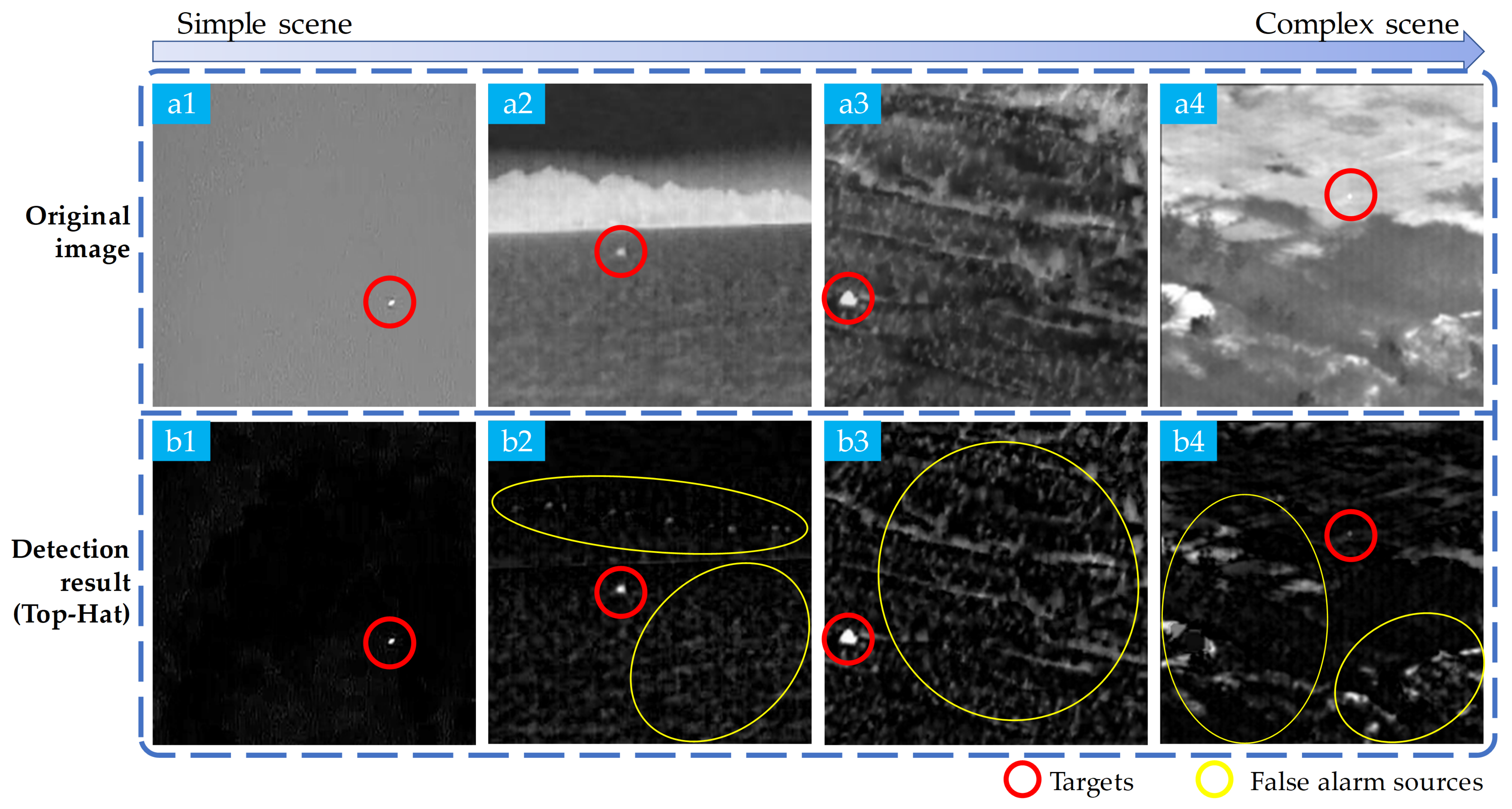
Figure 1. Images (1) to (4) depict four scenes with backgrounds ranging from simple to complex. Row (a) shows the original images; row (b) displays the results processed by the Top-Hat algorithm. It is evident that, as the scenes become more complex, an increasing number of false alarm sources appear, resulting in the targets being less salient.
Remotesensing 16 01758 g001
Figure 2. Architecture of the proposed TFCD-Net consisting of two main stages. In the false alarm suppression stage, multiple FEBs are employed to estimate false alarm sources stepwisely. The false alarm-subtracted result is input into the target segmentation stage to detect the targets. The lower section depicts the FEB.
Remotesensing 16 01758 g002
Figure 3. Overall framework utilizing different connection configurations. The upper section shows the series configuration with 3 FEBs, and the lower section shows the stepped configuration with 3 FEBs. The number of FEBs can be adjusted according to the requirements.
Remotesensing 16 01758 g003
Figure 4. Structural configurations of overall framework used in ablation experiments.
Remotesensing 16 01758 g004
Figure 5. Sample images of NUAA-SIRST dataset.
Remotesensing 16 01758 g005
Figure 6. Sample images of NUDT-SIRST dataset.
Remotesensing 16 01758 g006
Figure 7. The sampling points for each block, indicated by blue arrows.
Remotesensing 16 01758 g007
Figure 8. Inputs and outputs of each block for scene 1.
Remotesensing 16 01758 g008
Figure 9. Three–dimensional visualization of inputs and outputs of each block for scene 1.
Remotesensing 16 01758 g009
Figure 10. Inputs and outputs of each block for scene 2.
Remotesensing 16 01758 g010
Figure 11. Three–dimensional visualization of inputs and outputs of each block for scene 2.
Remotesensing 16 01758 g011
Figure 12. Results and 3D visualizations of different methods for scene 1. The red boxes identify the target area and zoom in for display.
Remotesensing 16 01758 g012
Figure 13. Results and 3D visualizations of different methods for scene 2. The red boxes identify the target area and zoom in for display.
Remotesensing 16 01758 g013
Figure 14. Results and 3D visualizations of different methods for scene 3. The red boxes identify the target area and zoom in for display.
Remotesensing 16 01758 g014
Figure 15. Results and 3D visualizations of different methods for scene 4. The red boxes identify the target area and zoom in for display.
Remotesensing 16 01758 g015
Figure 16. Results and 3D visualizations of different methods for scene 5. The red boxes identify the target area and zoom in for display.
Remotesensing 16 01758 g016
Figure 17. Results and 3D visualizations of different methods for scene 6. The red boxes identify the target area and zoom in for display.
Remotesensing 16 01758 g017
Figure 18. 3D ROC curves with corresponding 2D ROC curves of different methods on NUDT-SIRST dataset. (a) 3D ROC curves. (b) 2D ROC curves of ( P D , P F ) . (c) 2D ROC curves of ( P D , τ ) . (d) 2D ROC curves of ( P F , τ ) .
Remotesensing 16 01758 g018
Figure 19. 3D ROC curves with corresponding two-dimensional ROC curves of different methods on NUAA-SIRST dataset. (a) 3D ROC curves. (b) 2D ROC curves of ( P D , P F ) . (c) 2D ROC curves of ( P D , τ ) . (d) 2D ROC curves of ( P F , τ ) .
Remotesensing 16 01758 g019
Table 1. Ablation results of different structures on 2 datasets.
Structure I o U ( × 10 2 ) NUAA-SIRST
P d ( × 10 2 )
F a ( × 10 6 ) I o U ( × 10 2 ) NUDT-SIRST
P d ( × 10 2 )
F a ( × 10 6 )
A165.4992.0288.978.2390.7941.09
A267.1394.3108.9491.1997.0418.67
A368.6594.30103.5292.6697.4616.63
A466.9593.92104.4592.4397.8817.61
B162.0691.63120.1575.1193.7668.85
B258.8695.06148.9754.3484.34149.49
Table 2. Results achieved on NUDT-SIRST dataset.
Method IoU ( × 10 2 ) Pd ( × 10 2 ) Fa ( × 10 6 ) F 1 ( × 10 2 )
NRAM11.458.5223.4520.47
PSTNN21.6968.04216.6435.65
SRWS8.6966.359.2715.99
ACM67.6595.77138.6680.71
ALCNet69.9394.92118.3182.31
RDIAN86.9397.2534.1993.01
UNet89.8496.419.8994.65
ISTDUNet89.7397.8829.7694.58
DNANet91.6397.4622.7495.63
Proposed92.6697.9917.0196.19
Table 3. Results achieved on NUAA-SIRST dataset.
Method IoU ( × 10 2 ) Pd ( × 10 2 ) Fa ( × 10 6 ) F 1 ( × 10 2 )
NRAM26.1781.7510.2741.49
PSTNN41.6984.7956.5158.84
SRWS12.3684.794.0022.00
ACM63.4992.78113.0877.67
ALCNet64.5293.54117.7978.43
RDIAN70.4693.5495.8982.67
UNet68.2893.1698.3981.15
ISTDUNet66.6692.78104.2479.99
DNANet69.2393.16104.3881.86
Proposed69.3893.1691.8281.92
Table 4. Three-dimensional ROC-derived AUC results achieved on NUDT-SIRST dataset.
Method AUC D , F AUC D , τ AUC F , τ AUC TD AUC BS AUC SNPR AUC TDBS AUC ODP
NRAM0.60670.12090.00500.72760.611824.02640.11590.7226
PSTNN0.75560.28600.00531.04160.760953.70550.28071.0362
SRWS0.62100.10190.00500.72290.626120.29990.09690.7179
ACM0.94060.81610.00511.75660.9457158.69040.81091.7515
ALCNet0.92330.82610.00511.74940.9285161.38910.82101.7443
RDIAN0.97130.93310.00501.90450.9764185.36060.92811.8994
UNet0.96910.92550.00501.89460.9741184.33570.92051.8896
ISTDUNet0.97780.93690.00501.91480.9828186.27000.93191.9097
DNANet0.97570.94830.00501.92400.9807188.81060.94331.9190
Proposed0.97820.95040.00501.92870.9833189.37530.94541.9237
Table 5. Three-dimensional ROC-derived AUC results achieved on NUAA-SIRST dataset.
Method AUC D , F AUC D , τ AUC F , τ AUC TD AUC BS AUC SNPR AUC TDBS AUC ODP
NRAM0.73350.26560.00500.99900.738552.88250.26050.9940
PSTNN0.84060.42270.00511.26320.845782.98560.41761.2581
SRWS0.67090.14290.00500.81390.675928.52920.13790.8089
ACM0.91460.75240.00511.66700.9197147.11860.74731.6619
ALCNet0.90530.77170.00511.67700.9104150.79330.76661.6719
RDIAN0.92270.81710.00511.73980.9278160.33180.81201.7347
UNet0.90920.79510.00511.70430.9143155.94920.79001.6992
ISTDUNet0.91250.78290.00511.69550.9176153.37390.77781.6904
DNANet0.91780.81910.00511.73690.9229160.45840.81401.7318
Proposed0.90980.80560.00511.71540.9151154.00000.80031.7102
Table 6. Comparison of complexity of DNN models on 2 datasets.
MethodParams ( × 10 6 )Inference (ms)Training on NUAA (s/epoch)Training on NUDT (s/epoch)
ACM0.39783.9051.52744.5036
ALCNet0.42703.8941.43354.7769
RDIAN0.21662.7572.60168.2245
UNet34.52592.1164.178713.0852
ISTDUNet2.751913.4896.444618.6608
DNANet4.696615.8198.454026.3606
Proposed1.45014.2033.946312.4757
Disclaimer/Publisher’s Note: The statements, opinions and data contained in all publications are solely those of the individual author(s) and contributor(s) and not of MDPI and/or the editor(s). MDPI and/or the editor(s) disclaim responsibility for any injury to people or property resulting from any ideas, methods, instructions or products referred to in the content.