Article

Effect of the One-to-Many Relationship between the Depth and Spectral Profile on Shallow Water Depth Inversion Based on Sentinel-2 Data

1
Third Institute of Oceanography, Ministry of Natural Resources, Xiamen 361005, China
2
Fujian Provincial Key Laboratory of Marine Physical and Geological Processes, Xiamen 361005, China
3
Observation and Research Station of Coastal Wetland Ecosystem in Beibu Gulf, Ministry of Natural Resources, Beihai 536015, China
*
Author to whom correspondence should be addressed.
Remote Sens. 2024, 16(10), 1759; https://doi.org/10.3390/rs16101759
Submission received: 26 March 2024 / Revised: 9 May 2024 / Accepted: 10 May 2024 / Published: 15 May 2024
(This article belongs to the Special Issue Remote Sensing Applications in Ocean Observation (Second Edition))

Abstract

:
In shallow water, Sentinel-2 multispectral imagery has only four visible bands and limited quantization levels, which easily leads to the occurrence of the same spectral profile but different depth (SSPBDD) phenomenon, resulting in a one-to-many relationship between water depth and spectral profile. Investigating the impact of this relationship on water depth inversion models is the main objective of this paper. The Stumpf model and three machine learning models (Random Forest, Support Vector Machine, and Mixture Density Network) are employed, and the performance of these models is analysed based on the spatial distribution of the training dataset and the input information composition of these models. The results show that the root mean square errors (RMSEs) of the depth inversion of Random Forest and Support Vector Machine are significantly affected by the spatial distribution of the training dataset, while minimal effects are observed for the Stumpf model and the Mixture Density Network model. The SSPBDD phenomenon is widespread in Sentinel-2 images at all depths, particularly between 5 m and 15 m, with most of the depth maximum difference of the SSPBDD pixels ranging from 0 to 5 m. The SSPBDDs phenomenon can significantly reduce the inversion accuracy of any model. The number and the depth maximum difference of the SSPBDDs pixels are the main influencing factors. However, by increasing the visible spectral information and the spatial neighbourhood information in the input layer of machine learning models, the inversion accuracy and stability of the models can be improved to a certain extent. Among the models, the Mixture Density Network achieves the best inversion accuracy and stability.

1. Introduction

Shallow water bathymetry around islands and reefs as well as in nearshore areas is crucial for applications such as navigation safety, engineering construction, resource development, marine rescue, and ecological protection [1]. Satellite remote sensing has the advantages of being free from geospatial constraints and low cost, overcoming the limitations of traditional in situ surveys. Shallow water depth inversion using optical satellites is rapidly developing and gaining attention. There are three types of optical remote sensing depth inversion: active optical, passive optical, and multisource fusion. Three types of depth inversion models exist for passive optical multispectral images: theoretical analytical models, semi-theoretical and semi-empirical models, and statistical models [2]. Statistical models, such as the classical Stumpf dual-band logarithmic ratio algorithm, are widely used due to their relative simplicity and ability to account for local variations in water properties and bottom types. However, they may not achieve the same level of accuracy as theoretical analytical models, which rely on precise knowledge of inherent optical properties, or semi-theoretical and semi-empirical models, which require site-specific calibration. Nevertheless, statistical models offer a more practical approach when accurate inherent optical property data or extensive calibration data are unavailable, making them a viable option for many applications. In recent years, many improved algorithms, such as machine learning models, have emerged that can construct complex nonlinear relationships between multispectral data and bathymetry data, e.g., Random Forest (RF), Support Vector Machine (SVM), and Multilayer Perceptron. These models have improved the accuracy of bathymetry inversion to a certain extent [2]. In recent years, there has been significant progress in the development and application of optical satellite inversion methods with different machine learning algorithms, e.g., using the quasi-analytical algorithm and remote sensing reflectance [3]. In addition to multispectral information, spatial information on bathymetry distributions has been considered in bathymetry inversion models [4,5,6].
However, some characteristics of multispectral satellite sensors are usually ignored; for example, the OLI sensor of Sentinel-2 is not specially designed for water colour remote sensing [7]; there are fewer multispectral bands which are relatively wide, leading to averaging, which mean some spectral information is missing and water body spectra are not depicted in detail. Additionally, Sentinel-2 imagery has limited quantization levels, usually 12 bits, equivalent to 4096 digital numbers [8], which is not sensitive enough for water body bands with smaller intensity variations. Therefore, pixels at different locations and depths maybe have identical spectral profiles, referred to in this paper as the “same spectral profile but different depth (SSPBDD)” phenomenon; a detailed analysis is provided in Section 3.1. This phenomenon is similar to that of “different objects with identical spectrum profiles” in land remote sensing (different types of land cover with identical spectral characteristics) [9,10,11,12]. The most direct impact of this phenomenon is the one-to-many relationship between the depth and spectral profile. For depth inversion models established solely based on spectral characteristics, uncertainty exists in the depth inversion, thus affecting the accuracy of the inversion. Especially for statistical models and machine learning models based on blue–green bands, each input needs to correspond to a unique output, while the impact of the SSPBDD phenomenon that causes one multispectral profile to correspond to multiple different depths (i.e., one-to-many relationship) has not yet been studied.
To address this one-to-many issue, a Mixture Density Network (MDN) is introduced for water depth inversion; MDN is based on machine learning and is compared with the classical Stumpf two-band logarithmic ratio model, the RF model, and the SVM model to study the effect of the SSPBDD phenomenon on the depth inversion accuracy of each model in Section 4 of this paper.

2. Study Area and Data

2.1. Study Area

Kaneohe Bay of Oahu Island, a semi-enclosed harbour that includes a large lagoon and a protected reef system, is located on the northeast side of Oahu Island in the Hawaiian Islands within the United States. The average depth in the bay is 8 m. Fringing reefs are widely distributed along its coastlines, and a large number of patch reefs are found within the lagoon. Outside the lagoon, there is a crescent-shaped reef that is approximately 5 km long and 2 km wide, with a steep reef slope on the seaward side. Kaneohe Bay features a prominent tidal channel that connects the coral reef bay to the open ocean, allowing large volumes of seawater to flow in and out with rising and falling tides.
Buck Island is located on the northeast shallow shelf of the largest island, Saint Croix, in the U.S. Virgin Islands. The southwest coast is mainly composed of exposed sandy beaches. The island is surrounded by reefs from southeast to northwest, forming a lagoon that is 200–300 metres wide and 2–4 metres deep. The outer perimeter is surrounded by numerous isolated patch reefs, and the water surrounding the island is clear. The substrates of the seabeds of these two islands include coral reefs as well as sand and mud [13].

2.2. Data

(1) Satellite data
The satellite images (Figure 1 and Figure 2) used in this study are listed in Table 1, with the Sentinel-2A image overpassed on 29 January 2022 at 14:57 (UTC) and the Sentinel-2B image on 1 December 2020 at 12:23 (UTC). The images of Sentinel-2A and Sentinel-2B were downloaded from the European Space Agency (ESA), and are Level 2A products which have been atmospheric corrected. Since the sun glint is not significant in these two images, to preserve the original information of the data as much as possible, no flare correction was performed in this study. Refer to the methods provided in reference [14] to extract all water body pixels. After the aforementioned processing, the pixel values of the remote sensing images are in terms of remote sensing reflectance (abbreviated as Rrs). To fully utilize the bathymetry information from the various bands of Sentinel-2A and Sentinel-2B, Band 1 (B1) was resampled to a spatial resolution of 10 metres, and the measured depths for Oahu Island and Buck Island were also resampled to a resolution of 10 metres. Furthermore, the tidal heights were obtained from https://tidesandcurrents.noaa.gov/ (accessed on 13 May 2024) based on the position and the acquisition time of the satellite images. Therefore, the tidal height must be subtracted from the inversion depth compared to the measured depth.
(2) Measured depth
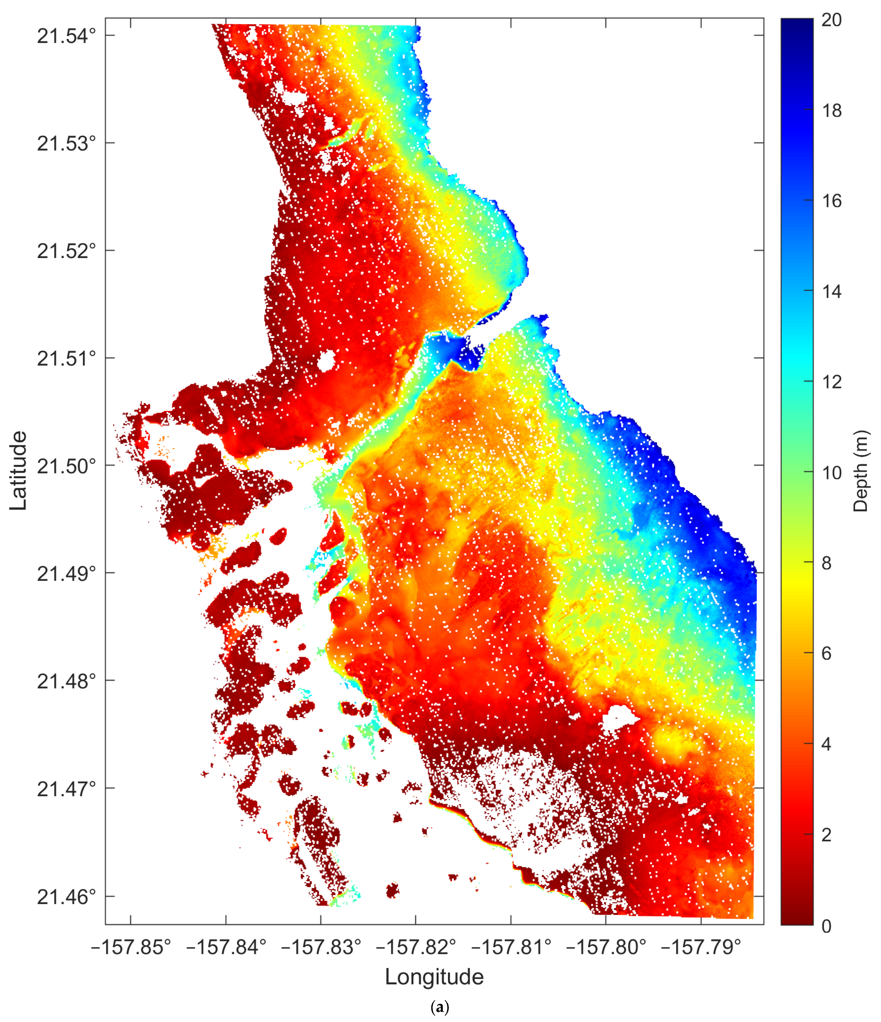
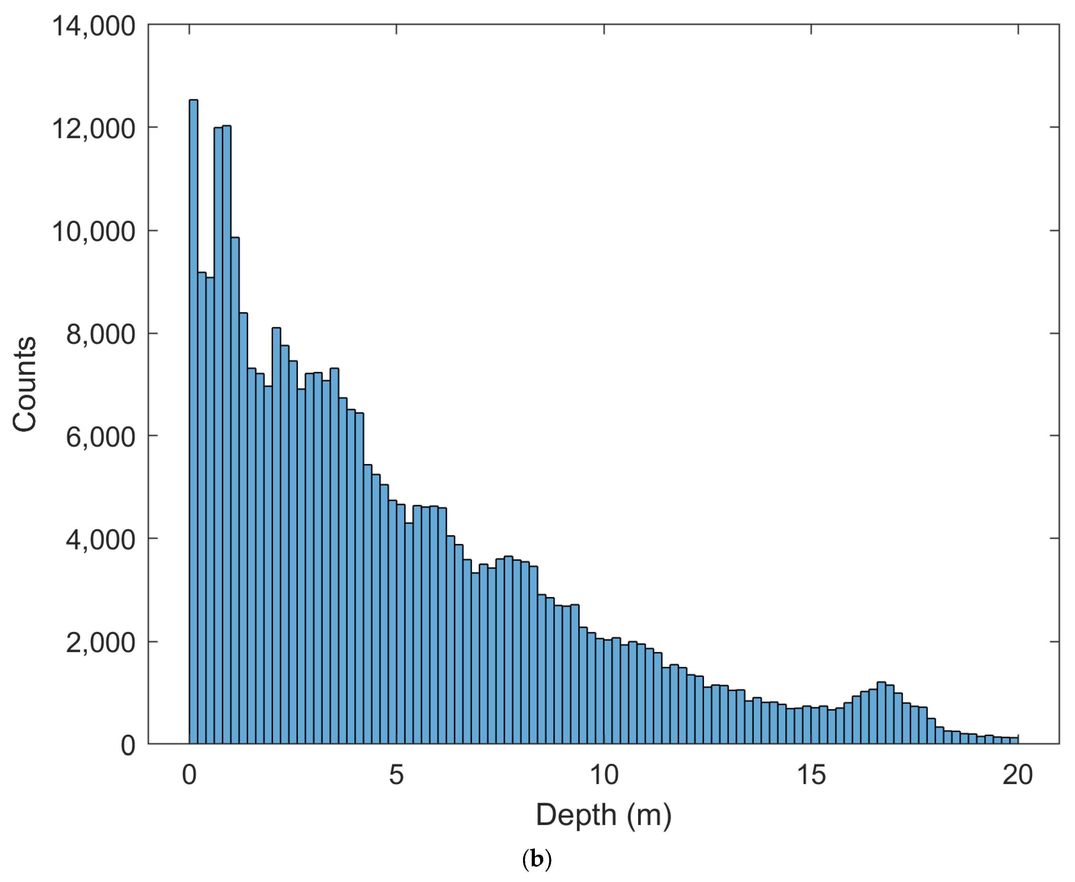
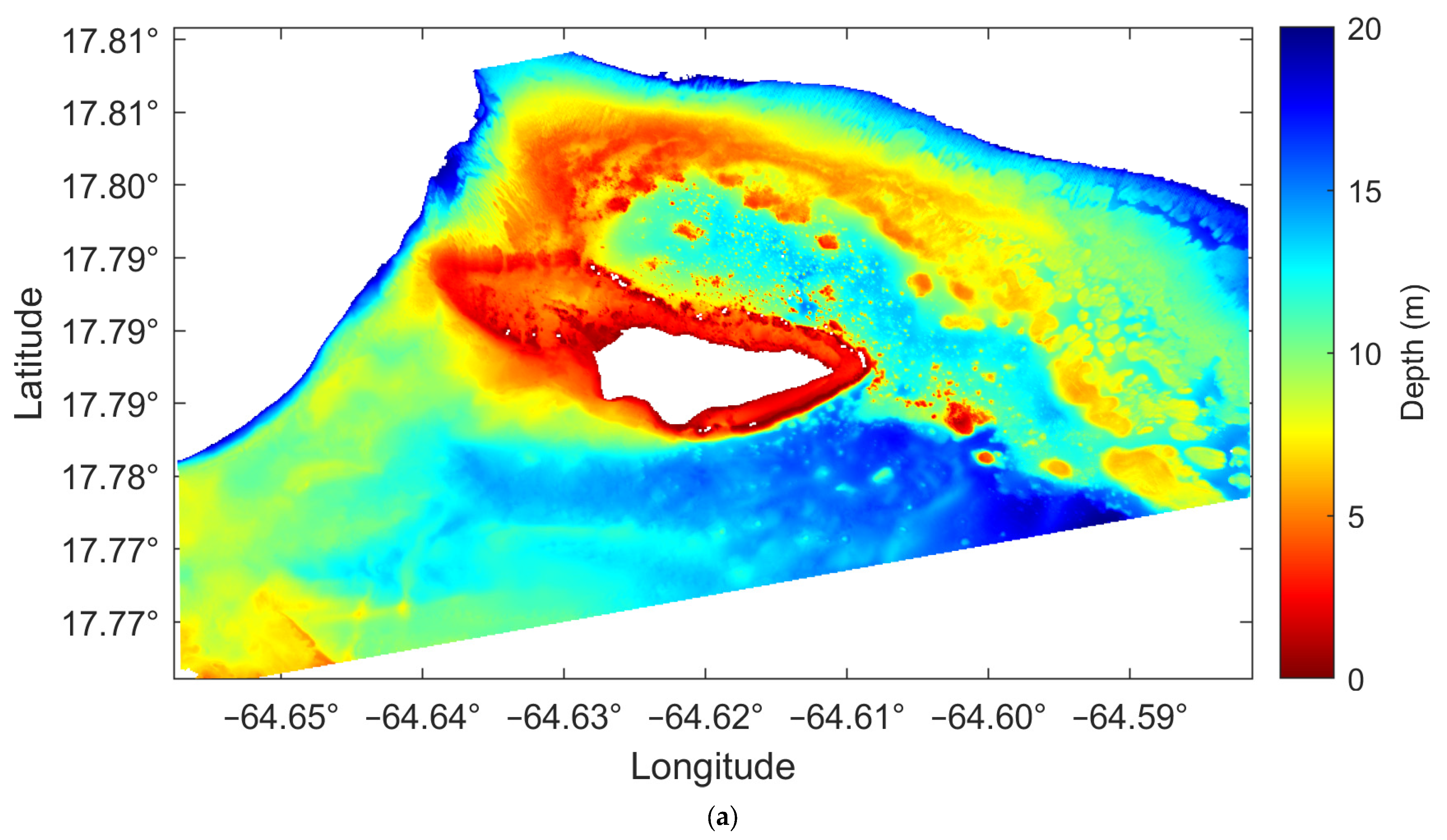
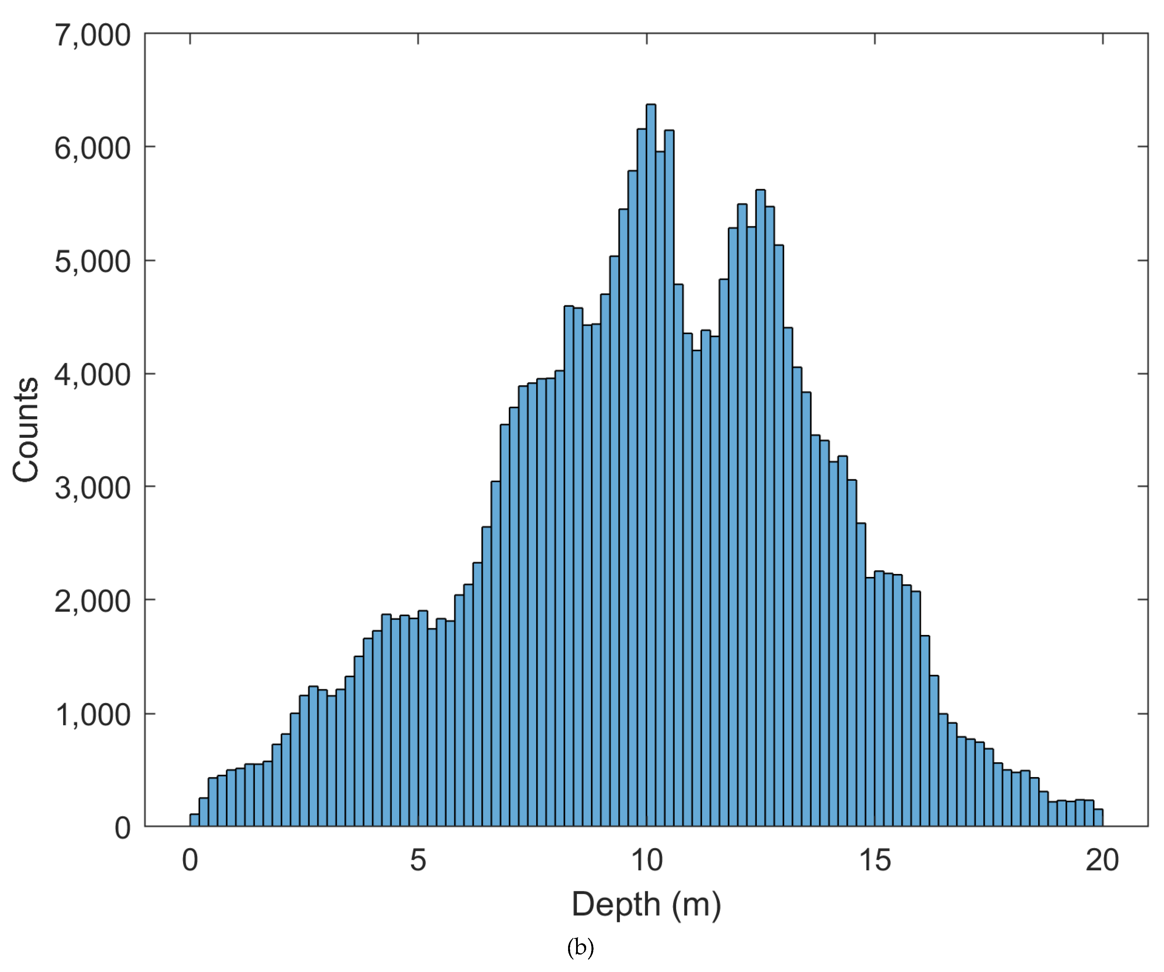
The measured depths used in this study were all derived from airborne LiDAR data obtained from the public dataset of the National Oceanic and Atmospheric Administration (NOAA) Coastal and Ocean Science Centre. The measured depths for Oahu Island (Figure 3a; only 0–20 m depth is shown) consist of irregularly spaced points with an average point spacing of approximately 4 m. The horizontal positioning accuracy is about 3 metres, and the vertical accuracy is about 0.15 m. The measured depths for Buck Island (Figure 4a; only 0–20 m depth is shown) consists of LiDAR points with a spacing of 3 m × 3 m. The vertical and horizontal accuracies of the measured depths meet the requirements of the 1st-order measurement accuracy defined in the 5th edition of the International Hydrographic Organization (IHO) standards [15], with a vertical positioning uncertainty less than [0.52 + (0.013 × depth)2]1/2 metres and a horizontal positioning uncertainty less than (5 + 0.05 × depth) metres. Notably, there are a few scattered blank areas in the measured depths for Buck Island, but this does not affect the overall training or depth inversion. Only water depths within 0–20 m are considered for depth inversion in this paper.
Figure 3b and Figure 4b show the histogram distributions of the measured depths for Oahu Island and Buck Island, respectively. The depth histogram of Oahu Island has a logarithmic shape, with the number of pixels gradually decreasing from shallow water to deep water. On the other hand, the depth histogram of Buck Island looks like a Gaussian shape, with the majority of depths between 9 and 12 m and fewer pixels at depths less than 5 m or greater than 15 m.

3. Methods

3.1. Same Spectral Profile but Different Depth (SSPBDD)

To study the distribution of the SSPBDD phenomenon in the Sentinel-2 images of Oahu Island and Buck Island, the tidal height must be subtracted from the inversion depth to correspond to the spectral profile of each pixel of the Sentinel-2 images. The percentage of pixels with the SSPBDD among the total water pixels (within the depth range of 0–20 m) was calculated under the different band combinations in these two images (Table 2). The percentage of pixels with the SSPBDD is highest for the combination of blue and green bands (B2 and B3), especially for Buck Island, where the SSPBDD phenomenon occurs in almost the entire image. However, when an additional red band (B4) is included, the SSPBDD percentage significantly decreases. When B1 is also included, the SSPBDD percentage is already reduced to a very low level (3.7% for Oahu Island but only 0.7% for Buck Island). Moreover, the addition of B1 leads to a greater decrease in the pixel percentage than does the addition of B4, indicating that B1 provides more spectral information than B4. This is because the transmission of B1 is deeper than that of B4. In any case, increasing the number of visible bands allows for more spectral information about both the water surface and underwater, which is useful to reduce the interference caused by the SSPBDD phenomenon in the one-to-many inversion of depth.
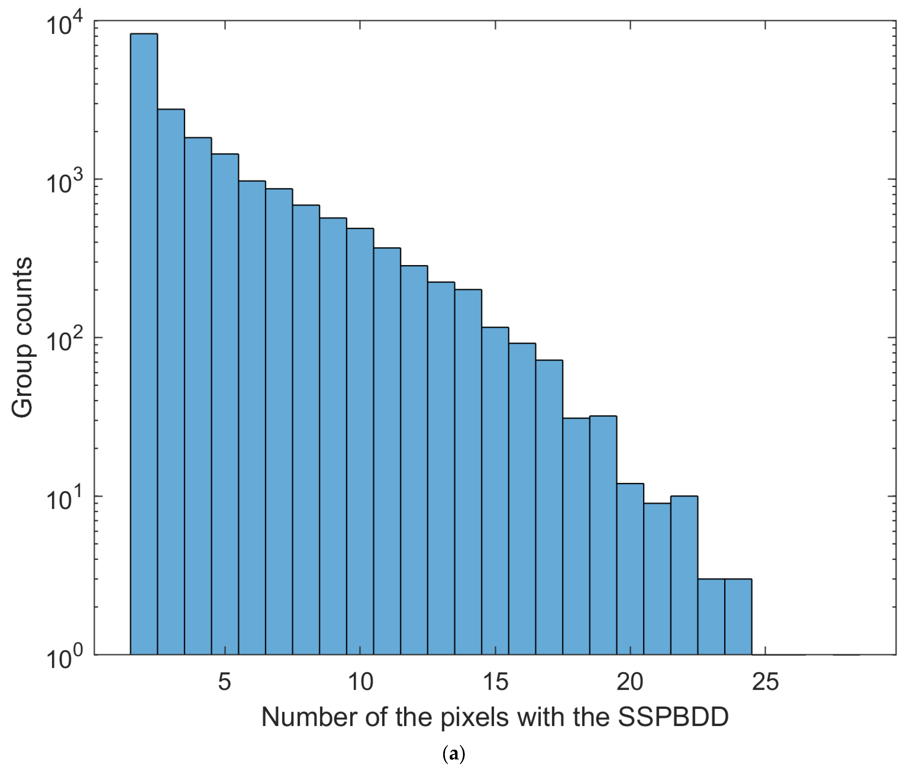
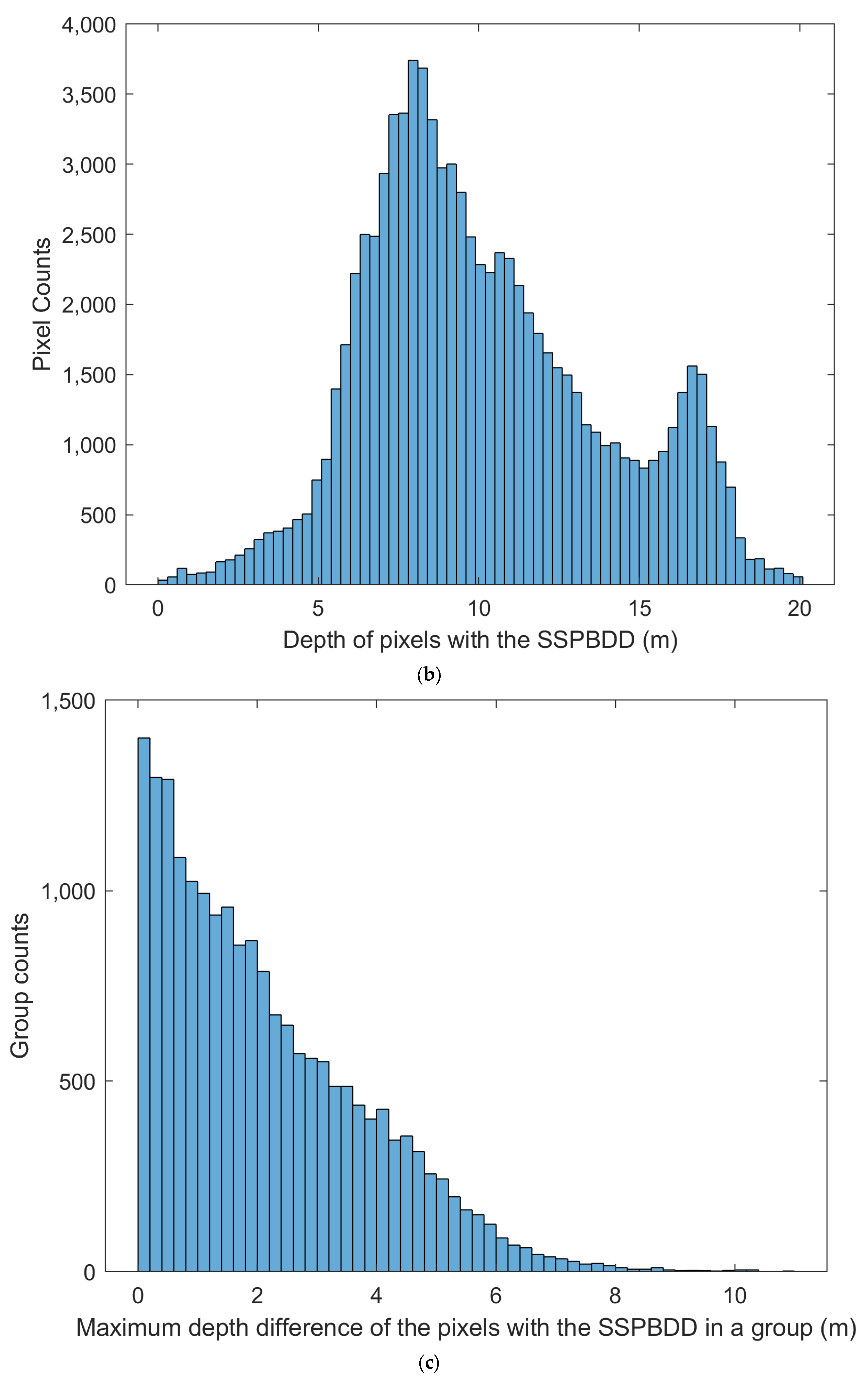
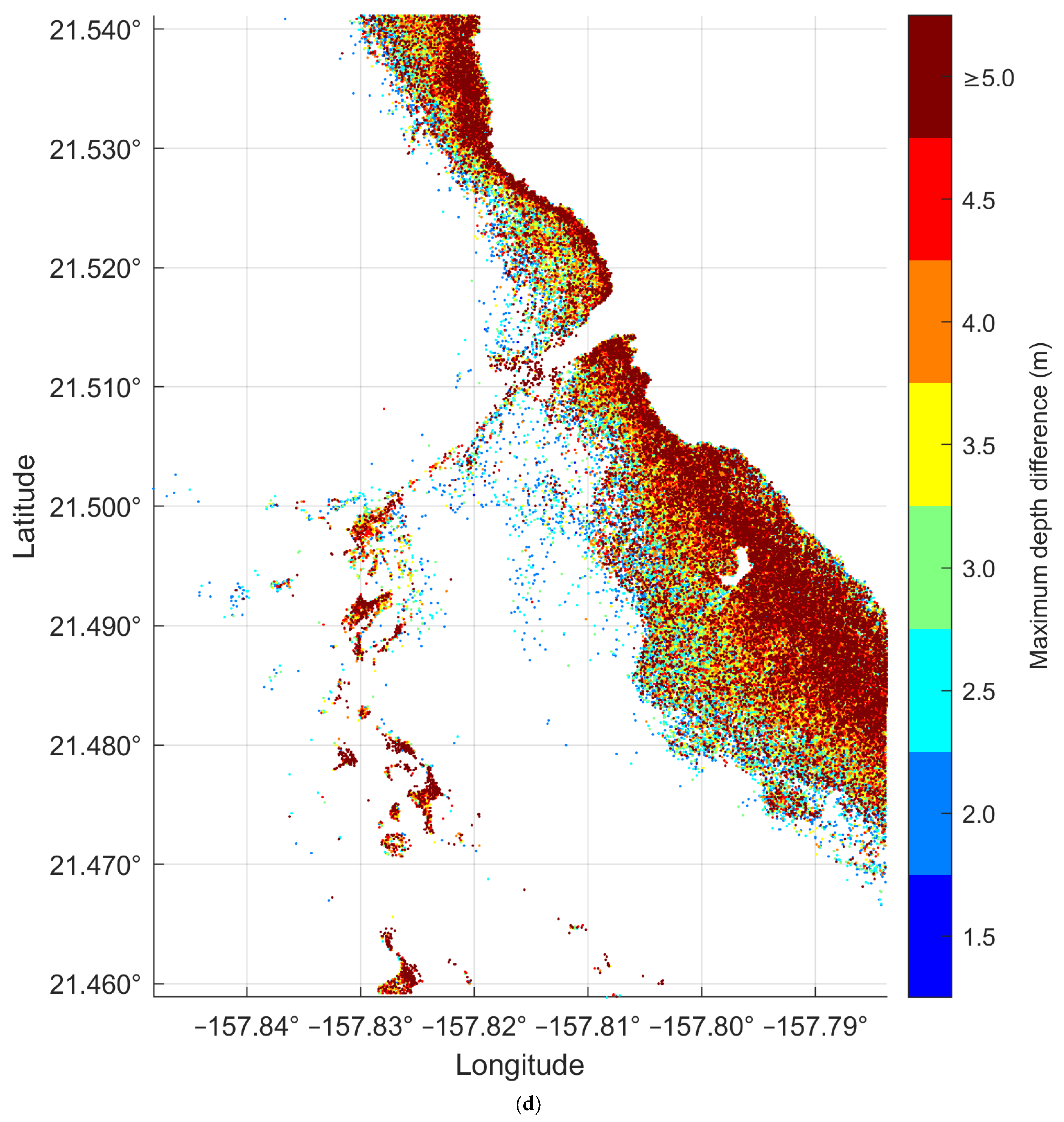
B2, B3, and B4 of Sentinel-2 images are usually used for depth inversion models [16,17,18]. Figure 5 and Figure 6 show the statistics diagram of pixels with the SSPBDD for three-band spectral profiles on Buck Island and Oahu Island, respectively. For example, the value 5 on the X-axis in Figure 5a indicates that the spectral profiles of the 5 pixels in a group are the same; thus, 5 is the number of pixels with the SSPBDD in a group, and the corresponding value 1443 on the Y-axis indicates that there are 1443 groups and there are 5 pixels with the SSPBDD in each group. To study whether those pixels with the SSPBDD are related to water depth, Figure 5b and Figure 6b show histograms of the measured depths corresponding to those pixels. Similarly, the maximum depth difference of pixels with the SSPBDD represents the maximum of difference among water depth among the pixels with the SSPBDD in a group. Figure 5c and Figure 6c show histograms of the maximum depth difference of pixels in each group; then, Figure 5d and Figure 6d show the spatial distribution of those pixels with a maximum depth difference greater than or equal to 1.5 m.
Figure 5a and Figure 6a show the shapes of the histograms for Buck Island and Oahu Island are similar: they both decrease gradually, but the trends are slightly different. For example, there are 1840 groups when 5 pixels have the SSPBDD and only 8 groups when 10 pixels have the SSPBDD on Buck Island; 1443 groups when 5 pixels have the SSPBDD; and 489 groups when 10 pixels have the SSPBDD on Oahu Island. In addition, the maximum number of pixels with the SSPBDD is 11 for Buck Island in one group, while the maximum number of pixels with the SSPBDD reaches 24 for Oahu Island in one group. Table 2 shows that although the percentage is lower on Oahu Island than on Buck Island, the SSPBDD phenomenon is more significant due to a greater number of pixels with the SSPBDD on Oahu Island. The histograms in Figure 5b and Figure 6b both closely resemble a Gaussian shape, which means that the SSPBDD phenomenon mainly occurs at water depths of 5–15 m. In addition, they show that the probability of the SSPBDD phenomenon is relatively low in depths of 0–5 m, possibly because the effect of the seafloor on remote sensing reflectance is more significant at depths of 0–5 m than at other depths, since Figure 3b shows that there are many more pixels at 0–5 m, so this may be the reason why the percentage is lower on Oahu Island than on Buck Island in Table 2, meaning that percentage of pixels with the SSPBDD is related to water depth. Figure 5c and Figure 6c show that the count of groups decreases sharply as the maximum depth difference increases, reaching maximum water depths of 11 m and 13 m, respectively, where only a very small number of groups are present. Figure 5d and Figure 6d show only 65,240 pixels with a depth greater than or equal to 1.5 m and 15,055 pixels with a maximum depth difference greater than or equal to 5 m for Oahu Island, and there are 55,707 pixels with a maximum depth difference greater than or equal to 1.5 m and 1605 pixels with a depth greater than or equal to 5 m for Buck Island. Referring to Figure 3a and Figure 4a, the distributions of these pixels can be summarised as follows: most pixels are in the lagoon areas and at 5–15 m depth on the two islands, in the tidal channel on Oahu Island, and near the image boundary on Buck Island.
In conclusion, Figure 5 and Figure 6 show that the SSPBDD is a common phenomenon in data from the multispectral satellite Sentinel-2, and the spatial distribution of pixels with the SSPBDD is significantly correlated with the water depth, and the difference between the water depth corresponding to pixels with the SSPBDD is also relatively obvious, so it is necessary to study the effect of the SSPBDD on the depth inversion.

3.2. Parameters

3.2.1. Depth Invariant Index (DII)

Lyzenga proposed a method to extract substrate types by using the DII because sunlight decays exponentially in the water column with depth [19]. The DII is defined in this paper as follows:
D I I = l n R B 2 k B 2 / k B 3 l n R B 3
where R B 2 and R B 3 are the reflectance at B 2 and B 3 , respectively. k B 2 and k B 3 are the attenuation coefficients of the water column at B 2 and B 3 , respectively. The entire shallow sea around Oahu Island and Buck Island is clear, and the marine environment is minimally affected by human activities; therefore, a homogeneous water column is assumed. Based on this assumption, the attenuation coefficient ratio k B 2 / k B 3 will be a constant [20]. k B 2 / k B 3 = 0.68 was set for this paper.

3.2.2. Spatial Neighbourhood Parameters

From the perspective of the spectral dimension, DII is just a nonlinear expression of satellite bands, which can be considered as redundant spectral information for pixels with the same spectral profile, which cannot change the one-to-many relationship caused by the SSPBDD. The latitude and longitude [4,21,22] of the pixel and satellite image patches [5,23] are used as input information for training the depth inversion model and the accuracy of depth inversion is improved, which proves that the spatial dimension of the satellite image is also necessary information for the depth inversion. However, the spatial information used in this paper is different from that used in the methods of those papers, because the bathymetric information should not be related to the absolute spatial position between the surrounding adjacent pixels, but only to the relative positions of the surrounding adjacent pixels and the distributions of the depth and spectral profiles, which is referred to as spatial neighbourhood information. In this paper, the mean and the standard deviation of a 5 × 5 moving window of B1, B2, B3, and B4 are used as the representation parameters of the neighbourhood information; for situations where pixels are in the image boundary or contain non-water pixels in the 5 × 5 moving window, the mean and the standard deviation are calculated only for water body pixels.

3.3. Depth Inversion Models

3.3.1. Stumpf Model

Stumpf [24] proposed a dual-band logarithmic ratio empirical model that links the logarithmic ratio of the remote sensing reflectance of two visible light bands with the bathymetric data through a linear relationship. This model, which has been applied widely to shallow bathymetric water and achieved good results [1,25], is given as follows:
z = m 1 ln ( n r r s ( B 2 ) ) ln ( n r r s ( B 3 ) ) m 0
where m1 is a slope constant, m0 is the offset of the logarithmic ratio when the bathymetric z is 0 metres, and n is a fixed constant, which ensure that the logarithmic value is positive in all cases and that the logarithmic ratio has a linear relationship with the depth z. m0 and m1 can be obtained by least squares linear regression using training data.

3.3.2. Random Forest (RF) Model

The RF model and SVM model are common machine learning algorithms that are widely used for satellite-derived bathymetry [26]. RF regression is an ensemble technique that reduces variance and overfitting to individual trees through bootstrap aggregation or bagging and integrates predictions from many decision trees to improve accuracy and stability [27]. In this paper, the parameters of the RF model were set such that the number of decision trees was 300 and the minimum number of leaf node observations was five.

3.3.3. Support Vector Machine (SVM) Model

SVM is a supervised learning method for complex nonlinear regression tasks and was introduced as an extension of SVM classification using epsilon-insensitive loss functions to handle regression, capturing nonlinear relationships between observed spectral bands and depth [28]. The parameters of the SVM model were set such that the Gauss kernel function was used, and automatic hyperparameter optimisation was used for the hyperparameters, reducing cross-validation losses by a factor of five.

3.3.4. Mixture Density Network (MDN) Model

As shown by the Fourier transform, a complex signal can be obtained by combining multiple sinusoidal or cosine signals of different frequencies. Similarly, a complex probability distribution can be obtained by combining multiple simple probability distributions. If the multispectral signal corresponding to a pixel is not a depth but rather a probability distribution of depth, the one-to-many mapping problem of depth-multispectral data can be solved. This method, that is, the mixed density network, was first proposed by Christopher Bishop in the 1990s [29]. Through it, the prediction output of the neural network is no longer a single value but rather the weighted sum of multiple Gaussian distributions with different means and variances.
P y x = k K 1 α k x ϕ y , μ k x , σ k x
where the weight coefficients α k x , mean value μ k x , and variance value σ k x are generated by the training dataset and k K 1 α k x = 1 , σ k x > 0 . The loss function uses the maximum likelihood function of the joint probability distribution.
C o s t F u n c y x = l o g k K 1 α k x ϕ y , μ k x , σ k x  
The e input layer is a normalized remote sensing reflectance.
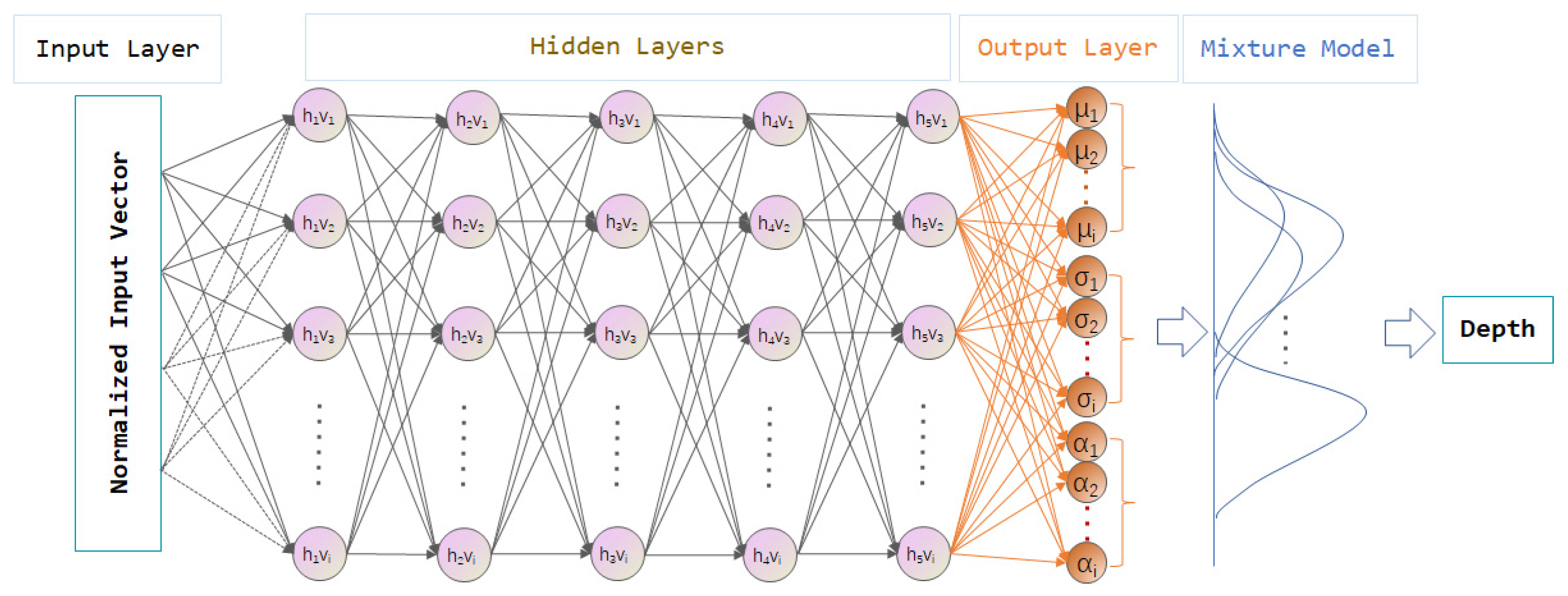
MDN has been used to estimate ocean parameters from multispectral satellite images, such as water quality [30], sea surface wind [31], etc., especially chlorophyll concentration [32,33]. The MDN provides accurate estimates and quantifies prediction uncertainty [34,35]. This demonstrates the potential of MDN to handle the complex nonlinear mapping between oceanic parameters and reflectance. The structure of the fully connected MDN used in this article is shown in Figure 7. After referencing source codes [36] and research results of previous studies, the MDN hyperparameters in this paper were set as follows: 5 hidden layers, each with 100 nodes, and an output layer consisting of 100 weight coefficients, 100 means, and 100 variances, for a total of 300 parameters. These 100 groups of different Gaussian distribution parameters were weighted and superimposed to form a complex probability distribution model. After 50 samplings, according to the input multispectral curve, the median value was used as the inversion depth.

3.4. Training and Evaluation of the Models

Four models (Stumpf, RF, SVM, MDN) are used in this paper. The Stumpf model uses only the blue–green band (B2 and B3) as the input-layer vector, while the RF, SVM, and MDN models use the three bands (Equations (5) and (7)) and four bands (Equations (6) and (8)) from Table 2 as the input-layer vectors; that is,
X 1 = B 2 , B 3 , B 4
X 2 = B 1 , B 2 , B 3 , B 4
Due to the one-to-many issue caused by the SSPBDD, using additional spatial information to reduce the percentage is one of the solutions. The input layer was improved by adding the mean and standard deviation of a 5 × 5 moving window in each band as the input-layer vector; that is,
X 3 = B 1 , B 2 , B 3 , ln ( n r r s ( B 2 ) ) ln ( n r r s ( B 3 ) ) , D I I , m e a n B 2 , m e a n B 3 , m e a n B 4 , s t d B 2 , s t d B 3 , s t d B 4
X 4 = B 1 , B 2 , B 3 , ln ( n r r s ( B 2 ) ) ln ( n r r s ( B 3 ) ) , D I I , m e a n B 1 , m e a n B 2 , m e a n B 3 , m e a n B 4 , s t d B 1 , s t d B 2 , s t d B 3 , s t d B 4
where X 3 and X 4 correspond to the three-band neighbourhood method and the four-band neighbourhood method, respectively, with an enhanced input-layer vector. Since changes in the dual-band logarithmic ratio due to depth are significantly larger than those due to seafloor substrate type, and DII can be used to some extent as an indicator of substrate type [19,37], ln ( n r r s ( B 2 ) ) ln ( n r r s ( B 3 ) ) and D I I are also added to the input-layer vector to improve the accuracy of the depth inversion model as much as possible.
The number of sample points in the training dataset affects the prediction accuracy of the model. Following the results in the literature [24], 3500 random points were chosen as the training dataset. To minimise the instability of the results due to the spatial distribution of random points, all four models were trained ten times with non-repeat datasets of the random points, i.e., each model has ten inversion depths for each pixel. All four models were trained with the same random points each time. The absolute error and the root mean square error (RMSE) were used to evaluate the performance of each model, thereby demonstrating the accuracy of the depth inversion of the different models. The calculation formulas are as follows:
Δ D = D r D m
R M S E = i = 1 n Δ D i 2 n
where Δ D is the absolute error, D r is the inversion depth of the pixel, D m is the measured depth corresponding to the pixel, and RMSE represents the root mean square error of the inversion depth for all pixels each time.

4. Results

4.1. RMSEs of Different Models

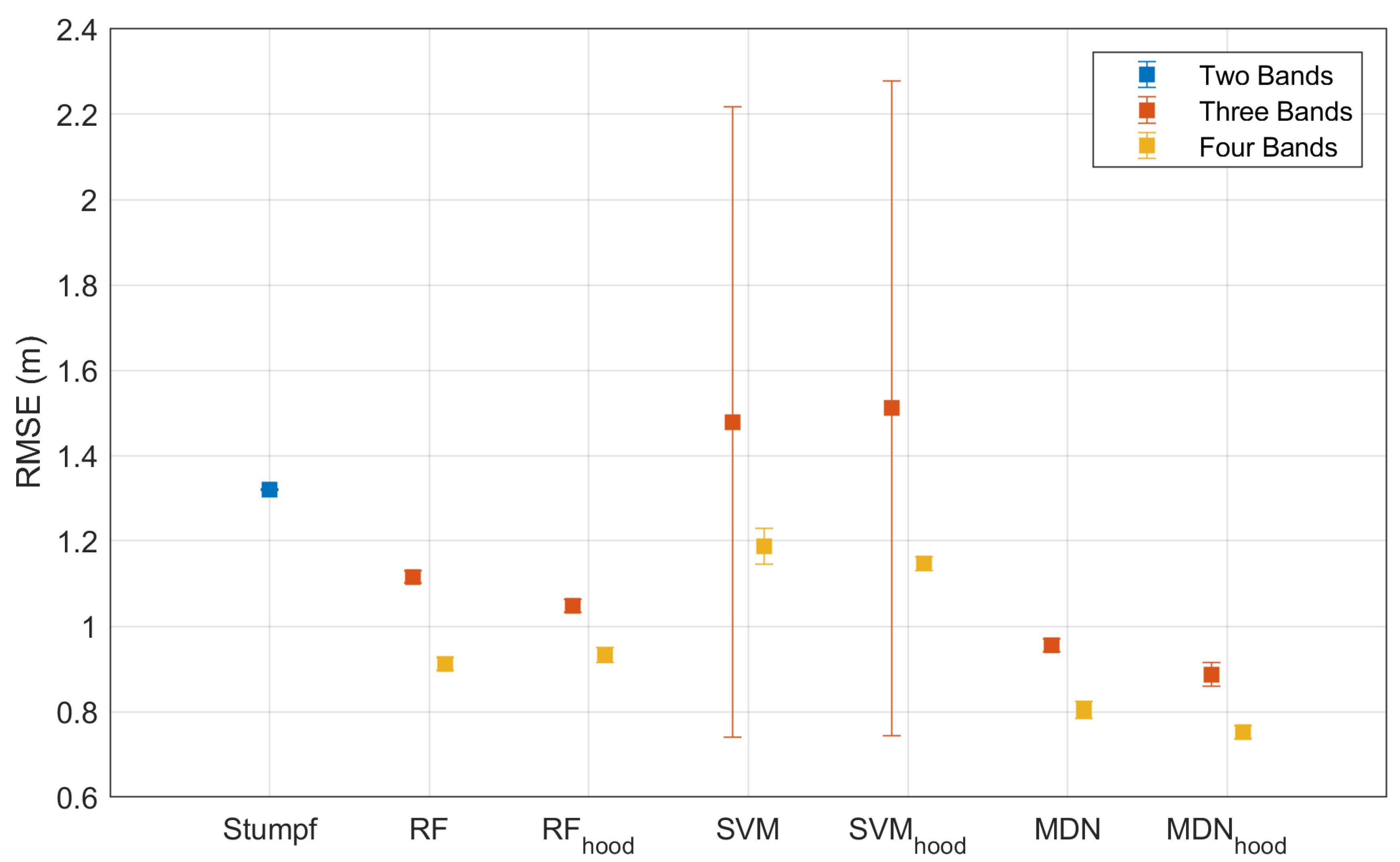
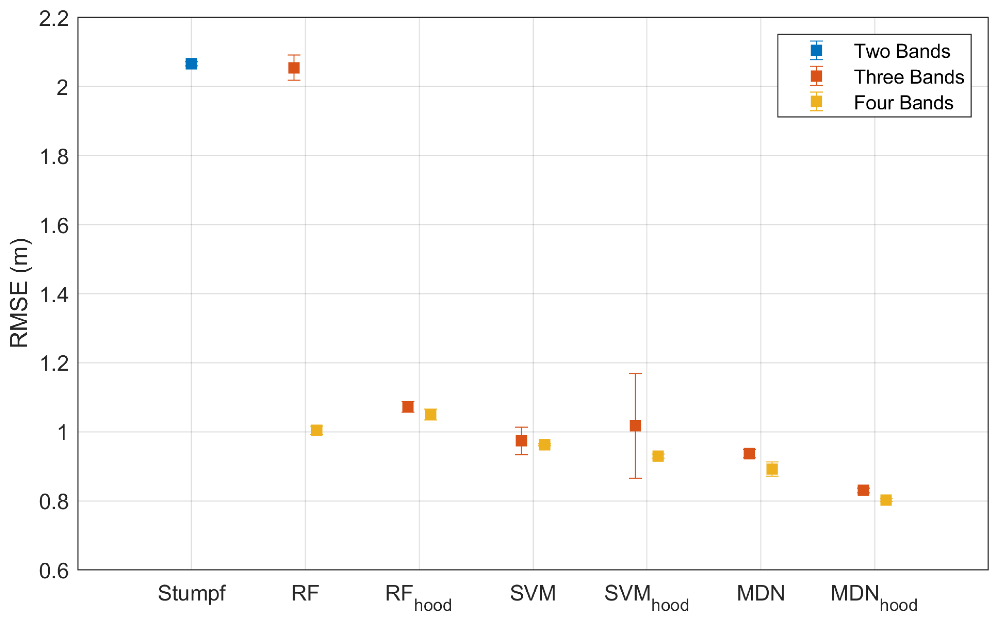
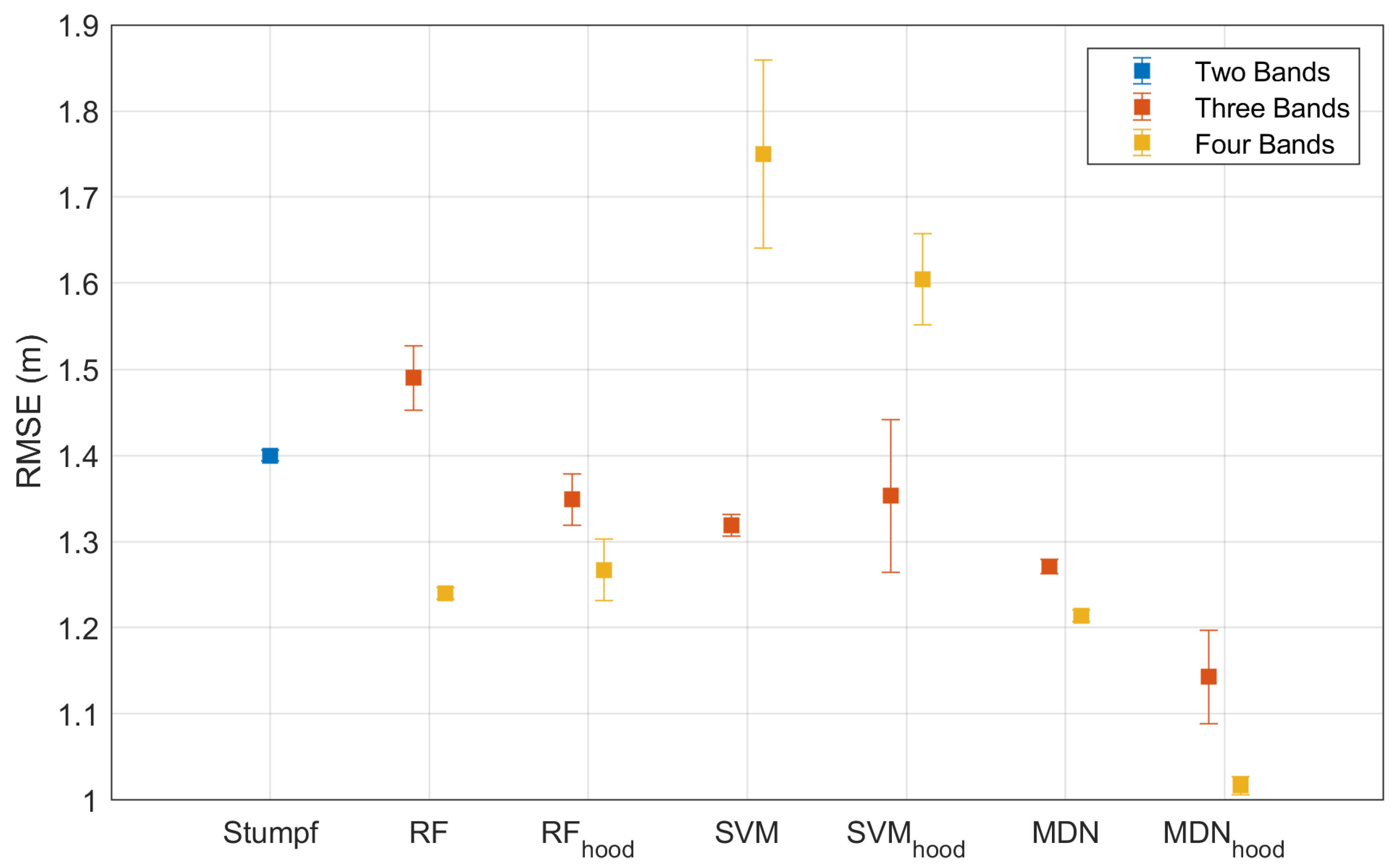
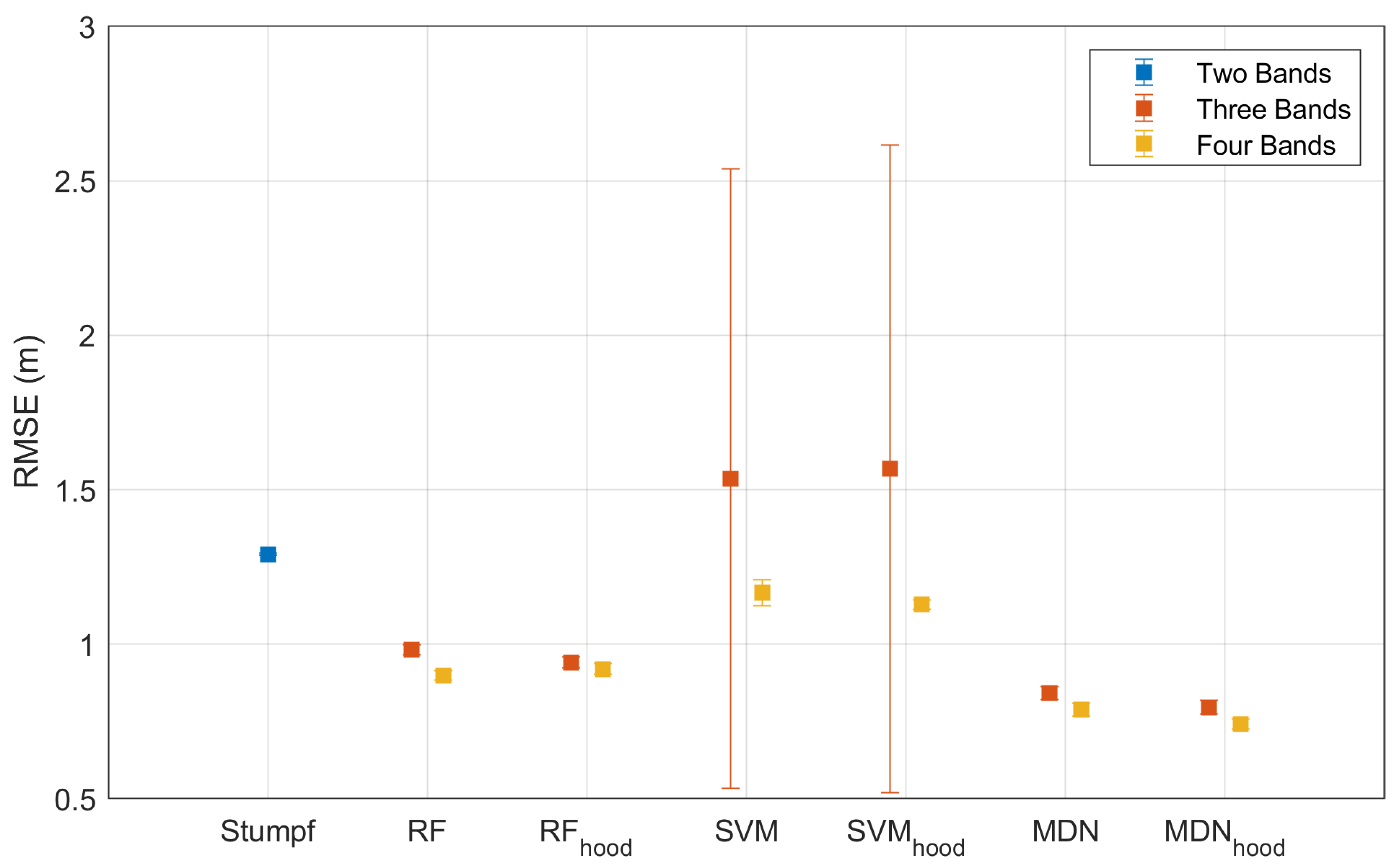
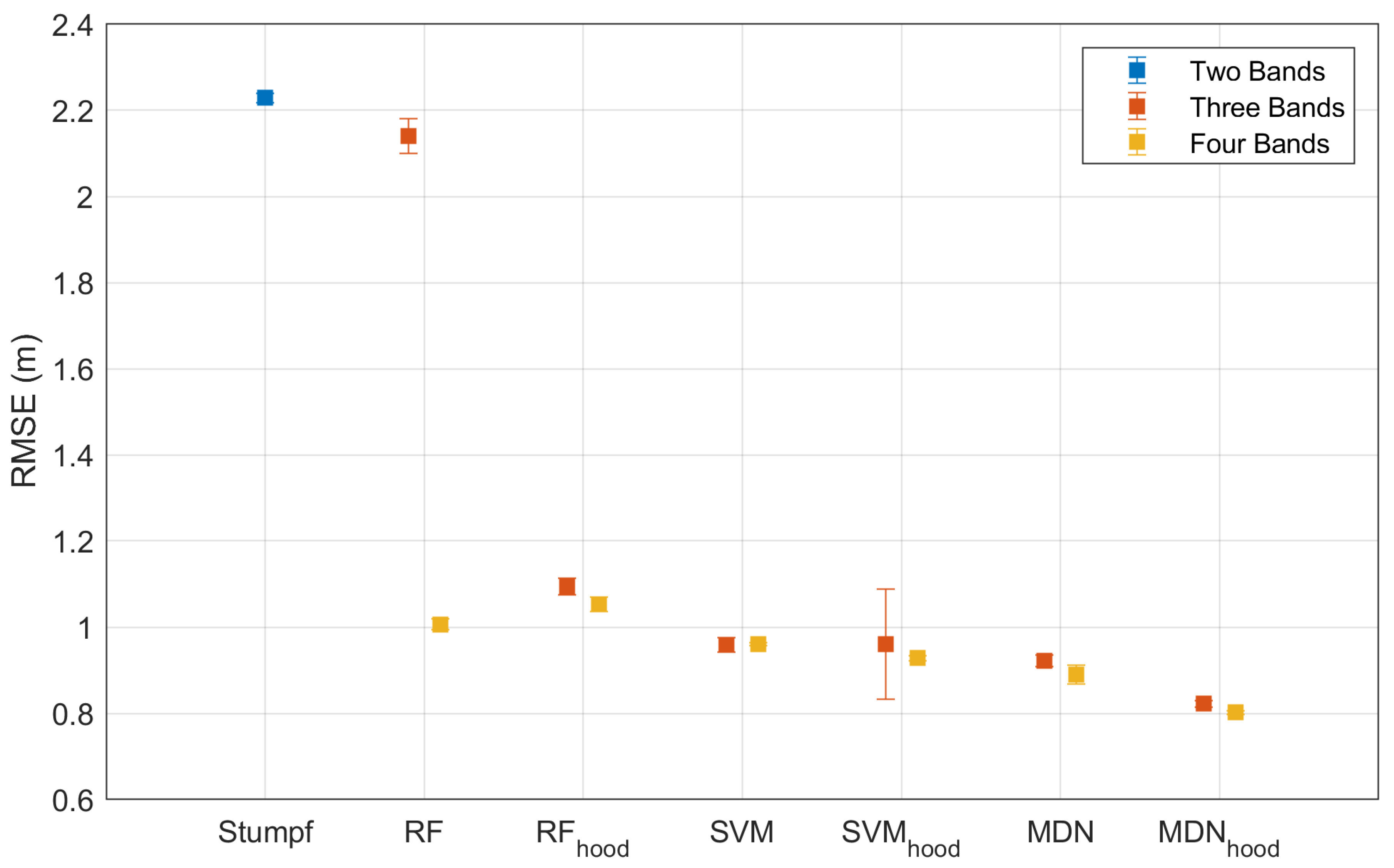
Since each random sampling results in a training dataset with a different spatial distribution of random points, an error bar is used to illustrate the variation in RMSE caused by ten random samplings, which is calculated by the standard deviation of ten RMSEs, representing the uncertainty due to distinct spatial distributions of training datasets. Figure 8 shows the statistical results of RMSE of the depth inversion models (Stumpf, RF, SVM, and MDN) for Oahu Island. The Stumpf model (blue) uses only blue–green bands (B2 and B3), while the other models use three bands (Equations (5) or (7), red) or four bands (Equations (6) or (8), yellow). The subscript “hood” in the model’s name indicates that the input-layer vector of the models is Equation (7) (three-band neighbourhood; red) or Equation (8) (four-band neighbourhood; yellow). The different lengths of the error bars indicate the degree of dispersion of the RMSE distribution, which represents the impact of different training datasets on the results of the depth inversion. Similarly, Figure 9 shows results for Buck Island, while Figure 10, Figure 11, Figure 12 and Figure 13 show results for SSPBDD and non-SSPBDD pixels for Oahu Island and Buck Island, respectively.
Stumpf model: The mean RMSE of the Stumpf model is larger, while the standard deviations of the RMSE are small. This indicates that the inversion accuracy of the Stumpf model is low and that the spatial distribution of the training dataset has little effect on the inversion accuracy of this model. The RMSEs for Buck Island (Figure 10 and Figure 12) are larger than those for Oahu Island (Figure 11 and Figure 13), which may be caused by the SSPBDD phenomenon (Table 2). The percentage of total pixels with the SSPBDD reaches 92.7% for Buck Island, which is much higher than the 37.9% for Oahu Island. The one-to-many features caused by the SSPBDD phenomenon increase the uncertainty of water depth inversion. The RMSE of the pixels with SSPBDD (Figure 10) for Oahu Island is slightly greater than that for non-SSPBDD (Figure 12), while the RMSE of the pixels with SSPBDD (Figure 11) for Buck Island is lower than that for non-SSPBDD (Figure 13). This result can be explained by the fact that the lower percentage of SSPBDD for Oahu Island leads to an insignificant increase in the RMSE, while the higher percentage of the SSPBDD for Buck Island makes the percentage of non-SSPBDD in the training dataset very small, thus resulting in a greater RMSE for the pixels with non-SSPBDD.
RF model: For the three-band RF model, the RMSE of pixels with the SSPBDD is greater than the two-band Stumpf model, while the RMSE with non-SSPBDD is lower than the two-band Stumpf model, indicating that the SSPBDD phenomenon has a greater impact on the three-band RF model. The three-band RF model has relatively longer error bars, meaning that the model is influenced by the spatial distribution of the training dataset to some extent. The RMSEs and error bars are both reduced with the four-band RF model, and the mean RMSE is lower than that of the Stumpf model, demonstrating that adding the B1 band can effectively improve the accuracy and stability of the RF model.
SVM model: For Oahu Island (the four-band model in Figure 10 and the three-band model in Figure 12), the accuracy (mean RMSE) and stability (standard deviation of RMSE) of the SVM model are even worse than those of the Stumpf model; this may be caused by insufficient training for the SVM. According to the literature [35], the required training data size may vary with satellite image. The RMSEs of the SVM model in Figure 11 and Figure 13 demonstrate that adding the B1 band can improve the accuracy and stability of the model.
MDN model: For both Oahu Island and Buck Island, the four-band MDN model outperforms the three-band MDN model, demonstrating that adding the B1 band can significantly improve the accuracy of water depth inversion models. The inversion accuracy with the non-SSPBDD is better than that with the SSPBDD for both island zones, indicating a decrease in the model accuracy due to the existence of the SSPBDD phenomenon. Among the four models, the MDN model achieves the optimal results (mean and standard deviation of the RMSE), indicating that this model is the least affected by the SSPBDD phenomenon and has the lowest requirement for the spatial distribution of the training dataset.
Although the three-band percentage for Oahu Island is lower than that for Buck Island, as shown in Table 2, the four-band percentage for Oahu Island is higher than that for Buck Island. However, in Figure 10, for most of the models the RMSE is larger than that in Figure 11, regardless of the three-band or four-band models. The reasons can be found in Figure 5 and Figure 6. For example, in Figure 5a and Figure 6a, the number of groups with more than seven pixels with the SSPBDD is much greater for Oahu Island than for Buck Island, and only Oahu Island has groups with more than seven pixels. Secondly, in Figure 5c and Figure 6c, the number of pixels with a maximum depth difference larger than 4 m is much greater for Oahu Island than for Buck Island. Since the maximum depth difference represents the difference in water depth between pixels and the SSPBDD phenomenon, a larger maximum depth difference maybe lead to greater inversion errors.
The dual-band logarithmic ratio and DII may be useful to improve the accuracy of the water depth inversion for the non-SSPBDD pixels, but both parameters still belong to the redundant spectral information and cannot change the one-to-many relationship for the SSPBDD pixels. Thus, the improvement in inversion accuracy can be attributed to the spatial information in the input-layer vector for the SSPBDD pixels.
Figure 10, Figure 11, Figure 12 and Figure 13 show that after adding spectral dimension and spatial dimension information, the accuracy of the three-band RFhood model improves the most, especially for Buck Island, as well as for the four-band SVMhood model. However, for the four-band RFhood model and the three-band SVMhood model, the inversion accuracy becomes worse. Regardless, for the MDNhood model, the RMSE is the lowest for both Oahu Island and Buck Island, indicating that the MDNhood model fully exploits the spatial information, which can significantly improve the accuracy of the depth inversion.

4.2. Inversion Results of the Four-Band MDNhood Model

Due to the excellent performance of the four-band MDNhood model, only the inversion results of this model will be analysed in the following.
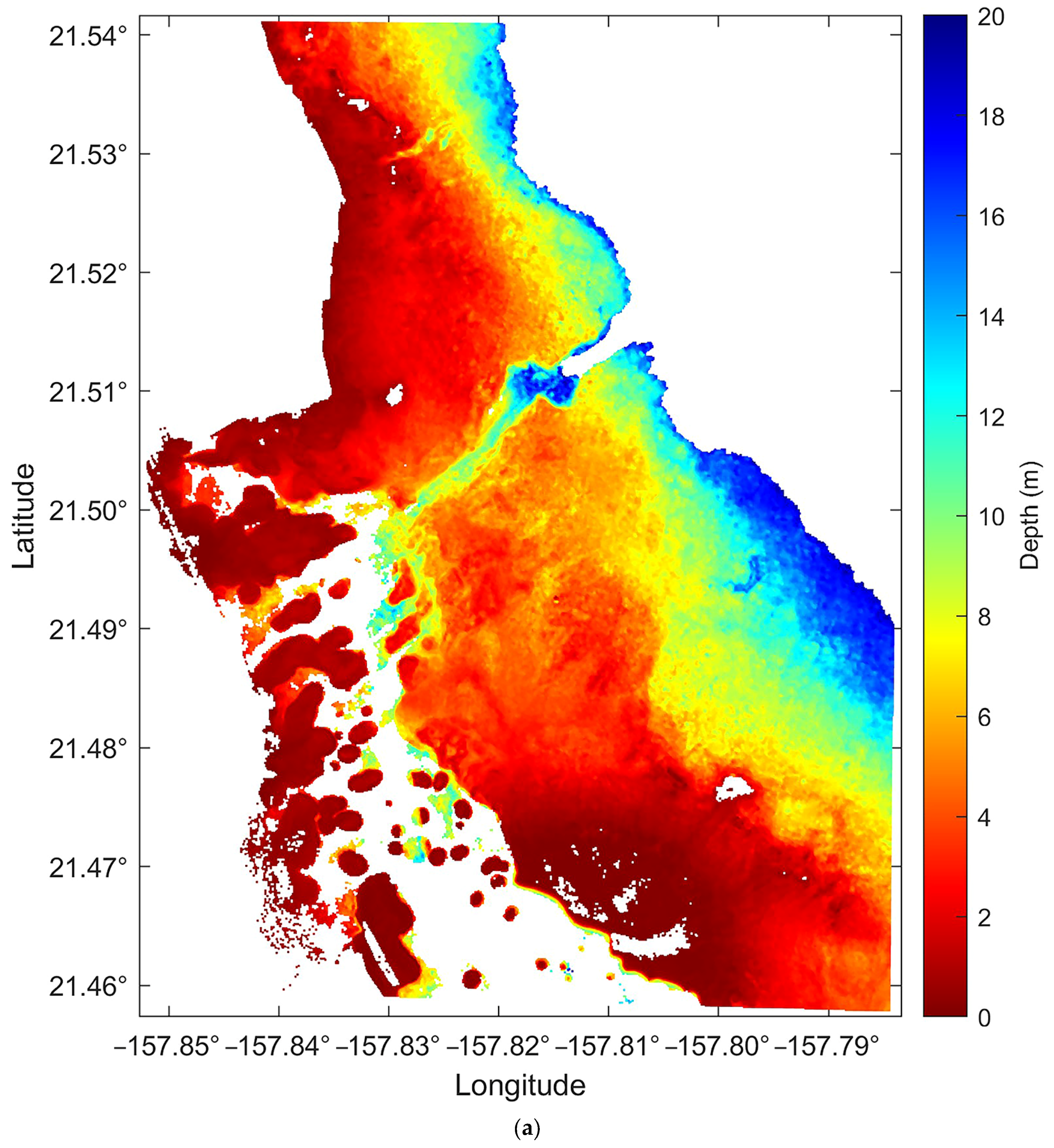
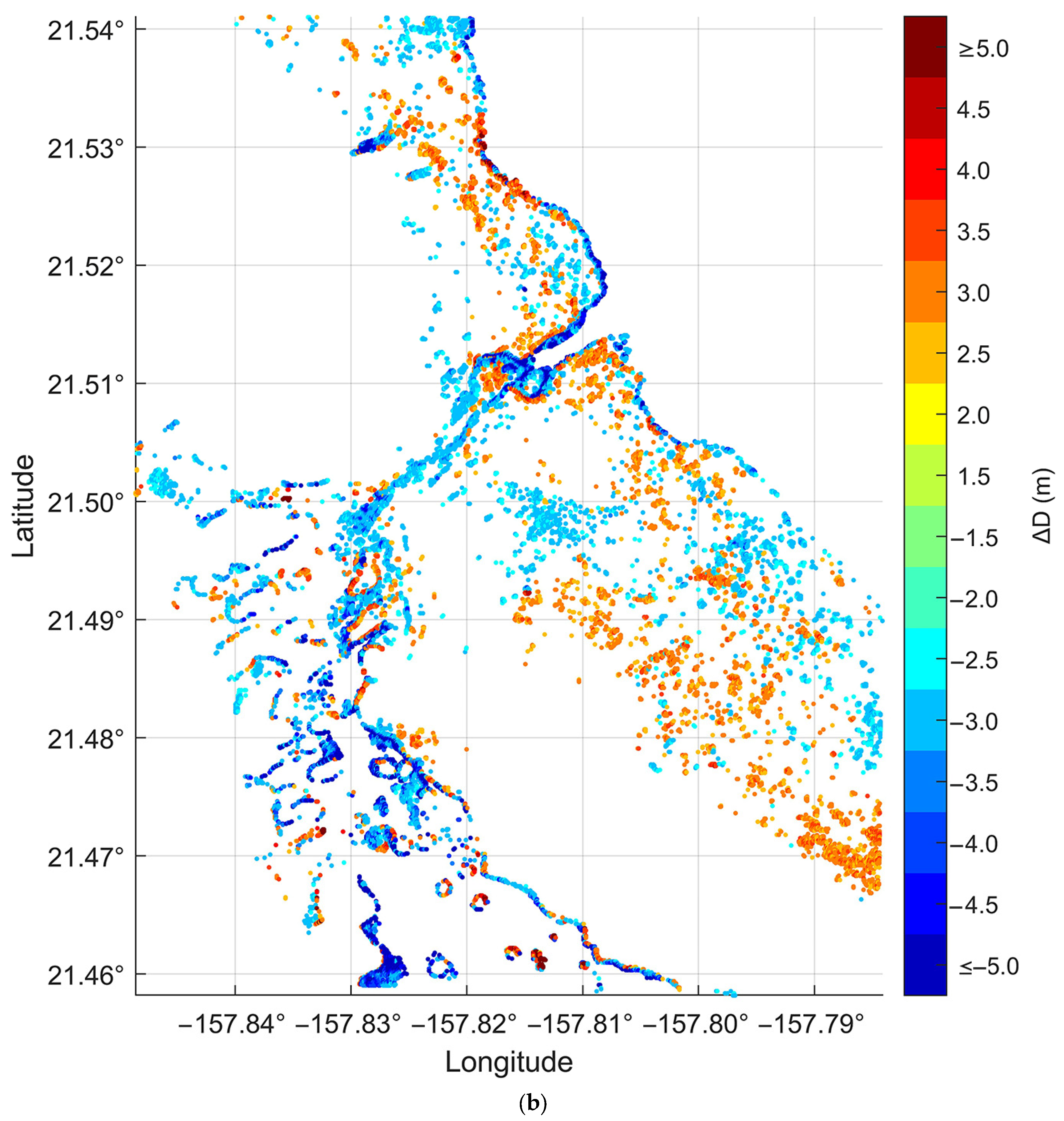
Figure 14 and Figure 15 show the spatial distributions of the water depth and its absolute error |∆D| ≥ 1.5 m for Oahu Island and Buck Island, respectively. Comparing them with the measured depths (Figure 3 and Figure 4), the consistency is noticeable, and the larger value of the absolute error |∆D| mainly occurs in areas with rapid depth changes, such as the lagoon areas, especially the tidal channels on Oahu Island.
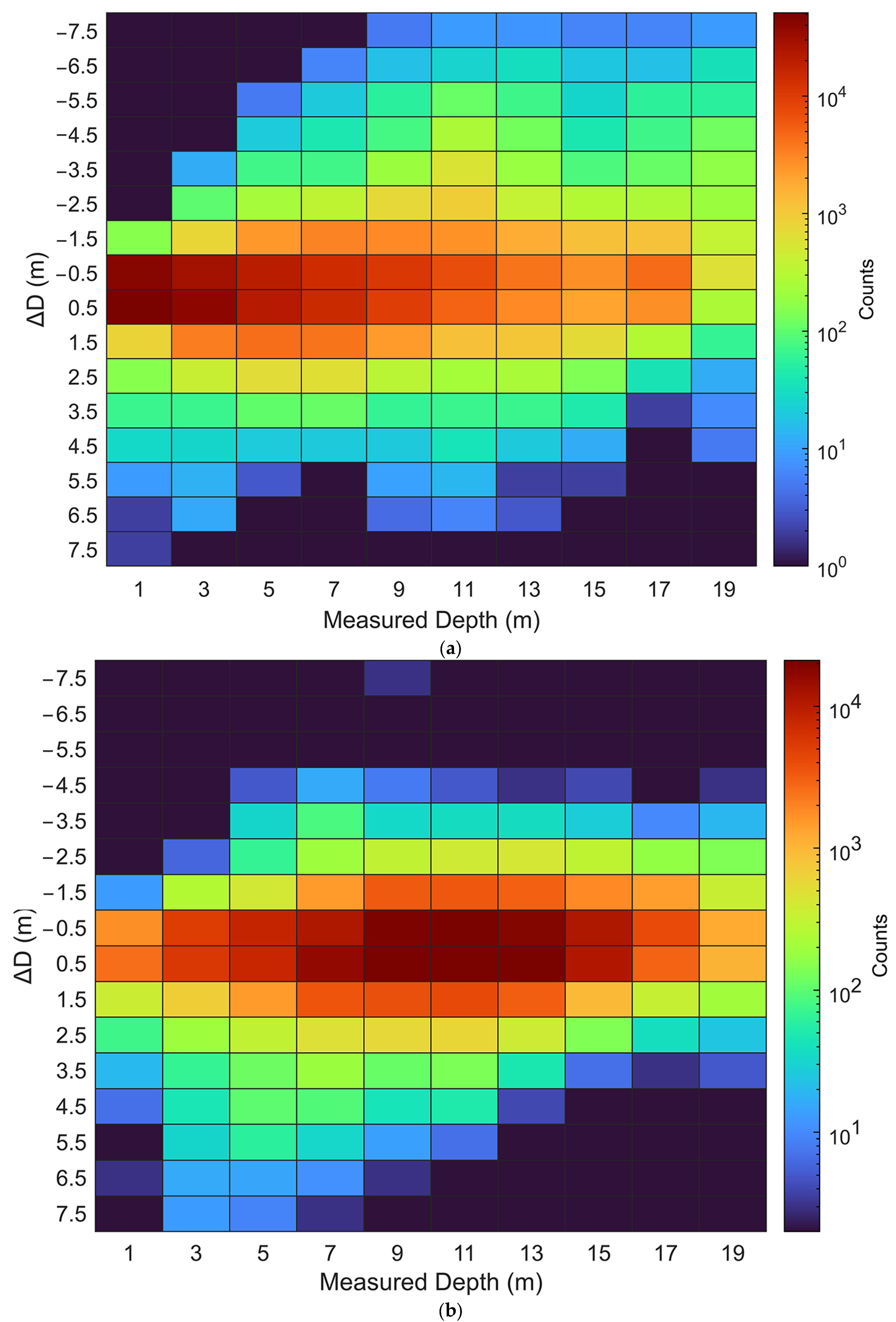
Figure 16 shows heatmaps of inversion error versus the measured water depth. Figure 16a shows that for Oahu Island, approximately 89.2% of the pixels with |∆D| ≤ 1 m, and 94.7% with |∆D| ≤ 1.5 m. Shallow-water areas (at depths of 0–8 m) have predominantly positive errors, indicating that the depth inversion in shallow areas is prone to overestimation. At depths of 8–20 m, negative errors are more common, with the majority of errors underestimated by more than 5 m occurring at depths of 8–20 m. Figure 14b clearly shows the spatial distribution of inversion errors (|∆D| ≥ 1.5 m), mainly at the lagoon-fringing reef boundary, tidal channels, and image edges, where larger errors occur in areas of rapid depth change. Figure 14b shows that the spatial distribution trends of both are similar to Figure 5d.
Similarly, Figure 16b shows that for Buck Island, approximately 88.4% of the pixels have an inversion error of |∆D| ≤ 1 m, while 95.1% of the errors are within Δ D 1.5   m . These proportions are very close to those for Oahu Island, suggesting that the histogram distribution of water depth (Figure 3b and Figure 4b) has a minimal effect on the inversion results of the four-band MDNhood model. Figure 16b shows negative errors primarily in the lagoon area and deep-water regions of the northern and northeastern sections of the image, while positive errors mainly occur in the entire northern deep-water area and the southern sections of the islands, where depth changes are significant. Comparing these results with those in Figure 6d, the spatial distribution trends are also similar.

4.3. Influence of the SSPBDD Phenomenon on the Depth Inversion via the MDNhood Model

The patterns of inversion depth error for Oahu Island and Buck Island are similar to those of the maximum depth difference of the SSPBDD pixels in Figure 5d and Figure 6d, respectively. It is necessary to analyse the correlation between the inversion error and the SSPBDD phenomenon to determine whether the main source of the inversion depth error is from the larger maximum depth difference of the SSPBDD pixels. The following analysis focuses on three-band (B2, B3, and B4) SSPBDD due to the high proportion, which is more representative, as shown in Table 2, rather than four-band SSPBDD.
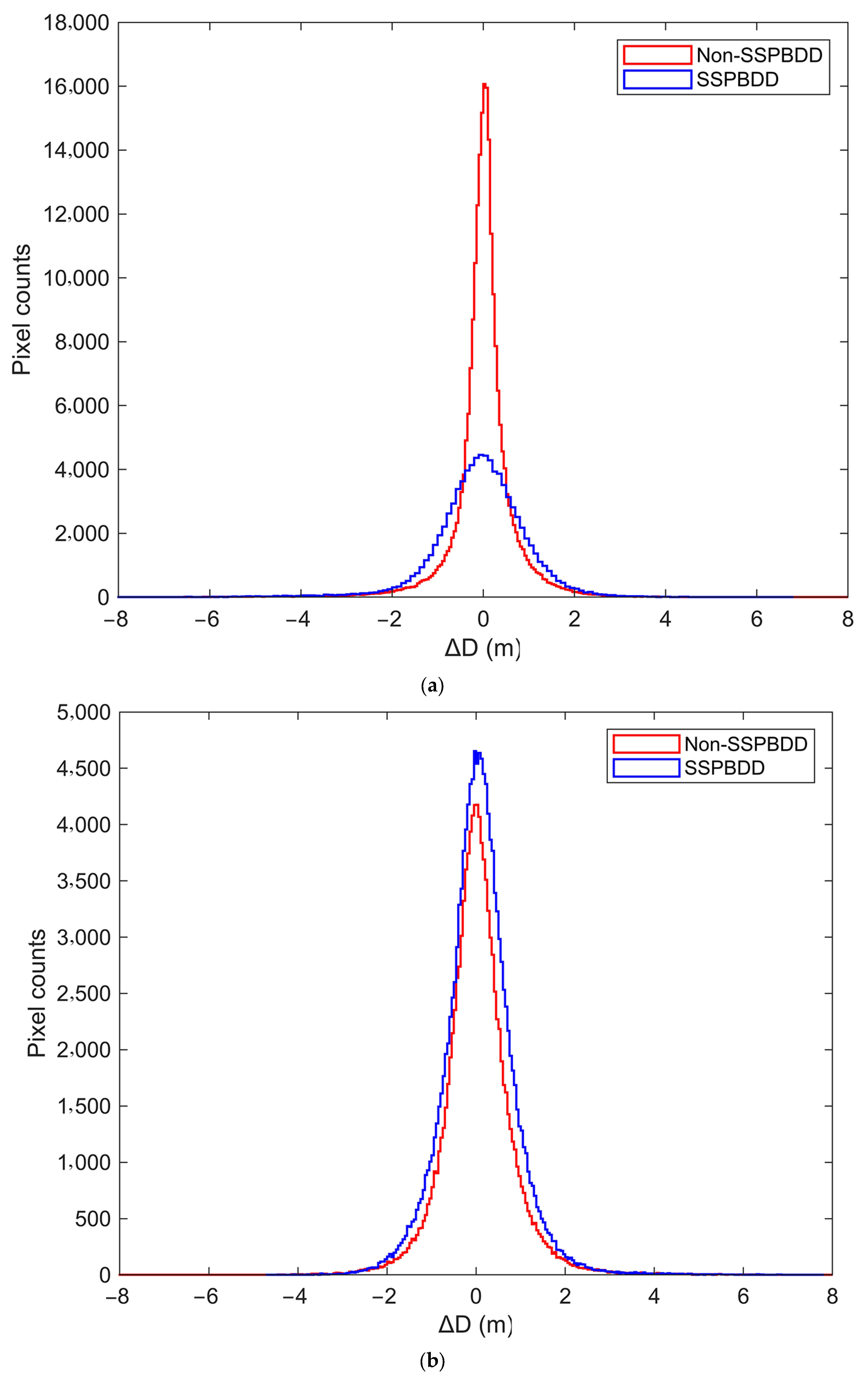
Figure 17 shows histograms for the SSPBDD and non-SSPBDD pixels for Oahu Island and Buck Island, respectively. Although the percentage of the SSPBDD pixels for Oahu Island is only 26.3%, as shown in Table 2, the number of pixels with inversion errors of |∆D| ≥ 1 m is greater than the number of non-SSPBDD pixels in Figure 17a, which indicates that the contribution of the SSPBDD pixels to the inversion errors is significant when |∆D| ≥ 1 m for Oahu Island. For Buck Island, the percentage of SSPBDD pixels (56.0%) is slightly greater than that of non-SSPBDD pixels in Table 2, so SSPBDD pixels account for a majority of the inversion errors. The shapes of the histogram curves in Figure 17 are similar to those of the Gaussian distribution f x = e x p x μ 2 / 2 σ 2 / 2 π σ , with the SSPBDD curve for Oahu Island exhibiting a larger σ parameter. The difference between the σ parameters of the SSPBDD curve and non-SSPBDD curve is quite small for Buck Island, suggesting that the presence of the SSPBDD phenomenon reduces the inversion error accuracy of the four-band MDNhood model. However, based on the RMSE of the four models in Figure 10, Figure 11, Figure 12 and Figure 13, it is evident that the MDNhood model can generally reduce the impact of the SSPBDD phenomenon (Figure 10 and Figure 11), but it cannot fully eliminate it.
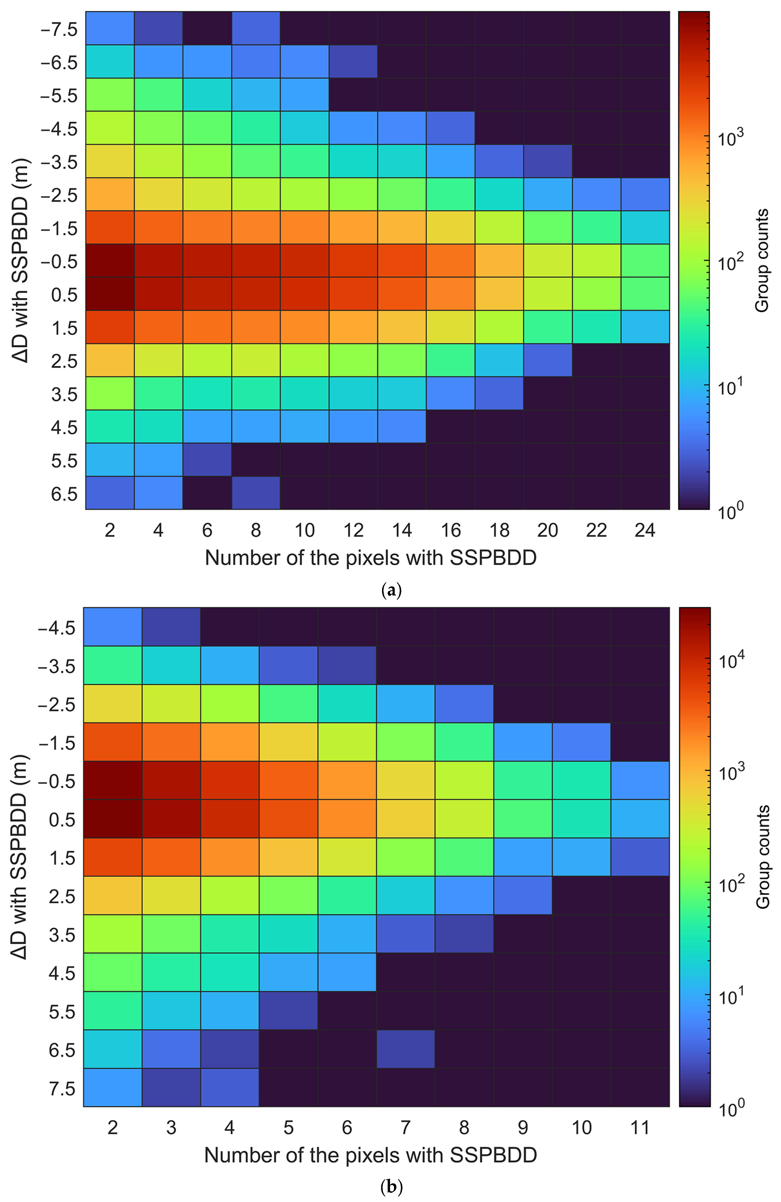
To analyse the relationship between the inversion error ΔD and the number of pixels in a group with the SSPBDD, Figure 18 shows heatmaps of the number for Oahu Island and Buck Island, respectively, relative to ΔD. Most of the group counts have a smaller number of pixels and smaller ΔD, and the inversion error ΔD decreases as the number increases, indicating that the probability of a large error is higher with a lower number of SSPBDD pixels.
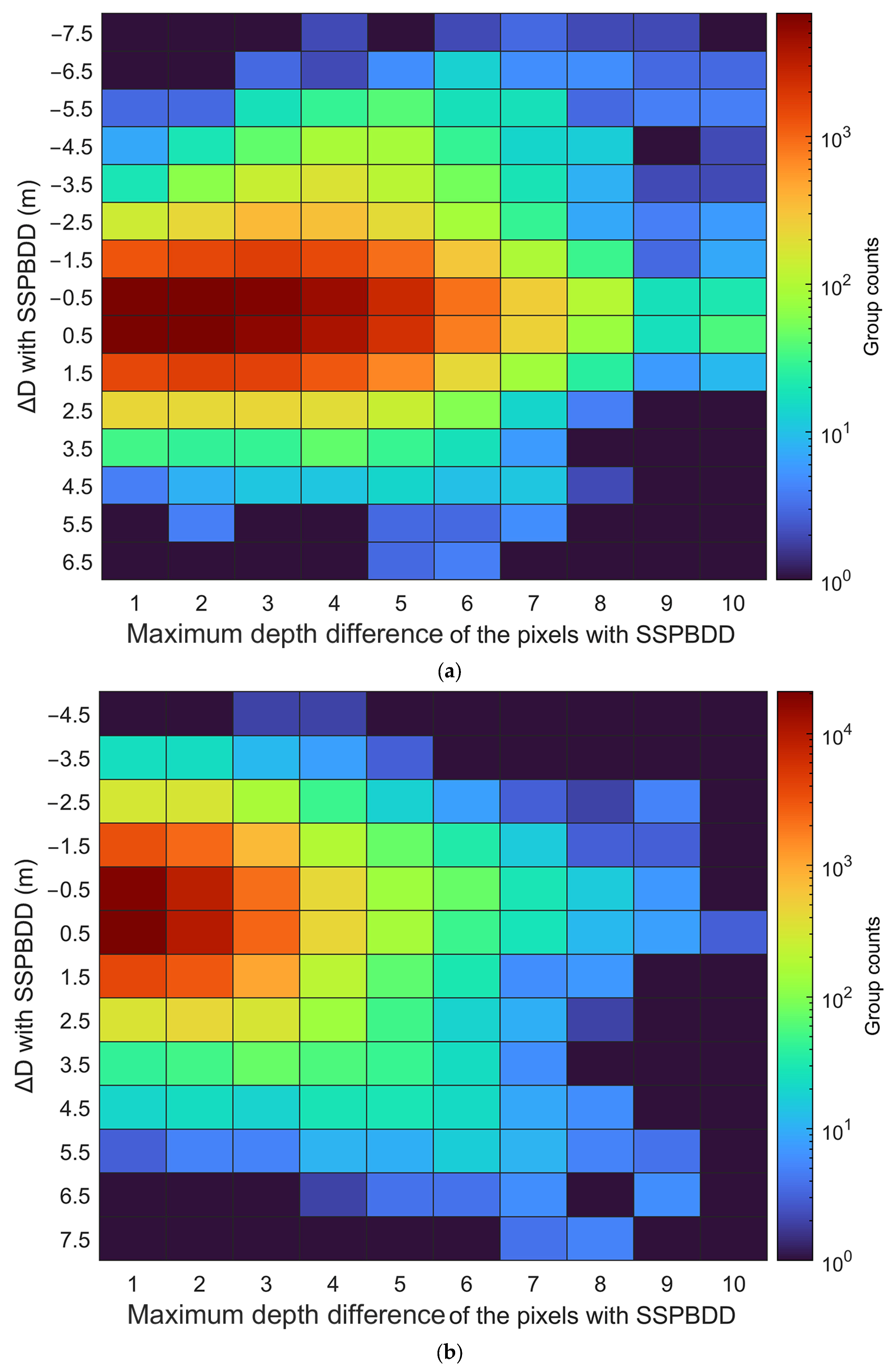
Figure 19 shows the heatmaps of the maximum depth difference with the SSPBDD pixels in a group vs. the inversion error for Oahu Island and Buck Island, respectively. Similar to Figure 18, most of the group counts are in the narrower maximum depth difference of pixels and the smaller ΔD, but the relationship between the maximum depth difference values and ΔD is not significantly correlated, the probability of a larger ΔD is greater for a wider maximum depth difference.
The above analysis can further explain why the inversion errors for Oahu Island are larger than those for Buck Island, even though the percentage of three-band SSPBDD pixels for Oahu Island is lower than that for Buck Island in Table 2. In fact, the number of SSPBDD pixels in a group reaches 25 for Oahu Island, and the group counts are more than those for Buck Island. Furthermore, the group counts in the wider maximum depth difference of the SSPBDD pixels are more than those for Buck Island.

5. Discussion

In fact, Sentinel-2 OLI sensor is not sufficient to capture fine-scale signals from the water column, which is not designed for remote sensing of water colour [7,8]. In addition, there are other factors such as different substrate types, water constituents, depth, incomplete atmospheric correction, and neighbourhood mixture, etc. When only two, three, or four optical bands are used for the shallow water depth inversion, there are cases where the spectral profiles are identical but the corresponding water depths are different (the SSPBDD phenomenon); i.e., there is the one-to-many relationship between the spectral profile and the water depth. This relationship causes uncertainties in the shallow water depth inversion and reduces the inversion accuracy. To avoid this effect as much as possible, more bands or combinations of bands that can represent the information on substrate type, water constituents, depth, etc., should be added into the input-layer vector; e.g., for Sentinel-2, band B1 has a greater impact on reducing the SSPBDD phenomenon than band B4, because band B1 provides richer spectral information (Table 2) and improves the accuracy of the depth inversion. However, the spatial distribution of the water depth and its corresponding spectral profile is not negligible information and can represent, to some extent, the relationship between neighbouring image pixels [4,22]. Adding spatial neighbourhood information can increase the spatial heterogeneity and reduce the SSPBDD phenomenon, but selecting the best optimal structure and the hyperparameters for machine learning models are difficult. Therefore, although this paper refers to the MDN models from [32,33], it still cannot eliminate the effect of the SSPBDD phenomenon.
Although the experimental design of this paper uses only 10 sampling runs, which seems to represent the stability (the standard deviation of RMSE) of the four models, a more rigorous design should include additional random sampling to cover various underwater terrains and water body spectral profiles to demonstrate the impact of training datasets on the inversion accuracy of the four models. The Stumpf model shows surprisingly high stability, with a high correlation coefficient between the log-transformed dual-band logarithmic ratio and water depth. However, its accuracy is lower, possibly due to the use of only the B2 and B3 bands and the high percentage of the SSPBDD pixels for the two bands. The stability of the MDN model is second; this model is constructed based on a Gaussian mixture density model and more suitable for handling one-to-many data distributions (i.e., multimodal distributions). The input layer of the MDN model includes spectral bands, depth-invariant indices, and spatial neighbourhood parameters, this spectral dimension and spatial dimension information can effectively improve the accuracy and stability of the model. In contrast, for the RF and SVM models, the inversion accuracy and stability are relatively poor, perhaps due to insufficient training dataset size, sensitivity to spatial distribution, or unsuitable model structure and hyperparameters, which are common issues for machine learning models.
Although the overall inversion accuracy of the MDN model is relatively high, there are still a small percentage of cases with larger errors (absolute error greater than 1.5 m) in the results (Figure 14, Figure 15, Figure 16, Figure 17, Figure 18 and Figure 19). These larger errors (Figure 14 and Figure 15) are mainly found in areas with significant spatial variations in underwater terrain, such as tidal channels, lagoons, coral reefs, image boundaries and deeper areas. The spectral–depth uniqueness is high, and the models may not be sufficiently trained. To address the decrease in inversion model accuracy caused by the SSPBDD, it is necessary to increase the size of the training dataset and optimise the structure of the inversion model to make full use of all spectral dimension and spatial dimension information.
Figure 3 and Figure 7 demonstrate that the distribution of water depth is non-Gaussian, while the water depth inversion model is a mixture of probabilistic densities. Interestingly, the errors in water depth inversion adhere to a Gaussian distribution. The one-to-many relationship is the main reason, as is shown by the histograms of the depth of pixels with the SSPBDD in Figure 5 and Figure 6. However, the true cause requires further in-depth analysis with additional data.

6. Conclusions

This paper presents a statistical analysis of the SSPBDD phenomenon within the depth of 0–20 m using Sentinel-2 satellite multispectral images based on water depth inversion models such as Stumpf, Random Forest (RF), Support Vector Machine (SVM), and Mixture Density Network (MDN) for Oahu Island and Buck Island. Information such as the blue–green band ratio, (Depth Invariant Index) DII, and spatial neighbourhood information are incorporated into the machine learning models. The root mean square error (RMSE) is used as a metric to evaluate the accuracy of these models, and the effect of random training datasets with different spatial distributions on the depth inversion are investigated. The following conclusions are drawn:
(1)
The SSPBDD phenomenon is observed in a relatively high percentage of the pixels. However, the more bands used, the fewer pixels there are with the SSPBDD. The percentage of the SSPBDD pixels is lower in shallower water (0–5 m) and deeper water (≥15 m), while it is higher in intermediate depths (5 m–15 m), where the satellite spectral information is dominated by the water body information, and the bottom substrate information plays a secondary role. These results suggest that these areas are prone to the SSPBDD phenomenon.
(2)
The RF model and the SVM model show considerable changes in RMSE under the influence of different spatial distributions in the training datasets, while the Stumpf model and the MDN model are the least affected. However, the Stumpf model typically achieves the lowest inversion accuracy.
(3)
The SSPBDD phenomenon can reduce the accuracy of water depth inversion models, the number and the maximum depth difference of the SSPBDD pixels in a group are the main influencing factors. Adding optical bands not only effectively decreases the percentage of SSPBDD pixels but also improves the inversion accuracy of the machine learning models. After incorporating the dual-band logarithmic ratio, DII, and spatial neighbourhood information, the MDN models show a more significant improvement in water depth inversion accuracy. Compared to the other models, the MDN model better handles the uncertainty caused by the SSPBDD phenomenon and the spatial distribution of the training dataset.
Based on these conclusions, this study provides a comprehensive and highly accurate water depth inversion model that utilizes multispectral and neighbourhood information while effectively reducing the errors caused by the SSPBDD phenomenon. However, this study only uses satellite imagery from two images of specific regions, and further application of the MDN model to additional regions and satellite imagery is needed to evaluate its robustness. Estimating the uncertainty associated with bathymetry predictions is crucial to understand the reliability of the results. Researchers are developing methods to quantify and visualize the uncertainty in bathymetry estimations [34,35], which can help inform decision-making and guide further data collection efforts. This will be the further direction of this study to improve the accuracy, efficiency, and applicability of bathymetry estimation in various coastal environments.

Author Contributions

Conceptualization, B.C.; methodology, E.H. and B.C.; formal analysis, B.C.; satellite data processing: B.C. and K.L.; writing—original draft preparation, E.H., B.C. and S.C. All authors have read and agreed to the published version of the manuscript.

Funding

This work was funded by the National Natural Science Foundation of China (Grant #42176178); the Scientific Research Foundation of Third Institute of Oceanography, MNR (2020011); the Open Fund of Beijing Engineering Research Centre for Aerospace Intelligent Remote Sensing Equipment (AIRSE202302); the National High Resolution Special Research (Grant 41-Y30F07-9001-20/22); the Scientific Research Foundation of Third Institute of Oceanography, MNR (2020017).

Data Availability Statement

The Sentinel-2 Level 2 dataset (https://scihub.copernicus.eu/ accessed on: 14 May 2024), the bathymetry dataset (https://www.coast.noaa.gov/dataviewer/ accessed on: 14 May 2024), and the tide data (https://tidesandcurrents.noaa.gov accessed on: 14 May 2024) are publicly archived datasets. The processed data used to construct the figures presented in this paper are available upon reasonable request from the corresponding author ([email protected]).

Conflicts of Interest

The authors declare no conflicts of interest.

References

  1. Ma, Y.; Xu, N.; Liu, Z.; Yang, B.; Yang, F.; Wang, X.H.; Li, S. Satellite-Derived Bathymetry Using the ICESat-2 Lidar and Sentinel-2 Imagery Datasets. Remote Sens. Environ. 2020, 250, 112047. [Google Scholar] [CrossRef]
  2. Duplančić Leder, T.; Baučić, M.; Leder, N.; Gilić, F. Optical Satellite-Derived Bathymetry: An Overview and WoS and Scopus Bibliometric Analysis. Remote Sens. 2023, 15, 1294. [Google Scholar] [CrossRef]
  3. Zhongqiang, W.; Mao, Z.; Wei, S.; Yuan, D.; Zhang, X.; Haiqing, H. Satellite-Derived Bathymetry Based on Machine Learning Models and an Updated Quasi-Analytical Algorithm Approach. Opt. Express 2022, 30, 16773–16793. [Google Scholar]
  4. Li, N.; Tang, Q.; Chen, Y.; Dong, Z.; Li, J.; Fu, X. Satellite-Derived Bathymetry Integrating Spatial and Spectral Information of Multispectral Images. Appl. Opt. 2023, 62, 2017–2029. [Google Scholar] [CrossRef]
  5. Lumban-Gaol, Y.; Ohori, K.A.; Peters, R. Extracting Coastal Water Depths from Multi-Temporal Sentinel-2 Images Using Convolutional Neural Networks. Mar. Geod. 2022, 45, 615–644. [Google Scholar] [CrossRef]
  6. Casal, G.; Harris, P.; Monteys, X.; Hedley, J.; Cahalane, C.; McCarthy, T. Understanding Satellite-Derived Bathymetry Using Sentinel 2 Imagery and Spatial Prediction Models. GISci. Remote Sens. 2020, 57, 271–286. [Google Scholar] [CrossRef]
  7. Dörnhöfer, K.; Göritz, A.; Gege, P.; Pflug, B.; Oppelt, N. Water Constituents and Water Depth Retrieval from Sentinel-2A—A First Evaluation in an Oligotrophic Lake. Remote Sens. 2016, 8, 941. [Google Scholar] [CrossRef]
  8. Pizani, F.; Maillard, P.; Ferreira, A.F.F.; de Amorim, C.C. Estimation of water quality in a reservoir from Sentinel-2 MSI and Landsat-8 OLI sensors. ISPRS Ann. Photogramm. Remote Sens. Spat. Inf. Sci. 2020, 3, 401–408. [Google Scholar] [CrossRef]
  9. Zhang, A.D. Principle and Application of Remote Sensing; Science Press: Alexandria, Australia, 2016. [Google Scholar]
  10. Walter, V. Object-Based Classification of Remote Sensing Data for Change Detection. ISPRS J. Photogramm. Remote Sens. 2004, 58, 225–238. [Google Scholar] [CrossRef]
  11. Chang, C.; Zhao, G.; Wang, L.; Zhu, X.; Gao, Z. Land Use Classification Based on RS Object-Oriented Method in Coastal Spectral Confusion Region. Nongye Gongcheng Xuebao/Trans. Chin. Soc. Agric. Eng. 2012, 28, 226–231. [Google Scholar]
  12. Howari, F.; Goodell, P. Characterization of Salt-Crust Build-Up and Soil Salinization in the United Arab Emirates by Means of Field and Remote Sensing Techniques. In Remote Sensing of Soil Salinization; CRC Press: Boca Raton, FL, USA, 2008; pp. 141–152. [Google Scholar]
  13. Seafloor Substrate (Hard and Soft Bottom) Maps at Select Islands and Atolls in American Samoa, the Mariana Archipelago, and the Pacific Remote Island Areas|InPort. Available online: https://www.fisheries.noaa.gov/inport/item/34310 (accessed on 15 July 2023).
  14. Cordeiro, M.C.R.; Martinez, J.-M.; Peña-Luque, S. Automatic Water Detection from Multidimensional Hierarchical Clustering for Sentinel-2 Images and a Comparison with Level 2A Processors. Remote Sens. Environ. 2021, 253, 112209. [Google Scholar] [CrossRef]
  15. International Hydrographic Organization. IHO Standards for Hydrographic Surveys (S-44), 5th ed.; International Hydrographic Organization: Commune de Monaco, Monaco, 2008. [Google Scholar]
  16. Yang, H.; Ju, J.; Guo, H.; Qiao, B.; Nie, B.; Zhu, L. Bathymetric Inversion and Mapping of Two Shallow Lakes Using Sentinel-2 Imagery and Bathymetry Data in the Central Tibetan Plateau. IEEE J. Sel. Top. Appl. Earth Obs. Remote Sens. 2022, 15, 4279–4296. [Google Scholar] [CrossRef]
  17. Casal, G.; Hedley, J.D.; Monteys, X.; Harris, P.; Cahalane, C.; McCarthy, T. Satellite-Derived Bathymetry in Optically Complex Waters Using a Model Inversion Approach and Sentinel-2 Data. Estuar. Coast. Shelf Sci. 2020, 241, 106814. [Google Scholar] [CrossRef]
  18. Albright, A.; Glennie, C. Nearshore Bathymetry from Fusion of Sentinel-2 and ICESat-2 Observations. IEEE Geosci. Remote Sens. Lett. 2021, 18, 900–904. [Google Scholar] [CrossRef]
  19. Lyzenga, D.R. Shallow-water reflectance modelling with applications to remote sensing of ocean floor. Int. Symp. Remote Sens. Environ. 1979, 13, 583–602. [Google Scholar]
  20. Chen, B.Q.; Yang, Y.M.; Xu, D.W.; Huang, E.H. A dual band algorithm for shallow bathymetric inversion from high spatial resolution imagery with no ground truth. ISPRS J. Photogramm. Remote Sens. 2019, 151, 1–13. [Google Scholar] [CrossRef]
  21. Afrasinei, G.; Melis, M.; Arras, C.; Pistis, M.; Buttau, C.; Ghiglieri, G. Spatiotemporal and Spectral Analysis of Sand Encroachment Dynamics in Southern Tunisia. Eur. J. Remote Sens. 2018, 51, 352–374. [Google Scholar] [CrossRef]
  22. Wang, Y.; Zhou, X.; Li, C.; Chen, Y.; Yang, L. Bathymetry Model Based on Spectral and Spatial Multifeatures of Remote Sensing Image. IEEE Geosci. Remote Sens. Lett. 2020, 17, 37–41. [Google Scholar] [CrossRef]
  23. Ai, B.; Wen, Z.; Wang, Z.; Wang, R.; Su, D.; Li, C.; Yang, F. Convolutional Neural Network to Retrieve Water Depth in Marine Shallow Water Area From Remote Sensing Images. IEEE J. Sel. Top. Appl. Earth Obs. Remote Sens. 2020, 13, 2888–2898. [Google Scholar] [CrossRef]
  24. Stumpf, R.P.; Holderied, K.; Sinclair, M. Determination of water depth with high-resolution satellite imagery over variable bottom types. Limnol. Oceanogr. 2003, 48 Pt 2, 547–556. [Google Scholar] [CrossRef]
  25. Lyzenga, D.R.; Malinas, N.P.; Tanis, F.J. Multispectral bathymetry using a simple physically based algorithm. IEEE Trans. Geosci. Remote Sens. 2006, 44, 2251–2259. [Google Scholar] [CrossRef]
  26. Zhou, W.; Tang, Y.; Jing, W.; Li, Y.; Yang, J.; Deng, Y.; Zhang, Y. A Comparison of Machine Learning and Empirical Approaches for Deriving Bathymetry from Multispectral Imagery. Remote Sens. 2023, 15, 393. [Google Scholar] [CrossRef]
  27. Breiman, L. Random Forests. Mach. Learn. 2001, 45, 5–32. [Google Scholar] [CrossRef]
  28. Drucker, H.; Burges, C.; Kaufman, L.; Smola, A.; Vapnik, V. Support Vector Regression Machines. Adv. Neural Inform. Process. Syst. 1997, 28, 779–784. [Google Scholar]
  29. Bishop, C.M. Mixture Density Networks. 1994. Available online: https://research.aston.ac.uk/en/publications/mixture-density-networks (accessed on 15 June 2023).
  30. Saranathan, A.M.; Pahlevan, N. Multi-Parameter Retrieval of Water Quality Indicators from Bayesian and Mixture Density Networks. In Proceedings of the IGARSS 2023—2023 IEEE International Geoscience and Remote Sensing Symposium, Pasadena, CA, USA, 16–21 July 2023; pp. 3946–3949. [Google Scholar]
  31. Kun-tang, C.; Xiaolong, D.; Xingou, X.; Shuyan, L. The Study on Oceanic Vector Wind Field Retrieve Technique Based on Neural Networks of Microwave Scatterometer. Remote Sens. Technol. Appl. 2017, 32, 683–690. [Google Scholar]
  32. Smith, B.; Pahlevan, N.; Schalles, J.; Ruberg, S.; Errera, R.; Ma, R.; Giardino, C.; Bresciani, M.; Barbosa, C.; Moore, T.; et al. A Chlorophyll-a Algorithm for Landsat-8 Based on Mixture Density Networks. Front. Remote Sens. 2021, 1, 623678. [Google Scholar] [CrossRef]
  33. Pahlevan, N.; Smith, B.; Schalles, J.; Binding, C.; Cao, Z.; Ma, R.; Alikas, K.; Kangro, K.; Gurlin, D.; Hà, N.; et al. Seamless Retrievals of Chlorophyll-a from Sentinel-2 (MSI) and Sentinel-3 (OLCI) in Inland and Coastal Waters: A Machine-Learning Approach. Remote Sens. Environ. 2020, 240, 111604. [Google Scholar] [CrossRef]
  34. Saranathan, A.; Smith, B.; Pahlevan, N. Pahlevan Per-Pixel Uncertainty Quantification and Reporting for Satellite-Derived Chlorophyll-a Estimates via Mixture Density Networks. IEEE Trans. Geosci. Remote Sens. 2023, 61, 1–18. [Google Scholar] [CrossRef]
  35. Zolfaghari, K.; Pahlevan, N.; Simis, S.G.H.; O’Shea, R.E.; Duguay, C.R. Sensitivity of Remotely Sensed Pigment Concentration via Mixture Density Networks (MDNs) to Uncertainties from Atmospheric Correction. J. Great Lakes Res. 2023, 49, 341–356. [Google Scholar] [CrossRef]
  36. Mixture Density Network for Water Constituent Estimation. Available online: https://github.com/BrandonSmithJ/MDN (accessed on 15 June 2023).
  37. Philpot, W. Bathymetric Mapping with Passive Multispectral Imagery. Appl. Opt. 1989, 28, 1569–1578. [Google Scholar] [CrossRef]
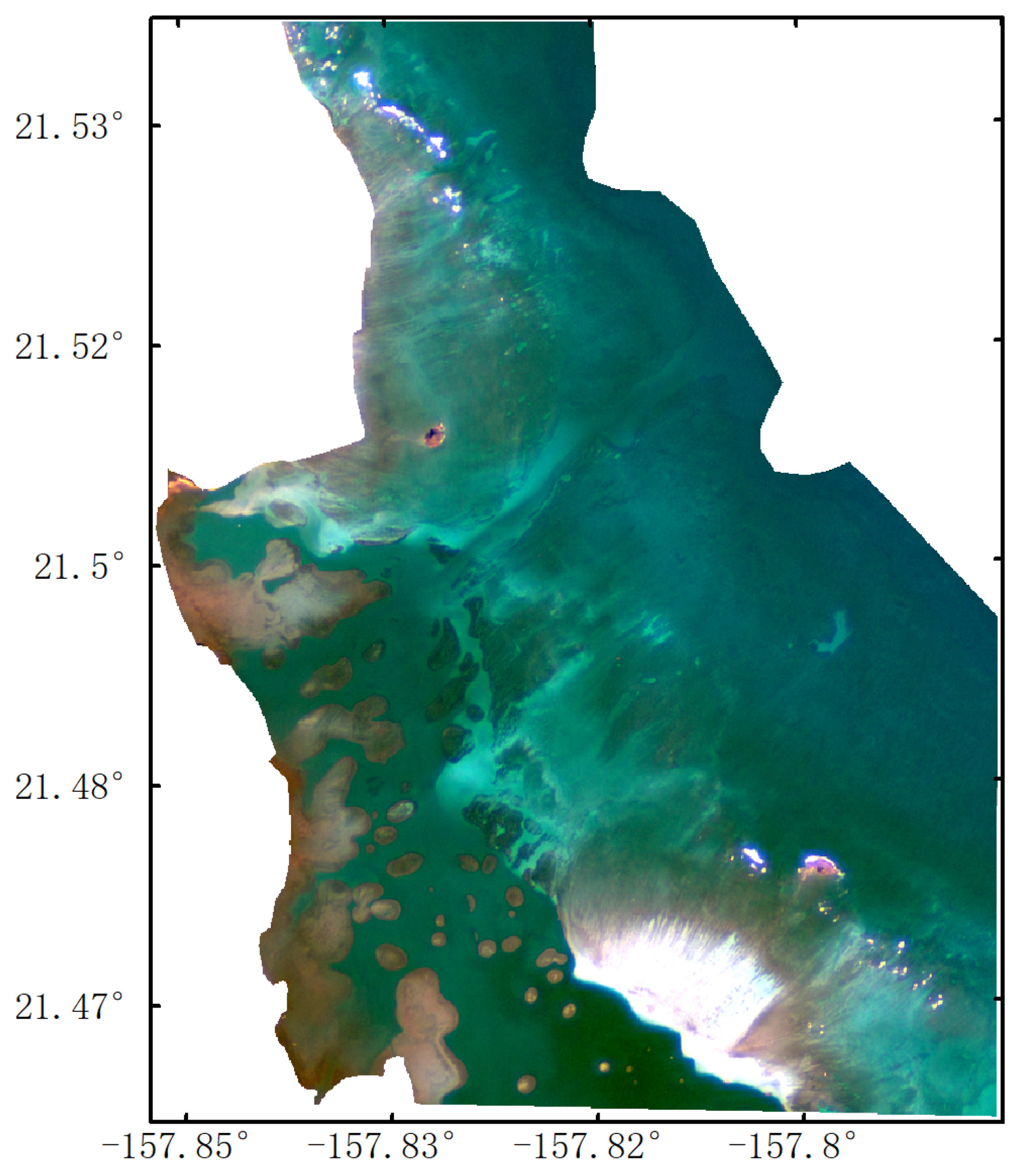
Figure 1. Sentinel-2B images of Oahu Island.
Remotesensing 16 01759 g001
Figure 2. Sentinel-2A images of Buck Island.
Remotesensing 16 01759 g002
Figure 3. Measured depths (a) and depth histogram (b) of Oahu Island.
Remotesensing 16 01759 g003aRemotesensing 16 01759 g003b
Figure 4. Measured depths (a) and depth histogram (b) of Buck Island.
Remotesensing 16 01759 g004aRemotesensing 16 01759 g004b
Figure 5. Histogram (ac) and the spatial distribution (d) of pixels with the SSPBDD on Oahu Island. (a) histogram of number of the pixels with the SSPBDD in a group, Pixels with the same spectral profile form a group. (b) histogram of depth of pixels with the SSPBDD. (c) histogram of maximum depth difference of the pixels with the SSPBDD in a group. (d) the spatial distribution of the pixels with the SSPBDD, only pixels with a maximum depth difference greater than or equal to 1.5 m.
Remotesensing 16 01759 g005aRemotesensing 16 01759 g005bRemotesensing 16 01759 g005c
Figure 6. Histogram and the spatial distribution of pixels with the SSPBDD on Buck Island. (a) histogram of number of the pixels with the SSPBDD in a group, Pixels with the same spectral profile form a group. (b) histogram of depth of pixels with the SSPBDD. (c) histogram of maximum depth difference of the pixels with the SSPBDD in a group. (d) the spatial distribution of the pixels with the SSPBDD, only pixels with a maximum depth difference greater than or equal to 1.5 m.
Remotesensing 16 01759 g006aRemotesensing 16 01759 g006b
Figure 7. Structural schematic diagram of the Mixture Density Network. The subscript number of the character ‘h’ represents the serial number of the hidden layer, which ranges from 1 to 5, and vi, μ i , σ i , and α i , respectively, represent the i-th node, weight coefficient, mean, and variance, where the subscript i ranges from 1 to 100.
Remotesensing 16 01759 g007
Figure 8. Error bars of models with different band combinations for Oahu Island. The blue marker represents two-band only for Stumpf model; the red markers represent three-band (Equation (5), or Equation (7)); the yellow markers represent four-band (Equation (6), or Equation (8)). To avoid overlap, three-band marker and four-band markers are located on each side of gridlines corresponding to the label of the model’s name. There are some markers, e.g., the blue marker of the Stumpf model, the three-band and the four-band marker of the MDN model, for which the error bars are unclear, i.e., standard deviation of RMSE is very small. Error bars of three-band model of SVM and SVMhood is exceptionally large, which denotes the standard deviation of their RMSEs are very big. The representations in Figure 9, Figure 10, Figure 11, Figure 12 and Figure 13 are similar.
Remotesensing 16 01759 g008
Figure 9. Error bars of models with different band combinations for Buck Island.
Remotesensing 16 01759 g009
Figure 10. Error bars of models with different band combinations for only SSPBDD pixels for Oahu Island.
Remotesensing 16 01759 g010
Figure 11. Error bars of models with different band combinations for only SSPBDD pixels for Buck Island.
Remotesensing 16 01759 g011
Figure 12. Error bars of models with different band combinations for only non-SSPBDD pixels for Oahu Island.
Remotesensing 16 01759 g012
Figure 13. Error bars of models with different band combinations for only non-SSPBDD pixels for Buck Island.
Remotesensing 16 01759 g013
Figure 14. Inversion depth imagery (a) and only the pixels with Δ D > 1.5 m (b) for Oahu Island. Only 0–20 m water depth is shown, other depths are left blank for (a). To show more clearly where the pixels with larger errors are located, only Δ D > 1.5 m is plotted, and others are blank in (b). The representation in Figure 13 is similar.
Remotesensing 16 01759 g014aRemotesensing 16 01759 g014b
Figure 15. Inversion depth imagery (a) and only the pixels with Δ D > 1.5   m   (b) for Buck Island.
Remotesensing 16 01759 g015
Figure 16. Heatmaps of depth-predicted errors for Oahu Island (a) and Buck Island (b).
Remotesensing 16 01759 g016
Figure 17. Histogram of ΔD with the SSPBDD pixels and ΔD with the non-SSPBDD pixels for Oahu Island (a) and Buck Island (b).
Remotesensing 16 01759 g017
Figure 18. Heatmap of the number of pixels with the SSPBDD in a group for Oahu Island (a) and Buck Island (b), respectively. It denotes the relationship between ΔD and number of the pixels with SSPBDD in a group, most of which are inversely proportional.
Remotesensing 16 01759 g018
Figure 19. Histogram of the maximum depth difference with the SSPBDD in a group for Oahu Island (a) and Buck Island (b), respectively. They show that there is no significant correlation between ΔD and maximum depth difference in contrast to Figure 18.
Remotesensing 16 01759 g019
Table 1. Characteristics of the Sentinel-2 images used in this paper.
SatelliteRegionAcquisition Time (UTC)Tide Height
(m)
Product LevelBand and Spectral Range
(nm)
Spatial Resolution
(m)
Sentinel-2BOahu Island2020-12-01 21:090.29Level 2AB1: 433–45360
B2: 458–523
B3: 543–578
B4: 650–680
10
Sentinel-2ABuck Island2022-01-29 14:570.71
Table 2. Percentage of pixels with the SSPBDD for different band combination on Buck Island and Oahu Island.
Band CombinationPercentage of Pixels with the SSPBDD/All Water Pixels within 020 m on Oahu IslandPercentage of Pixels with the SSPBDD/All Water Pixels within 0–20 m on Buck Island
B2, B3124,662/328,514 ≈ 37.9%233,398/251,867 ≈ 92.7%
B2, B3, B486,513/328,514 ≈ 26.3%141,093/251,867 ≈ 56.0%
B1, B2, B3, B412,188/328,514 ≈ 3.7%1878/251,867 ≈ 0.7%
Disclaimer/Publisher’s Note: The statements, opinions and data contained in all publications are solely those of the individual author(s) and contributor(s) and not of MDPI and/or the editor(s). MDPI and/or the editor(s) disclaim responsibility for any injury to people or property resulting from any ideas, methods, instructions or products referred to in the content.