Envelope Extraction Algorithm for Magnetic Resonance Sounding Signals Based on Adaptive Gaussian Filters

Abstract

Magnetic resonance sounding is a geophysical method for quantitatively determining the state for groundwater storage that has gained international attention in recent years. However, the practical acquisition of magnetic resonance sounding signals, which are on the nanovolt scale, is susceptible to various types of interference, such as power-line harmonics, random noise, and spike noise. Such interference can degrade the quality of magnetic resonance sounding signals and, in severe cases, be completely drowned out by noise. This paper introduces an adaptive Gaussian filtering algorithm that is well-suited for handling intricate noise signals due to its adaptive solving characteristics and iterative sifting approach. Notably, the algorithm can process signals without relying on prior knowledge. The adaptive Gaussian filtering algorithm is applied for the envelope extraction of noisy magnetic resonance sounding signals, and the reliability and effectiveness of the method are rigorously validated. The simulation results reveal that, even under strong noise interference (with original signal-to-noise ratios ranging from −7 dB to −25 dB), the magnetic resonance sounding signal obtained after algorithmic processing is compared to the ideal signal, with 16 sets of data statistics, and the algorithm ensures an initial amplitude uncertainty within 4nV and restricts the uncertainty of the relaxation time within a 6 ms range. The signal-to-noise ratio can be boosted by up to 53 dB. The comparative assessments with classical algorithms such as empirical mode decomposition and the harmonic modeling method confirm the superior performance of the adaptive Gaussian filtering algorithm. The processing of the field data also fully proved the practical application effects of the algorithm.

1. Introduction

Magnetic resonance sounding (MRS), also known as surface nuclear magnetic resonance (SNMR), is a geophysical exploration method that utilizes the natural geomagnetic field for groundwater imaging [1]. In comparison to the traditional geophysical exploration methods, such as the transient electromagnetic method, seismic surveys, and the multi-electrode resistivity method, the MRS method is currently an internationally advanced method for the direct quantitative detection of groundwater. Hydrogeological information such as groundwater content, burial depth, and aquifer thickness can be provided by inverse interpretation without drilling [2]. Consequently, since its introduction, this method has found widespread application in various domains, including water resource detection and assessment, dam leakage monitoring, tunnel seepage analysis, and mine water inflow prediction [3,4,5].

However, the MRS signal is a weak nanovolt-level signal, and, in practical applications, it is highly susceptible to the interference from power-line harmonics, random noise, and occasional spike noise, which leads to the signal being submerged in the ambient noise and makes it difficult to realize the effective extraction of the signal. The extraction of MRS signals has been a focal point of international research [6].

The extraction of MRS signals typically involves two main approaches. The first approach is the classical processing workflow. Addressing the three types of typical noise present in MRS signals, different strategies are employed for the noise removal. Subsequently, the MRS signal is extracted through data fitting.

To address spike noise, Jiang et al. [7] proposed the use of statistical stacking to eliminate the spike noise from the signal. In most cases, this method reduces the measurement time by nearly 50%, but it is not effective for small-amplitude peaks. Dalgaard et al. [8] introduced an energy calculation method that effectively detects and highlights small-amplitude spike noise, making it suitable for the detection and removal of the minor spikes occurring during the measurement process. Larsen [9] proposed to realize noise filtering by modeling the spike noise as a unit impulse response of two different second-order bandpass filters cascaded together. However, due to the overlap between the magnetic resonance sounding signal and spike noise, this approach may lead to overfitting. Lin et al. [10] suggested a denoising method combining empirical mode decomposition and wavelet thresholding, but it requires manually setting the thresholds.

Addressing power-line harmonic noise, Larsen et al. [11] proposed a modeling-based harmonic noise removal method in 2014. This method determines the model parameters of harmonic noise through least squares fitting and subtracts the modeled noise from the noisy signal. However, in the case of large relaxation times, it is difficult to extract better results. Recognizing the asynchronous variations in the harmonic noise in the main and reference coils, Li et al. [12] introduced a frame denoising method based on frequency-domain multi-channel Wiener filtering, which further enhances the denoising effectiveness. Nonetheless, this method may erroneously filter out magnetic resonance sounding signals when the Larmor frequency is close to the power-line frequency. Jiang et al. [13] proposed an elimination method based on the synchronous extraction transform that effectively removes the harmonic noise from a single record and simultaneously addresses multiple harmonic noises in stacking data. However, this method is not suitable for low-noise scenarios and cannot handle co-frequency harmonics. Researchers have also specifically investigated co-frequency harmonic removal. Liu et al. [14] used the relationship between the amplitude and phase of the co-frequency harmonics in the two coils established during noise-only segments to estimate the co-frequency harmonics in the primary coil based on the co-frequency model of the reference coil, and the co-frequency harmonics can be modeled using the data from the reference coil. Wang et al. [15] first used a standard harmonic modeling method to remove the harmonic components other than the co-frequency harmonics, followed by the nonlinear fitting of the noisy MRS signal containing the co-frequency harmonics. They proposed an efficient fundamental frequency search method based on magnitude square coherence (MSC), significantly reducing the computation time while ensuring computational accuracy.

For the removal of random noise, Legchenko et al. [16] suggested a stacking method. However, its effectiveness is severely limited in low-signal-to-noise-ratio environments, and multiple data acquisitions decrease the instrument efficiency. Ge et al. [17] proposed to combine improved wavelet thresholding with exponentially weighted moving averaging to reduce the noise in nuclear magnetic resonance (NMR) transversal data, and applied a particle swarm optimization algorithm to ensure stability and global convergence. Lin et al. [18] proposed the time–frequency peak filtering method to suppress random noise. They segmented the full-wave magnetic resonance sounding signal, encoded it into the instantaneous frequency of the analytic signal, and achieved unbiased signal estimation by extracting the peak values from the time–frequency distribution. However, the suppression effect is less satisfactory when the signal-to-noise ratio is low. In 2021, Lin et al. [19] introduced an improved short-time Fourier transform method to suppress random noise, using the analytic signal instead of the real-valued signal in conventional short-time Fourier transform to obtain the high-precision time–frequency distribution of the MRS signal. They then extracted the peak amplitude and phase values in the time–frequency domain to reconstruct the signal, effectively extracting the signal when the signal-to-noise ratio is higher than −17.21 dB.

Another approach in the MRS signal extraction process is to directly extract the envelope of the MRS signal, effectively achieving noise removal during the signal extraction process.

Currently, the commonly used international methods for extracting the envelopes of MRS signals include empirical mode decomposition (EMD) [20] and complete ensemble empirical mode decomposition (CEEMD), directly realizing the extraction of the MRS signal envelope [21]. However, both methods suffer from mode mixing issues and only achieved satisfactory results at high signal-to-noise ratios. Liu et al. [22] proposed a spectral analysis (SA) method based on sliding windows for recovering the envelopes of MRS signals in noisy environments, but this method is not suitable for extracting the envelopes of MRS signals with multiple components. Tian et al. [23] introduced an extraction algorithm using adaptive local iterative filtering using the Fokker–Planck equation solution as the filtering function. This method makes the filter function change adaptively during the decomposition process and is suitable for MRS signals with multiple components.

Additionally, noise removal methods based on deep learning networks for MRS signals have been proposed. These methods adaptively learn the features of input signals through the network, enabling the effective extraction of the measured MRS signal envelope. Lin et al. [24] presented a denoising framework based on Dn-ResUnet, achieving adaptive denoising and effectively recovering the signals in high-noise environments. Jiang et al. [25] proposed a noise suppression method based on a time–frequency fully convolutional neural network capable of simultaneously removing various types of noise with high computational efficiency.

In this study, we first introduced the basic principles of an adaptive Gaussian filter. Utilizing the adaptive Gaussian filter as the filter coefficient, we could extract several intrinsic mode function (IMF) components and their residuals. Combining the residuals generated iteratively from the real part with those from the imaginary part, we obtained the desired envelope. Subsequently, two key parameters of the Gaussian filter, the masking coefficient and the decomposition order, are determined, using the uncertainties of the initial amplitude and the relaxation time and the degree of signal-to-noise ratio improvement as the evaluation criteria. The performance simulation experiments were conducted under different signal-to-noise ratios, relaxation times, and Larmor frequencies. Finally, the proposed method was applied to field data, demonstrating its ability to extract the envelopes of MRS signals under complex noise interference without prior knowledge and providing accurate data information for the inverse interpretation of hydrological signals.

2. Principles and Methods

2.1. Magnetic Resonance Soundings Principles

MRS is based on the resonance transition of hydrogen protons in groundwater to realize the detection of groundwater [26]. The instrument system injects transmitting currents into coils laid on the ground. To satisfy the resonance condition, the transmitting pulse is set equal to the local geomagnetic field’s Larmor frequency. This alternating current creates an alternating magnetic field, and the hydrogen protons in the groundwater are excited by this alternating magnetic field, which creates a macroscopic magnetic moment that excites the hydrogen protons in the groundwater to produce a Larmor precession. The excitation field is usually withdrawn after 40 ms of excitation. Hydrogen protons return to their initial equilibrium state, releasing energy outward and generating a magnetic resonance sounding signal response with an exponential decay, which is captured by the instrument system. This constitutes the fundamental principle of magnetic resonance sounding for groundwater detection, as illustrated in Figure 1.

The mathematical model for the MRS signals collected by the instrument system can be expressed as follows:

$$S\left(t\right)=E_0{e}^{-\frac{t}{T_2^{*}}}cos(2\pi f_L+\phi )+noise\left(t\right)$$

(1)

Formula (1) represents the MRS signal, where $E_0$ denotes the initial amplitude, reflecting the magnitude of groundwater content. $T_2^{*}$ denotes the average transverse relaxation time, typically ranging between 30 ms and 1000 ms, indicating the porosity of the groundwater-bearing medium. $f_L$ represents the Larmor frequency, directly proportional to the magnitude of the geomagnetic field in the experimental area. $\phi$ denotes the initial phase, representing the lithological parameters of the subsurface medium. noise(t) represents environmental noise, including the combined effects of various types of noise, such as occasional spike noise, power-line harmonic noise, and random white noise.

Figure 2 illustrates the time-domain and frequency-domain plots of the MRS signal, incorporating three types of noise. Clearly visible in the time domain is the spike noise, whereas, in the frequency domain, harmonic interference fixed at integer multiples of the power-line frequency is observable. Additionally, wide-ranging random noise is present.

2.2. Principles of Adaptive Gaussian Filters

Gaussian filter is a type of linear smoothing filter that selects weights based on the shape of the Gaussian function. Gaussian smoothing filters are highly effective in suppressing noise that follows a normal distribution.

Given this, Yue-Der Lin et al. [27] devised an adaptive Gaussian filter based on the Gaussian window function $w\left(k\right)$ derived from (2). Through derivation and calculation, they obtained the mathematical expression of the discrete-domain Gaussian smoothing filter $w_G\left(k\right)$ as (3).

$$w\left(k\right)=e^{-\frac{k^2}{2{\sigma }^2}}=e^{-\frac{1}{2}{\left(\frac{k}{M/\alpha }\right)}^2}$$

(2)

$$w_G\left(k\right)=\frac{w\left(k\right)}{{\sum }_{l=-M}^{M}w\left(l\right)}$$

(3)

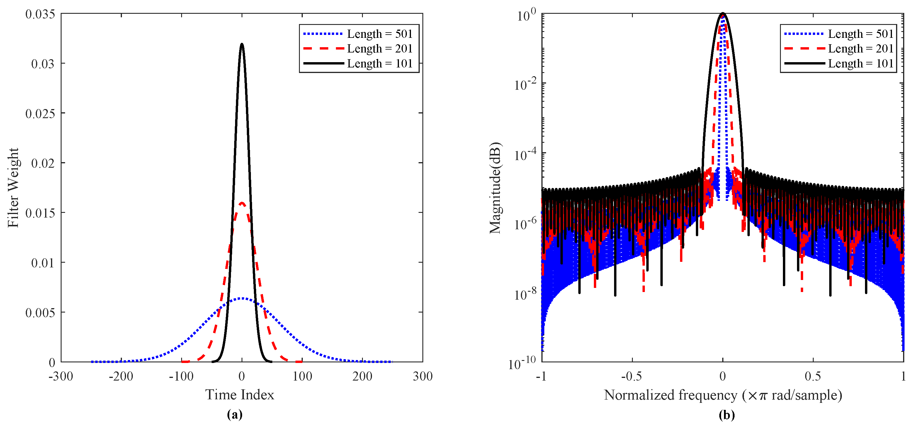
In this context, $\sigma =M/\alpha$, where $\alpha$ is a parameter inversely proportional to the standard deviation $\sigma$ and k is an integer within the range [$-M$,M]. The parameter L represents the length of the Gaussian filter, provided by $L=2M+1$. Figure 3 illustrates the time-domain and frequency-domain plots of the adaptive Gaussian filter for different filter lengths.

Suppose the signal to be processed is denoted as $s\left(n\right)$, ($0\le n\le N-1$). The steps for applying adaptive Gaussian filtering to the signal are as follows:

• Firstly, determine the parameter M for the adaptive Gaussian filter. This parameter is closely related to the length L of the Gaussian filter, where $L=2M+1$, and $⌊·⌋$ denotes the floor function.

  $$M=2·⌊\lambda \frac{N}{N_e}⌋$$

  (4)
  In (4), the parameter $\lambda$ ranges between 1.0 and 3.0, N represents the length of the signal $s\left(n\right)$, and $N_e$ denotes the number of extremal points in the signal.
• The signal $s\left(n\right)$ is extended at its endpoints using a combination of the “constant”, “periodic”, “mirroring”, and “bidirectional symmetric mirroring” methods. The choice of extension method depends on the characteristics of the signal to be processed, obtaining the extended signal $s_e\left(n\right)$.
• For the extended signal $s_e\left(n\right)$, smoothing filtering is applied using the Gaussian filter from (3). This process obtains the instantaneous mean signal:

  $$m_i\left(n\right)={\sum }_{k=-M}^M{w}_G\left(k\right)s_e(k+n)$$

  (5)
• Determination of IMF components based on (6), and the stopping criterion for sifting satisfies (7), where the value of $\eta$ is greater than 20 [27]. If this condition is met, the decomposition stops; otherwise, the process is repeated from steps 1 to 4.

  $$r_i\left(n\right)=s\left(n\right)-m_i\left(n\right)$$

  (6)

  $$\eta =10{log}_{10}\frac{{∥s(·)∥}^2}{{∥r_i(·)∥}^2}$$

  (7)
  In this context, $r_i\left(n\right)$ represents the ith IMF component.

Following the aforementioned adaptive Gaussian filtering process, the signal to be decomposed can be expressed as

$$s\left(n\right)={\sum }_{i=1}^m{r}_i\left(n\right)+org\left(n\right)$$

(8)

In (8), $org\left(n\right)$ represents the residual information after signal decomposition.

3. Results

To validate the performance of the adaptive Gaussian filter algorithm, a series of algorithmic simulation experiments were conducted using MATLAB 2022a. The reference of the selected computer is an Intel(R) Core(TM) i7-10700 CPU.

3.1. Implementation of the Gaussian Filter Algorithm

Initially, we simulated the generation of MRS signals with an initial amplitude $E_0$ of 100 nV, a relaxation time $T_2^{*}$ of 200 ms, a Larmor frequency of 2325 Hz, and an initial phase of $\frac{\pi }{3}$. Building upon this foundation, we constructed 16 sets of noisy MRS signals by introducing power-line harmonic noise and random noise. The fundamental frequency of the power-line harmonic noise was randomly generated within the range of $50\pm 0.01$ Hz, with an amplitude in the range of ($0,100$), phase in the range of ($-\pi ,\pi$) radians, and an order of 80. The random noise was modeled as Gaussian white noise with a standard deviation of 100 nV. The adaptive Gaussian filter was applied for processing, and Figure 4 illustrates the resulting IMF components obtained by processing the real and imaginary parts of the MRS signal. The real and imaginary components are synthesized, and the synthesis result of the residual is used as the extracted MRS signal envelope. Figure 5 presents the time-domain and frequency-domain plots of the MRS signal before and after the algorithmic processing.

3.2. Selection of Algorithm Parameters

In the process of algorithm implementation, two key parameters affecting the algorithm’s performance are the mask coefficient and the decomposition order. The range for the mask coefficient typically falls between 1.0 and 3.0. The decomposition order is usually chosen to be greater than 2, and, in our case, we selected values between 2 and 20. This range was chosen because a higher decomposition order inevitably leads to more complex computational requirements, impacting the algorithm efficiency. The performance of the algorithm is typically characterized by the uncertainty of the initial amplitude, relaxation time, and the improvement in the signal-to-noise ratio.

$${\sigma }_{E_0}=\sqrt{\frac{{\sum }_{i=1}^N{(E_{0i}-\overline{E_0})}^2}{N(N-1)}}$$

(9)

$${\sigma }_{T_2^{*}}=\sqrt{\frac{{\sum }_{i=1}^N{(T_{2i}^{*}-\overline{T_2^{*}})}^2}{N(N-1)}}$$

(10)

$$snr=10 lg\frac{{∥s\left[·\right]∥}^2}{{∥n\left[·\right]∥}^2}$$

(11)

We systematically varied the mask coefficient from 1.0, with intervals of 0.2, up to 3.0, and iterated through decomposition orders ranging from 2 to 20. The contour plots of the initial amplitude and relaxation time and the degree of signal-to-noise improvement corresponding to different mask coefficients and decomposition orders were obtained, as shown in Figure 6. The MRS signals and noise parameters generated in the experiments are the same as in Section 3.1.

From Figure 6a,b, it is evident that the deep blue regions correspond to areas where the uncertainty of the fitted results for the initial amplitude and relaxation time is minimized, as can be seen by the fact that the corresponding filter decomposition order can be found for different masking coefficients. In Figure 6c, the yellow region signifies areas with relatively high enhancements in signal-to-noise ratio. The positions marked with “★” denote the locations with the highest signal-to-noise ratio enhancement.

Therefore, weighing the uncertainty in the initial amplitude and the relaxation time, as well as the value of the signal-to-noise enhancement, all the program parameters in this thesis were chosen to be a combination of a masking coefficient of 1.6 and a decomposition order of 8.

3.3. Comparison with Other Algorithms

To further illustrate the performance of the algorithm, a comparative analysis was conducted between the adaptive Gaussian filter algorithm, the empirical mode decomposition (EMD) algorithm, and the harmonic modeling algorithm. Both the adaptive Gaussian filter and EMD algorithms utilize iterative sifting methods to obtain individual component signals. In the GSF algorithm, the sliding operator is constructed by filtering the decomposed signal. The EMD method uses cubic spline interpolation to obtain the envelope.

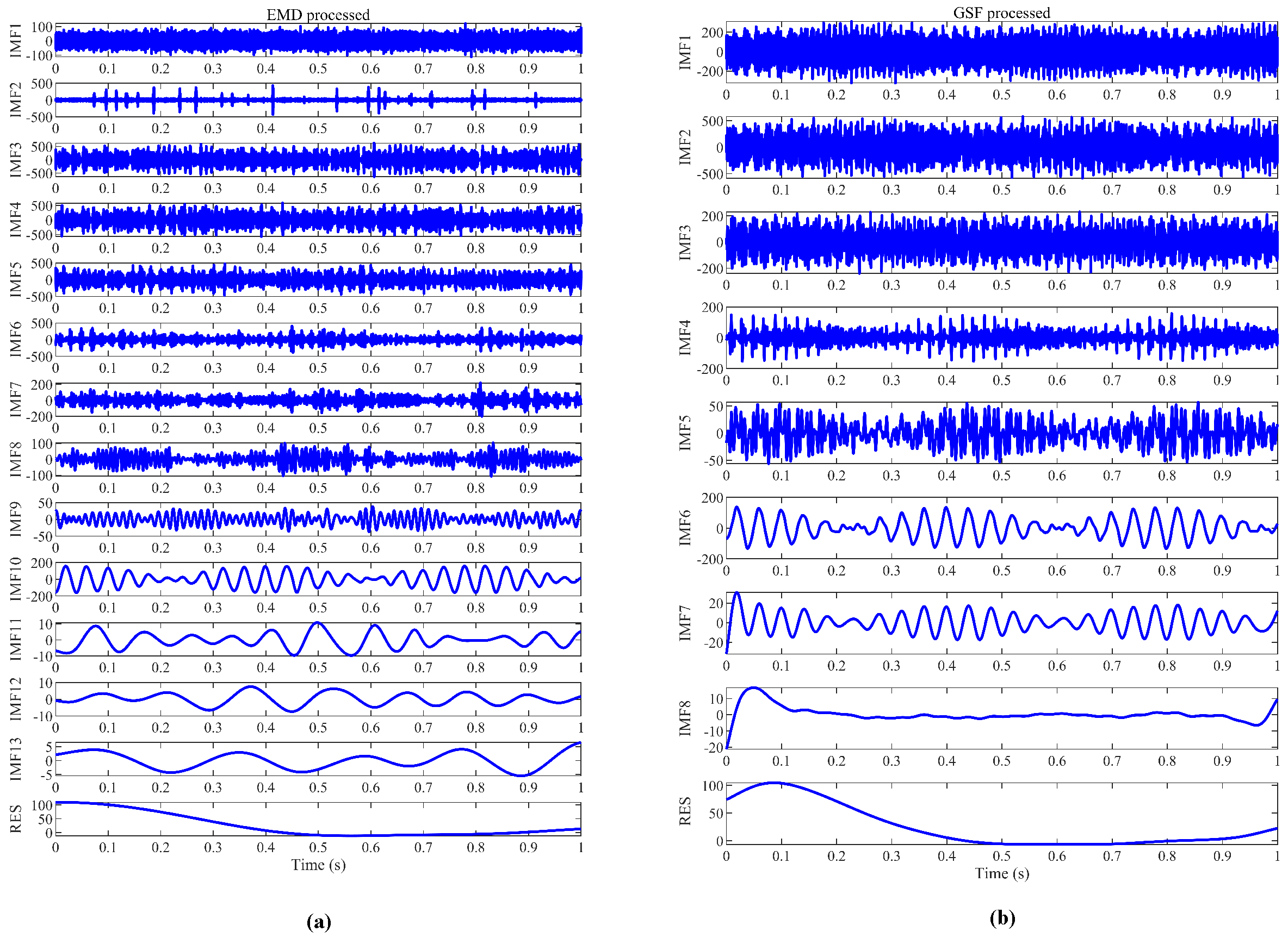
To construct a noisy signal model, we simulated the generation of MRS signals with an initial amplitude $E_0$ of 200 nV, a relaxation time $T_2^{*}$ of 200 ms, a Larmor frequency of 2325 Hz, and an initial phase of $\frac{\pi }{3}$. We then added power-line harmonic noise and random noise. The fundamental frequency of the power-line harmonic noise was randomly generated within the range of 50 ± 0.01 Hz, with the amplitude in the range of (0, 100) nV, the phase in the range of ($-\pi ,\pi$) radians, and an order of 80. The random noise was modeled as Gaussian white noise with a standard deviation of 100 nV. The noisy signals were processed using the EMD algorithm, GSF algorithm, and harmonic modeling algorithm. Figure 7 illustrates each IMF component and residual obtained using EMD and GSF, whereas Figure 8 displays the outcomes of the three algorithms for the noisy MRS signal model. It is evident that the results obtained by the EMD algorithm show a smaller initial amplitude and certain fluctuations in the MRS signal envelope, indicating limitations related to endpoint effects and mode mixing issues. The harmonic modeling algorithm effectively eliminates the influence of power-line harmonics but struggles to suppress the random noise due to limited superposition iterations. In summary, the GSF algorithm demonstrates superior extraction performance, highlighting its advantages in this context.

3.4. Processing of Field Data

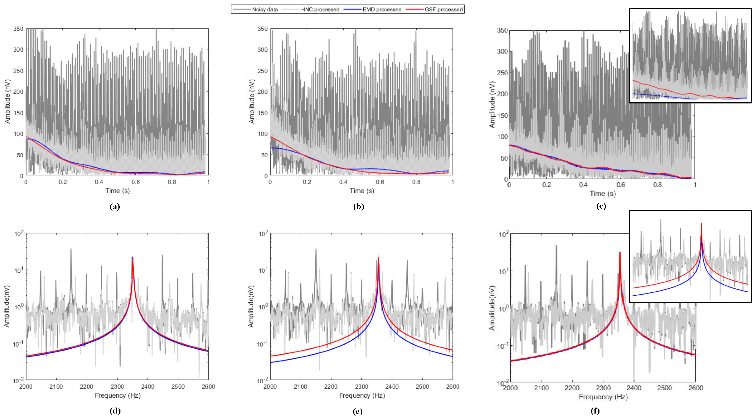
To validate the practicality of the adaptive Gaussian filter algorithm, field measurements were conducted using the JLMRS-III magnetic resonance sounding instrument at the Cultural Square. During the data acquisition, the MRS signals were generated using a signal source with a sampling rate of 25,000 Hz. The collected noisy MRS signals were obtained by combining the receiving coil with ambient complex noise. Three sets of noisy MRS signals with different geological conditions were selected for processing, the signal envelope was obtained after adaptive Gaussian filtering, and the processing results are depicted in Figure 9.

Table 1. Comparative analysis of algorithms for field signals.

Group	Larmor Frequency (Hz)	Method	${\mathit{snr}}_{\mathit{old}}$ (dB)	${\mathit{snr}}_{\mathit{pro}}$ (dB)	$\mathbf{\Delta }\mathit{snr}$ (dB)	${\mathit{E}}_0$ (nV)	${\mathit{E}}_{0_{\mathit{fit}}}$ (nV)	${\mathit{T}}_2^{*}$ (ms)	${\mathit{T}}_{2_{\mathit{fit}}}^{*}$ (ms)
		HNC	−9.27	0.86	10.13		101.12		203.79
1	2351	EMD	−9.27	17.11	26.38	102	102.09	200	212.91
		GSF	−9.27	24.93	34.20		100.97		197.19
		HNC	−8.20	2.73	10.93		80.80		204.43
2	2355	EMD	−8.20	16.99	25.19	80	76.28	200	198.97
		GSF	−8.20	23.93	32.13		76.99		201.72
		HNC	−8.11	2.93	11.04		84.68		417.73
3	2355	EMD	−8.11	22.82	30.93	86	86.07	400	397.13
		GSF	−8.11	24.30	32.41		84.35		406.95

provides a performance comparison between the proposed GSF method, the existing EMD algorithm, and the harmonic modeling algorithm.

4. Discussion

In practical applications, the stability of adaptive Gaussian filtering is a paramount concern that demands focused attention. The stability of the algorithm directly impacts its reliability across various noise environments. Considering factors such as the noise intensity, type, statistical characteristics, and potential variations in local Larmor frequencies, the algorithm must exhibit a certain level of robustness. Therefore, further research into the algorithm’s processing capabilities for different application scenarios and assessing the adaptability of adaptive Gaussian filtering in complex noise and diverse geological environments becomes indispensable. In this section, we will delve into the algorithm’s performance under varying conditions and its efficacy in both simulated and field signal contexts.

4.1. Performance Analysis of the Algorithm under Different Conditions

To validate the universality of the algorithm, we conducted performance analyses under varying signal-to-noise ratios, relaxation times, Larmor frequencies, and white noise amplitudes.

4.1.1. Investigation of Denoising Effectiveness under Different Signal-to-Noise Ratios

The parameters for generating MRS signals were set as described in Section 3.1. By altering the power-line harmonics amplitude, we obtained envelope extraction results under various initial signal-to-noise ratio conditions, as summarized in

Table 2. Analysis of noise cancellation effects of adaptive Gaussian filtering with different signal-to-noise ratios.

Group	${\mathit{snr}}_{\mathit{old}}$ (dB)	${\mathit{snr}}_{\mathit{pro}}$ (dB)	$\mathbf{\Delta }\mathit{snr}$ (dB)	${\mathit{E}}_{0_{\mathit{fit}}}$ (nV)	${\mathit{T}}_{2_{\mathit{fit}}}^{*}$ (ms)
1	−23.54	29.52	53.06	99.46 ± 3.30	201.54 ± 5.98
2	−21.94	29.25	51.19	99.98 ± 2.74	200.82 ± 5.53
3	−20.75	28.29	49.04	99.47 ± 2.47	201.66 ± 4.60
4	−16.72	34.15	50.87	99.47 ± 1.83	200.99 ± 3.69
5	−14.15	34.32	48.47	99.27 ± 1.07	201.73 ± 2.07
6	−7.47	37.93	45.40	99.31 ± 0.25	201.38 ± 0.59

. From Table 2, it is evident that, following the processing with the adaptive Gaussian filter algorithm, the enhancement in the signal-to-noise ratio ($\Delta$SNR) can exceed 53 dB. As the noise intensity increases and the signal-to-noise ratio decreases, the $\Delta$SNR value becomes larger, stabilizing at around 30 dB after processing. This indicates that the algorithm has stronger processing capabilities for signals with lower signal-to-noise ratios caused by an increase in the amplitude of the power-line harmonics. The fitting results for the initial amplitude and relaxation time indicate that the uncertainty in the initial amplitude remains within 4 nV, while the uncertainty in the relaxation time remains within a range of 6 ms. Such uncertainties in the initial amplitude and relaxation time can meet the accuracy requirements of the subsequent inversion results.

4.1.2. Investigation of Denoising Effectiveness under Different Relaxation Times

The parameters for generating the MRS signals were set as follows: initial amplitude $E_0$ of 100 nV, Larmor frequency of 2325 Hz, and initial phase of $\frac{\pi }{3}$. The Gaussian white noise and harmonic noise amplitudes were both set to 50 nV. Due to the stochastic nature of the simulated data, the results were obtained through statistical analysis, as presented in

Table 3. Analysis of noise cancellation effects of adaptive Gaussian filtering with different relaxation times.

Group	${\mathit{T}}_2^{*}$ (ms)	${\mathit{snr}}_{\mathit{old}}$(dB)	${\mathit{snr}}_{\mathit{pro}}$ (dB)	$\mathbf{\Delta }\mathit{snr}$ (dB)	${\mathit{E}}_{0_{\mathit{fit}}}$ (nV)	${\mathit{T}}_{2_{\mathit{fit}}}^{*}$ (ms)
1	100	−21.97	31.29	52.66	101.61 ± 3.14	99.18 ± 2.82
2	200	−18.19	31.73	49.92	100.08 ± 1.57	201.59 ± 3.20
3	300	−15.99	36.66	52.65	99.78 ± 1.26	299.27 ± 4.43
4	400	−14.54	34.93	49.47	99.09 ± 0.75	402.43 ± 3.35
5	500	−13.55	38.27	51.82	100.00 ± 0.82	496.81 ± 5.27
6	600	−12.70	32.93	45.63	99.07 ± 0.78	602.81 ± 5.43

. The data in Table 3 were derived from the statistical analysis of 16 sets of data under different relaxation time conditions. From Table 3, it can be observed that, with an increase in the relaxation time, the initial signal-to-noise ratio tends to decrease. After the processing with the adaptive Gaussian filter algorithm, the $\Delta$SNR can exceed 45 dB. As the relaxation time increases, the uncertainty in the initial amplitude gradually decreases, while the uncertainty in the relaxation time gradually increases. The uncertainty in the initial amplitude remains within 4 nV, and the uncertainty in the relaxation time remains within a range of 6 ms. Figure 10 presents the box plots of the fitting results under different relaxation times. ‘+’ denotes an outlier, which represents data that falls more than 1.5 times the interquartile distance above the third quartile or below the first quartile. It can be seen that, with an increase in the relaxation time, the interquartile range of the initial amplitude $E_0$ gradually decreases, while the interquartile range of $T_2^{*}$ gradually increases, consistent with the trends observed in the statistical results in Table 3.

Combining Table 3 and Figure 10, it can be seen that the algorithm yields relatively larger uncertainties in extracting the parameters for aquifers with longer relaxation times. This is consistent with the practical scenarios as the relaxation time represents the porosity of the subsurface media. Those exceeding 600 ms indicate flowing water bodies, while those within 300–600 ms correspond to the same type of media, namely gravel deposits. Therefore, even with slightly larger uncertainties, it does not lead to misjudgments of the lithology.

4.1.3. Investigation of Denoising Effectiveness under Different Larmor Frequencies

The parameters for generating MRS signals were set with an initial amplitude $E_0$ of 100 nV, a relaxation time $T_2^{*}$ of 200 ms, and an initial phase of $\frac{\pi }{3}$. The Gaussian white noise and harmonic noise amplitudes were both set to 50 nV. The results of the envelope extraction were statistically compiled for 16 instances under different Larmor frequency conditions, as presented in

Table 4. Analysis of noise cancellation effects of adaptive Gaussian filtering at different Larmor frequencies.

Group	${\mathit{f}}_{\mathit{L}}$ (Hz)	${\mathit{snr}}_{\mathit{old}}$ (dB)	${\mathit{snr}}_{\mathit{pro}}$ (dB)	$\mathbf{\Delta }\mathit{snr}$ (dB)	${\mathit{E}}_{0_{\mathit{fit}}}$ (nV)	${\mathit{T}}_{2_{\mathit{fit}}}^{*}$ (ms)
1	2300	−17.96	14.93	32.89	108.58 ± 5.52	200.12 ± 14.19
2	2310	−18.11	24.63	42.74	99.81 ± 1.90	200.59 ± 3.31
3	2320	−18.05	30.05	48.10	99.34 ± 1.68	201.74 ± 3.18
4	2330	−18.10	32.39	50.49	99.42 ± 1.39	200.95 ± 3.25
5	2340	−18.09	26.83	44.92	98.35 ± 1.96	200.49 ± 3.35
6	2350	−17.97	15.57	33.54	91.14 ± 7.59	224.65 ± 53.32
7	2360	−18.04	23.73	41.77	100.30 ± 1.75	198.08 ± 3.52
8	2370	−18.25	27.54	45.79	101.03 ± 1.80	199.62 ± 3.49

. From Table 4, it is evident that, under conditions with the presence of co-frequency harmonics, such as when $f_L$ is 2300 Hz and 2350 Hz, the fitting errors for $E_0$ and $T_2^{*}$ after the Gaussian filtering denoising are relatively large, and the measurement uncertainties are notably significant. Particularly, when $f_L$ is 2350 Hz, the uncertainty in the relaxation time exceeds 53 ms and is entirely unreliable. In other cases, the uncertainty in the initial amplitude is controlled within 2 nV, and the uncertainty in the relaxation time is limited to a range of 4 ms. Figure 11 presents the box plots of parameter fitting under different Larmor frequencies, aligning with the trends observed in Table 4.

Combining Table 4 and Figure 11 reveals that, for complete co-frequency harmonics interference, the algorithm in this paper lacks the processing capability. In such cases, specialized algorithms for co-frequency harmonics need to be employed.

4.1.4. Impact of Varying Noise Amplitudes on the Adaptive Gaussian Filter Algorithm

This section primarily investigates the effects of the white noise amplitude change on the signal parameter extraction and the impact of harmonic noise amplitude variation similar to white noise. Sixteen sets of repeated experiments were conducted, and the results were summarized in

Table 5. Adaptive Gaussian filtering noise cancellation effect analysis under different white noise amplitudes.

Group	White Noise Amplitude (nV)	${\mathit{snr}}_{\mathit{old}}$ (dB)	${\mathit{snr}}_{\mathit{pro}}$ (dB)	$\mathbf{\Delta }\mathit{snr}$ (dB)	${\mathit{E}}_{0_{\mathit{fit}}}$ (nV)	${\mathit{T}}_{2_{\mathit{fit}}}^{*}$ (ms)
1	100	−18.83	28.30	47.13	99.51 ± 1.70	201.30 ± 3.71
2	200	−21.20	23.06	44.26	99.58 ± 2.07	197.04 ± 5.40
3	300	−23.61	20.19	43.80	100.05 ± 2.11	198.88 ± 5.77
4	400	−25.59	15.47	41.06	101.37 ± 3.99	199.61 ± 5.89
5	500	−27.35	15.74	43.09	106.72 ± 4.27	199.43 ± 13.87
6	600	−28.73	12.27	41.00	108.11 ± 6.36	211.57 ± 16.87

. From Table 5, it is observed that, as the noise amplitude increases, the signal-to-noise ratio of the noisy MRS signal continuously decreases. When the signal-to-noise ratio of the processed signal falls within the range of −18 to −28, the $\Delta$SNR after filtering is at least 41 dB, reaching up to 47 dB. However, with the increase in the white noise amplitude, the uncertainties in the initial amplitude and relaxation time also increase. For white noise amplitudes below 400 nV, the uncertainty in the initial amplitude remains within 4 nV, and the uncertainty in the relaxation time is controlled within a range of 6 ms. When the white noise amplitude reaches 500 nV and above, the uncertainties in both the initial amplitude and relaxation time fitting increase.

White noise is the most challenging type of noise to handle in magnetic resonance sounding signals because of its wide frequency range, which overlaps with the signal spectrum, making it difficult to completely eliminate. Additionally, we only selected 16 sets of measurement data for statistical analysis, and the amplitude of the power-line harmonics is within a 100 nV range. Therefore, under these conditions, it is concluded that the noise amplitude with relatively good measurement uncertainty is below 400 nV. Increasing the number of experimental datasets can enhance the white noise processing capability.

4.2. Comparison of Simulation Data and Discussion of Field Data Processing Results

In order to evaluate the performance advantages and disadvantages of the adaptive Gaussian filtering algorithm proposed in this paper and the existing classical noise cancellation algorithms, algorithm comparison experiments were carried out based on simulation data. In order to make the simulation more in line with the actual situation, harmonic noise containing random fundamental frequency, random amplitude, and phases with white noise were added to construct the test signal. From the decomposition results of the GSF algorithm and the EMD algorithm in Figure 7, it can be seen that the EMD decomposition order is indeterminate, and it will adaptively decompose according to the characteristics of the signal, but, due to the endpoint effect as well as the existence of the modal aliasing problem, it leads to the initial amplitude of the extracted envelopes in Figure 8 being obviously small, and the signal fluctuation is obvious, which indicates that the noise removal is not clean enough. Regarding the GSF algorithm, on the other hand, although the initial amplitude of the first end is also slightly reduced compared to the theoretical value due to the effect of the filtering algorithm, the deviation is small, and the decay in the time domain is relatively smooth after the extraction, and the frequency domain is closer to the ideal signal, which demonstrates better performance. Similarly, in the comparison with the harmonic modeling algorithm, since the harmonic modeling method removes noise by fitting the harmonic components of the signal, it does not have any processing capability for random noise, and it can only suppress part of the impact of random noise through the superposition of the data; thus, in Figure 8, the HNC method still contains a large amount of random noise after processing as a result.

The results of the processing of three sets of data are shown in Figure 9 and Table 1. These three sets of data include two combinations of different Larmor frequencies and different relaxation times to represent the results of the data processing under three different geological conditions with different signal-to-noise ratios. For the set of data with the Larmor frequency of 2351 Hz, it can be shown that, when the magnetic resonance signal is not exactly the same frequency as the power-line harmonics and only differs by 1 Hz, the GSF algorithm in this paper can still obtain good processing results, which is also consistent with the conclusions of the simulation experiments. Moreover, the GSF algorithm is more advantageous than the HNC and EMD algorithms in terms of parameter extraction error and signal-to-noise ratio improvement. For the two sets of data with a Larmor frequency of 2355 Hz, the GSF algorithm performs better when the relaxation time is 200 ms; when the relaxation time is 400 ms, the results of the GFS algorithm and the EMD algorithm are roughly better than those of the HNC algorithm, but it is necessary to explain here that the processing results of the EMD algorithm at this time are the result of artificially combining the last IMF component and the residual as the to-be-extracted MRS signal envelope results; if only the residual is used as the MRS signal extraction envelope results, the EMD algorithm will present the situation of subgraphs, obviously detached from reality, which also confirms the defect that the EMD algorithm is prone to modal aliasing. As this field experiment is to use the signal source to simulate the groundwater signal, the signal-to-noise ratio of the signal is basically stable within −10 dB due to the fact that the noise intensity of the experimental collection environment is not as large as that of the simulation plus the uncertainty of the starting moment of the data collection by the instrument. The initial signal-to-noise ratio of the simulated data can reach below −20 dB, so the signal-to-noise ratio of the field data is only improved to more than 32 dB.

5. Conclusions

This study proposes an adaptive Gaussian filter algorithm based on the principles of Gaussian filtering and iterative sifting, addressing the Gaussian random noise and harmonic noise in noisy MRS signals. The algorithm aims to extract the envelopes from MRS, facilitating the extraction of reliable envelopes from low-signal-to-noise-ratio ground-based MRS to obtain high-quality data. The results confirm the effectiveness of the GSF algorithm in extracting the signal envelopes, with the uncertainty in the initial amplitude within 4 nV and the uncertainty in the relaxation time controlled within a range of 6 ms. The signal-to-noise ratio can be enhanced by up to 53 dB. The comparative analysis with classical algorithms such as the EMD algorithm and harmonic modeling algorithm demonstrates significant reductions in relative error, validating the superiority of the proposed algorithm. The accurate extraction of the MRS envelope signals holds profound significance for conducting detailed groundwater investigations under complex noise interference and predicting water-related hazards in mines/tunnels.

References

1. Hertrich, M. Imaging of groundwater with nuclear magnetic resonance. Prog. Nucl. Magn. Reson. Spectrosc. 2008, 53, 227–248. [Google Scholar] [CrossRef]
2. Legchenko, A.; Baltassat, J.M.; Beauce, A.; Bernard, J. Nuclear magnetic resonance as a geophysical tool for hydrogeologists. J. Appl. Geophys. 2002, 50, 21–46. [Google Scholar] [CrossRef]
3. Behroozmand, A.A.; Keating, K.; Auken, E. A review of the principles and applications of the NMR technique for near-surface characterization. Surv. Geophys. 2015, 36, 27–85. [Google Scholar] [CrossRef]
4. Jiang, C.; Liu, Z.; Li, B.; Lin, T.; Shang, X.; Diao, S.; Du, G.; Yi, X.; Lin, J. A Rotational Measurement Scheme of Surface Nuclear Magnetic Resonance for Shallow Frozen Lake Characterization in Urban Environments. IEEE Trans. Geosci. Remote Sens. 2022, 60, 5902512. [Google Scholar] [CrossRef]
5. Yang, Y.; Zhou, K.; Zhao, H.; Lin, T. Modeling of Surface Nuclear Magnetic Resonance Based on Prepolarization and Its Application in Urban Shallow Measurements. IEEE Trans. Geosci. Remote Sens. 2022, 60, 5916910. [Google Scholar] [CrossRef]
6. Lesparre, N.; Girard, J.F.; Jeannot, B.; Weill, S.; Dumont, M.; Boucher, M.; Viville, D.; Pierret, M.C.; Legchenko, A.; Delay, F. Magnetic resonance sounding measurements as posterior information to condition hydrological model parameters; application to a hard-rock headwater catchment. J. Hydrol. 2020, 587, 124941. [Google Scholar] [CrossRef]
7. Jiang, C.; Lin, J.; Duan, Q.; Sun, S.; Tian, B. Statistical stacking and adaptive notch filter to remove high-level electromagnetic noise from MRS measurements. Near Surf. Geophys. 2011, 9, 459–468. [Google Scholar] [CrossRef]
8. Dalgaard, E.; Auken, E.; Larsen, J.J. Adaptive noise cancelling of multichannel magnetic resonance sounding signals. Geophys. J. Int. 2012, 191, 88–100. [Google Scholar] [CrossRef]
9. Larsen, J.J. Model-based subtraction of spikes from surface nuclear magnetic resonance data. Geophysics 2016, 81, WB1–WB8. [Google Scholar] [CrossRef]
10. Lin, T.; Yu, S.; Wang, P.; Fan, T.; Zhang, Y. Removal of a series of spikes from magnetic resonance sounding signal by combining empirical mode decomposition and wavelet thresholding. Rev. Sci. Instrum. 2022, 93, 024502. [Google Scholar] [CrossRef]
11. Larsen, J.J.; Dalgaard, E.; Auken, E. Noise cancelling of MRS signals combining model-based removal of powerline harmonics and multichannel wiener filtering. Geophys. J. Int. 2014, 196, 828–836. [Google Scholar] [CrossRef]
12. Li, F.; Li, K.t.; Lu, K.; Li, Z.Y. Cancellation of varying harmonic noise in magnetic resonance sounding signals. J. Appl. Geophys. 2020, 177, 104047. [Google Scholar] [CrossRef]
13. Jiang, C.; Zhou, Y.; Wang, Y.; Duan, Q.; Tian, B. Harmonic Noise-Elimination Method Based on the Synchroextracting Transform for Magnetic-Resonance Sounding Data. IEEE Trans. Instrum. Meas. 2021, 70, 6504111. [Google Scholar] [CrossRef]
14. Liu, L.; Grombacher, D.; Auken, E.; Larsen, J.J. Removal of Co-Frequency Powerline Harmonics From Multichannel Surface NMR Data. IEEE Geosci. Remote Sens. Lett. 2018, 15, 53–57. [Google Scholar] [CrossRef]
15. Wang, Q.; Jiang, C.; Müller-Petke, M. An alternative approach to handling co-frequency harmonics in surface nuclear magnetic resonance data. Geophys. J. Int. 2018, 215, 1962–1973. [Google Scholar] [CrossRef]
16. Legchenko, A.; Valla, P. A review of the basic principles for proton magnetic resonance sounding measurements. J. Appl. Geophys. 2002, 50, 3–19. [Google Scholar] [CrossRef]
17. Ge, X.; Fan, Y.; Li, J.; Wang, Y.; Deng, S. Noise reduction of nuclear magnetic resonance (NMR) transversal data using improved wavelet transform and exponentially weighted moving average (EWMA). J. Magn. Reson. 2015, 251, 71–83. [Google Scholar] [CrossRef] [PubMed]
18. TingTing, L.; Yang, Z.; Ying, Y.; YuJing, Y.; Fei, T.; Ling, W. Segmented time-frequency peak filtering for random noise reduction of MRS oscillating signal. Chin. J. Geophys. 2018, 61, 3812–3824. (In Chinese) [Google Scholar] [CrossRef]
19. Ting-Ting, L.; Yue, L.; Xing, G.; Ling, W. Random noise suppression of magnetic resonance sounding signal based on modified short-time Fourier transform. Acta Phys. Sin. 2021, 70, 163303. [Google Scholar] [CrossRef]
20. Ghanati, R.; Fallahsafari, M.; Hafizi, M.K. Joint application of a statistical optimization process and empirical mode decomposition to magnetic resonance sounding noise cancellation. J. Appl. Geophys. 2014, 111, 110–120. [Google Scholar] [CrossRef]
21. Ghanati, R.; Hafizi, M.K.; Fallahsafari, M. Surface nuclear magnetic resonance signals recovery by integration of a non-linear decomposition method with statistical analysis. Geophys. Prospect. 2016, 64, 489–504. [Google Scholar] [CrossRef]
22. Liu, L.; Grombacher, D.; Auken, E.; Larsen, J.J. Complex envelope retrieval for surface nuclear magnetic resonance data using spectral analysis. Geophys. J. Int. 2019, 217, 894–905. [Google Scholar] [CrossRef]
23. Tian, B.; Sun, C.; Liu, L.; Lin, Y.D.; Chiu, C.C.; Duan, H.; Luan, H. Envelope extraction algorithm for magnetic resonance sounding signals based on adaptive local iterative filtering. Front. Earth Sci. 2023, 11, 1088290. [Google Scholar] [CrossRef]
24. Lin, T.; Wei, M.; Zhang, Y. Deep Learning for Denoising: An Attempt to Recover the Effective Magnetic Resonance Sounding Signal in the Presence of High Level Noise. IEEE Trans. Geosci. Remote Sens. 2022, 60, 5910613. [Google Scholar] [CrossRef]
25. Jiang, C.; Miao, R.; Li, B.; Tian, B.; Shang, X.; Duan, Q.; Lin, T. Multitype Noise Suppression in Magnetic Resonance Sounding Data Based on a Time-Frequency Fully Convolutional Neural Network. IEEE Trans. Instrum. Meas. 2023, 72, 6501411. [Google Scholar] [CrossRef]
26. Du, G.; Lin, J.; Zhang, J.; Yi, X.; Jiang, C. Study on Shortening the Dead Time of Surface Nuclear Magnetic Resonance Instrument Using Bipolar Phase Pulses. IEEE Trans. Instrum. Meas. 2020, 69, 1268–1274. [Google Scholar] [CrossRef]
27. Lin, Y.D.; Tan, Y.K.; Tian, B. A novel approach for decomposition of biomedical signals in different applications based on data-adaptive Gaussian average filtering. Biomed. Signal Process. Control 2022, 71, 103104. [Google Scholar] [CrossRef]
Figure 1. Schematic diagram of the basic principles of magnetic resonance sounding bathymetry.
Remotesensing 16 01713 g001
Figure 2. Time–frequency diagram of magnetic resonance sounding signal: (a) noise-containing signal in the time domain; (b) noise-containing signal in the frequency domain.
Remotesensing 16 01713 g002
Figure 3. Time and frequency domain plots of adaptive Gaussian filter: (a) time domain plot; (b) frequency spectrum plot.
Remotesensing 16 01713 g003
Figure 4. IMF components obtained by processing the real and imaginary parts of the MRS signal with an adaptive Gaussian filter. (a) IMF components obtained by processing the real parts with an adaptive Gaussian filter; (b) IMF components obtained by processing the imaginary parts with an adaptive Gaussian filter.
Remotesensing 16 01713 g004
Figure 5. Time and frequency domain results of MRS signal envelope extraction using adaptive Gaussian filters. (a) Time domain results of extracting the real part; (b) Time domain results of extracting the imaginary part; (c) Frequency domain results of extracting the real part; (d) Frequency domain results of extracting the imaginary part.
Remotesensing 16 01713 g005
Figure 6. Contour results of processing MRS signals with different mask coefficients and decomposition orders: (a) uncertainty in initial amplitude; (b) uncertainty in relaxation time; (c) results of signal-to-noise ratio enhancement, “★” denote the locations with the highest signal-to-noise ratio enhancement.
Remotesensing 16 01713 g006
Figure 7. Decomposition of GSF algorithm and EMD algorithm to obtain IMF components: (a) plot of IMF components of EMD algorithm; (b) plot of IMF components of GSF algorithm.
Remotesensing 16 01713 g007
Figure 8. GSF algorithm with EMD algorithm and harmonic modeling algorithm noise cancellation results: (a) MRS envelope signal obtained after GSF algorithm, EMD algorithm, and HNC algorithm noise cancellation; (b) spectrum analysis after GSF algorithm, EMD algorithm, and HNC algorithm noise cancellation.
Remotesensing 16 01713 g008
Figure 9. Plots of the results of the field data processing. In (a,d), the Larmor frequency is 2351 Hz, and the relaxation time is 200 ms. In (b,e), the Larmor frequency is 2355 Hz, and the relaxation time is 200 ms. In (c,f), the Larmor frequency is 2355 Hz, and the relaxation time is 400 ms. The dark gray line denotes the noisy signal envelope, the light gray line denotes the processing results of the harmonic modeling algorithm, the blue line indicates the result after the EMD algorithm processing, and the red line indicates the result after the GSF algorithm processing.
Remotesensing 16 01713 g009
Figure 10. Fitted box plots for MRS signal parameters with different relaxation times: (a) relaxation time-fitted box plots; (b) initial amplitude-fitted box plots.
Remotesensing 16 01713 g010
Figure 11. Fitted box plots for MRS signal parameters at different Larmor frequencies: (a) initial amplitude-fitted box plots; (b) relaxation time-fitted box plots.
Remotesensing 16 01713 g011