Arctic Winds Retrieved from FY-3D Microwave Humidity Sounder-II 183.31 GHz Brightness Temperature Using Atmospheric Motion Vector Method

Abstract

In this study, we develop an Atmospheric Motion Vector (AMV)-based method for retrieving wind vectors using 183.31 GHz water-vapor absorption channels. The method involves tracking water-vapor features from image triplets and subsequently deriving wind fields from motion vectors. The height of the derived wind for each channel is determined by calculating the weighing function peak using monthly averaged ERA5 reanalysis data. By utilizing Microwave Humidity Sounder-II (MWHS-II) brightness temperatures from the five channels centered around 183.31 GHz, wind vectors are retrieved within the Arctic region for the entire year of 2022. The retrieval quality is evaluated through comparative analysis with ERA5 reanalysis data and the Visible Infrared Imaging Radiometer Suite (VIIRS) wind product. The resultant vector root mean square errors (RMSEs) are approximately 4.5 m/s for the three lower-height channels and 5.5 m/s for the two upper-height channels. These findings demonstrate a wind retrieval performance comparable to the existing methods, highlighting its potential for augmenting wind availability at lower height levels.

1. Introduction

The global wind vector is one of the most important datasets for model initialization in numerical weather prediction (NWP). As a fast-evolving atmospheric dynamic field, the accurate acquisition of the multi-layer global wind vector holds great significance in enhancing the performance of NWP [1,2]. The AMV-based wind record, which is derived by tracking clouds or areas of water vapor through consecutive satellite images [3], currently serves as a principal reference for wind field data in NWP systems [4].

The origins of AMV studies can be traced back to the 1960s when Izawa [5] and Fujita [6] employed manual techniques to intuitively estimate cloud motion and compute AMVs from satellite images [7]. The visible and infrared imagery captured by geostationary satellites works suitably in deriving AMVs due to its fixed field of view and fast imaging rate [8,9]. Pioneering research on retrieving the polar wind field using Advanced Very High-Resolution Radiometer (AVHRR) data was initiated by Herman [10], resulting in suboptimal quality of wind vectors. A significant breakthrough occurred in 2003 when the National Oceanic and Atmospheric Administration (NOAA) devised operational methods for polar wind retrieval by the Moderate-resolution Imaging Spectro-radiometer (MODIS) data [11]. The approach mirrors that of geostationary satellites, involving the generation of motion vectors by tracking water-vapor and infrared-window features between consecutive images. As meteorological satellites continued to advance, AMV-based wind has been established as a standard atmospheric record.

However, both visible and infrared instruments encounter challenges in sensing the atmospheric structure beneath clouds. The wind vector derived from these instruments at a specific position is assigned to a single height level, and the multi-layer wind structure is not available. On the other hand, passive microwave instruments, due to their better cloud penetration capability, open up possibilities for expanding the data availability of wind records, especially in the vertical direction. A remarkable AMV-based wind field quality has been reported by the simulation of a geostationary microwave sounder concept [12].

To the best knowledge of the authors, there is no public AMV-based wind record derived from microwave brightness temperature data, but it has great application prospects from the following considerations:

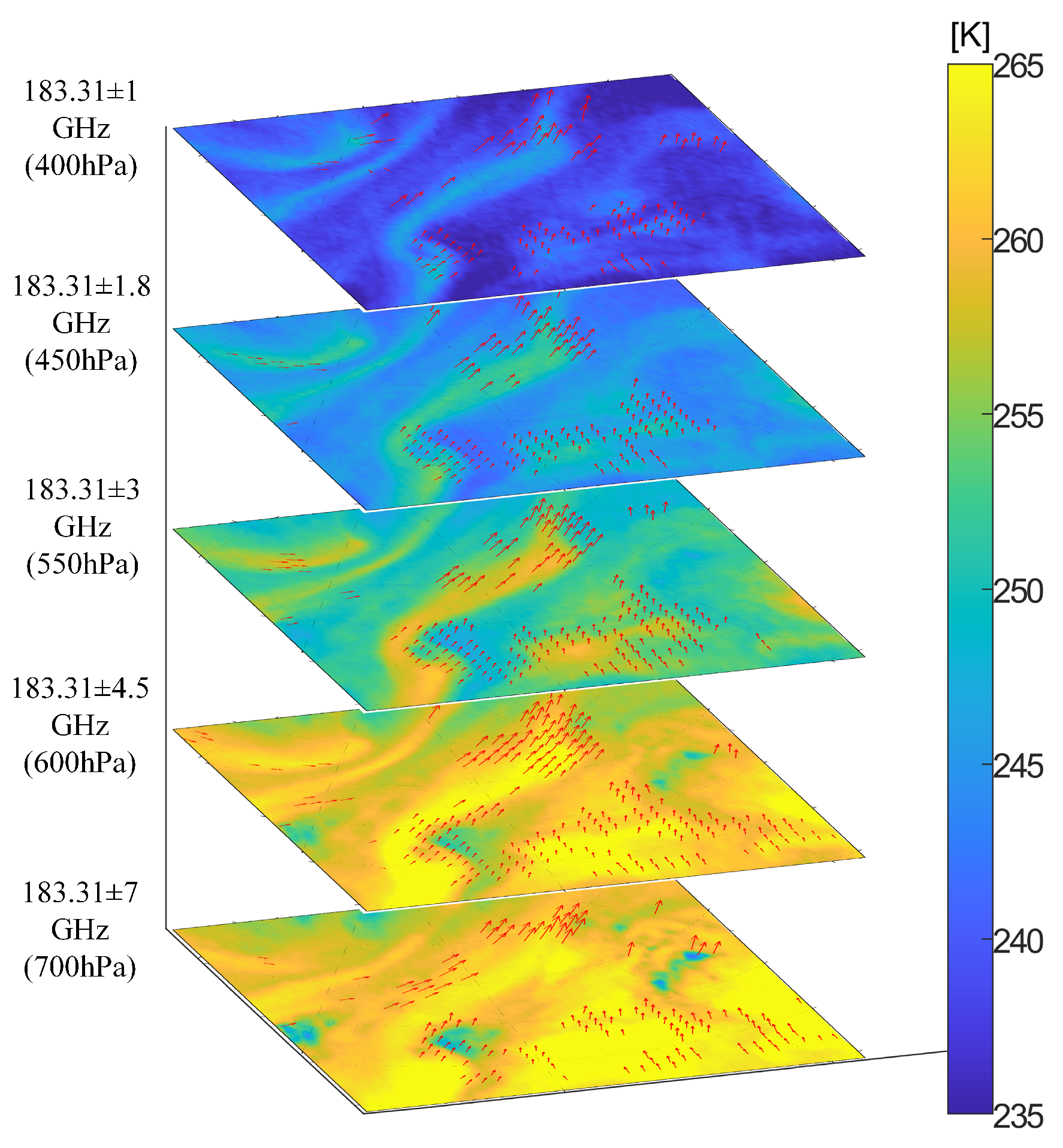
• The cloud dependence [13] for height assignment of AMV may be alleviated when using the five channels around the 183.31 GHz water-vapor absorption line.
• The temporal–spatial coverage of the polar wind record may be enriched by microwave radiometer data, especially considering that the Visible Infrared Imaging Radiometer Suite (VIIRS) lacks channels in either the infrared or the water-vapor absorption band for AMV derivation [14].
• Recent advancements in microwave radiometers aboard low-cost CubeSats constellations [15,16], as well as the concept of geostationary microwave sounders equipped with full-disk imaging capability via interferometric approaches [17,18,19,20], offer significant potential to facilitate the operational application of AMV-based wind records.

This study is devoted to substantiating the feasibility of AMV-based wind derived by passive microwave radiometers, using the realistic brightness temperature measured by the Micro-Wave Humidity Sounder-II (MWHS-II) onboard the FY-3D meteorological satellite [21]. A retrieval algorithm for water-vapor derived wind vectors is specifically developed, taking into account the polar orbit characteristics of the FY-3D satellite and the observational features of the MWHS-II.

2. Materials and Methods

2.1. Data

MWHS-II is one of the state-of-the-art total-power microwave radiometers onboard Chinese polar-orbiting meteorological satellites, and has fifteen channels in the range 89–191 GHz. The five channels centered at the 183.31 GHz water-vapor absorption line are selected to derive wind vectors, and the nominal spatial resolution is around 15 km at nadir. The Level-1 brightness temperature data are publicly accessible through the website of the National Satellite Meteorological Center (NSMC). For this study, we have collected and processed the entire dataset of 2022 in the Arctic region.

In situ measurements of wind field profiles are primarily obtained from radiosondes. However, the sparse distribution of measurement sites in polar regions poses challenges to obtaining comprehensive data. To address this limitation, the U/V components of wind from the ERA5 reanalysis dataset have been gathered as a reference for assessing retrieval quality in our study. The U-component represents the eastward component of the wind, indicating the horizontal speed of air moving towards the east. Conversely, the V-component represents the northward component of the wind, indicating the horizontal speed of air moving towards the north. Additionally, the dataset of NOAA JPSS VIIRS Level-3 Polar Winds is collected for a comparative analysis.

2.2. Method Overview

The AMV method employed in this study is designed based on the procedures that have been utilized to produce operational AMV wind records using optical sensors [22]. Due to the coarser spatial resolution of microwave radiometers compared to optical sensors, image triplets are utilized for feature tracking to ensure retrieval performance. Specifically, every three consecutive brightness temperature images are collected in high-latitude coverage up to 60 degrees poleward, resulting in a temporal span of 200 min. In the following content, we present and discuss the detailed implementation and modifications made to accommodate MWHS-II data.

2.3. Data Preprocessing

2.3.1. Parallax Correction

When observing the water-vapor feature off-nadir, its actual position is often displaced from its nominal position, as it typically exists above ground level. This displacement leads to what is commonly referred to as parallax [11]. To account for this effect, parallax correction is conducted for each channel separately with the satellite viewing geometry and the height assigned.

2.3.2. Remapping

Since the image triplets of interest overlap in the Arctic region, the brightness temperature data are remapped to a polar stereographic projection, avoiding the image distortion caused by map projection.

2.3.3. Resampling

Spatial resolution contributes to increased accuracy in the derived wind fields [23]. However, the spatial resolution of MWHS-II—183.31 GHz—is about 15 km, which is lower compared to MODIS—11 $\mathsf{\mu }$m (2 km)—and VIIRS—10.8 $\mathsf{\mu }$m (750 m)—channels. For a better water-vapor feature identification while preserving the image fidelity, the remapped brightness temperature data are resampled to a standard 5 km grid by two-dimensional interpolation.

2.3.4. Overlapping Location

The overlapped area of every three consecutive images is located from the resampled data, as illustrated in Figure 1. After applying the aforementioned preprocessing procedures, the resulting image triplets for wind tracking typically have a size of 2801 × 2801 pixels.

2.4. Target Selection

Given the sensitivity of the 183.31 GHz channels to water vapor, water vapor’s presence can be detected in brightness temperature images. To identify suitable targets, it is important to consider their variability, which can be automatically assessed using the local standard deviation (LSD) as follows. The LSD method has been validated in AVHRR wind records [24]. The selected target is shown in Figure 2a.

• Calculate the LSD of each pixel in the entire image within a 3 × 3 pixel area.
• Compute the cumulative distribution function of the LSD and determine the threshold at which the cumulative distribution function exceeds 0.9.
• Referencing EUMETAT’s target box size criteria [22] and through multiple experiments, the target box size was ultimately set to a size of 25 × 25 pixels. Within the target box, examine whether the local standard deviation of each pixel exceeds the threshold. If there are more than 5 pixels with a local standard deviation higher than the threshold, select that region as the target area.

2.5. Wind Tracking

After conducting target selection on the middle image of the image triplets, a wind tracking method based on cross-correlation is applied to the two consecutive image pairs. It is assumed that the targeted feature will not undergo significant movement within the 200 min time period. A search box with size of 130 × 130 pixels is created in the first and last images, centered on the selected target, ensuring that the maximum wind speed that can be tracked is 45 m/s. The cross-correlation is then calculated between the target area and the tracking area of the same size. The target tracking process is considered complete when the maximum correlation values in both the first and last images simultaneously exceed 0.9, indicating a strong correlation between the target and tracking areas. Subsequently, the wind vector is determined by averaging the two motion vectors from the consecutive image pairs. This average vector is assigned to the moment represented in the middle image. The described process is illustrated in Figure 2 for clarity and understanding.

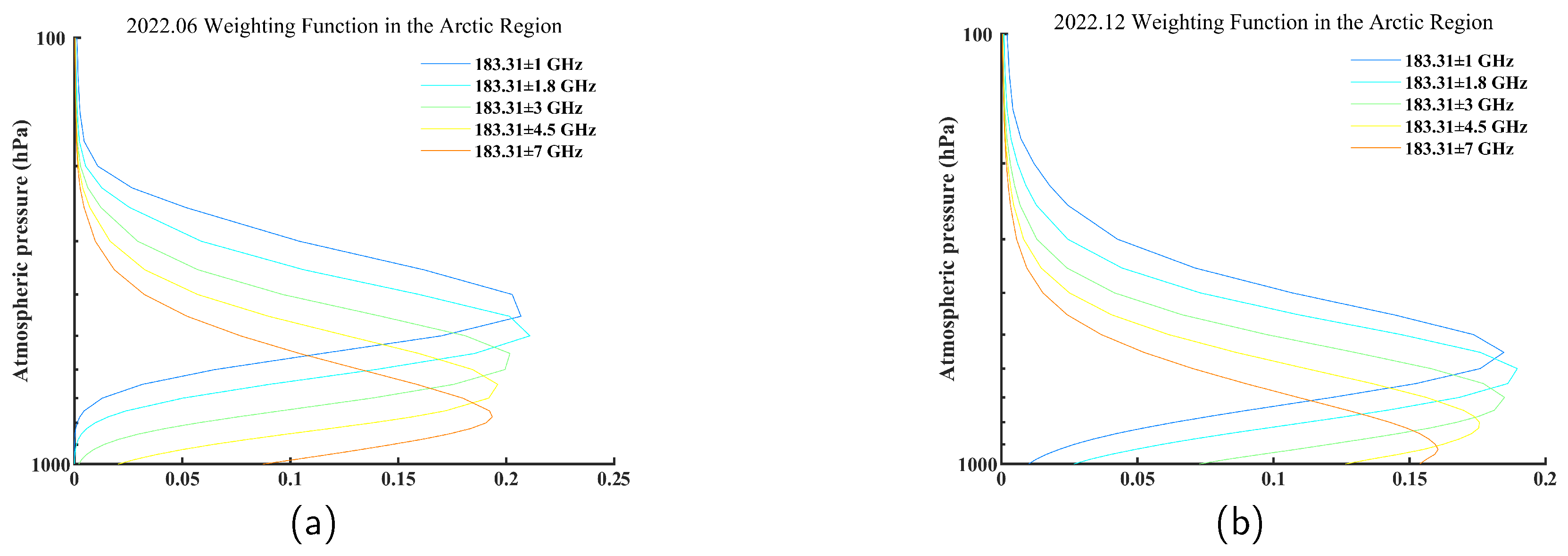
2.6. Height Assignment

Height assignment is recognized as one of the primary sources of error in AMV-based wind records. Sophisticated height assignment methods have been developed and implemented for visible and infrared data [25]. These methods typically rely on the forecast temperature profiles or simultaneous multi-spectral measurements.

Based on the model simulation of passive microwave observation for AMV-based wind derivation conducted by Zhang [26], using weighting function peak for the height assignment of each water-vapor channel around 183.31 GHz reveals promising results. However, it is important to consider that the atmospheric conditions in the Arctic region differ from those in tropical and mid-latitude regions. Thus, the monthly weighting function peak of each channel is recalculated using the atmospheric profiles from ERA5 monthly averaged reanalysis data, as presented in Figure 3 and

Table 1. MWHS-II water-vapor channels and monthly weighting function peaks.

Channel (GHz)		Weighting Function Peak (hPa)
		Jan.	Feb.	Mar.	Apr.	May	Jun.	Jul.	Aug.	Sep.	Oct.	Nov.	Dec.
183.31 ± 1.0		550	600	550	550	500	450	400	400	450	500	550	550
183.31 ± 1.8		600	650	650	600	550	500	450	450	500	550	600	600
183.31 ± 3.0		700	750	700	700	650	550	550	550	600	650	700	700
183.31 ± 4.5		825	825	825	800	750	650	600	650	650	750	800	800
183.31 ± 7.0		900	925	925	900	825	775	750	750	775	875	900	925

. This ensures that the height assignment for the derived wind vector is tailored to the specific atmospheric conditions prevailing in the corresponding month.

2.7. Quality Control

The European Organisation for the Exploitation of Meteorological Satellites (EUMETSAT) has developed a statistically based quality indicator (QI) for the operational AMV-based wind record [27]. In this study, we adopt a simplified version of the QI for the baseline automatic quality control test. It incorporates four consistency checks for speed, direction, vector, and spatial aspects. However, the forecast check is omitted to facilitate a smoother deployment. At the end of each AMV derivation cycle, the final QI is calculated as a weighted mean of the results from these four tests.

3. Results and Discussion

Since a specific monthly-dependent pressure height has been assigned to each channel, the retrieved wind vectors can be interpreted as a five-layer record. A typical illustration is presented in Figure 4. Quality evaluation is performed through a comparison with ERA5 reanalysis data and the VIIRS polar winds record. Statistical metrics, including the Pearson correlation coefficient (R), speed bias, direction bias, and vector root mean square error (RMSE), are calculated to assess the algorithm’s performance (definitions available in [28]). These four indicators are computed from the following:

$$\begin{array}{cc}\hfill R& =\frac{cov(Spee{d}_{\mathrm{MWHS}},Spee{d}_{\mathrm{ERA}5})}{{\sigma }_{Spee{d}_{\mathrm{MWHS}}}·{\sigma }_{Spee{d}_{\mathrm{ERA}5}}}\hfill \\ \hfill SpeedBias& =E(Spee{d}_{\mathrm{MWHS}}-Spee{d}_{\mathrm{ERA}5})\hfill \\ \hfill DirectionBias& =E(Directio{n}_{\mathrm{MWHS}}-Directio{n}_{\mathrm{ERA}5})\hfill \\ \hfill VectorRMSE& =\sqrt{E^2\left(SpeedDiff\right)+{\sigma }_{SpeedDiff}^2}\hfill \end{array}$$

(1)

where

$$SpeedDiff=\sqrt{{(u_{\mathrm{MWHS}}-u_{\mathrm{ERA}5})}^2+{(v_{\mathrm{MWHS}}-v_{\mathrm{ERA}5})}^2}$$

(2)

$$\begin{array}{cc}\hfill u_{\mathrm{MWHS}}& =\mathrm{u}-\mathrm{component}\mathrm{of}\mathrm{MWHS}-\mathrm{II}\mathrm{wind}\hfill \\ \hfill v_{\mathrm{MWHS}}& =\mathrm{v}-\mathrm{component}\mathrm{of}\mathrm{MWHS}-\mathrm{II}\mathrm{wind}\hfill \\ \hfill u_{\mathrm{ERA}5}& =\mathrm{u}-\mathrm{component}\mathrm{of}\mathrm{the}\mathrm{reference}\mathrm{ERA}5\mathrm{wind}\hfill \\ \hfill v_{\mathrm{ERA}5}& =\mathrm{v}-\mathrm{component}\mathrm{of}\mathrm{the}\mathrm{reference}\mathrm{ERA}5\mathrm{wind}\hfill \end{array}$$

$cov$, E, and $\sigma$ represent covariance, expectation, and standard deviation.

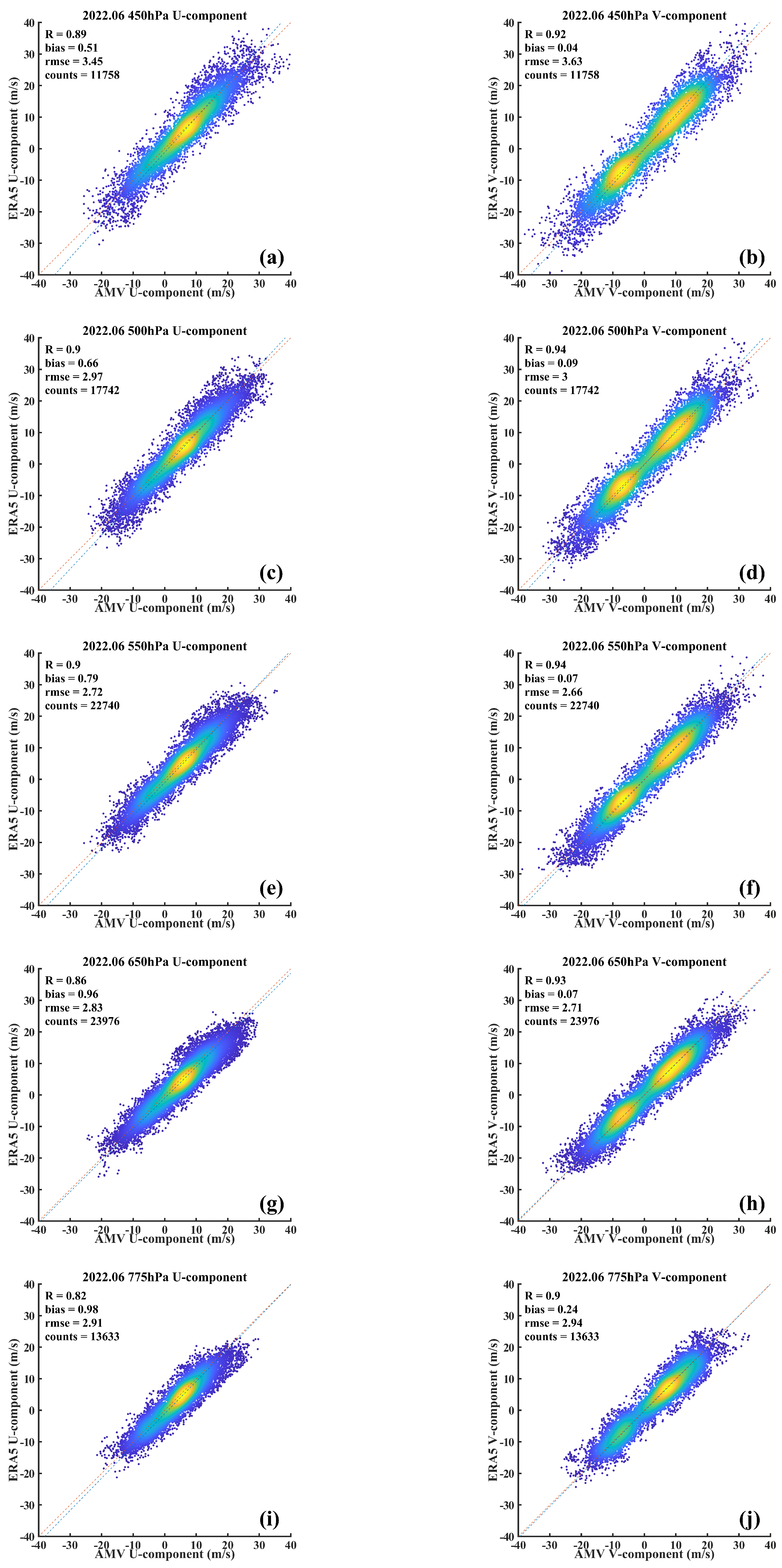
3.1. Seasonal Evaluation Using ERA5 Reanalysis Data

Quality evaluation employs the U/V wind components from ERA5 hourly data on pressure levels, with a comparison based on the nearest criterion in both temporal (1 h) and geospatial (${0.25}^{\circ }\times {0.25}^{\circ }$) domains. Considering that the water-vapor feature is highly dependent on seasonal variation, the evaluation results are categorized by seasons: Spring (months 3/4/5), Summer (months 6/7/8), Autumn (months 9/10/11), and Winter (months 12/1/2), as shown in

Table 2. Seasonal statistical metrics of FY-3D MWHS-II 183.31 GHz water-vapor winds in the Arctic region for 2022 (QI ≥ 0.8).

Channel (GHz)		Data Counts				Speed Bias (m/s)				Direction Bias (degree)				Vector RMSE (m/s)
		Spring	Summer	Autumn	Winter	Spring	Summer	Autumn	Winter	Spring	Summer	Autumn	Winter	Spring	Summer	Autumn	Winter
183.31 ± 1.0		14,203	33,845	12,669	10,496	−0.2	−0.7	−0.3	−0.2	3.1	1.4	3.0	4.1	5.4	5.2	5.7	5.9
183.31 ± 1.8		19,302	53,371	18,889	15,347	0.2	−0.2	−0.1	−0.2	3.2	0.8	2.9	2.2	4.9	4.3	5.1	5.2
183.31 ± 3.0		26,772	70,753	23,892	25,430	0.3	0.6	0.5	−0.2	1.7	0.6	3.6	0.1	4.4	3.9	4.6	4.5
183.31 ± 4.5		38,951	78,679	25,939	28,929	0.0	0.9	0.4	−0.4	1.0	1.1	2.8	−0.0	3.8	3.9	4.2	4.0
183.31 ± 7.0		30,783	49,192	18,700	17,578	−0.3	0.9	0.2	−0.2	1.4	1.8	2.8	2.3	3.7	4.2	4.1	4.1

.

It is found that the retrieved wind vector’s quality increases with lower assigned height levels, indicating atmospheric penetration capability. Spring and Summer exhibit more retrieved wind vectors that pass quality control, accompanied by improvements in statistical metrics. However, a minor quality deterioration is observed in the bottom layer across all seasons, potentially due to underlying surface influences.

For further insight into the retrieved wind vector’s quality, Figure 5 illustrates the comparison with ERA5 data for U/V components, focusing on June 2022. The blue dashed lines are fitting lines between the U/V components of MWHS-II wind vectors and the corresponding ERA5 U/V components. The red dashed lines represent the standard line of y = x. The U/V-component retrieval performance aligns with the results in Table 2. Quality control effectively filters out poor-quality retrievals, resulting in an overall correlation coefficient of nearly 0.9.

In summary, the proposed algorithm demonstrates the wind retrieval capability of MWHS-II 183.31 GHz channels in the Arctic region, exhibiting a subtle performance variation across seasons. Following moderate quality control (QI ≥ 0.8), wind vector RMSEs are approximately 4.5 m/s for the three lower-height channels and 5.5 m/s for the two upper-height channels, indicating promising retrieval quality.

3.2. Comparison with NOAA VIIRS Polar Winds Record

Presently, the state-of-the-art polar wind field record is provided by the VIIRS (10.8-$\mathsf{\mu }$m channel) aboard Suomi National Polar-orbiting Partnership (SNPP). To further assess the MWHS-II wind vector quality, a comparison is conducted with ERA5 data as the benchmark. Specifically, we examined their quality metrics against ERA5 for the same time period (June and December 2022), the same geographical region (Arctic), and the same quality control (QI ≥ 0.8). The geospatial and temporal matchup adheres to the nearest criterion. However, VIIRS wind height assignment is not ERA5-dependent and ranges from 100 hPa to 1000 hPa. We choose the five pressure levels assigned to MWHS-II winds for comparison and collect comparable VIIRS winds (within ±25 hPa) to calculate statistical metrics. The resulting comparisons of statistical metrics are presented in

Table 3. Comparison of MWHS-II and VIIRS winds in the Arctic region for June 2022 (QI ≥ 0.8).

Pressure (hPa)		Data Counts		Speed Bias (m/s)		Direction Bias (degree)		Vector RMSE (m/s)
		MWHS-II	VIIRS	MWHS-II	VIIRS	MWHS-II	VIIRS	MWHS-II	VIIRS
450		11,758	21,360	−0.5	0.6	1.9	−0.7	5.0	3.8
500		17,742	12,486	0.0	0.4	1.5	−0.7	4.2	3.4
550		22,740	7530	0.2	0.2	0.9	−0.5	3.8	3.2
650		23,976	4597	0.9	−0.1	1.5	0.1	3.9	3.1
775		13,633	4775	0.8	0.1	2.0	0.4	4.1	3.1

and

Table 4. Comparison of MWHS-II and VIIRS winds in the Arctic region for December 2022 (QI ≥ 0.8).

Pressure (hPa)		Data Counts		Speed Bias (m/s)		Direction Bias (degree)		Vector RMSE (m/s)
		MWHS-II	VIIRS	MWHS-II	VIIRS	MWHS-II	VIIRS	MWHS-II	VIIRS
550		3835	9492	−0.3	0.4	4.0	0.2	5.8	3.8
600		5212	5672	−0.1	0.2	2.5	0.0	5.0	3.7
700		7720	3442	0.0	0.0	0.7	0.6	4.5	3.6
800		8045	2336	−0.1	−0.2	0.1	0.1	4.1	3.6
925		5101	2995	−0.3	−0.2	2.0	−1.0	4.3	3.6

, respectively. The reason we present the results obtained in June and December is that June represents moister conditions, while December represents drier conditions. Following the two-month comparison with VIIRS winds, key features of MWHS-II winds can be summarized:

• Benefiting from cloud penetration capability, more wind vectors are retrieved at lower height levels, which forms an effective supplements to the existing cloud-dependent wind records.
• Quality metrics at lower height levels are comparable to the state-of-the-art VIIRS wind record, although upper height levels exhibit some deterioration, demonstrating an overall good retrieval quality. The residual speed bias and direction bias may be attributed to the inferior spatial resolution, and require further investigation.

Additionally, as presented in Figure 6, the spatial distribution and data count of AMVs for June 2022 is illustrated and compared between the VIIRS and MWHS-II data records. The data are gridded on a $1^{\circ }\times 1^{\circ }$ grid, the counts of AMVs are calculated for every grid point, and then the data are compared. The distribution of VIIRS AMVs exhibits a gradual decline from the upper to the lower atmosphere, whereas the presence of MWHS-II AMVs shows an increasing trend, particularly characterized by a rich amount of high-quality vectors in oceanic regions. This finding suggests a synergistic interplay between the MWHS-II and VIIRS AMVs. Notably, MWHS-II AMVs are promising in substantially enhancing the coverage of reliable AMVs in the lower atmospheric layers, with a marked emphasis on oceanic areas.

It is also important to note that 77% of VIIRS winds ranging from 450 to 775 hPa are included in the comparison presented in Table 3, and 71% ranging from 550 to 925 hPa for Table 4. The cloud dependence of VIIRS winds facilitates higher data availability at upper height levels, while the deficiency at lower height levels can be reasonably supplemented by MWHS-II (or other passive microwave sensors) wind products.

4. Conclusions

This study presents an AMV-based water-vapor wind retrieval method for passive microwave radiometers, marking the first attempt to utilize 183.31 GHz MWHS-II brightness temperature data for generating wind vector records in the Arctic region. The method’s validity has been demonstrated through the assessment of statistical metrics using ERA5 hourly data on pressure levels and operational VIIRS polar wind records for the entire year of 2022.

Although applying a monthly-dependent height assignment, the vector RMSEs are approximately 4.5 m/s for the three lower-height channels and 5.5 m/s for the two upper-height channels. The presented preliminary retrieval performance can be further enhanced by incorporating forecast data into the quality control process. These findings indicate a retrieval quality comparable to VIIRS winds. Owing to the cloud penetration capability at the microwave band, the AMV-based wind data derived from 183.31 GHz brightness temperatures show potential for augmenting data availability at lower height levels through careful operational product development. Furthermore, the results hold promise for supporting future applications of the evolving passive microwave satellite program, whether in the context of geostationary satellites or CubeSats constellations.

References

1. National Research Council. Earth Science and Applications from Space: National Imperatives for the Next Decade and Beyond; The National Academies Press: Washington, DC, USA, 2007. [Google Scholar]
2. Zeng, X.; Ackerman, S.; Ferraro, R.D.; Lee, T.J.; Murray, J.J.; Pawson, S.; Reynolds, C.; Teixeira, J. Challenges and opportunities in NASA weather research. Bull. Am. Meteorol. Soc. 2016, 97, ES137–ES140. [Google Scholar] [CrossRef]
3. Schmetz, J.; Holmlund, K.; Hoffman, J.; Strauss, B.; Mason, B.; Gaertner, V.; Koch, A.; Van De Berg, L. Operational cloud-motion winds from Meteosat infrared images. J. Appl. Meteorol. Climatol. 1993, 32, 1206–1225. [Google Scholar] [CrossRef]
4. Forsythe, M.; Peubey, C.; Lupu, C.; Cotton, J. Assimilation of wind information from radiances: AMVs and 4D-Var tracing. In Proceedings of the ECMWF Annual Seminar, Grande Prairie, AB, Canada, 8–12 September 2014. [Google Scholar]
5. Izawa, T.; Fujita, T. Relationship between Winds and Cloud Velocities Determined from Pictures Obtained by the ESSA 3, ESSA 5 and AST-I Satellites; North-Hol land Publishing Co., Space Research IX: Amsterdam, The Netherlands, 1969; pp. 571–579. [Google Scholar]
6. Fujita, T.T. Principle of stereoscopic height computations and their applications to stratospheric cirrus over severe thunderstorms. J. Meteorol. Soc. Jpn. Ser. II 1982, 60, 355–368. [Google Scholar] [CrossRef]
7. Menzel, W.P. Cloud tracking with satellite imagery: From the pioneering work of Ted Fujita to the present. Bull. Am. Meteorol. Soc. 2001, 82, 33–48. [Google Scholar] [CrossRef]
8. Nieman, S.J.; Menzei, W.P.; Hayden, C.M.; Gray, D.; Wanzong, S.T.; Velden, C.S.; Daniels, J. Fully automated cloud-drift winds in NESDIS operations. Bull. Am. Meteorol. Soc. 1997, 78, 1121–1134. [Google Scholar] [CrossRef]
9. Bresky, W.C.; Daniels, J.M.; Bailey, A.A.; Wanzong, S.T. New methods toward minimizing the slow speed bias associated with atmospheric motion vectors. J. Appl. Meteorol. Climatol. 2012, 51, 2137–2151. [Google Scholar] [CrossRef]
10. Herman, L. High frequency satellite cloud motion at high latitudes. In Proceedings of the Symposium on Meteorological Observations and Instrumentation, Anaheim, CA, USA, 17–22 January 1993; pp. 465–468. [Google Scholar]
11. Key, J.R.; Santek, D.; Velden, C.S.; Bormann, N.; Thepaut, J.N.; Riishojgaard, L.P.; Zhu, Y.; Menzel, W.P. Cloud-drift and water vapor winds in the polar regions from MODIS. IEEE Trans. Geosci. Remote Sens. 2003, 41, 482–492. [Google Scholar] [CrossRef]
12. Lambrigtsen, B.; Van Dang, H.; Turk, F.J.; Hristova-Veleva, S.M.; Su, H.; Wen, Y. All-weather tropospheric 3-D wind from microwave sounders. IEEE J. Sel. Top. Appl. Earth Obs. Remote Sens. 2018, 11, 1949–1956. [Google Scholar] [CrossRef]
13. Eyre, J.R.; Bell, W.; Cotton, J.; English, S.J.; Forsythe, M.; Healy, S.B.; Pavelin, E.G. Assimilation of satellite data in numerical weather prediction. Part II: Recent years. Q. J. R. Meteorol. Soc. 2022, 148, 521–556. [Google Scholar] [CrossRef]
14. Santek, D.; Nebuda, S.; Stettner, D. Demonstration and evaluation of 3D winds generated by tracking features in moisture and ozone fields derived from AIRS sounding retrievals. Remote Sens. 2019, 11, 2597. [Google Scholar] [CrossRef]
15. Blackwell, W.J.; Braun, S.; Bennartz, R.; Velden, C.; DeMaria, M.; Atlas, R.; Dunion, J.; Marks, F.; Rogers, R.; Annane, B.; et al. An overview of the TROPICS NASA earth venture mission. Q. J. R. Meteorol. Soc. 2018, 144, 16–26. [Google Scholar] [CrossRef] [PubMed]
16. Goncharenko, Y.V.; Berg, W.; Reising, S.C.; Iturbide-Sanchez, F.; Chandrasekar, V. Design and Analysis of CubeSat Microwave Radiometer Constellations to Observe Temporal Variability of the Atmosphere. IEEE J. Sel. Top. Appl. Earth Obs. Remote Sens. 2021, 14, 11728–11736. [Google Scholar] [CrossRef]
17. Zhang, C.; Liu, H.; Wu, J.; Zhang, S.; Yan, J.; Niu, L.; Sun, W.; Li, H. Imaging Analysis and First Results of the Geostationary Interferometric Microwave Sounder Demonstrator. IEEE Trans. Geosci. Remote Sens. 2015, 53, 207–218. [Google Scholar] [CrossRef]
18. Duruisseau, F.; Chambon, P.; Guedj, S.; Guidard, V.; Fourrié, N.; Taillefer, F.; Brousseau, P.; Mahfouf, J.F.; Roca, R. Investigating the potential benefit to a mesoscale NWP model of a microwave sounder on board a geostationary satellite. Q. J. R. Meteorol. Soc. 2017, 143, 2104–2115. [Google Scholar] [CrossRef]
19. Guo, X.; Liu, H.; Niu, L.; Zhang, C.; Lu, H.; Huo, C.; Wang, T.; Wu, J. Data Processing and Experimental Performance of GIMS-II (Geostationary Interferometric Microwave Sounder-Second Generation) Demonstrator. In Proceedings of the 2018 IEEE 15th Specialist Meeting on Microwave Radiometry and Remote Sensing of the Environment (MicroRad), Cambridge, MA, USA, 27–30 March 2018; pp. 1–4. [Google Scholar] [CrossRef]
20. Lambrigtsen, B.; Kangaslahti, P.; Montes, O.; Niamsuwan, N.; Posselt, D.; Roman, J.; Schreier, M.; Tanner, A.; Wu, L.; Yanovsky, I. A Geostationary Microwave Sounder: Design, Implementation and Performance. IEEE J. Sel. Top. Appl. Earth Obs. Remote Sens. 2022, 15, 623–640. [Google Scholar] [CrossRef]
21. Guo, Y.; He, J.; Gu, S.; Lu, N. Calibration and Validation of Feng Yun-3-D Microwave Humidity Sounder II. IEEE Geosci. Remote Sens. Lett. 2020, 17, 1846–1850. [Google Scholar] [CrossRef]
22. Borde, R.; Hautecoeur, O.; Carranza, M. EUMETSAT global AVHRR wind product. J. Atmos. Ocean. Technol. 2016, 33, 429–438. [Google Scholar] [CrossRef]
23. Velden, C.S.; Stettner, D.; Daniels, J. Wind vector fields derived from GOES rapid-scan imagery. In Proceedings of the 10th Conference on Satellite Meteorology and Oceanography, Long Beach, CA, USA, 9 January 2000; pp. 20–23. [Google Scholar]
24. Borde, R.; Doutriaux-Boucher, M.; Dew, G.; Carranza, M. A direct link between feature tracking and height assignment of operational EUMETSAT atmospheric motion vectors. J. Atmos. Ocean. Technol. 2014, 31, 33–46. [Google Scholar] [CrossRef]
25. Salonen, K.; Cotton, J.; Bormann, N.; Forsythe, M. Characterizing AMV Height-Assignment Error by Comparing Best-Fit Pressure Statistics from the Met Office and ECMWF Data Assimilation Systems. J. Appl. Meteorol. Climatol. 2015, 54, 225–242. [Google Scholar] [CrossRef]
26. Zhang, Y.; Hu, H.; Weng, F. The Potential of Satellite Sounding Observations for Deriving Atmospheric Wind in All-Weather Conditions. Remote Sens. 2021, 13, 2947. [Google Scholar] [CrossRef]
27. Holmlund, K. The utilization of statistical properties of satellite-derived atmospheric motion vectors to derive quality indicators. Weather. Forecast. 1998, 13, 1093–1104. [Google Scholar] [CrossRef]
28. Santek, D. The Global Impact of Satellite-Derived Polar Winds on Model Forecasts. Ph.D. Thesis, University of Wisconsin–Madison, Madison, WI, USA, 2007. [Google Scholar]
Figure 1. Sample overlapping areas from which MWHS-II AMV-based winds are extracted in image triplets.
Remotesensing 16 01715 g001
Figure 2. Illustration of AMV-based wind tracking process. (a) The target box selected following the process described in Section 2.4. (b) The target box tracked in the next image following the process described in Section 2.5.
Remotesensing 16 01715 g002
Figure 3. The weighting functions of the five water-vapor channels: (a) June 2022, (b) December 2022.
Remotesensing 16 01715 g003
Figure 4. Sample retrieved wind fields and brightness temperatures in the region 70°N to 90°N, 135°W to 150°E at 19:28:00 UTC, 3 July 2022.
Remotesensing 16 01715 g004
Figure 5. Scatterplots of the retrieved MWHS-II winds in U (left column) and V (right column) components compared with ERA5 data in the Arctic region for June 2022: (a,b) 183 ± 1 GHz (400 hPa), (c,d) 183 ± 1.8 GHz (450 hPa), (e,f) 183 ± 3 GHz (550 hPa), (g,h) 183 ± 4.5 GHz (600 hPa), (i,j) represents 183 ± 7 GHz (750 hPa). Regions with a more yellow hue represent areas of higher data density, while regions with a more blue hue indicate areas of lower data density.
Remotesensing 16 01715 g005
Figure 6. Spatial distribution and data count of (a) VIIRS and (b) MWHS-II AMVs in June 2022.
Remotesensing 16 01715 g006