Article

Fault Detection and Interactive Multiple Models Optimization Algorithm Based on Factor Graph Navigation System

1
School of College of Automation and Control, Nanjing University of Aeronautics and Astronautics, Nanjing 211106, China
2
Jiangsu University Collaborative Innovation Center for Satellite Communication and Navigation, Nanjing 211106, China
*
Author to whom correspondence should be addressed.
Remote Sens. 2024, 16(10), 1651; https://doi.org/10.3390/rs16101651
Submission received: 1 March 2024 / Revised: 22 April 2024 / Accepted: 5 May 2024 / Published: 7 May 2024
(This article belongs to the Section Engineering Remote Sensing)

Abstract

:
Accurate and stable positioning is significant for vehicle navigation systems, especially in complex urban environments. However, urban canyons and dynamic interference make vehicle sensors prone to disturbance, leading to vehicle positioning errors and even failures. To address these issues, an adaptive loosely coupled IMU/GNSS/LiDAR integrated navigation system based on factor graph optimization with sensor weight optimization and fault detection is proposed. First, the factor nodes and system framework are constructed based on error models of sensors, and the optimization method principle is derived. Second, the interactive multiple-model algorithm based on factor graph optimization (IMMFGO) is utilized to calculate and adjust sensor weights for global optimization, which will reduce the impact of disturbed sensors. Finally, a multi-stage fault detection, isolation, and recovery (MSFDIR) strategy is implemented based on the IMMFGO results and IMU pre-integration measurements, which can detect significant sensor faults and optimize the system structure. Vehicle experiments show that our IMMFGO method generally obtains better performance in positioning accuracy by 23.7% compared to adaptive factor graph optimization (AFGO) methods, and the MSFDIR strategy possesses the capability of fault sensor detection, which provides an essential reference for multi-source vehicle navigation systems in urban canyons.

1. Introduction

Effective positioning and navigation are vital for autonomous systems, such as unmanned driving and intelligent vehicles, especially in complex urban environments [1,2,3]. The realization of autonomous transportation systems depends on multi-sensor information fusion from the inertial measurement unit (IMU), global navigation satellite system (GNSS), and vision sensor measurements [4]. However, due to the disturbance caused by complex environments, vehicle sensors are prone to significant errors and even failures [5]. An inertial navigation system (INS) is a good choice for urban positioning because of its short-time high precision characteristic. Nevertheless, the errors in INS measurements will accumulate over time and may have a sudden increase affected by the fluctuation or vibration of the transport systems without auxiliary sensors [6]. GNSS has the ability to provide high-precision navigation information and compensates for the accumulation of INS errors through an integrated navigation scheme, but its signals are susceptible to external environmental influence [7]. Affected by occlusion from complex environments, such as high-rise buildings and tunnels, GNSS may become completely ineffective. Therefore, the urban environment has a significant impact on the navigation accuracy of GNSS [8]. Visual navigation systems have attracted significant attention in autonomous systems, and LiDAR is widely used due to its high precision and high-frequency data acquisition capability. LiDAR alone for navigation may be difficult due to the loss of features or the insensitivity to dynamic targets in urban environments [9]. Considering the disturbance under complex urban environments, an effective fault detection and adaptive integrated navigation method is necessary for vehicle safety.
Integrated navigation schemes based on multi-source information fusion for vehicle navigation have been extensively investigated. Considering the difficulties of accurate modeling and prediction for external dynamic disturbance, the traditional extended Kalman filter (EKF) algorithm fails to satisfy the robustness requirements [10,11]. To address this problem, the adaptive Kalman filter (AKF) provides a solution. Shen et al. introduced an improved multi-rate strong tracking cubature Kalman filter (CKF) to estimate the system covariance adaptively [12]. Also, a dual optimization scheme comprising a CKF-multiple layer perceptron and radial basis function-CKF was proposed to maintain system accuracy during GNSS denying [13]. The factor graph algorithm is featured due to its multi-source asynchronous information fusion and plug-and-play abilities. It has been widely applied in navigation and simultaneous localization and mapping (SLAM) areas for data optimization [14]. As a probability graph model, the factor graph is able to estimate and update the state variables through graph modeling of mathematical problems. A direct method for navigation is constructing the multi-source navigation system under factor graph modeling and using graph optimization as a filter for information fusion. Indelman proposed an inertial/visual integrated navigation system which describes sensor error models of factor nodes and estimates the system states through the factor graph optimization algorithm [15]. To verify the effectiveness of the factor graph model, Xu. et al. compared the factor graph algorithm with EKF using dataset experiments. The results showed that as an information fusion strategy, the factor graph performs better in disturbed environments owing to its historical information fusion ability [16]. Additionally, the sliding window algorithm enables the factor graph to marginalize information, thus reducing the computational burden of the whole system and improving the real-time performance. Another application of factor graphs is solving the SLAM backend optimization problem. SLAM has a strong ability to establish the model of the surrounding environment by applying visual sensors, which is a complementary strategy for GNSS disturbance scenes [17]. Nevertheless, SLAM has limitations for weak characteristic environments, such as piping and tubes, resulting in error accumulation and scene degradation [18]. The collaborative navigation method is a feasible solution. Through the collaboration constraints measured by multi-robots, the state can be updated based on pose constraint factors and achieve high positioning accuracy [19]. Regarding favorable environment estimation, Chen et al. constructed a prior map by LiDAR to assist in estimating an inertial/GNSS tight-coupled navigation system when GNSS is in good condition. The scene optimizer and sliding window also improve the system’s performance [20]. Therefore, the factor graph algorithm can satisfy the multi-source asynchronous fusion function and improve the comprehensive system’s performance in various conditions. Nevertheless, it is still inevitable that the system suffers from sensor failure, which significantly reduces the navigation accuracy of the global system.
With the increasing number and variety of sensors in vehicle navigation systems, the possibility of sensor faults is also increasing, resulting in poor system estimation and positioning accuracy. Fault detection, isolation, and recovery (FDIR) methods, which generally obtain system state and identify faults to isolate or restore sensors by determining whether the index of sensor measurements exceeds the target threshold, become significant to the system reliability and safety [21,22,23]. The residual chi-square statistical method is typically applied in navigation fault detection system, and the detection function is constructed to calculate the index through Kalman filter (KF) method, which detects the positioning faults of sensors based on the prediction information and determines whether a fault exists [24]. Wang et al. constructed the IMU/GNSS tightly coupled system based on EKF and detected the system faults with the assistance of LiDAR real-time estimation [25]. In urban areas, GNSS signals may suffer from the multipath effect or non-line-of-sight (NLOS) signal interference due to reflections, and the whole system tends to provide poor positioning results. The pseudo-range errors are well calculated and account for signal strength, satellite elevation angle, and coordinate information. These algorithms have been developed based on the KF algorithm under the assumption that GNSS measurements come with Gaussian uncorrelated white noise. But the existence of colored noise in GNSS measurements, typical for positioning with low-cost GNSS receivers, will degrade the performance of KF-based fault detection and exclusion (FDE) algorithms. To obtain more accurate estimation results, Gao et al. proposed an improved considering colored noise model to improve the FDE performance [26]. However, satellites still suffer from multipath signals, and the error model cannot be constructed. Multiple model adaptive estimation (MMAE) provides a feasible solution to avoid directly estimating unknown faults. Considering that the dynamic model of the localization is highly nonlinear, Kheirandish et al. provided the navigation strategy of fusing multi-sensor measurements with an interactive multiple model (IMM) algorithm based on unscented Kalman filters (UKF) and EKF [27]. Xiong et al. proposed a hybrid robust Gaussian belief propagation method as a cooperative positioning system for transportation navigation, which applies an IMM structure to fuse FDE with Huber’s M-estimation method and combines the advantages of both without drawbacks [28]. Given the decline in estimation and diagnostic accuracy caused by the fixed transformation probability models of IMM, Wang et al. combined an adaptive interacting multiple model filter and federated Kalman algorithm to achieve an outlier detection function [29]. All of the above algorithms are suitable for the FDE of vehicle navigation systems in complex urban environments. However, the systems are mainly constructed using KF, EKF, and UKF filters, and the structure is challenging to change adaptively for sensor isolation and recovery [30]. Therefore, building a flexible system structure with multi-sensors is necessary to adapt to different scenarios.
In this paper, a multi-source integrated navigation system with interactive multiple models based on factor graph optimization and multi-stage fault detection, isolation, and recovery functions for urban positioning is proposed to deal with the existing problems. On the one hand, the IMU/GNSS/LiDAR factor graph navigation system is constructed, and the bias of IMU pre-integration is estimated and corrected by GNSS pseudo-range difference measurements and LiDAR iterative closest point (ICP) measurements [31]. Therefore, multi-source asynchronous sensors are fused based on the high-frequency IMU integration by factor graph optimization. Then, the sliding window algorithm is applied to marginalize the historical information and guarantee the real-time performance of the whole system [32]. On the other hand, the location-level interactive multiple models algorithm based on factor graph optimization (IMMFGO) of GNSS and LiDAR is performed to update sensor weights in global optimization. The multi-stage fault detection, isolation, and recovery (MSFDIR) method is applied to reduce the impact of fault measurement and to adaptively optimize system structures. Vehicle experiments with adequate analysis have verified the accuracy and efficiency of the proposed method, which can realize good performance for positioning and fault detection for vehicle navigation in urban canyons. The main contributions of this paper are as follows:
  • An IMU/GNSS/LiDAR integrated navigation system framework based on factor graph optimization is constructed. Meanwhile, the error models of sensors are constructed in a formulaic factor graph optimization system, and the ISAM2 sliding window algorithm is applied to marginalize the historical information and improve the real-time performance.
  • The IMMFGO algorithm of GNSS and LiDAR sub-model measurements is applied to update the weights of the sensors in global optimization. The MSFDIR strategy is employed to detect, isolate and restore fault sensors and reconstruct the system frameworks to adapt to external disturbances.
  • Vehicle experiments are conducted to verify the effectiveness of the proposed methods. Qualitative and quantitative analyses are applied to comprehensively compare the performance of proposed IMMFGO and MSFDIR with other typical algorithms to demonstrate the superiority of the proposed method and the possibility of application in natural vehicle navigation systems.

2. System Structures

2.1. System Solution

The overview of the proposed framework is described in Figure 1, which is a loosely coupled IMU/GNSS/LiDAR integrated navigation system based on factor graph optimization. The main structure of the system is constructed by IMU measurements, while GNSS and LiDAR provide auxiliary information to correct state variables.
The navigation system can be divided into three parts: (1) Factor construction: the IMU pre-integration factors and IMU bias factors are constructed based on IMU measurements, and the pseudo-range difference algorithm and iterative closest point algorithm (ICP) are applied to deal with GNSS and LiDAR measurements. (2) Nonlinear optimization: the factor graph framework is constructed based on modelled factors, and the ISAM2 sliding window algorithm is applied for filtering. The proposed IMMFGO algorithm can change the weights of corresponding sensors to achieve an adaptive optimization function. The IMMFGO includes parts of the input interactions of models, smoothing and fusion of models, and probability update of models, while the system will finally output the navigation states. (3) Multi-stage fault detection, isolation, and recovery: the results of IMMFGO and the navigation state will be used for system fault detection, isolation, and recovery. The system will detect faults based on the results of IMMFGO and IMU pre-integration measurements, respectively. The detection results determine whether to isolate or restore the fault sensor, and the factor graph navigation framework will be reconstructed on time. The frames and the notations used in the system are defined as follows:
  • The coordinate of IMU is defined as { } B , which is set at the center of the IMU sensor and is the same as the body-fixed coordinate;
  • The GNSS frame is defined as { } G , which is set as the WGS-84 coordinate, and the measurement of GNSS is transferred into a navigation coordinate by the transform matrix R G W ;
  • The LiDAR frame is defined as { } L , which is set at the center of the LiDAR sensor, and the transform matrix from the LiDAR coordinate into the navigation coordinate is R L W ;
  • The world frame is the ENU frame and is defined as { } W , which is set at the initial position of the vehicle and is assumed to coincide with the initial LiDAR frame.

2.2. Factor Graph Structure

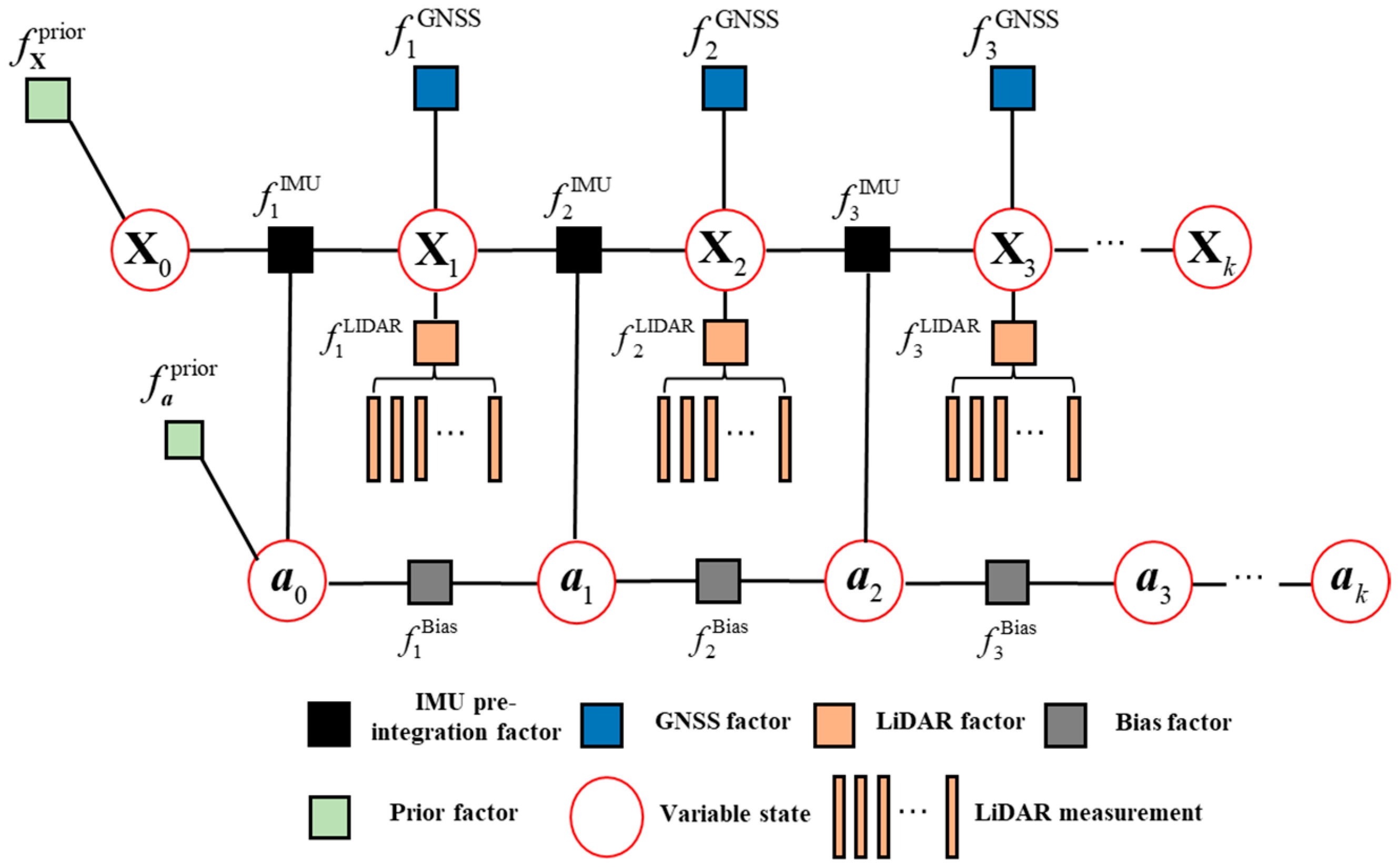
The factor graph optimization approach has the characteristics of plug-and-play and historical information fusion. The ability of multi-source asynchronous data fusion makes factor graphs more reliable and robust than the EKF [33]. Therefore, the IMU/GNSS/LiDAR factor graph integrated system for vehicle navigation is constructed to estimate the navigation state in complex urban areas, which applies the ISAM2 sliding window algorithm to ensure real-time performance and accuracy. The structure of the factor graph system is shown in Figure 2.
As shown in Figure 2, the system is estimated by fusing information from IMU pre-integration factors, LiDAR factors, and GNSS factors and introducing five types of factors to construct the whole framework. The information fusion frequency is based on the lowest frequency sensor, which is set as the GNSS frequency in this paper. The factor graph G = ( F l , X m , E n ) is a probabilistic graphical model (PGM) and mainly includes two kinds of nodes with edges connecting between them [34]. The factor node f i F l represents the measurement information from the sensors, and the variable node x j X m represents the state information to estimate the navigation state. The system is constructed by the factor nodes, with variable nodes connecting them by edges e i j E n . The definition and the structure of the nodes are illustrated in Section 2.3 and Section 2.4.
Since the northeast up coordinate system is set as the navigation system, the system navigation state and the variable nodes at time k can be defined as follows:
X k = [ p k W , v k W , q k W , b a k , b g k ] T
where the first three parameters are information from each sensor measurement. p k W includes the p E , p N , p U position results, v k W includes the v E , v N , v U velocity results, and q k W includes the q E , q N , q U platform rotation. b a k and b g k are accelerometer bias and gyroscope bias, respectively, including slowly changing bias and random noise bias.
According to the state estimation and the factor graph mathematical model principle, the factor graph optimization method is typically derived as a nonlinear least-squares problem [35]. Assuming that the system model follows the Gaussian noise distributions, the factor edges can be defined as follows:
f i ( X k ) exp ( 1 2 h k i ( X k ) Z k Σ i 2 )
where i indicates the type of sensor, h k i ( ) represents the nonlinear measurement function, Z k represents the actual measurements of the sensors, and i represents the covariance matrix. The factor graph estimates the system state by solving the maximum a posteriori (MAP) probability of the probability distribution function (PDF) [36]. Through the transformation of the MAP formula, it can be defined as follows:
X k = arg min I h k i ( X k ) Z k i 2
where X k represents the global optimal solution. To solve the nonlinear least squares problems, we generally apply the first-order Taylor expansion formula to linearize the function and use the Gaussian Newton method or Levenberg–Marquardt method.

2.3. IMU Factor and Bias Factor Modeling

The IMU pre-integration method proposed in [37] is used to construct the main structure of the factor navigation system, and other sensors are introduced to correct it. In addition, the bias function is applied to correct the errors of IMU and to obtain the accurate navigation state in the whole system. The acceleration and angular velocity information is obtained from the IMU sensor, and the IMU model in the body system at time k can be defined as follows:
{ a ^ k B = R W B k ( a k W g k W ) + b a k + n a ω ^ k B = ω k B + b g k + n g
where a ^ k B represents the raw acceleration measurements in the IMU body frame and ω ^ k B represents the raw gyroscope measurements. a k W represents the theoretical values of acceleration in the world frame and g k W represents the gravity in the world frame. ω k B represents theoretical values of the gyroscope. R W B k SO 3 is the transfer matrix from the world frame to the body frame, b a k represents the slowly changing acceleration bias, and b g k represents the slowly changing bias of the gyroscope. n a N ( 0 , σ a 2 ) and n g N ( 0 , σ g 2 ) are the random noise functions which follow the Gaussian distribution. The pre-integration of the rotation, velocity, and position between the two consecutive states X k and X k + 1 is defined as follows:
p B k + 1 W = p B k W + v B k W Δ t + t [ k , k + 1 ] ( R B k W ( a ^ k B b a k n a ) g k W ) d t 2 v B k + 1 W = v B k W + t [ k , k + 1 ] ( R B k W ( a ^ k B b a k n a ) g k W ) d t q B k + 1 W = q B k W t [ k , k + 1 ] 1 2 R B k W ( ω ^ k B b g k n g ) d t
where Δ t denotes the time interval between B t and B t + 1 , and R B k W is the transfer matrix from the body frame to the world frame at time k . The pre-integration of IMU assumes that the integration processes last a short time and the bias value at each state is a variable. According to the IMU factor node, the reference frame is under the IMU coordinate and the formula of the pre-integration between time k and k + 1 can be transformed into the following:
R W B k p B k + 1 W = R W B k ( p B k W + v B k W Δ t 1 2 g k W Δ t 2 ) + α B k + 1 B k R W B k v B k + 1 W = R W B k ( v B k W g k W Δ t ) + β B k + 1 B k q W B k q B k + 1 W = γ B k + 1 B k
where α B k + 1 B k , β B k + 1 B k , and γ B k + 1 B k represent the true value of the navigation state of pre-integration and can be defined as follows:
α B k + 1 B k = t [ k , k + 1 ] ( R B k B t ( a ^ t B b a k n a ) ) d t 2 β B k + 1 B k = t [ k , k + 1 ] ( R B k B t ( a ^ t B b a k n a ) ) d t γ B k + 1 B k = t [ k , k + 1 ] 1 2 R B k B t ( ω ^ k B b g k n g ) d t
where R B k B t represents the transfer matrix from the body frame at time k to time t . Then, the generated measurements by IMU pre-integration can be defined as follows:
Z B k + 1 B k = [ α B k + 1 B k , β B k + 1 B k , γ B k + 1 B k , b a k + 1 , b g k + 1 ] T
According to Figure 2, the factor node of IMU can be constructed as a binary factor, and the residual function r i m u ( Z B k + 1 B k , X k ) can be defined as follows:
r i m u ( Z B k + 1 B k , X k ) = [ δ α B k + 1 B k δ γ B k + 1 B k δ β B k + 1 B k δ b a δ b g ] = [ R W B k ( p B k + 1 W p B k W v B k W Δ t 1 2 g k W Δ t 2 ) α B k + 1 B k 2 [ ( γ B k + 1 B k ) 1 ( R B k W ) 1 R B k + 1 W ] R W B k ( v B k + 1 W v B k W g k W Δ t ) β B k + 1 B k b a k + 1 b a k b g k + 1 b g k ]
The errors of IMU are corrected during the global factor graph optimization process.

2.4. Other Factors Modeling

It is known from Figure 2 that measurements of GNSS and LiDAR are employed to assist IMU positioning in the factor graph integrated navigation system. The GNSS positioning is mainly calculated using the pseudo-range difference method to obtain final information for factor node construction. Assuming that GNSS nodes follow the Gaussian noise distribution, the measurement model of the GNSS can be written as follows:
Z k g n s s = h k g n s s ( X k ) + n g n s s
where n g n s s represents the Gaussian noise, h k g n s s ( X k ) represents the nonlinear measurement function and Z k g n s s includes GNSS positioning p k G and velocity v k G information. The information obtained from GNSS is transformed into a world frame by the rotation matrix R G W . Thus, the GNSS factor node residual can be computed as follows:
r g n s s ( Z k g n s s , X k ) = Z k g n s s h k g n s s ( X k ) = [ p k G p k W v k G v k W ]
The data from LiDAR is typically calculated using the ICP method to obtain the relative pose information between adjacent moments [38,39].
( R k L , t k L ) = arg min 1 P k 1 i = 1 P k 1 P k i ( R L P k 1 i + t L ) 2
where R k L and t k L represent the calculation results of rotation and translation of LiDAR point clouds P k 1 and P k at time k . R L and t L are the process variables. The optimal LiDAR measurements can be obtained through iterative solving, which can be defined as follows:
Z k l i d a r = h k l i d a r ( X k ) + n l i d a r
Based on the factor graph function, it is assumed that the navigation parameters from LiDAR follow a Gaussian noise distribution, and LiDAR measurements are transformed into the world frame by R L W . The LiDAR factor node residual can be expressed as follows:
r l i d a r ( Z k l i d a r , X k ) = [ R L W t k L p k W R L W t k L t k 1 , k v k W ] = [ p k L p k W v k L v k W ]
where p k L and v k L represent the final positioning and velocity information of the LiDAR measurement. The rotation information obtained from LiDAR is used to calculate the transition matrix and to assist in IMU rotation correction. Based on the sensor measurement residuals, the MAP estimation of the whole system can be described as follows:
X k = arg min X { r p h p ( X k ) p 2 + m [ k N , k ] r i m u ( Z B m + 1 B m , X m ) i m u , m 2 + m [ k N , k ] r g n s s ( Z m g n s s , X m ) g n s s , m 2 + m [ k N , k ] r l i d a r ( Z m l i d a r , X m ) l i d a r , m 2 }
where r p h p ( X k ) p 2 denotes the initialize and marginalize information and p represents the prior covariance. i m u , m , g n s s , m , and l i d a r , m represent the measurement covariances of IMU, GNSS and LiDAR at time m , respectively, and N represents the width of the sliding window.

3. Key Technology

3.1. Interactive Multiple Models Algorithm Based on Factor Graph Optimization

The traditional IMM algorithm divides the motion states of vehicles into sub-systems and updates probability weights to obtain the final state estimation by calculating the weight values of each system, thus possessing adaptive characteristics [40]. We propose an improved interactive multiple model vehicle navigation algorithm based on factor graph optimization, which sets the measurements of sensors as sub-systems and adjusts weights in factor graph global estimation. The state equation of the sub-systems is the same as that of sensor nodes, and only position parameters are employed to adjust the weights through the IMM updating process. Then, the state function of the sub-model m n , n ( 1 , 2 , 3 , ) can be described as follows:
Z k n = H I M M X k + V n H I M M = [ 0 3 × 6 I 3 × 3 0 3 × 6 ]
where n represents the type of sub-models and Z k n represents the measurement of sub-models at time k . H I M M represents the measurement functions and only the positioning information is considered for IMM models. V n represents the error matrix and is the same as the error matrix of sensors. Then, the residual can be defined as follows:
r n ( Z k n , X k ) = [ p k n p k W v k n v k W ]
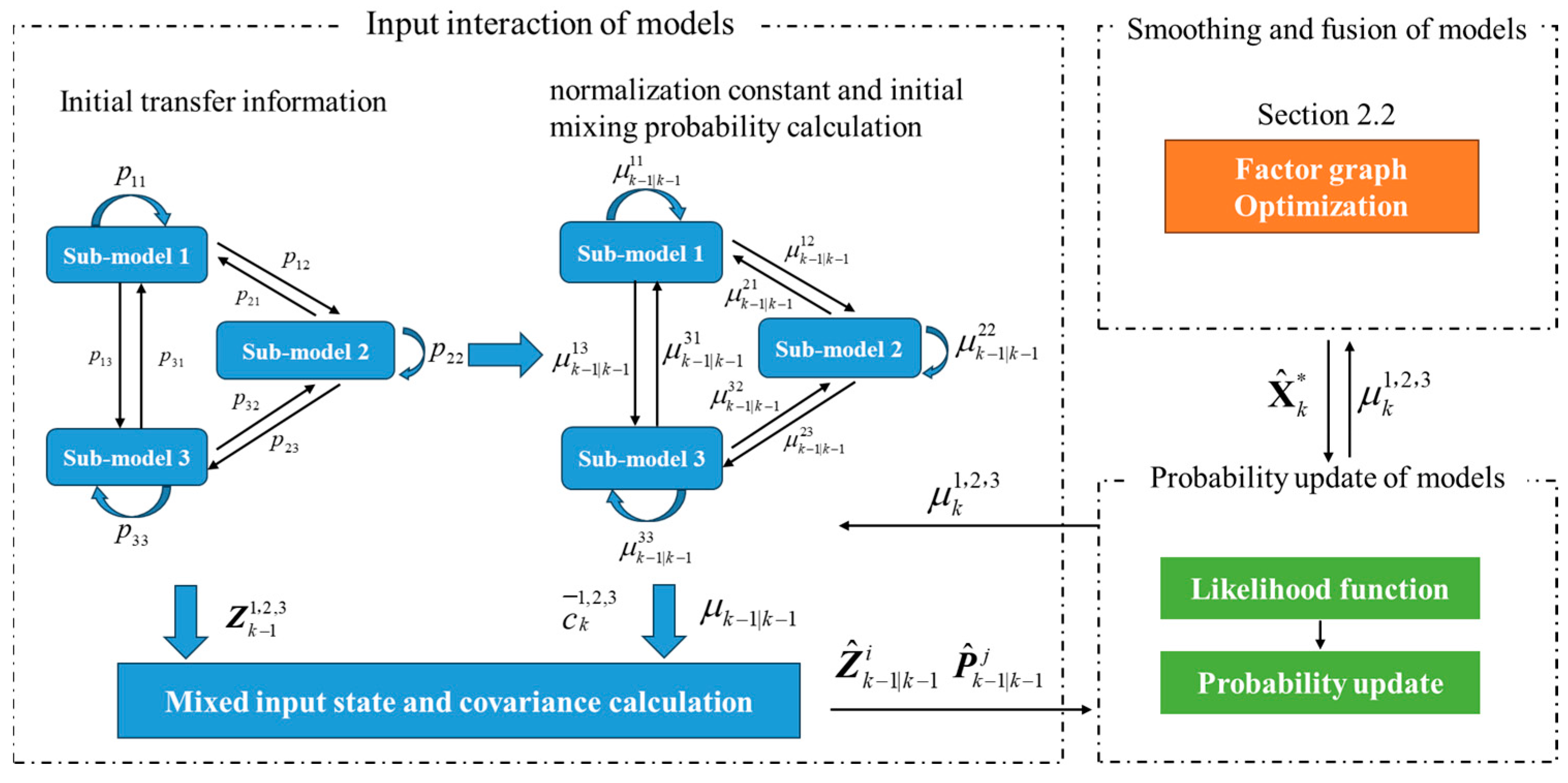
where p k n and v k n represent the position and velocity of the sub-model n at time k , respectively. The information obtained from sub-models is transformed into the world frame. Then, the overall process of the IMMFGO algorithm can be constructed, as in Figure 3.
Figure 3 shows that the IMMFGO algorithm consists of three parts: (1) Input interactions of models, (2) smoothing and fusion of models, and (3) probability update of models. Parts (1) and (2) can provide information for part (3), and the final updated values will optimize the global estimation in part (2) for the next moment. In this paper, only two sub-models are considered, and the function describes the formula of a single sub-model in the case of two sub-models. The number of the sub-models is two; sub-model m 1 is the GNSS navigation system and sub-model m 2 is the LiDAR navigation system. The formula is derived based on two sub-models, and the process of each part is shown as follows.

3.1.1. Input Interactions of Models

Assuming that the process of sub-model m j transforming into sub-model m i follows a Markov chain with a given state transition probability at time k , m i , m j m n , n ( 1 , 2 ) . Then, the transition probability p i j can be defined as follows:
p i j = p { m i ( k ) | m j ( k 1 ) }
Then, calculate the normalization constant c ¯ k j and initial mixing probability μ k 1 | k 1 i j of sub-model m j , which can be expressed as follows:
c ¯ k j = i = 1 n p i j μ k 1 i μ k 1 | k 1 i j = p i j μ k 1 i / c ¯ k j μ k 1 | k 1 j j = p j j μ k 1 i / c ¯ k j
where μ k 1 i represents the model update probability of model m i calculated at time k 1 . μ k 1 | k 1 i j and μ k 1 | k 1 j j represent the initial mixing probability from sub-model m i to m j and m j to itself, respectively. p j j represents the transfer probability to itself of sub-model m j , and is set as one as usual. In the IMMFGO algorithm, the accuracy of the sub-model is evaluated through mixed state inputs. The mixed state variables and covariance of sub-model m j can be defined as follows:
Z ^ k 1 | k 1 0 j = Z k 1 i μ k 1 | k 1 i j + Z k 1 j μ k 1 | k 1 j j P ^ k 1 | k 1 0 j = μ k 1 | k 1 i j { P k 1 i + [ Z k 1 i Z ^ k 1 | k 1 0 j ] [ Z k 1 i Z ^ k 1 | k 1 0 j ] T } +   μ k 1 | k 1 j j { P k 1 j + [ Z k 1 j Z ^ k 1 | k 1 0 j ] [ Z k 1 j Z ^ k 1 | k 1 0 j ] T }
where Z ^ k 1 | k 1 0 j and P ^ k 1 | k 1 0 j represent the mixed state variables and mixed covariance to evaluate the positioning accuracy of the sub-model. Z k 1 i and Z k 1 j represent the measurement information of sub-models m i and m j at time k , respectively. P k 1 i and P k 1 j represent the covariance. The mixed parameters are used to calculate the model update probability relevant to the weights of sub-models during the global optimization process.

3.1.2. Smoothing and Fusion of Models

The factor graph optimization method is employed as the sub-systems information fusion filters, and according to Equation (15), the general function of the IMMFGO in the IMU/GNSS/LiDAR integrated navigation system can be defined as follows:
X ^ k * = arg min X { r p h p ( X k ) p 2 + m [ k N , k ] r i m u ( Z B m + 1 B m , X m ) i m u , m 2 + m [ k N , k ] μ m 1 i r i ( Z m i , X m ) i , m 2 + m [ k N , k ] μ m 1 j r j ( Z m j , X m ) j , m 2 }
where μ m 1 i and μ m 1 j represent the model update probability of model m i and m j at time m 1 , respectively, which are the same as the sensor weights in the navigation system to solve the global optimization at time k . Based on the initial transition probability, the sensor initialization covariance also needs to be optimized to maintain the system initialization accuracy consistent with traditional FGO algorithms; the optimized prior factor can be defined as follows:
f n p r i o r ( X k N ) = 1 2 π μ k N n Σ n p r i o r exp ( ( X k N μ x ) 2 2 μ k N n Σ n p r i o r )
where X k N and μ x represents the system state and mean value at time k N , respectively. Σ n p r i o r represents the covariance of the sub-model n . μ k N n represents the transition probability. When the system framework or sliding window changes, the prior factor will also be optimized accordingly.

3.1.3. Probability Update of Models

The probability update process of the model adopts a likelihood function Λ k j to calculate the update probability μ k j of models. The likelihood function is constructed through a multidimensional Gaussian distribution, which can be defined as follows:
Λ k j = 1 2 π | S k j | exp { 1 2 [ v k j ] [ S k j ] 1 [ v k j ] T }
where v k j and S k j represent the residual of model measurements and the covariance of the model measurements’ residuals, respectively, which can be defined as follows:
v k j = H I M M X ^ k * Z ^ k - 1 | k - 1 0 j S k j = H I M M P k 1 | k 1 0 j [ H I M M ] T + Σ j
where k j represents the covariance of sub-model m j , which is the same as the sensor factor node model. Then, the update probability of model m j can be defined as follows:
c k = j = 1 n Λ k j c ¯ k j μ k j = Λ k j c ¯ k j / c k
When the number of sub-models is one, the update probability is optimized as follows:
μ k j = Λ k j
Compared to AFGO, the proposed IMMFGO algorithm constructs the sub-models based on the precision of sensors and is adaptive to different environments.

3.2. Multi-Stage Fault Detection, Isolation and Recovery Strategy

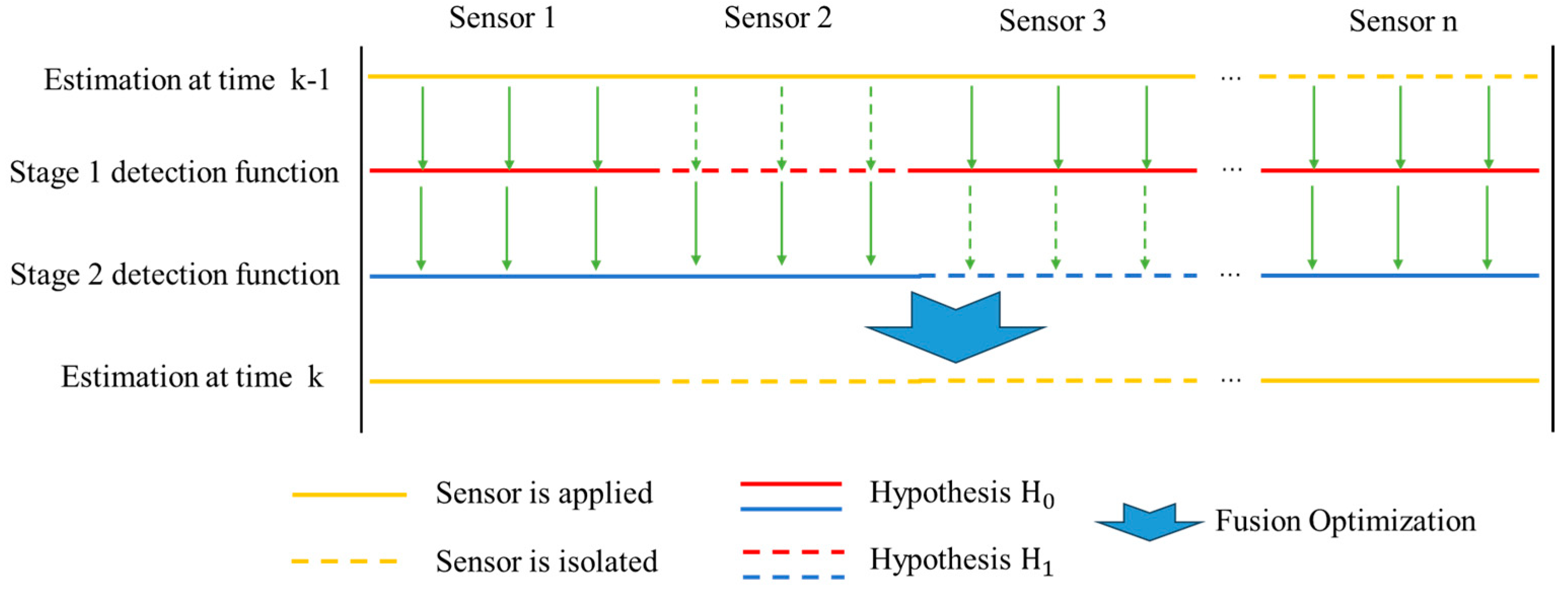
The IMMFGO algorithm can adaptively adjust sensor weights and has specific fault detection capabilities. However, weight adjustment based on factor graph global optimization results makes it difficult to detect the impact of fault information on IMU compensation quickly. Therefore, this part proposes a multi-stage fault detection and isolation method, applying IMMFGO and the Chi-square FDI algorithm [41], which can effectively detect and reflect the impact of faulty sensors on the whole system. The Chi-square FDI algorithm detects faults for auxiliary sensors on the basis of IMU measurements. The overall process of MSFDIR is shown in Figure 4.
Figure 4 shows that the system includes two stages: fault detection based on IMMFGO weight values and Chi-square fault detection based on IMU measurements. For Stage 1, the system detects faults based on the average and minimum weight values. When the average value is less than the threshold T a v e r a g e or the extreme minimum value is less than the threshold T m i n , it is considered that the sensor accuracy is low in a period or there is a sudden interference. The fault detection function is defined as follows:
μ ¯ k n = 1 N * k N k μ k n
When there is no fault, the system is under the no-fault hypothesis H 0 . When the system detects faults, the system is under the fault hypothesis H 1 . Then, the detection function can be expressed as follows:
{ H 0 : n { 1 , 2 , 3 , } , μ ¯ k n < T a v e r a g e & m { k N , k } , μ m n < T m i n H 1   :   n { 1 , 2 , 3 , } ,   μ ¯ k n T a v e r a g e m { k N , k } , μ m n T m i n
When the first stage fault detection function works and the system is under hypothesis H 1 , the accuracy of IMMFGO will decrease and the faulty sensor needs to be isolated. Typically, the FDI algorithm based on IMU measurements is applied to evaluate the performance of assistant sensors [42], and the test statistic function of the residual chi-square value λ k n at time k can be defined as follows:
λ k n = r k n T ( S k n ) 1 r k n
where r k n represents the residual between IMU measurements and assistant sensors. S k n represents the covariance matrix of the residuals. When the function detects no fault, the system is under the no-fault hypothesis H 0 ; otherwise, the system is under hypothesis H 1 . Then, the detection function can be expressed as follows:
{ H 0 : n { 1 , 2 , 3 , } , λ k n < T D n H 1   :   n { 1 , 2 , 3 , } ,   λ k n T D n
where T D n is the second stage detection threshold related to the false alarm probability P f a and standard deviation of sensors. When the system is under hypothesis H 1 , the fault sensors will be isolated and the framework will be reconstructed. When the isolated sensors perform well and the system is under hypothesis H 1 , the isolated sensor will be restored and the framework will be changed. The switching process of the integrated navigation system framework is shown in Figure 5.
Figure 5 shows that the potential fault sensors will be isolated only when both stages are under hypothesis H 1 , and the isolated sensors will be restored only when both stages are under hypothesis H 0 . During the isolation process of the sensors, the IMMFGO algorithm can automatically switch the number of sub-models, while the isolated sensors still work for evaluation and restoration but do not provide navigation information. The recovery judgment of the isolated sensors is dependent on the calculated weights and the system framework and prior information function will also be optimized accordingly. The second stage detection function continuously works in the system. We judge whether the sensor errors have a significant impact on absolute location or IMU results.

4. Experimental Analysis

4.1. Experimental Setup

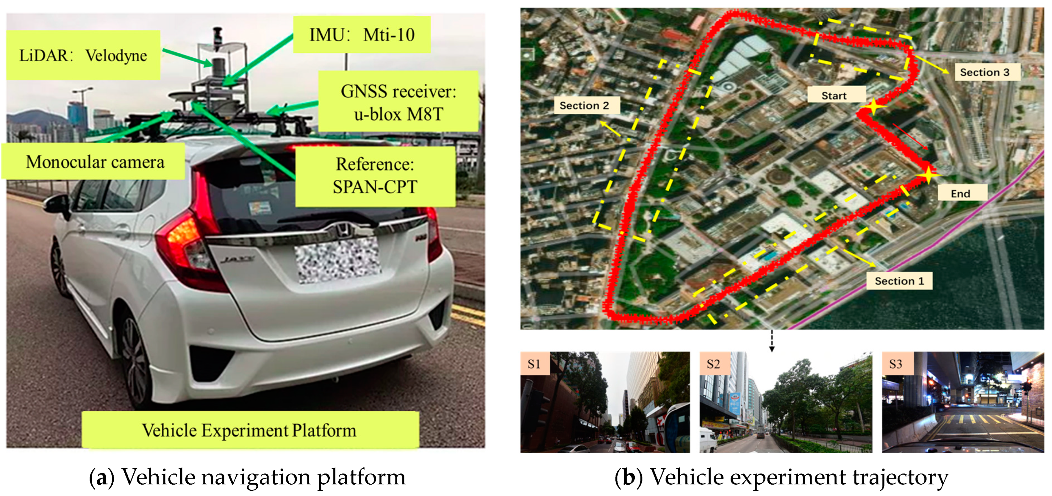
In order to verify the feasibility of the proposed method, actual experiments on vehicle platforms in urban environments were carried out. We use the open-source vehicle city dataset captured by the vehicle platform of the Hong Kong Polytechnic University, China [43]. The vehicle navigation system dataset is suitable for studying the characteristics of sensors and verifying the performance of vehicle navigation systems in urban environments. As shown in Table 1 and Figure 6a, the platform consists of IMU, GNSS, and LiDAR. Furthermore, the ground truth is collected by a high-precision SPAN-CPT system, and the positioning error is up to 2 cm. The extrinsic parameters among sensors were calibrated in advance. The data processing part is under MATLAB platform.
The duration of the experiment is 486 s, with a total length of 2.0 km. In the experiment, there will be multipath interference of GNSS signals and dynamic feature interference from LiDAR. The trajectory and the sections are shown in Figure 6b.
According to environmental characteristics, three typical road sections were selected to validate the proposed algorithm. Road section (1) lasts from 110 s to 160 s, and the vehicle passes through tall buildings while the interference gradually increases. Road section (2) lasts from 250 s to 300 s and the vehicle passes through open areas while the error variation is slight. Road section (3) lasts from 350 s to 450 s, and the vehicle passes through dense areas with sudden interference. The root mean square error (RMSE) is implemented to evaluate the positioning accuracy of different algorithms [44], and we evaluate IMMFGO and MSFDIR based on the typical road sections.

4.2. Experimental Results of IMMFGO

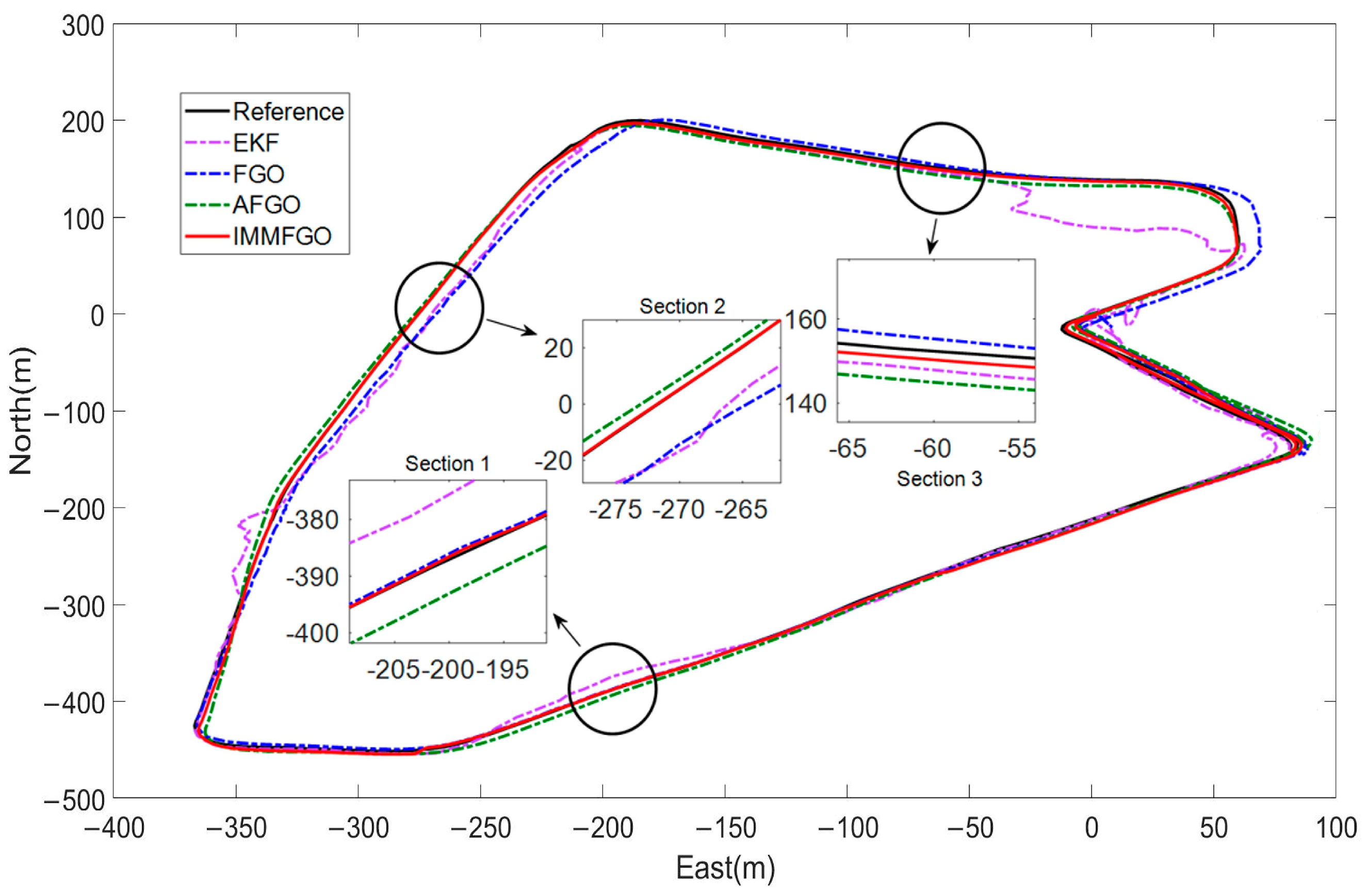
To evaluate the performance of IMMFGO, we compare four algorithms, namely EKF, FGO, AFGO [41], and IMMFGO, and all apply the IMU/GNSS/LiDAR loose-coupled navigation system as the same sensors. During the experiment, the GNSS signal may be interrupted in special road sections, and LiDAR may be affected by the outside environments. Additionally, AFGO and IMMFGO have additional parameters for adaptive optimization. The GNSS threshold is set as 2 m and the LiDAR threshold as 1.5 m for the AFGO algorithm, while the number of sub-models of the IMMFGO algorithm is 2, namely the GNSS navigation sub-model and the LiDAR navigation sub-model. The initial transition probability from GNSS to LiDAR is set as 0.9. The trajectory results of the four algorithms are shown in Figure 7.
As shown in Figure 7, the black solid line represents the reference trajectory. The purple, blue, and green dashed lines represent the trajectory results of EKF, FGO, and AFGO, respectively. The solid red line represents the proposed IMMFGO algorithm. In case of gradually increasing interference in section (1), the positioning results of the proposed IMMFGO algorithm and the traditional FGO algorithm are better. The AFGO algorithm may produce specific errors in the positioning results due to the fixed threshold. In case of stable errors during section (2), the AFGO and IMMFGO algorithms can adaptively adjust sensor weights and achieve good global estimation performance, while the trajectory of the traditional FGO algorithm will be smoothed through global optimization with lower positioning accuracy. In case of sudden interference during section (3), the IMMFGO algorithm can adjust the weights of sensors, thus obtaining better positioning results than the AFGO algorithm, since the threshold set by the AFGO algorithm is unsuitable for unknown sudden faults. Then, east, north, and vertical position errors of different road sections are shown in Figure 8.
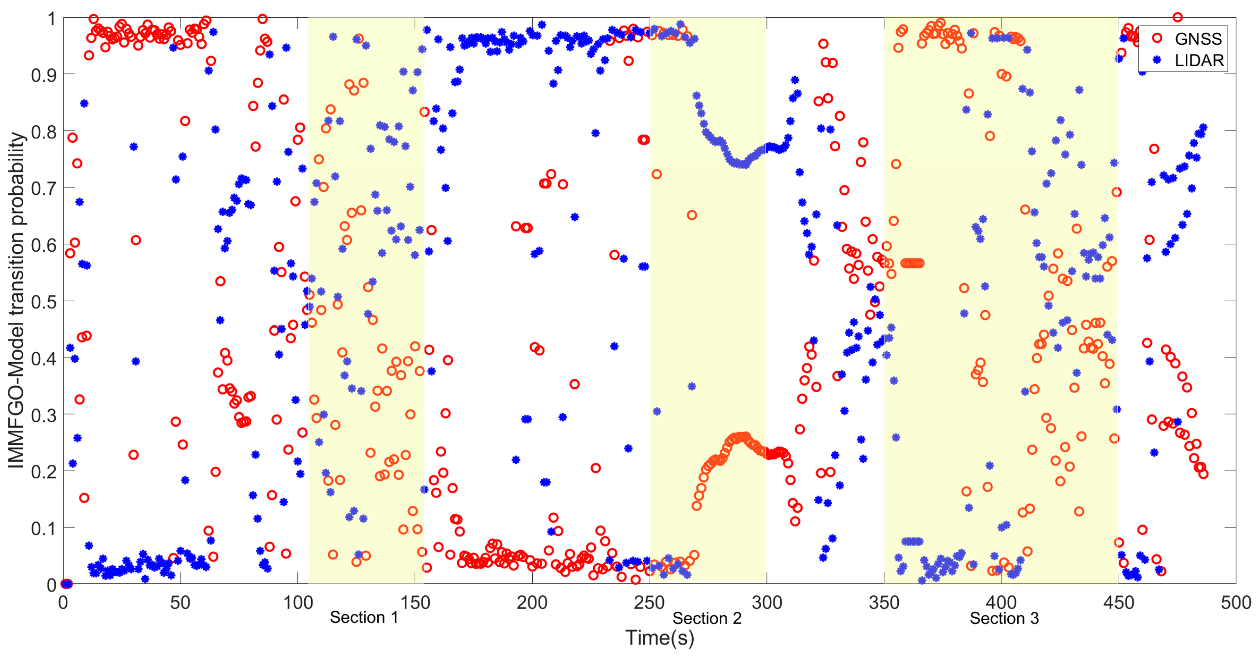
From the trajectory positioning results in Figure 7 and the position errors in Figure 8, it can be seen that both EKF and FGO are strongly affected by external interference, leading to decreased positioning accuracy. However, the trajectory of the FGO algorithm can be optimized through historical information, thereby improving specific performance. Compared to other algorithms, AFGO and IMMFGO have the ability to adaptively optimize the weights in case of interference. While the AFGO algorithm is based on a fixed detection threshold according to personal experience, and its performance is poor in dynamic or sudden interference situations, the proposed IMMFGO algorithm changes sensor weights based on sensor performance and environmental changes, of which the threshold is adaptively adjusted, resulting in good performance under different interference conditions. The probability transition results of the IMMFGO algorithm are shown in Figure 9.
Figure 9 shows the transition probability of the IMMFGO sub-models. IMMFGO can reduce the impact of environmental interference on positioning accuracy by switching model probabilities, which has good results in global positioning. According to the changes in transition probability for different road sections, it is clear that when sensor accuracy decreases, the corresponding model probabilities also decrease, reducing the impact of interference on positioning results and improving positioning accuracy. To quantitatively evaluate the performance of our algorithm, we calculated the RMSE of each method. Table 2 shows the quantitative results of four algorithms.
Table 2 shows that the 3D RMSE of EKF in global accuracy is 14.14 m. At the same time, FGO, optimized by combining historical measurement information, has a 3D RMSE of 10.18 m, which improved by 28% compared to EKF. AFGO and IMMFGO, with a weight adjustment trajectory based on FGO, have achieved certain improvements in positioning accuracy. The 3D RMSE of AFGO is 6.4 m, which improved by 37.1% compared to FGO. The 3D RMSE of IMMFGO is 4.88 m, which improved by 23.7% compared to AFGO, and the positioning results in the east, north and vertical directions have better performances. The experiment shows that compared to the AFGO algorithm, which can adjust weights through preset thresholds, IMMFGO has better performance in complex urban environments. On the basis of the traditional FGO algorithm, IMMFGO can better achieve precise positioning results for vehicles. The proposed system is based on the sensor with the lowest frequency for information fusion. In this experiment, the signal output frequency is 1 Hz, which can meet the positioning and robustness requirements of actual vehicle navigation systems. The comparison results with existing algorithms are shown in Table 3.
Table 3 shows the performance of proposed algorithm and the previous IMU/GNSS/LiDAR integrated navigation algorithm [43]. In complex urban environments, GNSS or LiDAR alone for navigation tends to have poor performance. IMMFGO achieves better performance than traditional LIO-SAM algorithm because of poor GNSS performance and similar performance of optimal adaptive Integrated GNSS-RTK/LIO algorithm in complex urban canyons. Contrary to adaptive integrated GNSS-RTK/LIO which can only have good performance by testing different thresholds, IMMFGO algorithm evaluates the models based on the output of sub-models which does not rely on auxiliary information and has better environmental adaptability.

4.3. Experimental Results of MSFDIR

In Part 4.2, we analyzed and validated the performance of the IMMFGO algorithm through vehicle experiments. Based on the work above, we will further analyze the impact of fault detection, isolation, and recovery functions.
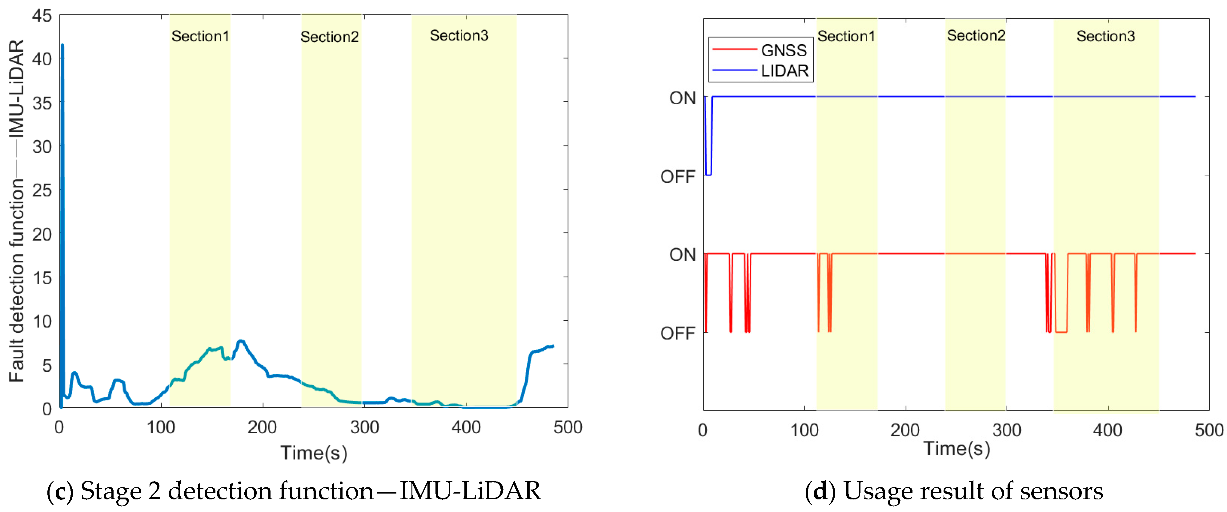
Based on the MSFDIR algorithm proposed in Part 3.2, the first stage average and minimum fault detection threshold based on IMMFGO is set to 0.05 and 0.02, and the stage 2 fault detection threshold is set as five times the standard deviation of sensors. The recovery threshold is set as the same. Figure 10 shows the results of the fault detection functions and the usage of sensors.
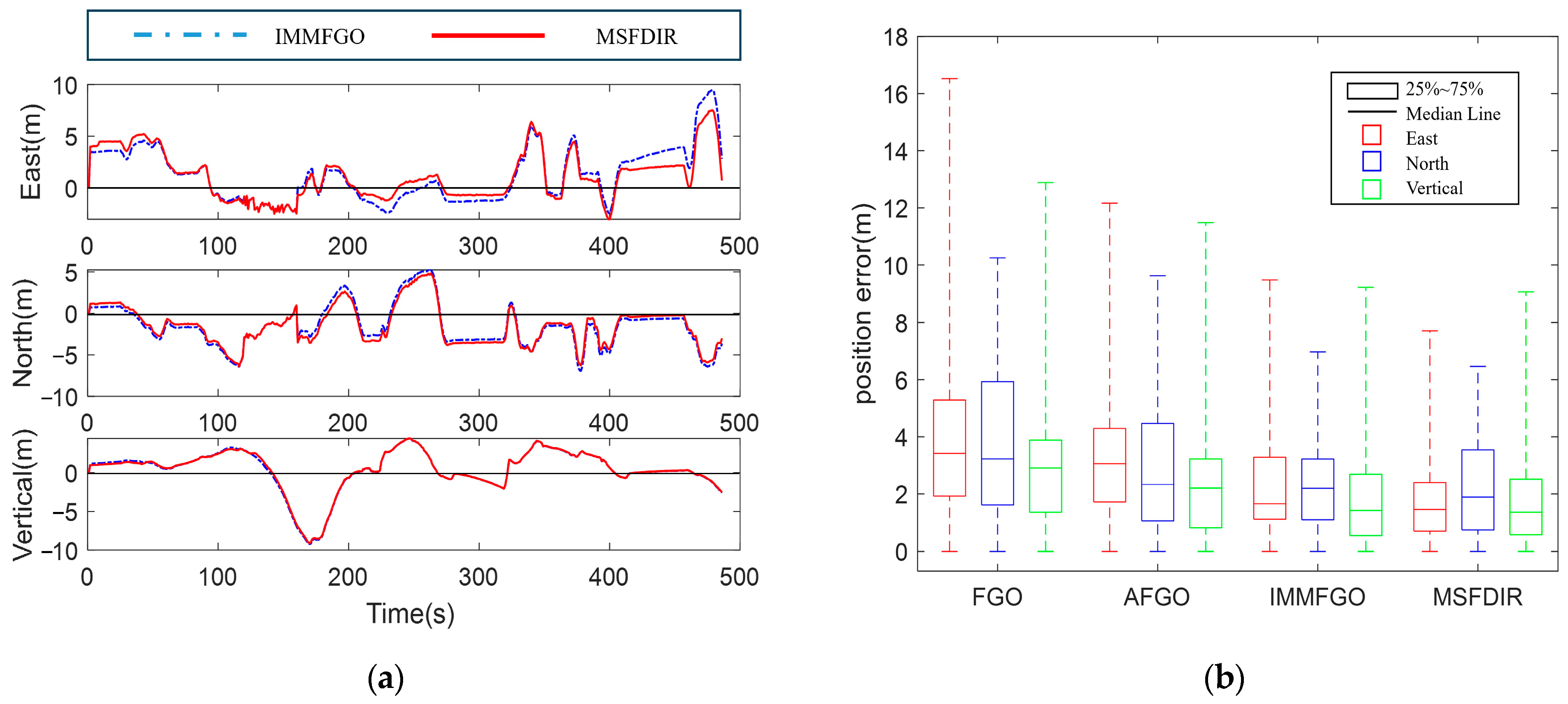
From Figure 10, we can see that in road section (1), when there is a slowly changing error, the stage 1 detection function can respond to the error, and the stage 2 detection function can detect errors that have a significant impact on the IMU and isolate the sensor. In road section (2), when there is a stable error, the IMMFGO algorithm can automatically optimize sensor weights, thus avoiding significant errors. In road section (3), when there are step faults, the stage 1 and stage 2 detection functions can identify errors that significantly impact position accuracy and isolate the corresponding sensors. In other road sections, gradual and step faults that have a significant impact on system performance can also be detected and isolated to ensure the performance of the IMMFGO algorithm and improve system accuracy. The position error results for the east, north, and vertical directions of the proposed IMMFGO and MSFDIR algorithm are shown in Figure 11a. The box diagram of position errors also shows the superiority of the proposed method in Figure 11b.
Figure 11a shows that when a significant fault occurs, the factor graph optimization algorithm has the characteristic of global optimization based on historical information, which will generate cumulative errors. The MSFDIR algorithm can detect and reduce the impact of significant or slowly changing faults, thus improving the performance of system state estimation based on the IMMFGO algorithm. The RMSE of several factor graph optimization algorithms for quantitative analysis is shown in Table 4.
Figure 11b and Table 4 show that after adopting the MSFDIR function, the positioning accuracy is improved and the 3D position error is decreased to 4.42 m. Compared to the IMMFGO algorithm, the accuracy has improved by 9.4%, and the positioning accuracy in the east, north, and vertical directions has improved. The proposed MSFDIR function can obtain the usage information of sensors to provide more information for vehicle navigation systems to ensure system security. The MSFDIR function can compensate for the problem of slowly increasing or significant faults leading to a decrease in the positioning accuracy of the IMMFGO algorithm. Meanwhile, MSFDIR also provides a reference for fault warnings in vehicle navigation systems. At the same time, the real-time performance of MSFDIR can also meet the actual needs of vehicle navigation systems.

5. Discussion

In this paper, a multi-source integrated navigation system based on factor graph optimization is proposed. Aiming to reduce the impact of interfered sensors under a challenging urban environment, the interactive multiple models algorithm based on factor graph optimization is applied, and the multi-stage fault detection, isolation, and recovery function provides flexible navigation frameworks for different conditions. The vehicle experiment shows that the proposed approach has a good navigation performance in urban environments, and the system can effectively identify and isolate faulty sensors. The proposed IMMFGO and MSFDIR algorithms provide a new idea for multi-source information fusion, but there still exists some shortcomings for further exploration, summarized as follows:
  • The IMMFGO algorithm can be applied to the navigation system in the case of multiple sub-models. We only verify the performance of the algorithm for two sub-models, and more situations need to be considered later;
  • The MSFDIR algorithm provides a feasible solution for the detection, isolation, and recovery of faulty sensors, and the performance of other solutions should be studied on this basis;
  • We select a representative urban environment experiment to validate the proposed method. It is fascinating to explore more urban data and experiments to verify the universality of the proposed scheme.

6. Conclusions

Aiming at the demand for high-precision vehicle positioning in complex urban environments, an IMU/GNSS/LiDAR loosely coupled navigation system is constructed based on the studied factor graph optimization algorithm. Then, IMMFGO, an adaptive optimization algorithm, is applied to evaluate the performance of multiple sensors and to automatically adjust sensor weights for better global estimation. On this basis, the proposed MSFDIR scheme provides a feasible solution for framework optimization, which is capable of detecting, isolating, and restoring target sensors and automatically adjusting the system framework. Furthermore, the superiority of the proposed method compared with traditional methods has been verified through vehicle experiments in typical urban canyons. The results indicate that the proposed IMMFGO outperforms AFGO in accuracy, and the MSFDIR scheme can optimize the navigation framework while improving positioning accuracy to a certain extent.

Author Contributions

Conceptualization, Q.Z.; Data curation, C.S.; Formal analysis, F.L.; Investigation, C.S.; Methodology, S.W.; Project administration, Q.Z.; Software, S.W.; Supervision, F.L. and J.L.; Writing—original draft, S.W.; Writing—review and editing, S.W. All authors have read and agreed to the published version of the manuscript.

Funding

This work is funded by the National Natural Science Foundation of China (NO. 61533008, 61603181, 61673208, 61873125).

Data Availability Statement

The data that support the findings of this study are available from the corresponding author upon reasonable request.

Acknowledgments

The dataset was supported by Hong Kong Polytechnic University, which is deeply appreciated.

Conflicts of Interest

The authors declare no conflicts of interest.

References

  1. Chang, D.; Johnson-Roberson, M.; Sun, J. An Active Perception Framework for Autonomous Underwater Vehicle Navigation Under Sensor Constraints. IEEE Trans. Control Syst. Technol. 2022, 30, 2301–2316. [Google Scholar] [CrossRef]
  2. Liu, M.; Zhao, F.; Niu, J.W.; Liu, Y. ReinforcementDriving: Exploring Trajectories and Navigation for Autonomous Vehicles. IEEE Trans. Intell. Transp. Syst. 2021, 22, 808–820. [Google Scholar] [CrossRef]
  3. Zhang, R.B.; Wu, Y.Z.; Zhang, L.X.; Xu, C.; Gao, F. Autonomous and Adaptive Navigation for Terrestrial-Aerial Bimodal Vehicles. IEEE Rob. Autom. Lett. 2022, 7, 3008–3015. [Google Scholar] [CrossRef]
  4. Sun, K.; Zeng, Q.; Liu, J.; Qiu, W.; Shi, J. Modified attitude factor graph fusion method for unmanned helicopter under atmospheric disturbance. Chin. J. Aeronaut. 2022, 35, 285–297. [Google Scholar] [CrossRef]
  5. Jiang, H.T.; Li, T.; Song, D.; Shi, C. An Effective Integrity Monitoring Scheme for GNSS/INS/Vision Integration Based on Error State EKF Model. IEEE Sens. J. 2022, 22, 7063–7073. [Google Scholar] [CrossRef]
  6. Qin, H.M.; Wang, X.; Wang, G.C.; Hu, M.J.; Bian, Y.G.; Qin, X.H.; Ding, R.J. A novel INS/USBL/DVL integrated navigation scheme against complex underwater environment. Ocean Eng. 2023, 286. [Google Scholar] [CrossRef]
  7. Taghizadeh, S.; Safabakhsh, R. An Integrated INS/GNSS System With an Attention-Based Deep Network for Drones in GNSS Denied Environments. IEEE Aerosp. Electron. Syst. Mag. 2023, 38, 14–25. [Google Scholar] [CrossRef]
  8. Taghizadeh, S.; Safabakhsh, R. An integrated INS/GNSS system with an attention-based hierarchical LSTM during GNSS outage. GPS Solutions 2023, 27, 71. [Google Scholar] [CrossRef]
  9. Zhang, J.C.; Wen, W.S.; Huang, F.; Chen, X.D.; Hsu, L.T. Coarse-to-Fine Loosely-Coupled LiDAR-Inertial Odometry for Urban Positioning and Mapping. Remote Sens. 2021, 13, 2371. [Google Scholar] [CrossRef]
  10. Sun, K.C.; Zeng, Q.H.; Liu, J.Y.; Wang, S.Y. Fault Detection of Resilient Navigation System Based on GNSS Pseudo-Range Measurement. Appl. Sci. 2022, 12, 5313. [Google Scholar] [CrossRef]
  11. Ambroziak, L.; Ciezkowski, M.; Wolniakowski, A.; Romaniuk, S.; Bozko, A.; Oldziej, D.; Kownacki, C. Experimental tests of hybrid VTOL unmanned aerial vehicle designed for surveillance missions and operations in maritime conditions from ship-based helipads. J. Field Rob. 2022, 39, 203–217. [Google Scholar] [CrossRef]
  12. Shen, C.; Xiong, Y.F.; Zhao, D.H.; Wang, C.G.; Cao, H.L.; Song, X.; Tang, J.; Liu, J. Multi-rate strong tracking square-root cubature Kalman filter for MEMS-INS/GPS/polarization compass integrated navigation system. Mech. Syst. Sig. Process. 2022, 163, 108146. [Google Scholar] [CrossRef]
  13. Shen, C.; Zhang, Y.; Tang, J.; Cao, H.L.; Liu, J. Dual-optimization for a MEMS-INS/GPS system during GPS outages based on the cubature Kalman filter and neural networks. Mech. Syst. Sig. Process. 2019, 133, 106222. [Google Scholar] [CrossRef]
  14. Ma, X.; Liu, X.; Zhang, T.; Liu, X.; Xu, G. AUV multi-sensor integrated navigation algorithm based on factor graph. J. Chin. Inert. Technol. 2019, 27, 454–459. [Google Scholar]
  15. Indelman, V.; Williams, S.; Kaess, M.; Dellaert, F. Information fusion in navigation systems via factor graph based incremental smoothing. Rob. Auton. Syst. 2013, 61, 721–738. [Google Scholar] [CrossRef]
  16. Xu, J.; Yang, G.L.; Sun, Y.D.; Picek, S. A Multi-Sensor Information Fusion Method Based on Factor Graph for Integrated Navigation System. IEEE Access 2021, 9, 12044–12054. [Google Scholar] [CrossRef]
  17. Vallve, J.; Sola, J.; Andrade-Cetto, J. Pose-graph SLAM sparsification using factor descent. Rob. Auton. Syst. 2019, 119, 108–118. [Google Scholar] [CrossRef]
  18. Tu, M.Y.; Zeng, P.L.; Wu, Q.X.; Jing, T.; Tian, Y.Y.; Luo, Y.B.; Mao, W.D. Lidar SLAM Based on Particle Filter and Graph Optimization for Substation Inspection. IEEE Access 2022, 10, 127540–127549. [Google Scholar] [CrossRef]
  19. Lu, D.F.; Zhang, Y.W.; Gong, Z.W.; Wu, T.N. A SLAM Method Based on Multi-Robot Cooperation for Pipeline Environments Underground. Sustainability 2022, 14, 12995. [Google Scholar] [CrossRef]
  20. Chen, H.L.; Wu, W.; Zhang, S.; Wu, C.H.; Zhong, R.F. A GNSS/LiDAR/IMU Pose Estimation System Based on Collaborative Fusion of Factor Map and Filtering. Remote Sens. 2023, 15, 790. [Google Scholar] [CrossRef]
  21. Bouchareb, I.; Bentounsi, A.; Lebaroud, A. Fault detection and diagnosis in a set “inverter-switched reluctance motor” based on pattern recognition using Kalman filter prediction. Int. J. Appl. Electromagn. Mech. 2014, 45, 495–502. [Google Scholar] [CrossRef]
  22. Zabalegui, P.; De Miguel, G.; Goya, J.; Moya, I.; Mendizabal, J.; Adín, I. Residual based fault detection and exclusion methods applied to Ultra-Wideband navigation. Measurement 2021, 179, 109350. [Google Scholar] [CrossRef]
  23. Jurado, J.; Raquet, J.; Kabban, C.M.S. Single-Filter Finite Fault Detection and Exclusion Methodology for Real-Time Validation of Plug-and-Play Sensors. IEEE Trans. Aerosp. Electron. Syst. 2021, 57, 66–75. [Google Scholar] [CrossRef]
  24. Elsayed, H.; El-Mowafy, A.; Wang, K. A new method for fault identification in real-time integrity monitoring of autonomous vehicles positioning using PPP-RTK. GPS Solut. 2024, 28, 32. [Google Scholar] [CrossRef]
  25. Wang, Z.P.; Li, B.; Dan, Z.Q.; Wang, H.X.; Fang, K. 3D LiDAR Aided GNSS/INS Integration Fault Detection, Localization and Integrity Assessment in Urban Canyons. Remote Sens. 2022, 14, 4641. [Google Scholar] [CrossRef]
  26. Gao, Y.T.; Gao, Y.; Liu, B.Y.; Jiang, Y. Enhanced fault detection and exclusion based on Kalman filter with colored measurement noise and application to RTK. GPS Solut. 2021, 25, 82. [Google Scholar] [CrossRef]
  27. Kheirandish, M.; Yazdi, E.A.; Mohammadi, H.; Mohammadi, M. A fault-tolerant sensor fusion in mobile robots using multiple model Kalman filters. Rob. Auton. Syst. 2023, 161, 104343. [Google Scholar] [CrossRef]
  28. Xiong, J.; Xiong, Z.; Zhuang, Y.; Cheong, J.W.; Dempster, A.G. Fault-Tolerant Cooperative Positioning Based on Hybrid Robust Gaussian Belief Propagation. IEEE Trans. Intell. Transp. Syst. 2023, 24, 6425–6431. [Google Scholar] [CrossRef]
  29. Wang, L.; Li, S.X. Enhanced Multi-sensor Data Fusion Methodology based on Multiple Model Estimation for Integrated Navigation System. Int. J. Control Autom. 2018, 16, 295–305. [Google Scholar] [CrossRef]
  30. Thanaraj, T.; Low, K.H.; Ng, B.F. Actuator fault detection and isolation on multi-rotor UAV using extreme learning neuro-fuzzy systems. ISA Trans. 2023, 138, 168–185. [Google Scholar] [CrossRef] [PubMed]
  31. Forkuo, G.O.; Borz, S.A. Accuracy and inter-cloud precision of low-cost mobile LiDAR technology in estimating soil disturbance in forest operations. Front. For. Glob. Chang. 2023, 6, 1224575. [Google Scholar] [CrossRef]
  32. Shen, Z.H.; Wang, J.B.; Pang, C.L.; Lan, Z.Y.; Fang, Z. A LiDAR-IMU-GNSS fused mapping method for large-scale and high-speed scenarios. Measurement 2024, 225, 113961. [Google Scholar] [CrossRef]
  33. Zhang, H.M.; Xia, X.; Nitsch, M.M.; Abel, D. Continuous-Time Factor Graph Optimization for Trajectory Smoothness of GNSS/INS Navigation in Temporarily GNSS-Denied Environments. IEEE Rob. Autom. Lett. 2022, 7, 9115–9122. [Google Scholar] [CrossRef]
  34. Jiang, C.H.; Chen, Y.W.; Xu, B.; Jia, J.X.; Sun, H.B.; Chen, C.; Duan, Z.Y.; Bo, Y.M.; Hyyppä, J. Vector Tracking Based on Factor Graph Optimization for GNSS NLOS Bias Estimation and Correction. IEEE Internet Things J. 2022, 9, 16209–16221. [Google Scholar] [CrossRef]
  35. Li, Q.M.; Zhang, L.W.; Wang, X.L. Loosely Coupled GNSS/INS Integration Based on Factor Graph and Aided by ARIMA Model. IEEE Sens. J. 2021, 21, 24379–24387. [Google Scholar] [CrossRef]
  36. Yin, F.; Butts, C.T. Highly scalable maximum likelihood and conjugate Bayesian inference for ERGMs on graph sets with equivalent vertices. PLoS ONE 2022, 17, e0273039. [Google Scholar] [CrossRef]
  37. Bai, S.Y.; Lai, J.Z.; Lyu, P.; Cen, Y.T.; Ji, B.W. Improved Preintegration Method for GNSS/IMU/In-Vehicle Sensors Navigation Using Graph Optimization. IEEE Trans. Veh. Technol. 2021, 70, 11446–11457. [Google Scholar] [CrossRef]
  38. Laconte, J.; Lisus, D.; Barfoot, T.D. Toward Certifying Maps for Safe Registration-Based Localization Under Adverse Conditions. IEEE Rob. Autom. Lett. 2024, 9, 1572–1579. [Google Scholar] [CrossRef]
  39. Yuan, R.H.; Taylor, C.N.; Nykl, S.L.; Taylor, C. Accurate Covariance Estimation for Pose Data From Iterative Closest Point Algorithm. Navig. J. Inst. Navig. 2023, 70, navi.562. [Google Scholar] [CrossRef]
  40. Wang, Y.; Gong, Y.X.; Yang, H.K. A mobile localization algorithm based on fuzzy estimation for serious NLOS scenes. Peer--Peer Netw. Appl. 2023, 16, 2271–2289. [Google Scholar] [CrossRef]
  41. Wei, X.K.; Li, J.; Zhang, D.B.; Feng, K.Q. An improved integrated navigation method with enhanced robustness based on factor graph. Mech. Syst. Sig. Process. 2021, 155, 107565. [Google Scholar] [CrossRef]
  42. Zhu, Y.X.; Wu, X.X. A Fault-Tolerant Scheme Based on MSVR for Integrated Navigation. IEEE Sens. J. 2022, 22, 18740–18750. [Google Scholar] [CrossRef]
  43. Zhang, J.C.; Wen, W.S.; Huang, F.; Wang, Y.L.; Chen, X.D.; Hsu, L.T. GNSS-RTK Adaptively Integrated with LiDAR/IMU Odometry for Continuously Global Positioning in Urban Canyons. Appl. Sci. 2022, 12, 5193. [Google Scholar] [CrossRef]
  44. Hashemi, M.; Shami, E. New fault detection and fault-tolerant scheme for Doppler velocity logger outage in ocean navigation systems. J. Navig. 2021, 74, 409–424. [Google Scholar] [CrossRef]
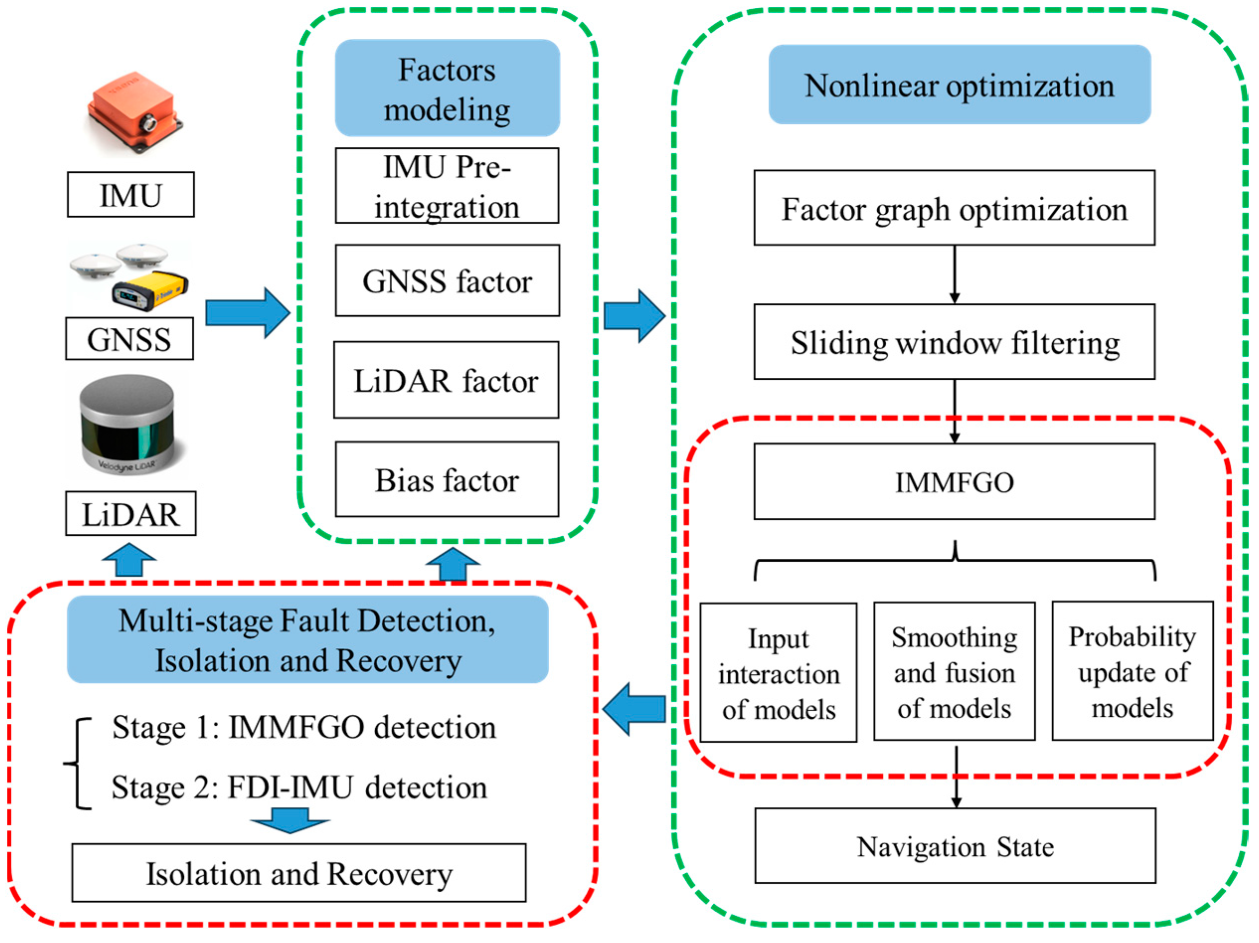
Figure 1. Overview of the proposed method.
Remotesensing 16 01651 g001
Figure 2. Schematic diagram of factor graph optimization by the proposed IMU/GNSS/LiDAR integrated navigation system.
Remotesensing 16 01651 g002
Figure 3. Schematic diagram of the proposed IMMFGO algorithm. The figure shows the process of the IMMFGO algorithm when n = 3.
Remotesensing 16 01651 g003
Figure 4. Schematic diagram of the proposed MSFDIR algorithm. There are three auxiliary sensors, and the isolation and recovery functions are shown when a single sensor is faulty.
Remotesensing 16 01651 g004
Figure 5. Schematic diagram of sensor isolation and recovery.
Remotesensing 16 01651 g005
Figure 6. The platform and trajectory of vehicle experiment collected in the urban canyon. (a) The vehicle navigation platform and distribution of sensors; (b) the trajectory of the vehicle experiment and division of different road sections based on environmental characteristics.
Remotesensing 16 01651 g006
Figure 7. Trajectory diagram of four algorithms and three sections (unit: meters).
Remotesensing 16 01651 g007
Figure 8. Schematic diagram of position error results of four algorithms. (ac) are east, north, and vertical position error results, respectively.
Remotesensing 16 01651 g008
Figure 9. Results of the IMMFGO model transition possibility.
Remotesensing 16 01651 g009
Figure 10. Results of MSFDIR in vehicle experiments. (a) is the result of the stage 1 IMMFGO fault detection function. (b,c) are the results of the stage 2 GNSS and LiDAR fault detection function based on IMU, respectively. (d) is the usage result of GNSS and LiDAR.
Remotesensing 16 01651 g010aRemotesensing 16 01651 g010b
Figure 11. (a) Comparison results of the position errors in the east, north, and vertical directions between the proposed IMMFGO and MSFDIR. (b) The box diagram of position errors.
Remotesensing 16 01651 g011
Table 1. Vehicle navigation platforms and sensors information.
SourcesParameter TypesParameter Values
Xsens-Mti-10 IMUFrequency100 Hz
Gyroscope random drift error18 °/h
Accelerometer random drift error15 μg
U-blox M8T
GNSS receiver
Frequency1 Hz
Positioning accuracy2.5 m
HDL-32E Velodyne LiDARFrequency10 Hz
Measurement Range80 m
Range Accuracy2 cm
Table 2. RMSE of the four algorithms and the improvement of IMMFGO to AGO (unit: meters).
Types of ErrorEKFFGOAFGOIMMFGOImprovement
East8.078.163.662.8522.1%
North10.053.963.952.9026.5%
Vertical5.874.623.462.7221.3%
3D14.1410.186.44.8823.7%
Table 3. 3D RMSE of proposed algorithm and previous works.
Methods3D RMSE (m)
Alone GNSS42.02
LIO-SAM19.89
Adaptive Integrated GNSS-RTK/LIO
( e l t h = 90°, 35°, 15°)
25.33, 18.88, 4.12
IMMFGO4.88
Table 4. RMSE of five algorithms and the improvement from MSFDIR to IMMFGO (unit: meters).
Types of ErrorEKFFGOAFGOIMMFGOMSFDIRImprovement
East9.078.163.662.852.647.4%
North10.053.963.952.902.668.3%
Vertical5.874.623.462.722.3513.6%
3D14.1410.186.44.884.429.4%
Disclaimer/Publisher’s Note: The statements, opinions and data contained in all publications are solely those of the individual author(s) and contributor(s) and not of MDPI and/or the editor(s). MDPI and/or the editor(s) disclaim responsibility for any injury to people or property resulting from any ideas, methods, instructions or products referred to in the content.