Abstract
The semantic segmentation of drone LiDAR data is important in intelligent industrial operation and maintenance. However, current methods are not effective in directly processing airborne true-color point clouds that contain geometric and color noise. To overcome this challenge, we propose a novel hybrid learning framework, named SSGAM-Net, which combines supervised and semi-supervised modules for segmenting objects from airborne noisy point clouds. To the best of our knowledge, we are the first to build a true-color industrial point cloud dataset, which is obtained by drones and covers 90,000 m2. Secondly, we propose a plug-and-play module, named the Global Adjacency Matrix (GAM), which utilizes only few labeled data to generate the pseudo-labels and guide the network to learn spatial relationships between objects in semi-supervised settings. Finally, we build our point cloud semantic segmentation network, SSGAM-Net, which combines a semi-supervised GAM module and a supervised Encoder–Decoder module. To evaluate the performance of our proposed method, we conduct experiments to compare our SSGAM-Net with existing advanced methods on our expert-labeled dataset. The experimental results show that our SSGAM-Net outperforms the current advanced methods, reaching in mIoU, which ranges from to higher than other methods, achieving a competitive level.
1. Introduction
Semantic segmentation of airborne LiDAR point clouds plays a critical role in intelligent industrial operation and maintenance (O&M). It automatically detects and classifies equipment in industrial scenarios, helping to improve production efficiency and reduce downtime [1,2]. For example, the semantic segmentation of airborne electrical substation point clouds simplifies industrial defect detection and facilitates the development of digital twins in the power sectors [3,4,5,6]. With the development of remote sensing technology, using drones equipped with RGB cameras and LiDAR sensors to acquire remote sensing images and airborne LiDAR point clouds offers an efficient way to acquire comprehensive scene information [7,8], providing basic data for intelligent industrial O&M and applications of building information modeling (BIM) model in various fields, such as cultural heritage protection [9], smart cities [10,11], and energy [12].
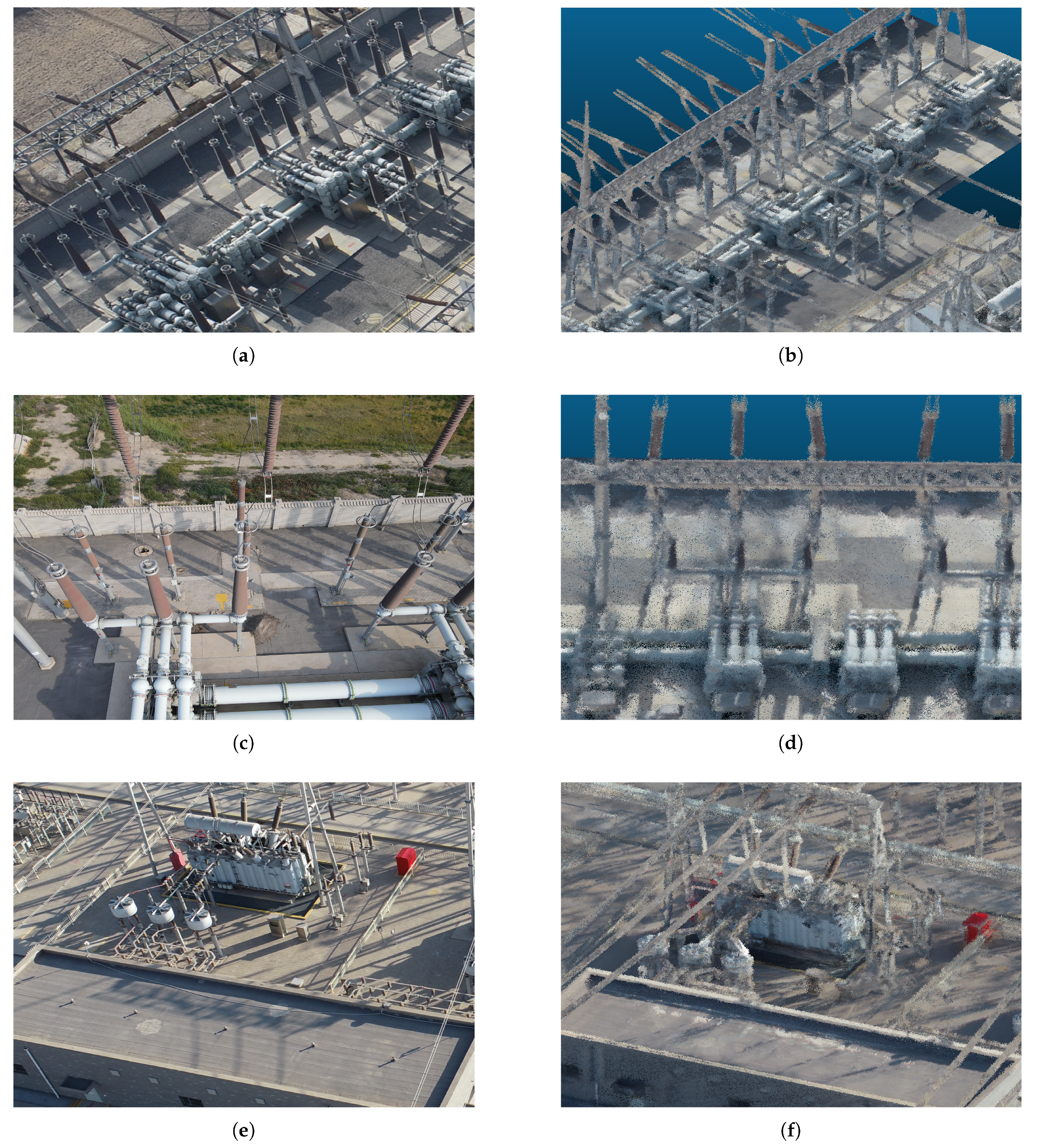
With the development of 3D model reconstruction, it is possible to utilize drone remote sensing images and airborne LiDAR point clouds to reconstruct true-color point clouds via commercial softwares [13]. Compared with RGB images or LiDAR point clouds, the fused true-color point clouds exhibit significant advantages. Primarily, true-color point clouds provide an exhaustive description of the object geometry, capturing details often lost in two-dimensional representations [14]. Furthermore, they provide color details in addition to 3D geometry. However, the imprecision of laser range measurements and the movement of the aircraft introduce uncertainties and errors in the 3D coordinates of each point, so the resulting true-color point clouds contain substantial geometric noise [15]. Additionally, the registration errors of RGB images during the reconstruction cause color information shifts of the true-color point clouds, drastically degrading the quality of the airborne true-color point clouds [13], as shown in Figure 1b,d,f,h.
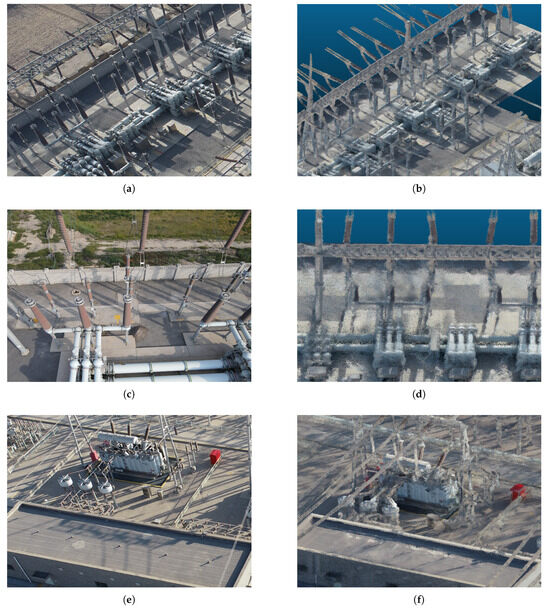

Figure 1.
Images of the electrical substations (a,c,e,g) and the corresponding airborne true-color point clouds (b,d,f,h).
Therefore, noisy true-color point clouds present significant challenges for the semantic segmentation of such point clouds. The inherent noise in such point clouds impairs the efficacy of traditional algorithms, such as principal component analysis (PCA) and support vector machines (SVM), in accurately capturing the geometric structure of the objects [5,16]. Recent advances in deep learning (DL) have facilitated the development of sophisticated algorithms for point cloud semantic segmentation, leading to significant breakthroughs in different domains such as industrial O&M [17,18], autonomous driving [19,20], and smart cities [21,22]. The DL-based semantic segmentation methods for point clouds can be roughly divided into four categories: projection-based [23,24,25,26,27], voxel-based [28,29,30,31], point-wise multilayer perceptron (MLP) [32,33,34,35,36], and point convolution methods [37,38,39,40]. All of these methods perform 3D semantic learning in supervised settings, relying on the geometric structure and color information within the point clouds. Therefore, when both pieces of information are severely distorted (e.g., noisy true-color point clouds), as depicted in Figure 1, these methods become ineffective.
Based on the aforementioned four categories of methods, various researchers have engaged in research concerning the semantic segmentation of drone LiDAR data in recent years. Zeng et al. [41] introduced RRDAN for the semantic segmentation of airborne LiDAR point clouds. They refined KPConv [40] by integrating attention mechanisms and recurrent residual learning. The effectiveness of RRDAN was validated on an artificially noisy airborne point cloud dataset without color information. In addition, a more previous approach, called LGENet [42], was proposed for the semantic segmentation of airborne LiDAR point clouds. It fused a combination of KPConv and SegECC blocks, enhanced with a spatial-channel attention mechanism. LGENet’s effectiveness was also demonstrated in a synthetic noisy airborne point cloud dataset that lacked color information. Therefore, we chose RRDAN, a more up-to-date method, for the comparative experiments. It should be noted that both researchers artificially added noise into the airborne point cloud to test the robustness of their methods in noisy point clouds. However, the added noise is not able to fit the actual noise distribution caused by aircraft movement, imprecise laser range measurements, and point cloud fusion during post-processing. As a result, significant challenges are posed by adopting these methods on airborne noisy true-color point clouds acquired by drones.
The objective of this study is to develop a hybrid learning-based semantic segmentation network capable of accurately segmenting industrial objects from airborne noisy true-color point clouds. In this study, we propose a plug-and-play module, named the Global Adjacency Matrix (GAM), to guide the network to learn global contextual relationships within true-color point clouds under semi-supervised settings. Additionally, as the spatial pyramid pooling (SPP) structure offers a significant advantage in feature extraction [43], a Encoder–Decoder module that adopts SPP is used for learning multi-scale features in supervised settings. Then, we propose a novel hybrid learning-based network, named SSGAM-Net, which consists of the GAM module and Encoder–Decoder module. It is an elegant pipeline, with no need for redundant pre-processing or post-processing. Due to the lack of airborne true-color point cloud datasets, we employ multiple raw airborne true-color point clouds, accompanied by precise annotations, to construct a real-world airborne true-color point cloud dataset for our research.
The main contributions of this paper are summarized as follows:
- This study proposes a plug-and-play module, named GAM, which utilizes few samples to generate the pseudo-labels for guiding the network to learn complex global contextual relationships within noisy point clouds, so as to improve the anti-noise performance of our method.
- Based on the GAM module, we construct a novel loss function that augments the network’s ability to perceive global contextual relationships in noisy true-color point clouds, thus solving the issue of distorted geometric structure and color information shift.
- We build an airborne true-color point cloud dataset with precise annotations for 3D semantic learning.
- We present a novel hybrid learning-based network for semantic segmentation of noisy true-color point clouds, which integrates the GAM module and Encoder–Decoder Module to improve the segmentation performance.
2. Related Work
2.1. Accuracy Assessment
The drone LiDAR precision is influenced by three factors: (1) systematic errors induced by design and manufacture; (2) measurement errors induced by variations in light, temperature, and platform instability; and (3) data-processing errors induced by filtering and registration. Currently, drones have gained widespread adoption in various fields, such as mapping, construction, and satellite remote sensing, with applications including urban building measurement of mountainous terrain and waterway mapping. Therefore, numerous researchers have investigated the precision of drone LiDAR point clouds. Dharmadas et al. [44] tested the accuracy of the unmanned aerial vehicle (UAV) LiDAR in agricultural landscapes, evaluated the accuracy in the vertical direction, and showed that the absolute accuracy and relative accuracy of the UAV LiDAR point cloud in the vertical direction were 5 cm and 7 cm. Kim et al. [45] systematically assessed the absolute errors in both horizontal and vertical directions of UAV LiDAR point clouds, using amorphous natural objects as references. Besides the assessment of geometric errors, some researchers have studied the accuracy of color information in true-color point clouds acquired by drones. Štroner et al. [13] comprehensively evaluated the color information accuracy of airborne true-color point clouds in different flights, and showed that the total color information shift of the fused true-color point clouds is 20 cm.
2.2. Point Cloud Semantic Segmentation
In recent years, numerous advances have been made in DL-based point cloud semantic segmentation. These methods can be categorized into several classes: projection-based methods; voxel-based methods; point-wise MLP methods; and point convolution methods.
2.2.1. Projection-Based Methods
The projection-based approach is inspired by conventional image semantic segmentation. It aims to project point cloud data onto multiple 2D planes, conduct semantic segmentation on each plane, and combine the initial segmentation results across multiple planes to produce the final results. For example, Tatarchenko et al. [23] introduced tangent convolutions for dense point cloud segmentation, which map the local surface geometry around each point to a virtual tangent plane. These methods exhibit notable efficacy in processing high-resolution point clouds, primarily because the intricate details of surface geometry are essential for accurate segmentation. However, the implementation of projection-based algorithms such as TangentConv [23] in the semantic segmentation of noisy point clouds introduces certain limitations. Consider the case of TangentConv: primarily, its performance is contingent upon the quality of the surface geometry represented within the point cloud. However, the presence of noise, which is particularly prevalent in airborne point clouds, can distort the surface geometry, resulting in inaccurate tangent plane estimations. Moreover, TangentConv presupposes that the data are sampled from locally Euclidean surfaces, and requires the estimation of approximate normal vectors. The presence of noise in airborne point clouds inevitably leads to erroneous normal vector estimations, adversely affecting the orientation of tangent planes and the convolution process. These limitations significantly impede the applicability of the method in processing noisy airborne point clouds.
2.2.2. Voxel-Based Methods
The voxel-based methods offer an approach to process and analyze point clouds by discretizing the 3D space into equally sized cubic cells, which are named voxels. This approach comprises two steps: voxelization and voxel classification. Voxelization represents point clouds as a collection of discrete voxels, while voxel classification employs neural networks to classify each voxel, as exemplified by VoxelNet [28] and VV-Net [30]. While this method introduces certain benefits, especially in terms of computational efficiency and consistent data structures, there a main limitation when it comes to handling noisy airborne point clouds. In voxel-based methods, point cloud segmentation is highly dependent on the user-defined voxel size. Given the challenges of noisy airborne point clouds, a larger voxel size can result in a loss of spatial details, whereas smaller voxels are susceptible to noise. Consequently, the applicability of this method in handling and analyzing noisy drone LiDAR point clouds is limited.
2.2.3. Point-Wise MLP Methods
Point-wise MLP-based methods use raw point clouds as input to the network and employ MLP to extract features and classify each point. Representative works in this category include PointNet [32] and PointNet++ [33], which utilize symmetric functions to solve the disorder in point clouds while extracting global features. In recent years, significant progress has been made in this area; for example, Hu et al. [36] proposed RandLA-Net. It uses random sampling to reduce computational complexity and local perception to improve the neighborhood information of each point. Qiu et al. [46] introduced BAAF-Net, which improves the representation of the features and classification performance through bilateral augmentation and adaptive fusion. These methods are characterized by their simplicity and efficiency. Therefore, these algorithms demonstrate superiority in handling large-scale point clouds. Nevertheless, their inability to learn spatial relationships between objects via deep neural networks results in a constrained capability to capture global contextual relationships. Consequently, there will be potential improvements when applying these methods to noisy airborne point clouds.
2.2.4. Point Convolution Methods
Point convolution methods, such as PointCNN [37] and PointConv [47], involve direct convolution operations on point clouds, preserving the original information and details in the point cloud and avoiding data distortion and redundancy. These methods adapt to non-uniform point clouds by adjusting the convolution kernels. Mao et al. [48] proposed InterpCNNs, which use interpolation convolution operations (InterpConv) to perform interpolation on each point and obtain feature representations. To enhance the flexibility and expressiveness of the model, Thomas et al. [40] introduced a point cloud semantic segmentation network called KPConv by defining deformable kernel points in Euclidean space. Additionally, KPConv employs the Ball query to collect neighborhood points instead of k-nearest neighbors (KNN), which enhances its ability to extract local features. However, this approach does not consider the implementation of adjacency relationships between objects, leading to a significant decrease in its effectiveness when the geometric structure in point clouds is severely distorted.
2.3. Point Cloud Datasets
The number of existing point cloud datasets is less than the image datasets. Commonly used point cloud datasets include the following: (1) indoor datasets: S3DIS [49] and ScanNet [50]; (2) individual object datasets: ModelNet [51]; (3) outdoor datasets: SemanticKITTI [52] and Semantic3D [53]. The aforementioned point cloud datasets are all based on terrestrial laser scanning, characterized by high accuracy and low noise, but with high costs [54]. Currently, there is a lack of low-cost airborne industrial point cloud datasets, which limits the widespread application of this technology and our research.
3. Methodology
3.1. Building an Airborne True-Color Point Cloud Dataset
In this study, we built a true-color industrial point cloud dataset, called VoltCloud Data (VCD), which is obtained by drones. VCD, which comprises approximately 900 million points, contains various objects related to power scenarios. Due to the complex and diverse equipment found in the electricity infrastructure, the VCD is representative of industrial point cloud datasets. This dataset has been precisely annotated for the research presented in this paper and future study. The dataset particulars are expounded in the subsequent subsections.
3.1.1. Data Collection and Processing
There are three main advantages of using drones for data collection: (1) high efficiency: completing large-scale area scanning in a short time; (2) low cost: fewer device costs; (3) wide application range: applying to dangerous areas such as high-voltage substations, mountainous regions, deserts, and polar regions.
We acquired raw LiDAR point clouds and RGB imagery through airborne remote sensing from four electrical substations. This data collection was facilitated using an industrial-grade UAV equipped with a cost-effective aerial laser scanner. The system accuracy of the scanner is 10 cm in the horizontal direction and 5 cm in the vertical direction. We then utilized DJI Terra software to generate airborne true-color point clouds through the fusion of RGB imagery and LiDAR point clouds. Figure 2 displays each of the scanned scenarios. An example of both the original and the annotated point cloud is depicted in Figure 3. Table 1 presents a summary of the number of points corresponding to each semantic category within our dataset.

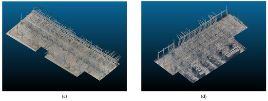
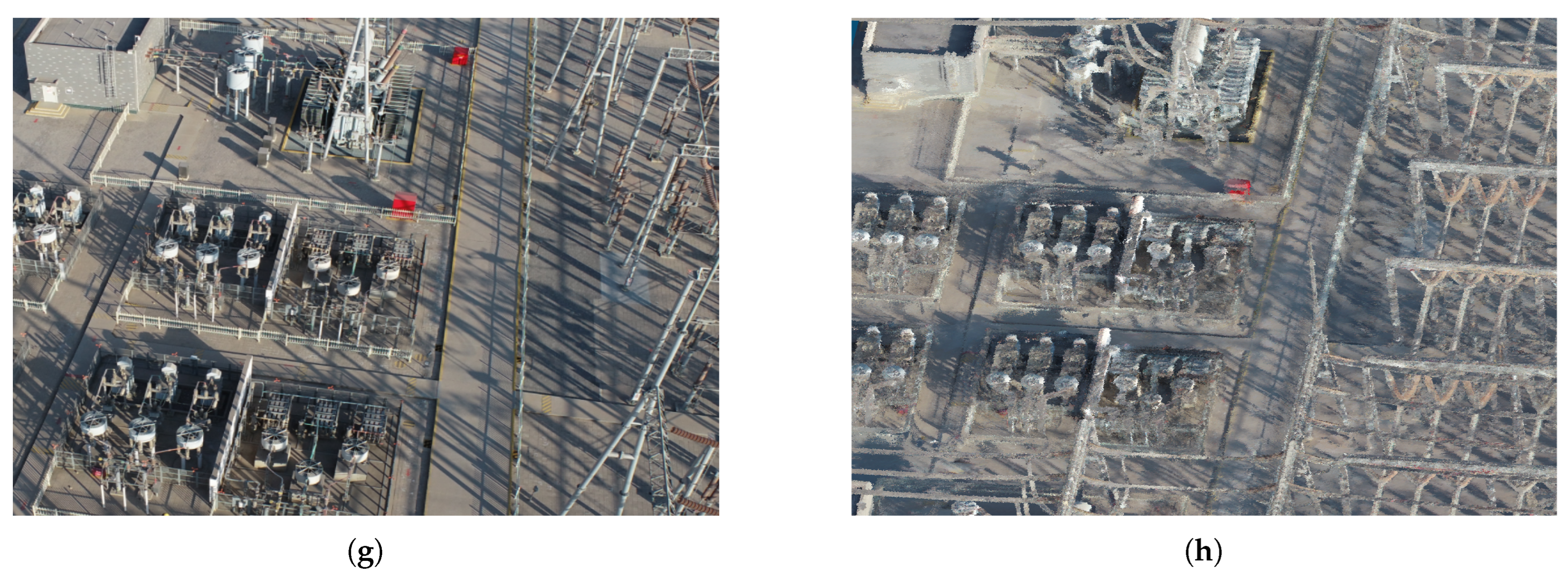
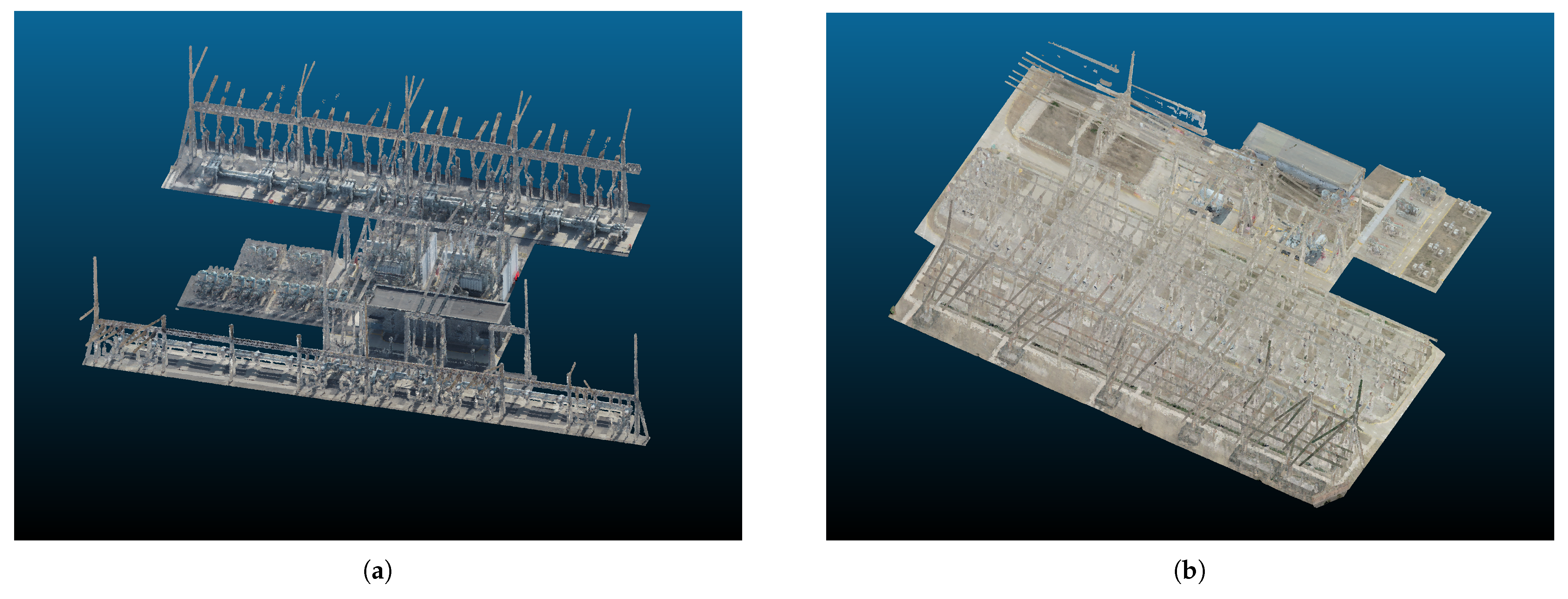
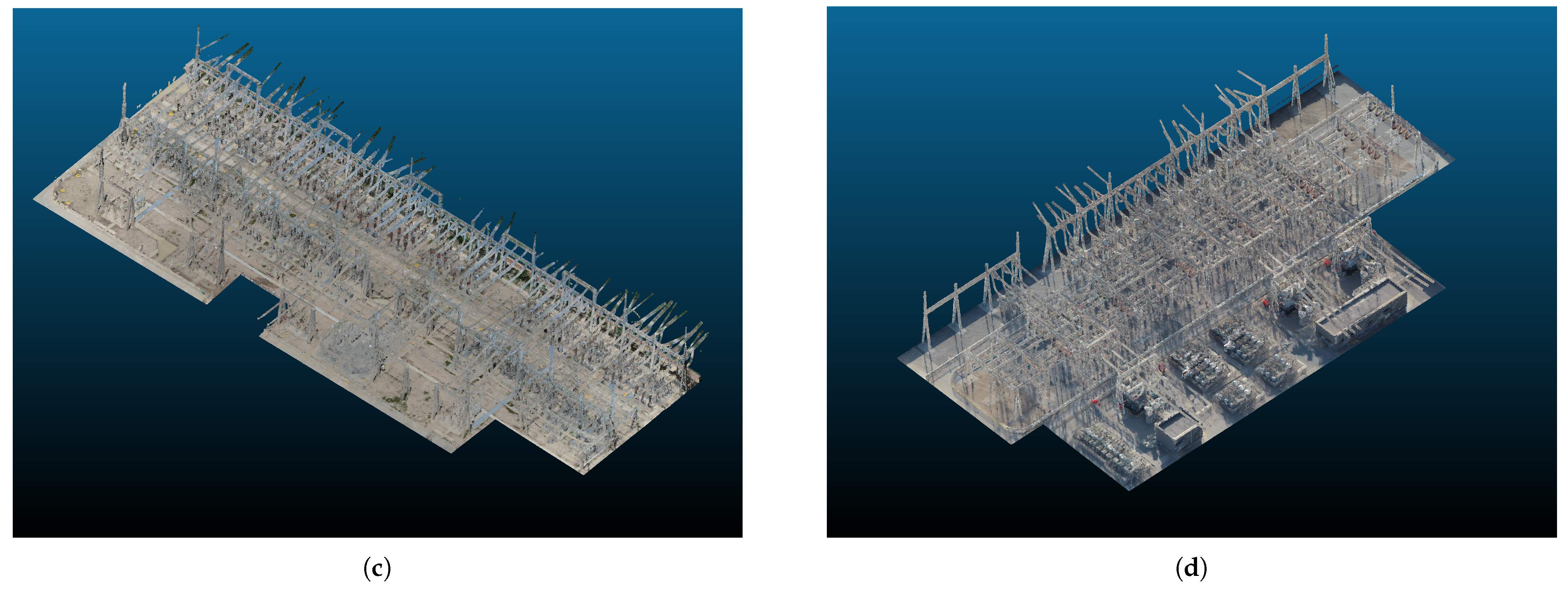
Figure 2.
Overview of four airborne laser-scanned scenes, primarily consisting of insulators, electric wires, bus structures, transformers, and other electrical power equipment. (a–d) represents four different electrical substations.

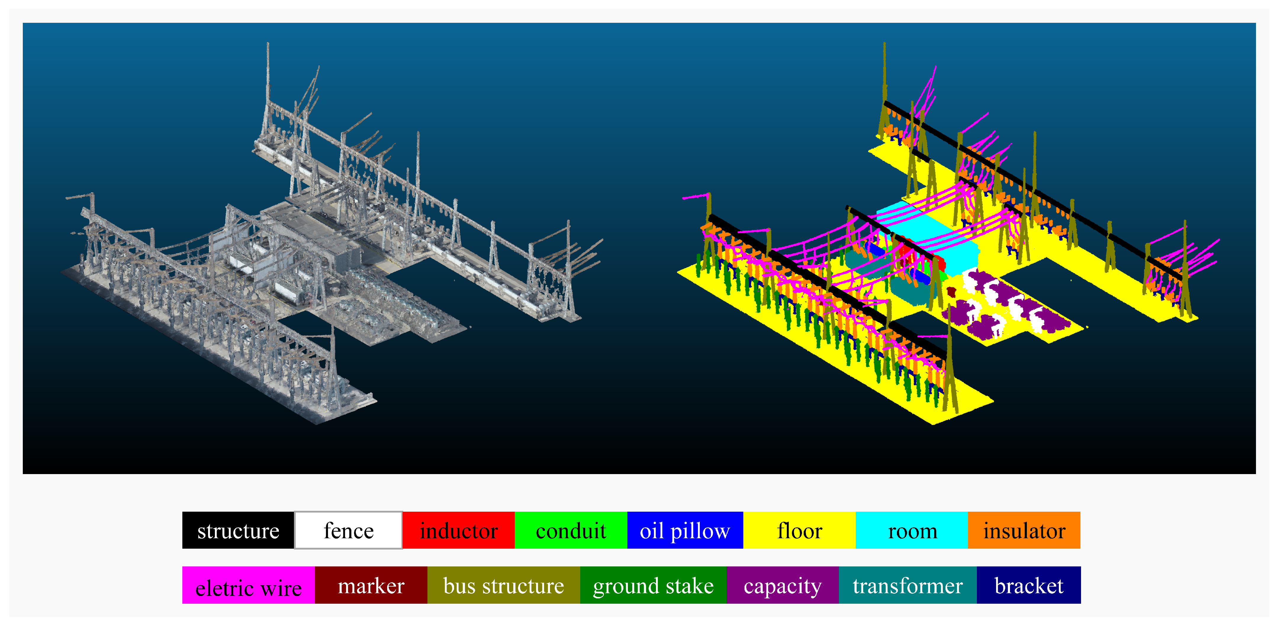
Figure 3.
An example of the original point cloud and the annotated point cloud, where different colors represent different semantic categories.

Table 1.
The number of points of each category within our dataset: Total indicates the number of points of the fifteen categories, while Total* represents the original number of points. M indicates million.
The VCD covers a total area of approximately 90,000 m2. In the true-color point clouds, each point is represented by a six-dimensional vector. This vector integrates spatial information through three dimensions and color information via another three dimensions. Notably, each dimension is susceptible to differing degrees of noise, represented as , , , , , . Given that ∈ represents a point within a noisy true-color point cloud, is defined by Equation (1):
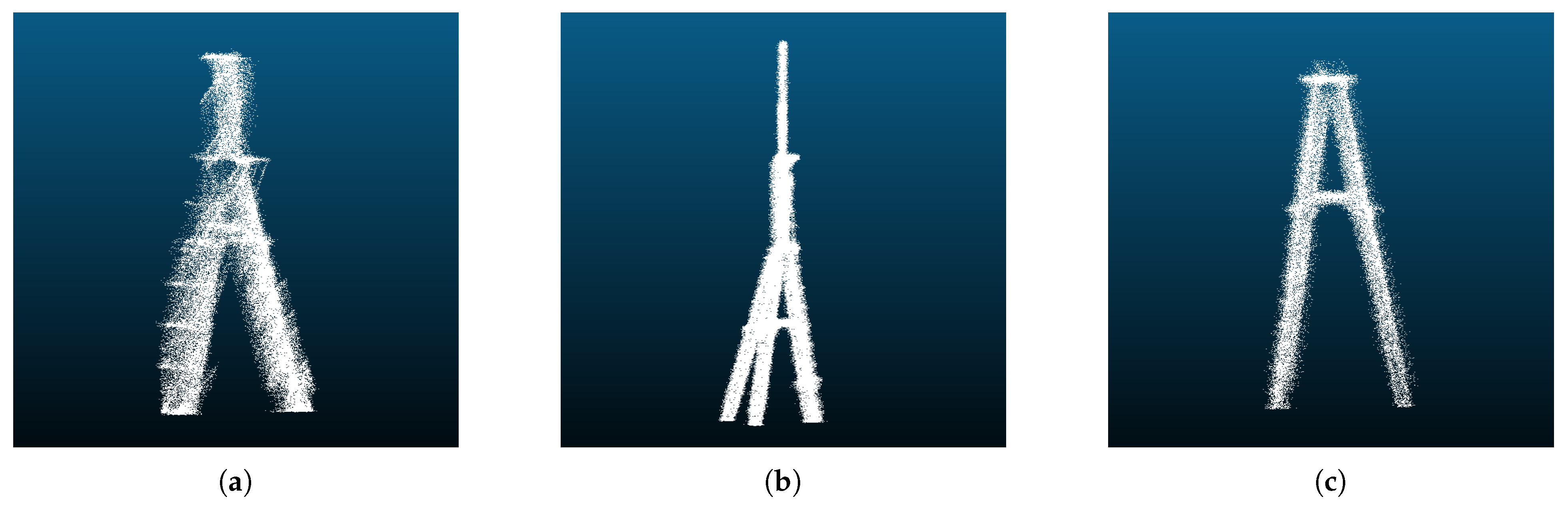
Additionally, the VCD includes a wide array of electrical power equipment commonly found in electrical substations, such as insulators, electric wires, inductors, capacitor banks, distribution rooms, transformers, etc. As shown in Figure 4, there are some geometrically similar objects that belong to different categories. Coupled with the noise introduced by airborne laser scanning (ALS) and the registration of images, these similar objects are difficult to distinguish. Therefore, processing the noisy airborne point clouds is fraught with difficulties.
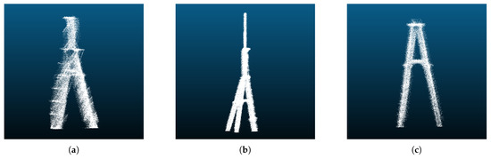
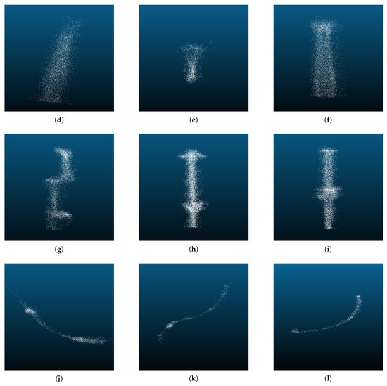
Figure 4.
(a–c): bus structure, (d–f): insulator, (g–i): ground stake, (j–l): electric wire. To better demonstrate the noise and inhomogeneity present in airborne true-color point cloud data, we have modified the RGB coloration of the point cloud to display in white. As shown in figure, objects belonging to the same category exhibit differences in geometric structures (e.g., (a–c)).
3.1.2. Data Annotation
The VCD dataset consists of four large-scale electrical substations and includes 15 categories of important infrastructure within the substations, as shown in Figure 2. Figure 4 displays several annotated samples. Obviously, the use of ALS and the registration of images introduce a significant amount of noise. Furthermore, there are notable geometric differences even among objects of the same label, which poses challenges for the semantic segmentation of such point clouds.
Our point cloud data annotation includes the following steps:
- Spatial Decomposition: we partition each scene into subregions to eliminate irrelevant surrounding objects near the substations, thereby improving processing efficiency.
- Object extraction: substation experts used the advanced point cloud processing software, CloudCompare, to manually extract individual objects within each subregion according to their functional attributes. Subsequently, these segmented objects were stored as distinct files.
- Data quality check: The annotation results are checked by human experts to ensure the high quality and consistency of the annotation of the point cloud data.
3.2. Proposed Novel SSGAM-Net
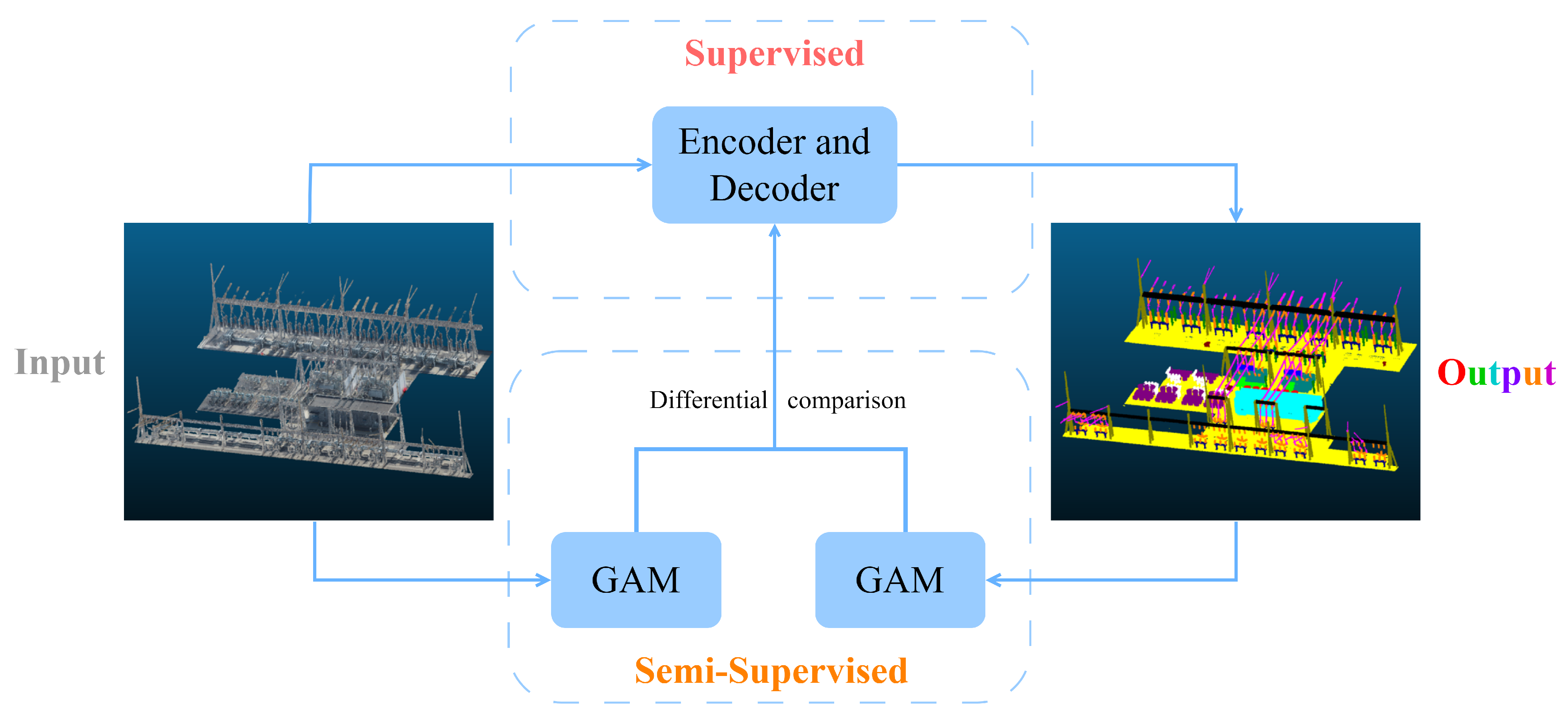
We present an innovative hybrid learning-based network for semantic segmentation of noisy true-color point clouds, named SSGAM-Net. It consists of two primary modules: (1) a GAM module for guiding the network to learn global contextual relationships by generating the pseudo-labels; and (2) an ED module for the extraction of multi-scale features through point convolution. An overview of our proposed SSGAM-Net is presented in Figure 5. As demonstrated by the experimental results in Section IV, the network exhibits better performance on noisy true-color point clouds obtained by drones.

Figure 5.
SSGAM-Net overview.
3.2.1. Semi-Supervised GAM Module
Based on the adjacency relationships between objects, we propose the GAM module, which consists of two parts: (1) the adjacency probability between all pairs of categories; (2) the storage of adjacency probability as an adjacency matrix. The GAM module has demonstrated feasibility, reliability, and interpretability in enhancing the segmentation accuracy of noisy airborne point clouds. In terms of feasibility, adjacency relationships between objects within the point clouds can be measured and calculated through the Euclidean distance or KNN. Regarding reliability, adjacency relationships provide the neural network with global contextual relationships, enhancing the segmentation accuracy of noisy airborne point clouds. In addition, in terms of interpretability, the adjacency relationships between objects enhance the trustworthiness of the network, and the concept of adjacency relationships among objects encapsulates their spatial relationships. Taking the indoor scene as an example, the chair exhibits pronounced spatial relationships with the floor, as opposed to its relatively weaker spatial relationships with the ceiling. In contexts where distinguishing between the ceiling and floor presents a challenge, the spatial contact of the chair with the floor serves as a reference for differentiating against the ceiling. More importantly, the adjacency relationships between objects can be obtained only with a few labeled samples, which allows us to use semi-supervised learning to accelerate the training.
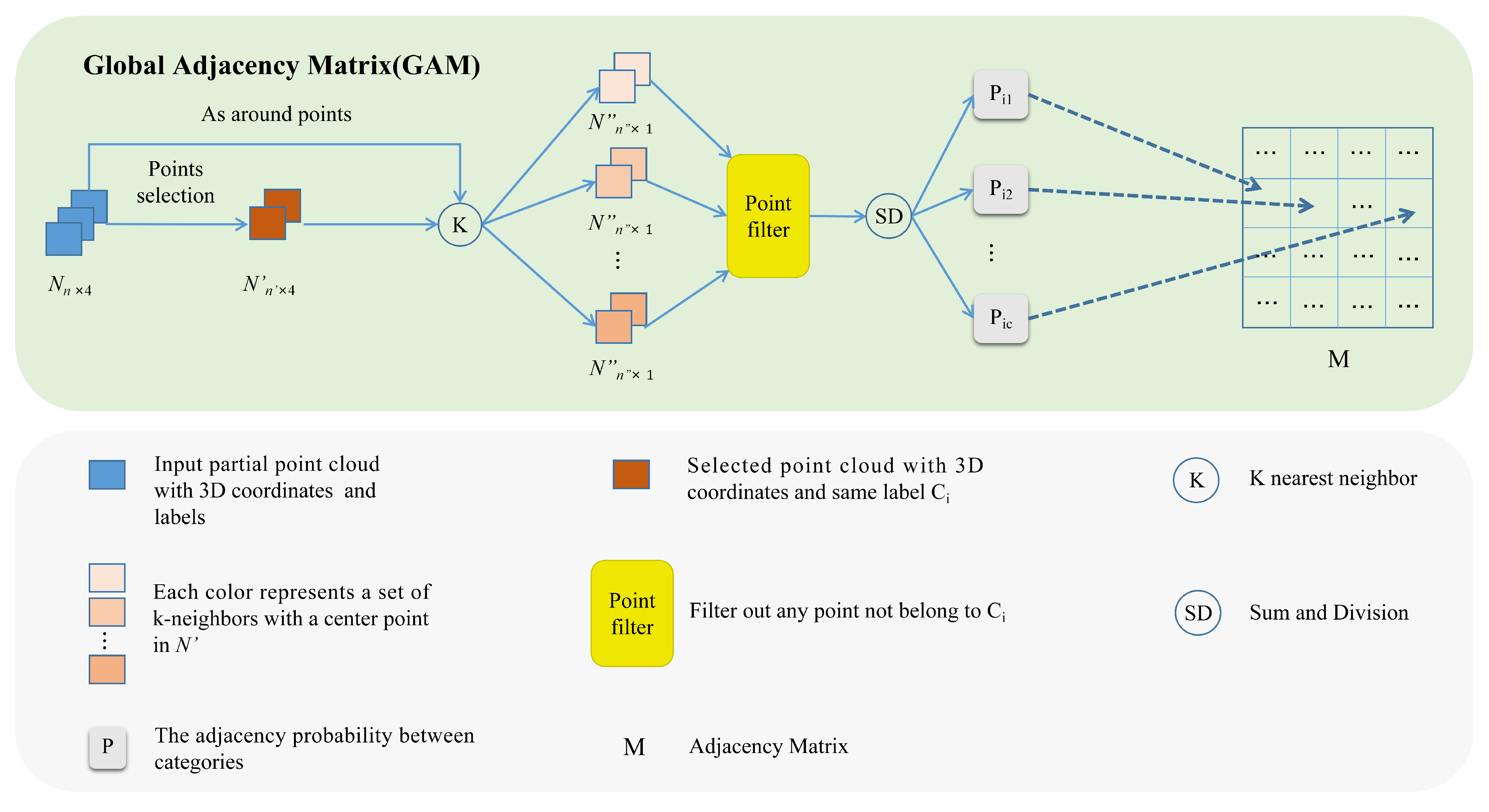
The adjacency relationships between objects are represented as an adjacency matrix M, where each element indicates the adjacency probability between two categories. Specifically, if two categories are adjacent, the corresponding element value in the adjacency matrix will be non-zero; otherwise, it will be zero. As depicted in the GAM module in Figure 6, we use only a few points N to infer global contextual relationships, with each point featuring a three-dimensional coordinate and label in {1, 2, …, C}, where C represents the total number of semantic categories. To obtain the adjacency matrix M, each category label is processed sequentially.
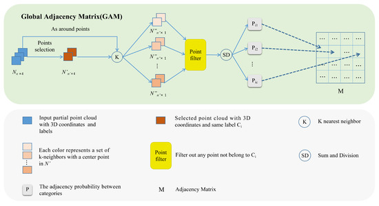
Figure 6.
GAM module.
After selecting the label in N, is obtained. For each center point in , the KNN is used to compute neighboring points, as around points in N, all the neighboring points are named . Among the k neighboring points in , the points with labels different from the central points in are filtered. They are sent to the SD module, and the adjacency probability between the two categories is illustrated in Equation (2).
where is a neighborhood point belonging to , that is, the neighborhood of a center point . is the k-th center point belonging to the i-th category, is the j-th category, and is the number of center points of the i-th category.
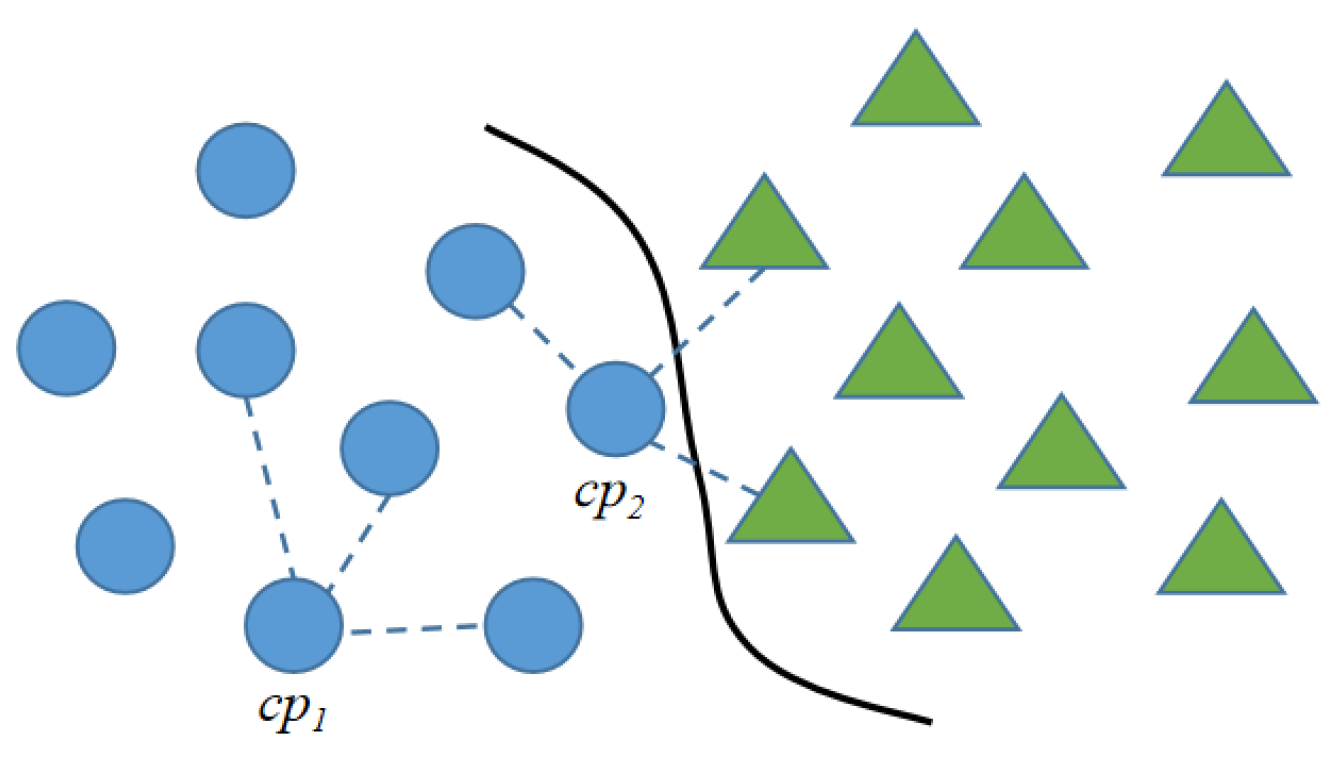
However, in Equation (2), the influence of boundary points on the adjacency probability is greatly underestimated. Regarding the boundary points, a point is defined as a boundary point if its neighborhood contains points of other categories; otherwise, it is defined as an inland point.
As shown in Figure 7, we assume that k = 3, = 3, is the inland point and is the boundary point. When calculating the adjacency probability, should be given a higher weight than , which is called the boundary preference. Since there are far fewer boundary points than inland points, we set a boundary point weight to reinforce the boundary preference, as shown in Equation (3).
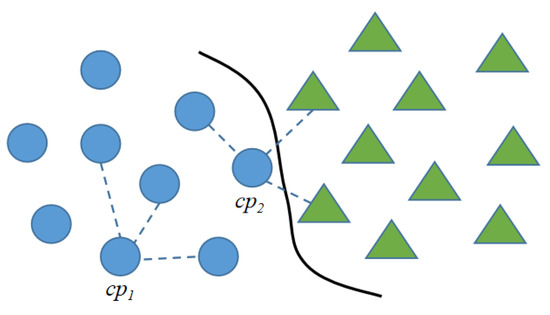
Figure 7.
Illustration of the boundary point effect. Circles and triangles represent two different categories of points.
We propose a novel loss function consisting of two components: (1) , measuring the discrepancy between the output of the Encoder–Decoder module and the ground truth for each point in the prediction results; (2) , assessing the difference between the predicted labels and the pseudo-labels during training. As shown in Figure 8, pseudo-labels are derived from the few labeled data, while the predicted labels are obtained from training. and are compared, and the difference between the two matrices is defined as , as shown in Equation (4). Its value ranges from negative infinity to 1. The closer its value is to negative infinity, the greater the difference between and ; and the closer its value is to 1, the smaller the difference between and . We adopt a logarithmic form of the loss function , as shown in Equation (5).
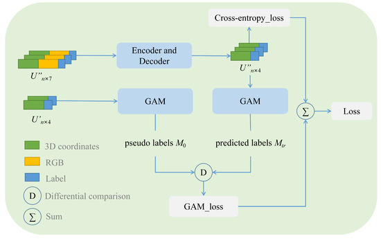
Figure 8.
Combination of segmentation network and GAM module.
The total loss is defined as:
3.2.2. Network Architecture
The overall network architecture is shown in Figure 9, which includes the GAM module and the Encoder–Decoder module. The Encoder module consists of two operations: (1) point convolution-E; (2) aggregation-A. Specifically, for each center point i and its neighboring points , a point convolution operation is used to extract local geometric features . This operation can adaptively adjust and allocate weights within local regions to adapt point clouds of different shapes and densities. Finally, as shown in Equation (7), a max-pooling operation is used to aggregate features relative to the center point i. This operation not only expands the receptive field, but also reduces computational complexity and memory consumption.
where illustrates the distance between the centroid i and its nearest neighbor j; denotes the nearest neighboring points of the centroid i.
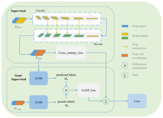
Figure 9.
SSGAM-Net architecture.
In general, the Encoder consists of several point convolution layers, which involve aggregating point features from the neighborhood around a central point. The Decoder’s primary function is to restore the spatial resolution of point clouds. This restoration is achieved by nearest upsampling combined with skip connection to recapture the lost spatial information. After the upsampling stage, the upsampled features are aggregated with those from the corresponding encoder layer. Finally, the network employs a fully connected layer to output the semantic labels. Additionally, in the feature aggregation, SPP is used to merge multi-scale features. SPP executes pooling operations across various levels on feature maps, thereby capturing and aggregating information from multiple scales. At each respective level, SPP divides the feature map into distinct regions, subsequently conducting pooling operations within these regions. Therefore, SPP enables the network to capture both fine-grained local features and coarser-grained global features. This capability facilitates the network’s proficiency in handling objects of diverse sizes and shapes, improving the perception of the network at various scale. With the few labels predicted by the Encoder–Decoder module, the GAM module guides the Encoder–Decoder module to learn the global contextual relationships. Specifically, the Encoder–Decoder module aims to minimize both the and through the application of gradient descent during the training stage.
4. Experiments
4.1. Evaluation Metrics and Experimental Settings
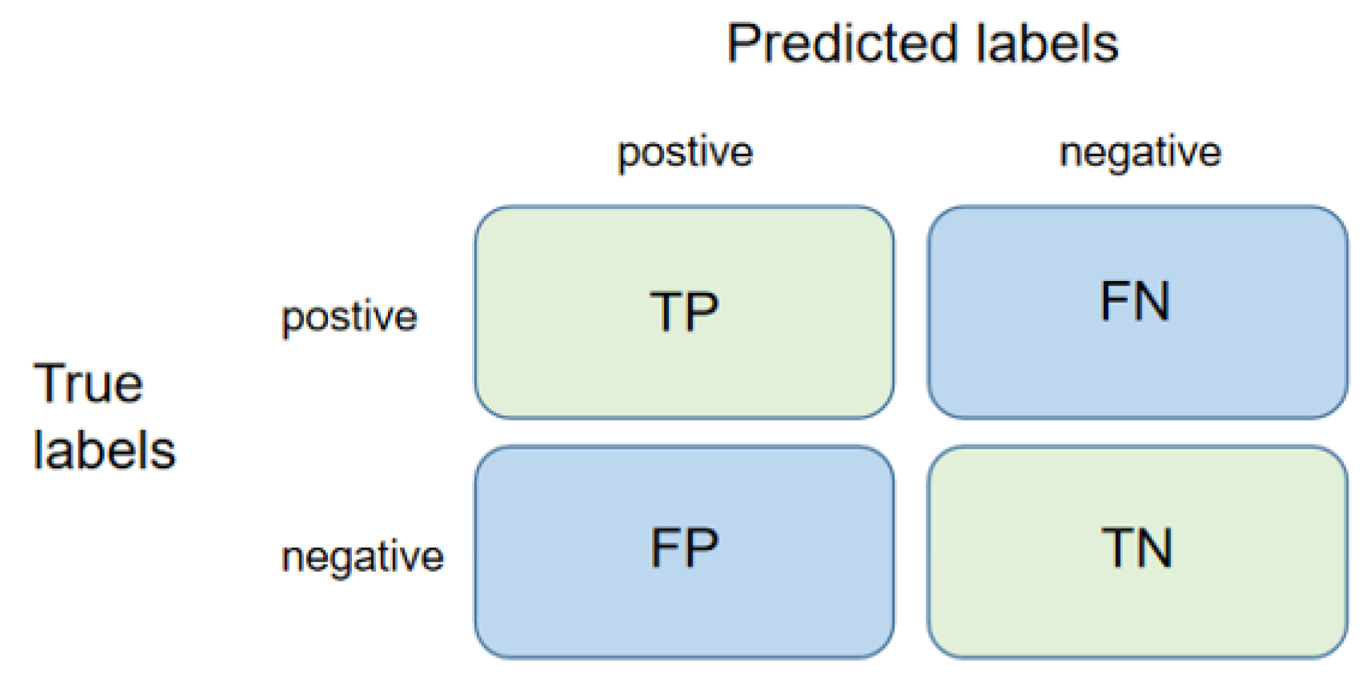
The purpose of point cloud semantic segmentation is to assign semantic labels to individual points within a point cloud. As shown in Figure 10, for each category of points within the prediction results, there are four possible cases: (1) True Positive (TP): this refers to the number of instances in which the model correctly predicted a positive result; (2) False Positive (FP): this denotes the number of instances in which the model erroneously predicted a positive result; (3) False Negative (FN): this represents the number of instances in which the model mistakenly predicted a negative result; (4) True Negative (TN): this refers to the number of instances where the model accurately predicted a negative result.
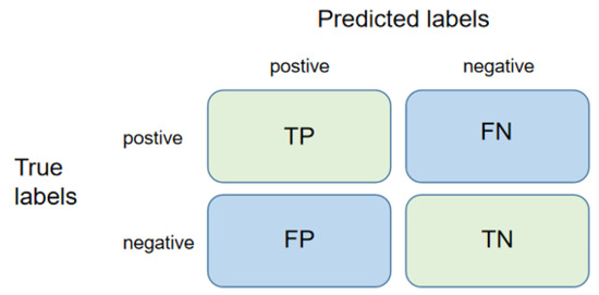
Figure 10.
Typical confusion matrix.
Intersection over union (IoU) and overall accuracy (OA) are commonly used evaluation metrics in point cloud semantic segmentation. IoU is calculated as the proportion of intersection and union between the predicted segmentation results and the ground truth. A higher IoU indicates that neural networks predict more accurate segmentation boundaries. The mean IoU (mIoU) is the average value of IoUs for all categories. The OA metric measures the classification accuracy of model, calculated as the proportion of correctly classified points and the total number of points. A higher OA indicates that neural networks have better segmentation performance. The above metrics are shown in Equations (8)–(10):
In summary, we use the above metrics to evaluate the performance of the neural network in the following experiments.
4.2. Experimental Settings and Environment
We conduct experiments on VCD. This experimental dataset consists of 15 categories of industrial objects. During the training process, we set the number of neighboring points k at 1500, and the weight of is assigned as 25. In addition, we set the batch size at 6, the learning rate at 0.001, and the number of training epochs at 50, with the Adam optimizer. In order to improve computational efficiency, downsampling is required, while simultaneously preserving the adjacency relationships. Therefore, we implement a global uniform downsampling strategy in each training scene for the computation of the GAM. In the following comparative experiments, the primary parameters for each method are defined as follows. For RandLA-Net and BAAF-Net, the k value in KNN algorithm is set to 16. Both methods utilize an input of 40,960 points and a sub-grid size of 0.04. In the case of KPConv and RRDAN, the number of kernel points is set at 15. KPConv employs a input sphere radius of 3.0 for the input sphere, a first subsampling grid size of 0.06, and a convolution radius of 2.5. RRDAN uses an input sphere radius of 20 and a first subsampling grid size of 0.40, and maintains the same convolution radius of 2.5. The number of input points for both PointNet and PointNet++ is 4096. All training and testing are conducted on the same equipment.
4.3. Experimental Results
4.3.1. Comparison with Other Methods
In Table 2, our method outperforms current advanced methods in both mIoU and global OA metrics, particularly in mIoU. Compared to the other methods, our approach has improved 4.2% in mIoU. Our method exhibits competitive performance in the semantic segmentation of airborne noisy true-color point clouds. Notably, for category pairs with similar shapes, such as insulators and ground stakes, capacitors and inductors, and small-sized objects such as brackets and conduits, our method shows a significant advantage over other methods. The aforementioned advantages indicate that the adjacency relationships between objects captured by the GAM module significantly improve the performance of the network. Specifically, our proposed method is capable of accurately segmenting key objects in UAV electrical power inspection, offering significant value for industrial applications.
Table 2.
Comparison of segmentation results between the proposed SSGAM-Net and other methods.
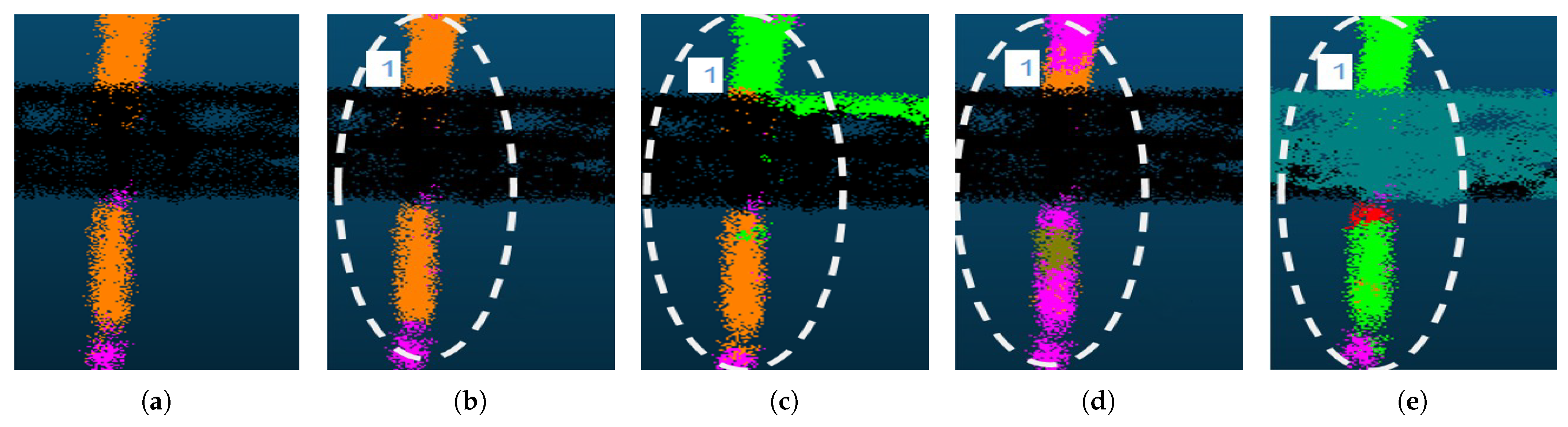
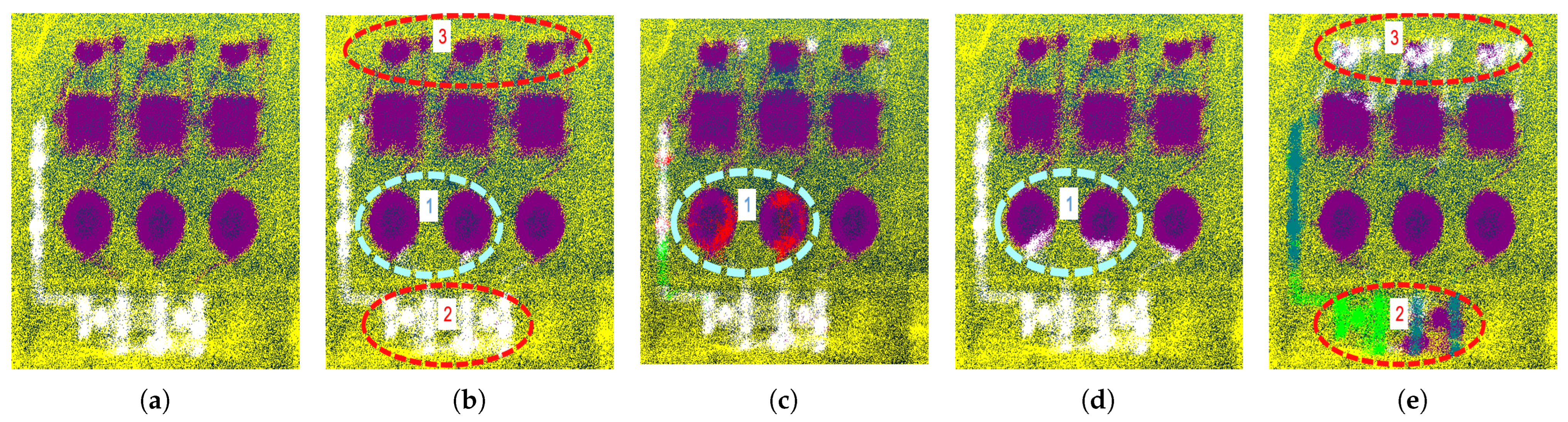
The GAM module performs well in different scale regions by taking advantage of minimizing both and . In small-scale region No. 1 of Figure 11, all methods except (b) SSGAM-Net exhibit different degrees of mis-segmentation. SSGAM-Net performs well because of the powerful GAM module, which guides the network to learn global contextual relationships within noisy point clouds, avoiding the mis-segmentation of non-adjacent objects existing in the same local space. In the large-scale region, as shown in Figure 12, region No. 1 in (c,d), and regions No. 2 and 3 in (e) all exhibit mis-segmentation of non-adjacent objects existing in the same local space. However, benefiting from the pseudo-label guidance of the powerful GAM module, (b) SSGAM-Net still performs well in regions No. 1, 2, and 3. The results show that the GAM module effectively guides the network to learn global contextual relationships within noisy point clouds by generating pseudo-labels, which dramatically improves the segmentation accuracy. The prevents non-adjacent objects of different categories from being mis-segmented into the same local space, while the reduces the risk of mis-segmentation of the entire object.
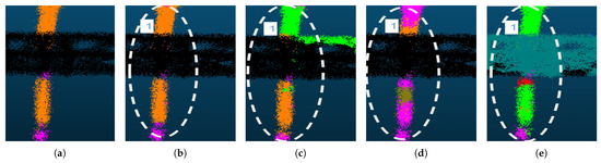
Figure 11.
The segmentation results of the insulator on the structure in small-scale regions. (a) Ground truth; (b) SSGAM-Net; (c) BAAF-Net; (d) KPConv; (e) RandLA-Net. The dashed ellipse region indicates region No. 1.
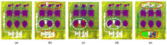
Figure 12.
The segmentation result of the capacitor in large-scale regions. (a) Ground truth; (b) SSGAM-Net; (c) BAAF-Net; (d) KPConv; (e) RandLA-Net. The dashed ellipse regions indicate the corresponding numbered regions.
4.3.2. Hyperparameter Selection
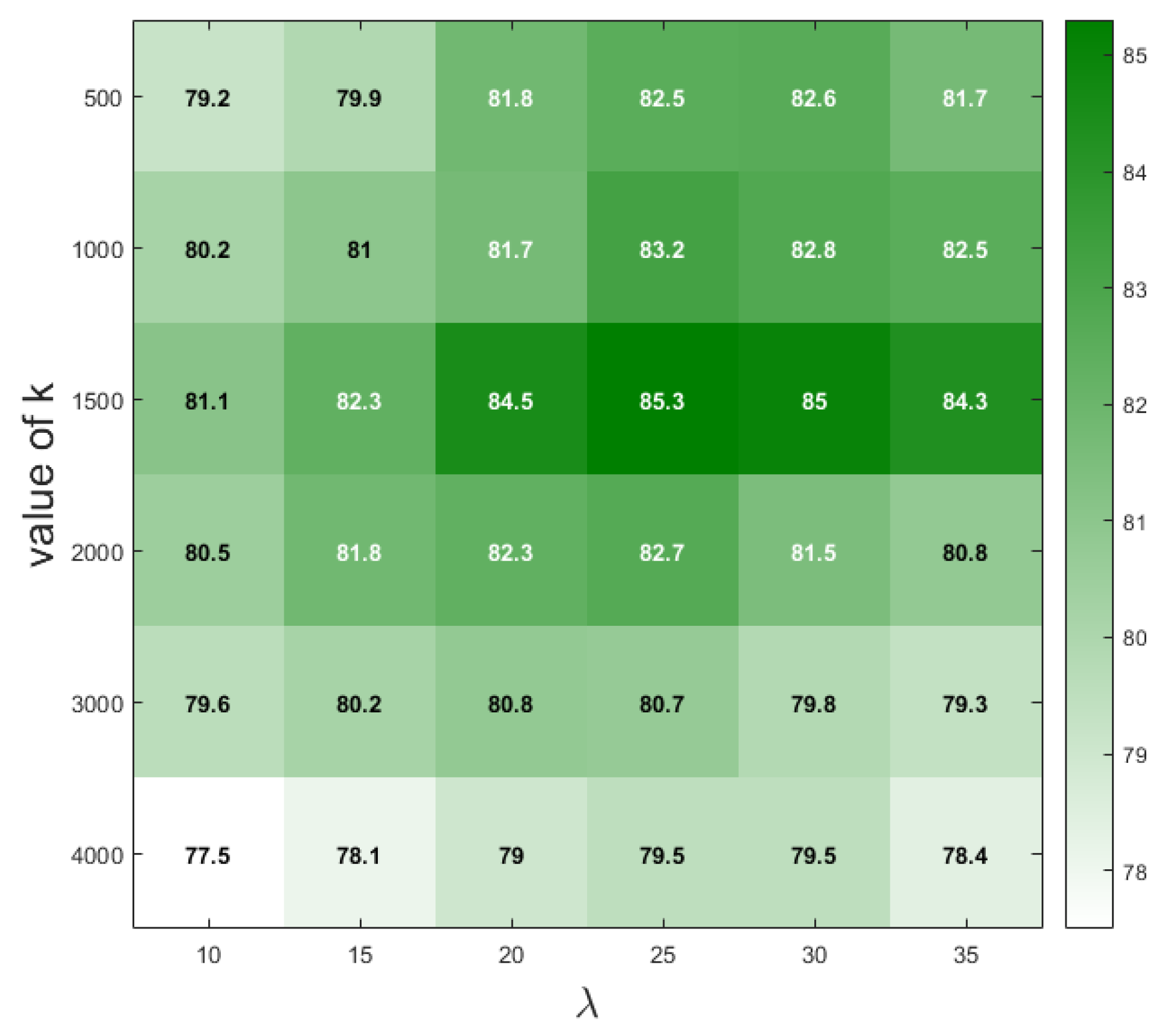
To determine the suitable values of the hyperparameters k and of the GAM module in the experiments, we empirically set 36 different combinations of k and values, and determine the appropriate values based on mIoU. The experimental results are shown in Figure 13; when the value of k is close to 1500 and the value of is close to 25, the segmentation results on the VCD achieve the best mIoU. Based on the experimental facts, we adopt the set of hyperparameters k = 1500 and = 25 when conducting experiments on VCD.
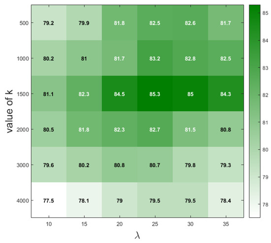
Figure 13.
The experimental results are under different combinations of k and values. The darker the color, the higher the mIoU under the corresponding hyperparameter combination, and the values inside each square indicate the mIoU.
4.3.3. Computational Cost Comparison
Furthermore, a comparative analysis was conducted on the computational time and memory consumption among various methods during training. Batch size is uniformly set to 6. The data presented in Table 3 indicate that PointNet and RandLA-Net demonstrate the fastest processing time. On the contrary, PointNet++ exhibits the most prolonged processing time, consuming 5182 s per epoch. Notably, despite RandLA-Net’s remarkably fast processing time of 98 s per epoch, it consumes substantial GPU memory cost, amounting to 23,282 MB. This shows that RandLA-Net necessitates considerable memory resources to handle large-scale data, while it is time-efficient. KPConv demonstrates good performance in terms of processing efficiency and GPU memory utilization. After the above quantitative comparison, our proposed SSGAM-Net shows advantages in higher accuracy and acceptable GPU memory cost for time-insensitive tasks such as offline segmentation.
Table 3.
The processing time and memory consumption among various methods during training.
5. Conclusions and Outlook
In this paper, we present a novel hybrid semi-supervised and supervised network, SSGAM-Net, for semantic segmentation of noisy true-color point clouds obtained by drones. Without the need for redundant pre-processing or post-processing, our proposed method provides an elegant and efficient way for direct semantic segmentation of airborne noisy point clouds. To verify the performance of SSGAM-Net, we built an airborne industrial true-color point cloud dataset VCD for the experiments. The experimental results on VCD show that our proposed method achieves 85.3% in mIoU and 96.6% in OA. Specifically, in terms of the metric mIoU, our SSGAM-Net surpasses other advanced algorithms by a margin of 4.2 to 58%, achieving a competitive level. Moreover, the results validate not only that the pseudo-labels generated by the GAM module in semi-supervised settings correctly represent the adjacency relationships between objects, but also that pseudo-labels effectively guide the network to learn the global contextual relationships within noisy point clouds. Benefiting from the powerful GAM module, the ED module is able to utilize the global contextual relationships to improve the segmentation performance. Therefore, our proposed SSGAM-Net is suitable for direct semantic segmentation of airborne noisy true-color point clouds, exhibiting significant potential for application in intelligent industrial O&M.
Our work introduces a new perspective for understanding global contextual relationships within noisy point clouds, effectively linking global contextual relationships to concrete adjacency relationships. The adjacency relationships serve as a vital reference to distinguish between objects that share similar features, such as geometry or color information. Therefore, it considerably enhances the explainability and trustworthiness of the model.
In this work, we are the first to characterize the spatial relationships of components in industrial scenarios and combine them with a novel hybrid learning framework to accurately segment airborne noisy true-color point clouds. However, our proposed method is unable to temporarily support multimodal data and has not yet conducted model lightweighting. In future work, we will focus on lightweighting the network so that it can be efficiently deployed in edge devices for intelligent industrial O&M applications, such as the construction and updating of industrial BIM models. Moreover, we will aim to enhance the model’s ability to process multimodal data.
Author Contributions
Conceptualization, H.W. and Z.H.; methodology, H.W., Z.H., and W.Z.; software, Z.H. and W.Z.; validation, H.W., Z.H. and W.Z.; writing—original draft preparation, H.W, Z.H., and W.Z.; writing—review and editing, H.W., Z.H., W.Z., X.B., L.S., and M.P.; funding acquisition, H.W., X.B., L.S., and M.P. All authors have read and agreed to the published version of the manuscript.
Funding
This research was jointly supported by the National Natural Science Foundation of China(62202164, 62301220), and the Fundamental Research Funds for the Central Universities (2021MS016).
Data Availability Statement
The data supporting the findings of this research are available from the corresponding author upon reasonable request. The data are not publicly available due to ongoing use by the data holders and stakeholders.
Conflicts of Interest
The authors declare no conflicts of interest.
References
- Zhang, J.; Sun, Z.; Sun, J. 3-DFineRec: Fine-Grained Recognition for Small-Scale Objects in 3-D Point Cloud Scenes. IEEE Trans. Instrum. Meas. 2021, 71, 5000312. [Google Scholar] [CrossRef]
- Qi, C.; Yin, J. Multigranularity Semantic Labeling of Point Clouds for the Measurement of the Rail Tanker Component with Structure Modeling. IEEE Trans. Instrum. Meas. 2020, 70, 5000312. [Google Scholar] [CrossRef]
- Yuan, Q.; Luo, Y.; Wang, H. 3D point cloud recognition of substation equipment based on plane detection. Results Eng. 2022, 15, 100545. [Google Scholar] [CrossRef]
- Shen, X.; Xu, Z.; Wang, M. An Intelligent Point Cloud Recognition Method for Substation Equipment Based on Multiscale Self-Attention. IEEE Trans. Instrum. Meas. 2023, 72, 2528912. [Google Scholar] [CrossRef]
- Arastounia, M.; Lichti, D.D. Automatic Object Extraction from Electrical Substation Point Clouds. Remote Sens. 2015, 7, 15605–15629. [Google Scholar] [CrossRef]
- Wu, Q.; Yang, H.; Wei, M.; Remil, O.; Wang, B.; Wang, J. Automatic 3D reconstruction of electrical substation scene from LiDAR point cloud. ISPRS J. Photogramm. Remote Sens. 2018, 143, 57–71. [Google Scholar] [CrossRef]
- Jeong, S.; Kim, D.; Kim, S.; Ham, J.W.; Lee, J.K.; Oh, K.Y. Real-Time Environmental Cognition and Sag Estimation of Transmission Lines Using UAV Equipped With 3-D Lidar System. IEEE Trans. Power Deliv. 2020, 36, 2658–2667. [Google Scholar] [CrossRef]
- Chakravarthy, A.S.; Sinha, S.; Narang, P.; Mandal, M.; Chamola, V.; Yu, F.R. DroneSegNet: Robust Aerial Semantic Segmentation for UAV-Based IoT Applications. IEEE Trans. Veh. Technol. 2022, 71, 4277–4286. [Google Scholar] [CrossRef]
- Pepe, M.; Alfio, V.S.; Costantino, D.; Scaringi, D. Data for 3D reconstruction and point cloud classification using machine learning in cultural heritage environment. Data Brief 2022, 42, 108250. [Google Scholar] [CrossRef]
- Romero-Jarén, R.; Arranz, J. Automatic segmentation and classification of BIM elements from point clouds. Autom. Constr. 2021, 124, 103576. [Google Scholar] [CrossRef]
- Ma, J.W.; Czerniawski, T.; Leite, F. Semantic segmentation of point clouds of building interiors with deep learning: Augmenting training datasets with synthetic BIM-based point clouds. Autom. Constr. 2020, 113, 103144. [Google Scholar] [CrossRef]
- Gao, H.; Koch, C.; Wu, Y. Building information modelling based building energy modelling: A review. Appl. Energy 2019, 238, 320–343. [Google Scholar] [CrossRef]
- Štroner, M.; Urban, R.; Línková, L. A New Method for UAV Lidar Precision Testing Used for the Evaluation of an Affordable DJI ZENMUSE L1 Scanner. Remote Sens. 2021, 13, 4811. [Google Scholar] [CrossRef]
- Guo, Y.; Wang, H.; Hu, Q.; Liu, H.; Liu, L.; Bennamoun, M. Deep Learning for 3D Point Clouds: A Survey. IEEE Trans. Pattern Anal. Mach. Intell. 2020, 43, 4338–4364. [Google Scholar] [CrossRef]
- Diara, F.; Roggero, M. Quality Assessment of DJI Zenmuse L1 and P1 LiDAR and Photogrammetric Systems: Metric and Statistics Analysis with the Integration of Trimble SX10 Data. Geomatics 2022, 2, 254–281. [Google Scholar] [CrossRef]
- Zhang, J.; Lin, X.; Ning, X. SVM-Based Classification of Segmented Airborne LiDAR Point Clouds in Urban Areas. Remote Sens. 2013, 5, 3749–3775. [Google Scholar] [CrossRef]
- Grandio, J.; Riveiro, B.; Soilán, M.; Arias, P. Point cloud semantic segmentation of complex railway environments using deep learning. Autom. Constr. 2022, 141, 104425. [Google Scholar] [CrossRef]
- Xia, T.; Yang, J.; Chen, L. Automated semantic segmentation of bridge point cloud based on local descriptor and machine learning. Autom. Constr. 2022, 133, 103992. [Google Scholar] [CrossRef]
- Xia, X.; Meng, Z.; Han, X.; Li, H.; Tsukiji, T.; Xu, R.; Zheng, Z.; Ma, J. An automated driving systems data acquisition and analytics platform. Transp. Res. Part C Emerg. Technol. 2023, 151, 104120. [Google Scholar] [CrossRef]
- Meng, Z.; Xia, X.; Xu, R.; Liu, W.; Ma, J. HYDRO-3D: Hybrid Object Detection and Tracking for Cooperative Perception Using 3D LiDAR. IEEE Trans. Intell. Veh. 2023, 8, 4069–4080. [Google Scholar] [CrossRef]
- Zhou, Y.; Ji, A.; Zhang, L.; Xue, X. Sampling-attention deep learning network with transfer learning for large-scale urban point cloud semantic segmentation. Eng. Appl. Artif. Intell. 2023, 117, 105554. [Google Scholar] [CrossRef]
- Liu, C.; Zeng, D.; Akbar, A.; Wu, H.; Jia, S.; Xu, Z.; Yue, H. Context-aware network for semantic segmentation toward large-scale point clouds in urban environments. IEEE Trans. Geosci. Remote Sens. 2022, 60, 1–15. [Google Scholar] [CrossRef]
- Tatarchenko, M.; Park, J.; Koltun, V.; Zhou, Q.Y. Tangent Convolutions for Dense Prediction in 3D. In Proceedings of the 2018 IEEE/CVF Conference on Computer Vision and Pattern Recognition (CVPR), Salt Lake City, UT, USA, 18–22 June 2018; pp. 3887–3896. [Google Scholar]
- Wu, B.; Zhou, X.; Zhao, S.; Yue, X.; Keutzer, K. Squeezesegv2: Improved Model Structure and Unsupervised Domain Adaptation for Road-Object Segmentation from a LiDAR Point Cloud. In Proceedings of the 2019 International Conference on Robotics and Automation (ICRA), Montreal, QC, Canada, 20–24 May 2019; pp. 4376–4382. [Google Scholar]
- Zhang, Y.; Zhou, Z.; David, P.; Yue, X.; Xi, Z.; Gong, B.; Foroosh, H. PolarNet: An Improved Grid Representation for Online LiDAR Point Clouds Semantic Segmentation. In Proceedings of the 2020 IEEE/CVF Conference on Computer Vision and Pattern Recognition (CVPR), Seattle, WA, USA, 14–19 June 2020; pp. 9601–9610. [Google Scholar]
- Razani, R.; Cheng, R.; Taghavi, E.; Bingbing, L. Lite-HDSeg: LiDAR Semantic Segmentation Using Lite Harmonic Dense Convolutions. In Proceedings of the 2021 IEEE International Conference on Robotics and Automation (ICRA), Xi’an, SX, China, 30 May–5 June 2021; pp. 9550–9556. [Google Scholar]
- Milioto, A.; Vizzo, I.; Behley, J.; Stachniss, C. RangeNet++: Fast and Accurate LiDAR Semantic Segmentation. In Proceedings of the 2019 IEEE/RSJ International Conference on Intelligent Robots and Systems (IROS), Macau, China, 3–8 November 2019; pp. 4213–4220. [Google Scholar]
- Zhou, Y.; Tuzel, O. VoxelNet: End-to-End Learning for Point Cloud Based 3D Object Detection. In Proceedings of the 2018 IEEE/CVF Conference on Computer Vision and Pattern Recognition (CVPR), Salt Lake City, UT, USA, 18–22 June 2018; pp. 4490–4499. [Google Scholar]
- Riegler, G.; Osman Ulusoy, A.; Geiger, A. OctNet: Learning Deep 3D Representations at High Resolutions. In Proceedings of the 2017 IEEE/CVF Conference on Computer Vision and Pattern Recognition (CVPR), Honolulu, HI, USA, 21–26 July 2017; pp. 3577–3586. [Google Scholar]
- Meng, H.Y.; Gao, L.; Lai, Y.K.; Manocha, D. VV-Net: Voxel VAE Net With Group Convolutions for Point Cloud Segmentation. In Proceedings of the 2019 IEEE/CVF International Conference on Computer Vision (ICCV), Seoul, Republic of Korea, 27 October–2 November 2019; pp. 8500–8508. [Google Scholar]
- Liu, Z.; Tang, H.; Lin, Y.; Han, S. Point-Voxel CNN for Efficient 3D Deep Learning. In Proceedings of the Advances in Neural Information Processing Systems (NeurIPS), Vancouver, BC, Canada, 8–14 December 2019. [Google Scholar]
- Qi, C.R.; Su, H.; Mo, K.; Guibas, L.J. PointNet: Deep Learning on Point Sets for 3D Classification and Segmentation. In Proceedings of the 2017 IEEE/CVF Conference on Computer Vision and Pattern Recognition (CVPR), Honolulu, HI, USA, 21–26 July 2017; pp. 652–660. [Google Scholar]
- Qi, C.R.; Yi, L.; Su, H.; Guibas, L.J. Pointnet++: Deep Hierarchical Feature Learning on Point Sets in a Metric Space. In Proceedings of the Advances in Neural Information Processing Systems (NeurIPS), Long Beach, CA, USA, 4–9 December 2017. [Google Scholar]
- Zhao, H.; Jiang, L.; Fu, C.W.; Jia, J. PointWeb: Enhancing Local Neighborhood Features for Point Cloud Processing. In Proceedings of the 2019 IEEE/CVF Conference on Computer Vision and Pattern Recognition (CVPR), Long Beach, CA, USA, 16–20 June 2019; pp. 5565–5573. [Google Scholar]
- Zhang, Z.; Hua, B.S.; Yeung, S.K. ShellNet: Efficient Point Cloud Convolutional Neural Networks Using Concentric Shells Statistics. In Proceedings of the 2019 IEEE/CVF International Conference on Computer Vision (ICCV), Seoul, Republic of Korea, 27 October–2 November 2019; pp. 1607–1616. [Google Scholar]
- Hu, Q.; Yang, B.; Xie, L.; Rosa, S.; Guo, Y.; Wang, Z.; Trigoni, N.; Markham, A. RandLA-Net: Efficient Semantic Segmentation of Large-Scale Point Clouds. In Proceedings of the 2020 IEEE/CVF Conference on Computer Vision and Pattern Recognition (CVPR), Seattle, WA, USA, 14–19 June 2020; pp. 11105–11114. [Google Scholar]
- Li, Y.; Bu, R.; Sun, M.; Wu, W.; Di, X.; Chen, B. PointCNN: Convolution On X-Transformed Points. In Proceedings of the Advances in Neural Information Processing Systems (NeurIPS), Montreal, QC, Canada, 3–8 December 2018. [Google Scholar]
- Komarichev, A.; Zhong, Z.; Hua, J. A-CNN: Annularly Convolutional Neural Networks on Point Clouds. In Proceedings of the 2019 IEEE/CVF Conference on Computer Vision and Pattern Recognition (CVPR), Long Beach, CA, USA, 16–20 June 2019; pp. 7421–7430. [Google Scholar]
- Wang, S.; Suo, S.; Ma, W.C.; Pokrovsky, A.; Urtasun, R. Deep Parametric Continuous Convolutional Neural Networks. In Proceedings of the 2018 IEEE/CVF Conference on Computer Vision and Pattern Recognition (CVPR), Salt Lake City, UT, USA, 18–22 June 2018; pp. 2589–2597. [Google Scholar]
- Thomas, H.; Qi, C.R.; Deschaud, J.E.; Marcotegui, B.; Goulette, F.; Guibas, L. KPConv: Flexible and Deformable Convolution for Point Clouds. In Proceedings of the 2019 IEEE/CVF International Conference on Computer Vision (ICCV), Seoul, Republic of Korea, 27 October–2 November 2019; pp. 6410–6419. [Google Scholar]
- Zeng, T.; Luo, F.; Guo, T.; Gong, X.; Xue, J.; Li, H. Recurrent Residual Dual Attention Network for Airborne Laser Scanning Point Cloud Semantic Segmentation. IEEE Trans. Geosci. Remote Sens. 2023, 61, 5702614. [Google Scholar] [CrossRef]
- Lin, Y.; Vosselman, G.; Cao, Y.; Yang, M.Y. Local and global encoder network for semantic segmentation of Airborne laser scanning point clouds. ISPRS J. Photogramm. Remote Sens. 2021, 176, 151–168. [Google Scholar] [CrossRef]
- Liu, W.; Quijano, K.; Crawford, M.M. YOLOv5-Tassel: Detecting Tassels in RGB UAV Imagery With Improved YOLOv5 Based on Transfer Learning. IEEE J. Sel. Top. Appl. Earth Obs. Remote Sens. 2022, 15, 8085–8094. [Google Scholar] [CrossRef]
- Dharmadasa, V.; Kinnard, C.; Baraër, M. An Accuracy Assessment of Snow Depth Measurements in Agro-forested Environments by UAV Lidar. Remote Sens. 2022, 14, 1649. [Google Scholar] [CrossRef]
- Kim, M.; Stoker, J.; Irwin, J.; Danielson, J.; Park, S. Absolute Accuracy Assessment of Lidar Point Cloud Using Amorphous Objects. Remote Sens. 2022, 14, 4767. [Google Scholar] [CrossRef]
- Qiu, S.; Anwar, S.; Barnes, N. Semantic Segmentation for Real Point Cloud Scenes via Bilateral Augmentation and Adaptive Fusion. In Proceedings of the 2021 IEEE/CVF Conference on Computer Vision and Pattern Recognition (CVPR), Virtual, 19–25 June 2021; pp. 1757–1767. [Google Scholar]
- Wu, W.; Qi, Z.; Fuxin, L. PointConv: Deep Convolutional Networks on 3D Point Clouds. In Proceedings of the 2019 IEEE/CVF Conference on Computer Vision and Pattern Recognition (CVPR), Long Beach, CA, USA, 16–20 June 2019; pp. 9613–9622. [Google Scholar]
- Mao, J.; Wang, X.; Li, H. Interpolated Convolutional Networks for 3D Point Cloud Understanding. In Proceedings of the 2019 IEEE/CVF International Conference on Computer Vision (ICCV), Seoul, Republic of Korea, 27 October–2 November 2019; pp. 1578–1587. [Google Scholar]
- Armeni, I.; Sax, S.; Zamir, A.R.; Savarese, S. Joint 2D-3D-Semantic Data for Indoor Scene Understanding. arXiv 2017, arXiv:1702.01105. [Google Scholar]
- Dai, A.; Chang, A.X.; Savva, M.; Halber, M.; Funkhouser, T.; Nießner, M. ScanNet: Richly-Annotated 3D Reconstructions of Indoor Scenes. In Proceedings of the 2017 IEEE/CVF Conference on Computer Vision and Pattern Recognition (CVPR), Honolulu, HI, USA, 21–26 July 2017; pp. 2432–2443. [Google Scholar]
- Wu, Z.; Song, S.; Khosla, A.; Yu, F.; Zhang, L.; Tang, X.; Xiao, J. 3D ShapeNets: A Deep Representation for Volumetric Shapes. In Proceedings of the 2015 IEEE Conference on Computer Vision and Pattern Recognition (CVPR), Boston, MA, USA, 7–12 June 2015; pp. 1912–1920. [Google Scholar]
- Behley, J.; Garbade, M.; Milioto, A.; Quenzel, J.; Behnke, S.; Stachniss, C.; Gall, J. SemanticKITTI: A Dataset for Semantic Scene Understanding of LiDAR Sequences. In Proceedings of the 2019 IEEE/CVF International Conference on Computer Vision (ICCV), Seoul, Republic of Korea, 27 October–2 November 2019; pp. 9296–9306. [Google Scholar]
- Hackel, T.; Savinov, N.; Ladicky, L.; Wegner, J.D.; Schindler, K.; Pollefeys, M. Semantic3D.net: A new Large-scale Point Cloud Classification Benchmark. arXiv 2017, arXiv:1704.03847. [Google Scholar] [CrossRef]
- Wang, Q.; Kim, M.K. Applications of 3D point cloud data in the construction industry: A fifteen-year review from 2004 to 2018. Adv. Eng. Inform. 2019, 39, 306–319. [Google Scholar] [CrossRef]


Disclaimer/Publisher’s Note: The statements, opinions and data contained in all publications are solely those of the individual author(s) and contributor(s) and not of MDPI and/or the editor(s). MDPI and/or the editor(s) disclaim responsibility for any injury to people or property resulting from any ideas, methods, instructions or products referred to in the content. |
© 2023 by the authors. Licensee MDPI, Basel, Switzerland. This article is an open access article distributed under the terms and conditions of the Creative Commons Attribution (CC BY) license (https://creativecommons.org/licenses/by/4.0/).