Article

Analysis of Earthquake-Triggered Landslides through an Integrated Unmanned Aerial Vehicle-Based Approach: A Case Study from Central Italy

1
Istituto di Geologia Ambientale e Geoingegneria del Consiglio Nazionale delle Ricerche (CNR IGAG), 00185 Rome, Italy
2
Dipartimento d’Ingegneria Civile, Edile e Ambientale, Università degli Studi di Napoli Federico II, 80125 Naples, Italy
*
Author to whom correspondence should be addressed.
Remote Sens. 2024, 16(1), 93; https://doi.org/10.3390/rs16010093
Submission received: 25 October 2023 / Revised: 13 December 2023 / Accepted: 22 December 2023 / Published: 25 December 2023

Abstract

:
Landslides are one of the most hazardous secondary effects of earthquakes due to the potential for large-scale damage and long-term alterations to landscapes. During the 2016–2017 seismic sequence in Central Italy, many earthquake-triggered landslides (EQTLs) affected the road network and mountain trails. In this study, a methodological approach for analysing EQTLs, based on data derived from Unmanned Aerial Vehicle (UAV) surveys, is shown. The approach is applied to investigate the geometric, structural, geomechanical, and kinematic features of the Foce rockslide, which is introduced in the back analysis. The investigation involved three main steps: (i) set up of UAV-based Virtual Outcrop Models (VOMs) of the slope, (ii) a geomechanical characterisation of the rock mass through the VOM interpretation and conventional field data, and (iii) 3D Limit Equilibrium (LE) slope stability analyses. This study highlights the potential of UAV surveys for providing valuable data for stability analyses, especially in emergency conditions such as in the aftermath of seismic events.

1. Introduction

In mountainous areas of seismically active regions, where steep rock slopes and deep valleys increase both shear driving forces and seismic amplification, earthquake-triggered landslides (EQTLs) represent one of the most insidious secondary effects of an earthquake [1,2,3]. Their occurrence can provide significant additional damage to land and property, both in the short- [4] and the long-term [5], as well as major landscape modifications, e.g., the creation of landslide river dams [6,7]. The size of such events can be significant, as in the case of large-scale rockslides that occurred in recent years [8,9] and in historical times [10,11,12,13].
For instance, during the 2016–2017 Central Italy seismic sequence, numerous EQTLs occurred in the Central Apennines [14,15], including large rockslides that also caused river damming and consequent flooding, such as the Sasso Pizzuto landslide on the left flank of the Nera River gorge [16,17].
In light of the above, EQTLs represent a significant aspect of natural hazard assessment in seismically active areas, which explains the increasing interest of the research community on this topic [18]. Nowadays, the analysis of these phenomena usually starts from the acquisition of detailed ground truth data obtained through various remote sensing methods, including photogrammetric surveys from Unmanned Aerial Vehicles (UAVs) [19,20]. The collected data are instrumental for the creation of Virtual Outcrop Models (VOMs) of the rock slope, which, in turn, can be used to set up the geomechanical model of the slope, and, hence, to perform stability analyses at various levels of complexity [21,22,23]. Although numerous authors (e.g., [24,25,26,27]) have tested the potential of UAV surveying techniques for rock mass characterisation in place of traditional field surveys, the use of remote methods as a source of input for slope stability analyses still deserves further investigations [28].
Thus, in this work we propose a methodological approach for the back analysis of an EQTL, starting from UAV-derived data. The approach consists of three main steps:
  • A UAV photogrammetric survey devoted to the definition of the VOM of the investigated slope;
  • A geomechanical characterisation of the rock mass based on coupling the VOM interpretation to field data collected through conventional methods;
  • A reconstruction of a reliable geological–geotechnical model, providing the basis for three-dimensional Limit Equilibrium (LE) stability analyses in static and dynamic conditions.
This approach was applied to the Foce rockslide [29], the largest among the rockslides triggered in the Central Apennines by the main shocks characterising the 2016–2017 Central Italy seismic sequence. Since the geological, structural, and geomorphological characteristics of the area are typical of many rock slope failures in mountain areas, the goal is to develop a comprehensive approach that can be successfully used in similar contexts. Additionally, we aim to demonstrate the capacity of UAV surveys to provide suitable data for landslide modelling.

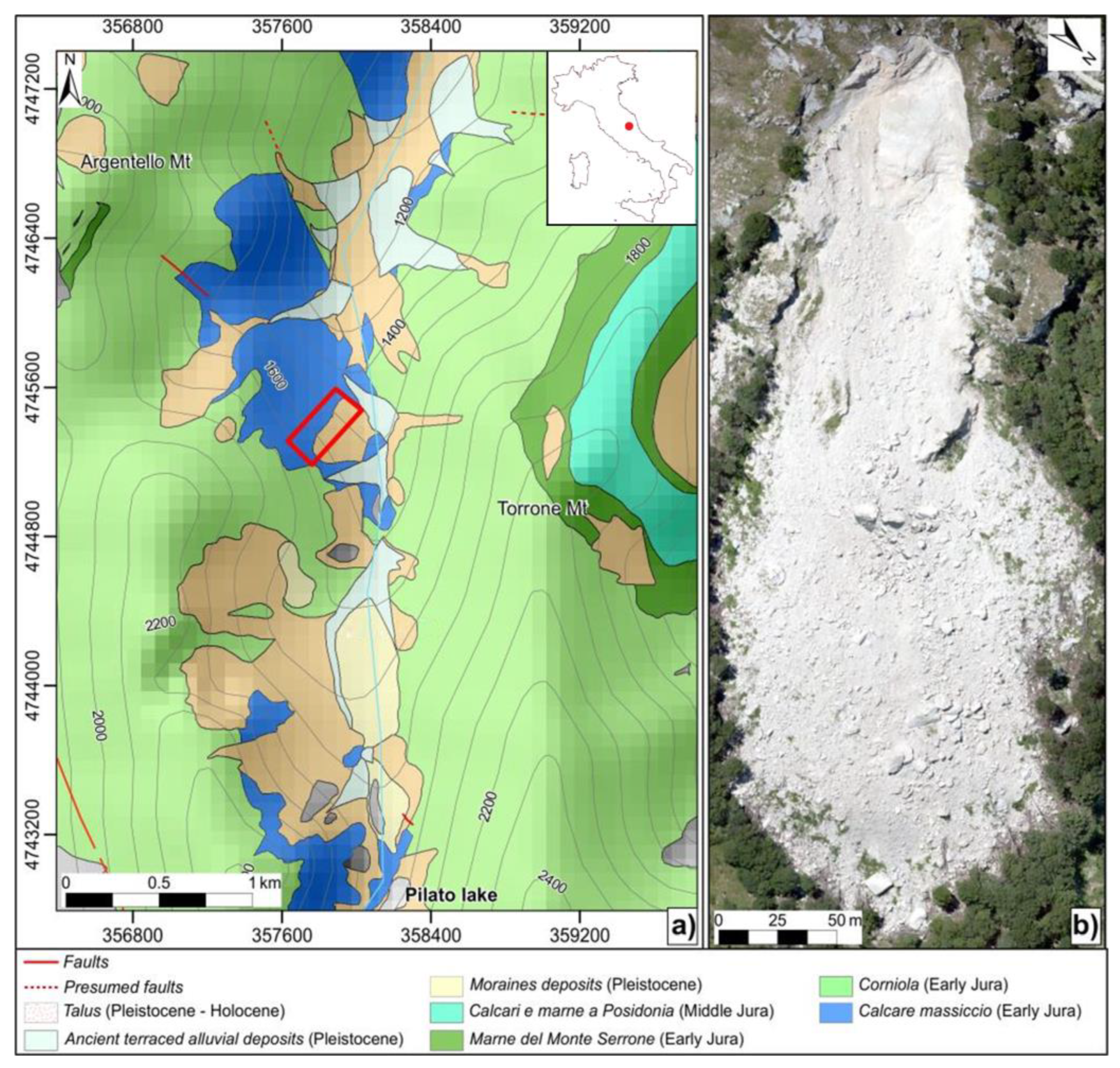
2. Geological and Seismological Setting of the Study Area

The geological setting of the Central Apennines is characterised by a Jurassic to Miocene stratigraphic sequence ([30] and references therein). It experienced multi-phase contractional and extensional deformations stages, with pre-orogenic extension phases followed by the main compressive stage (compressive direction: NE–SW) and a Quaternary extension phase.
The outcropping succession of the study area (Figure 1a) is characterised by massive or coarsely bedded Early Jurassic limestones (Calcare Massiccio Fm.), overlain by several Jurassic marly calcareous units (including Corniola Fm., Marne del Monte Serrone Fm., and Calcari e Marne a Posidonia Fm.). They are then covered by Pleistocene and Holocene deposits of glacial and fluvial origin.
Over the last 2000 years, the study area has been affected by several EQTLs (see the CPTI15 4.0 catalogue, [31]). In fact, after the 1997 Colfiorito–Sellano seismic sequence, a reliable dataset of earthquake-induced landslides was collected, and about 90% of the 250 documented landslides were rockfalls, topples, and rockslides [32,33,34]. As regards the 2016–2017 Central Italy seismic sequence, a total of 1370 landslides were collected. In particular, 170 were triggered by the Accumoli shock (24 August 2016, Mw 6.0), 400 by the Visso shock (26 October 2016, Mw 5.9), and 800 by the Norcia shock (30 October 2016, Mw 6.5).
The Foce rockslide was triggered by the Norcia shock, the epicentre of which was located about 12 km from the landslide. The failure, which involved a rock slope consisting of Calcare Massiccio fm. limestones, occurred along a major N–S normal fault (average dip 50°) at an average elevation of about 1700 m a.s.l. It had a total runout of 370 m, while the crown scarp showed a maximum width of about 60 m (Figure 1b).

3. Materials and Methods

The investigations consisted of geological, structural, geomechanical, and UAV photogrammetric surveys from which the VOM and the orthophotos were generated (Figure 2). To identify the discontinuity systems at the outcrop scale, a VOM of the investigated slope was first developed through structure-from-motion (SfM) photogrammetry based on UAV acquisitions. The discontinuities identified on the VOM were then represented on stereoplots and subdivided into sets.
To evaluate the possible relationships between the joints forming the Foce sliding scar and the regional tectonic setting, the results of the analysis of the rock mass structure at the rockslide outcrop were compared with the distribution of the major discontinuities within an area of about 10 km2. These were both extracted from the official geological maps and inferred from the morphological features identified on aerial photographs (including escarpments, subsequent valleys, ridges, and anomalies of the hydrographic network).
The VOM allowed the reconstruction of the geometry of the complex sliding scar, which was a combination of different major discontinuities. Digitisation of their surfaces provided geomechanical parameters, which were combined with data obtained from traditional geomechanical investigations to evaluate the shear strength parameters for the back analysis of the rockslide. This was conducted with an LE procedure in three dimensions both in static and earthquake loading conditions.

3.1. Remote Sensing Investigations

The VOM of the rockslide scar was reconstructed based on high-resolution images acquired by means of a DJI Mavic 2 Pro UAV and a Yuneec H520E RTK UAV, both equipped with a 1″ CMOS sensor and a 20 MP camera having a focal length of 3.6 mm. The images, acquired with an overlap of 70% in both horizontal and vertical directions, were georeferenced and processed by means of SfM computer vision techniques. This step allowed the completion of the dense point cloud and the construction of different 3D models, including the Digital Elevation Model (DEM) and the orthorectified aerial images of the rockslide. The structural features on the 3D model were then analysed with OpenPlot (Figure 3a,b) and CloudCompare v2.10.2 (Figure 3c) software.
OpenPlot was used to extract the discontinuity planes from their traces previously defined over the virtual outcrop. The software computes the best-fit plane between the digitised polyline and the outcrop topography [35] and displays the obtained plane on the point cloud. Each discontinuity is defined by several parameters, including coordinates and orientation (dip and dip direction). Orientation data were then clustered, and the various joint sets were defined.
CloudCompare was used to perform a comparative analysis, based on a data refinement (i.e., adjustment of the point clouds, remotion of the ‘floating’ points, and resizing of the ‘floating’ points with respect to the rockslide scar), with the aim of extracting the major surfaces of the landslide scar through the plugin ‘Facets’, as described in [36]. The plugin divides the point cloud into clusters of points sharing user-defined parameters of coplanarity and extracts planar features (polygons) from the 3D point cloud. Each planar facet is adjusted to fit the original point cloud, and it is defined as a mesh surface with contour, extent, centroid, and normal values. The dip and dip direction of each determined facet allowed the classification of the main rockslide scar surfaces into sets, represented in a stereoplot diagram. The Fast Marching (FM) least square fitting method [37] was selected with the following user-defined parameters: (i) Octree level, (ii) Max distance at n%, (iii) Min points per facet, and (iv) Max edge length. The octree level defines the size of the smallest box in the space partitioning and, therefore, the grid resolution. The other three parameters calibrate the geometries of the facets. The max distance at n% determines that a certain percentage of points must be closer to each other than the specified value to be part of the same facet. The min points per facet filters the facets smaller than the specified value, and the max edge length defines the maximum length of the facets’ contour.
Finally, the sets of discontinuities obtained from the trace digitisation (Open Plot) and from the analysis of the slide scar surfaces (CloudCompare) were compared.

3.2. Geomechanical Investigations

The strength of the discontinuity surfaces was measured through in situ Schmidt hammer tests, while the roughness was estimated at a small scale from 100 mm long profiles measured on rock block faces with a mechanical profilometer and at a large scale from 10 m long profiles extracted from the 3D point cloud model. The roughness determination through conventional methods or photogrammetry surveys has been broadly discussed in the literature (see, e.g., [38] and references therein). Since the flights were performed at a height of about 80 m, the Ground Sampling Distance (GSD) was about 20 mm. This resolution, deriving from photographs with resolutions ranging from 20 to 30 mm per pixel, was sufficiently high to ensure the accuracy of the roughness information, allowing the detection of the medium- to large-scale undulation angles of the sliding surface.
The characterisation of the intact rock was also conducted on specimens of the Calcare Massiccio Fm. through laboratory tests, i.e., uniaxial and compression, indirect tensile, and ultrasonic pulse tests.

3.3. Numerical Modelling

Once the geological–geotechnical model of the slope was reconstructed, a series of slope stability analyses was performed using Plaxis 3D LE [39]. To reconstruct the pre-failure topographic surface (Figure 4a), the post-event contour lines were manually adjusted, based on the interpretation of a pre-event, 20 m DEM (freely available at https://www.regione.marche.it/Regione-Utile/Ambiente/Cartografia-e-informazioni-territoriali/Repertorio#DTM accessed on 12 September 2023) and stereo pairs of aerial photographs acquired in 1990 (provided by the Umbria Region). The main surfaces forming the rockslide scar, which were identified after the structural analysis (see Section 4.1), were also considered in the geotechnical model of the slope. In this respect, the actual slip surface (Ss) was imported into the code from the post-event DEM and thoroughly cut within the wedge scar area (Figure 4b). Two types of slope stability analyses have been carried out: static analyses and dynamic analyses accounting for different earthquake inputs.

4. Results

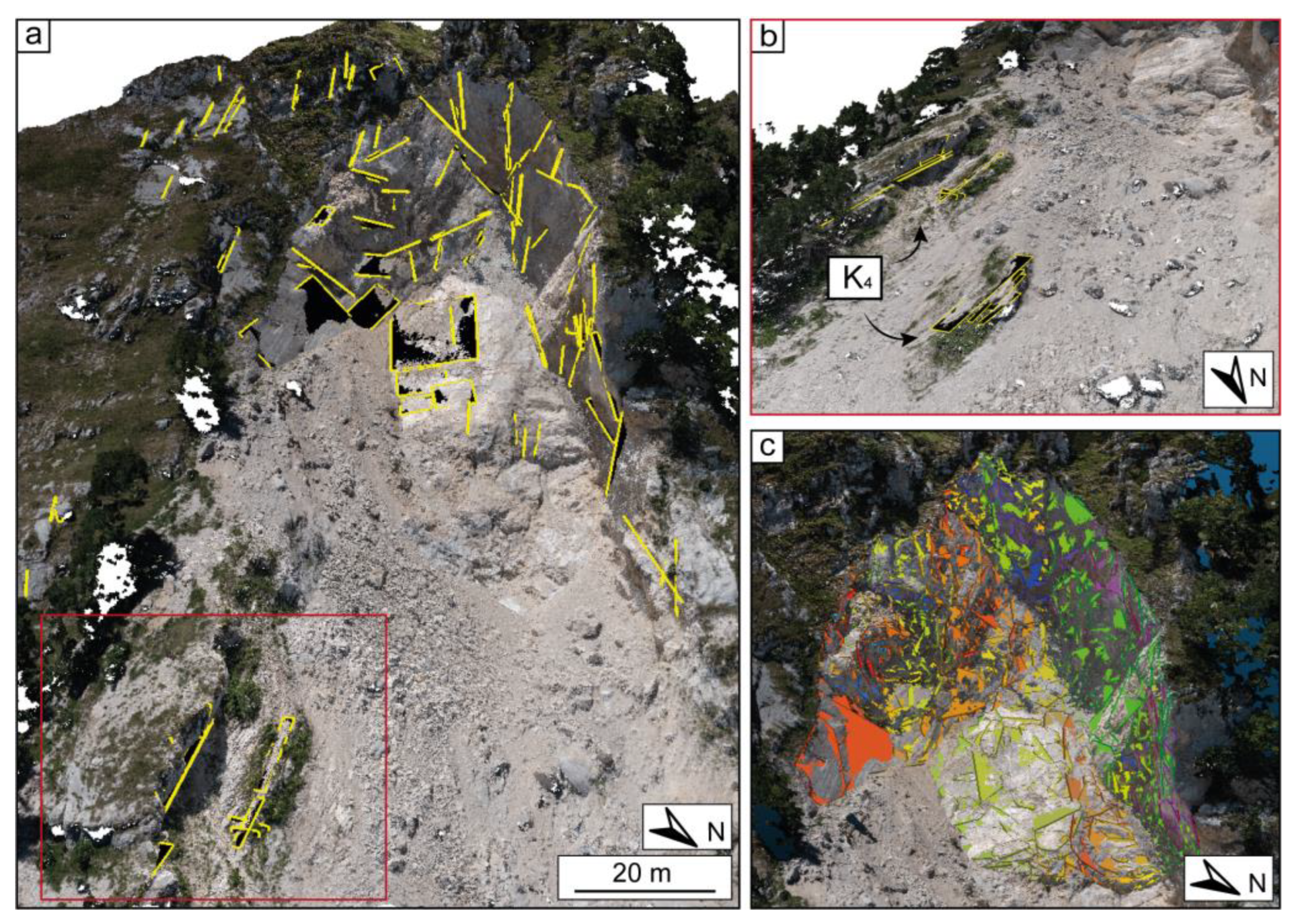
4.1. Structural Analysis

To define the main discontinuity sets affecting the rock mass, a total of 105 discontinuities were digitised from the VOM (Open Plot analysis) and clustered through stereonet projections, together with the data collected through the morphostructural analysis. Four main sets were identified (Table 1), striking NW–SE (K1), NE–SW (K2), N–S (K3), and NNW–SSE (K4).
The orientations of the main discontinuity surfaces that form the rockslide scar were obtained through the CloudCompare ‘Facets’ plugin (Figure 5). On the digital model of the scar, 766 facets were identified. The Max distance value was manually determined to accurately fit the point cloud. About 15 regular planes were identified within the point cloud as ‘reference planes’, and for each of them a best-fitting plane was computed, creating a meshed surface. Subsequently, the cloud-to-mesh distance was calculated and shown in histograms. The average distance value for the analysed planes represented the Max distance used for the final model. The remaining parameters of the final model were determined with a trial-and-error approach to obtain input parameters that yield the best fit for the original point cloud (Table 2).
In the resulting, simplified model, the scar is composed of four major surfaces (Table 1), striking NW–SE (038°/64°, S1), NE–SW (122°/81°, S2), N–S (089°/79°, S3), and NNW–SSE (069°/44°, Ss). The detached wedge was considered as the intersection of the four detected surfaces: the main sliding surface (Ss), the right-lateral and left-lateral surfaces, S1 and S2 respectively, and a back surface (S3, Figure 5). The Ss has a length of about 115 m, while the S1 and S2 surfaces show a maximum height of about 8 m and 19 m, respectively. The mass movement involved an estimated volume of about 40,000 m3. The geometry and volume of the rockslide were estimated from the VOM by measuring the dimensions of the four defined surfaces and by reconstructing the pre-failure slope geometry.

4.2. Stability Analyses

4.2.1. Preliminary Kinematic Analyses

A preliminary kinematic analysis was conducted using DIPS software [40] under the hypothesis of a wedge delimited by two discontinuity surfaces assuming an average orientation of the slope face of 064°/46°. It is important to specify that the dip value was estimated from the reconstructed, pre-failure DEM (Figure 4a).
The results of the graphic procedures indicate that the planar sliding on the Ss discontinuity is the prevalent failure mechanism (Figure 6). Furthermore, sliding along the planes Ss and S3 is not kinematically possible, whilst sliding along the Ss and S2 planes is kinematically possible, but the resulting wedge is very narrow. Finally, sliding along the Ss and S1 planes is virtually possible given that the dispersion of the results could move the pole of the intersection line of the two planes outwards. The analysis was computed considering lateral limits of 30° and a friction angle for the discontinuity planes equal to 40°, as reported in a preceding study focused on the same rock type [17].

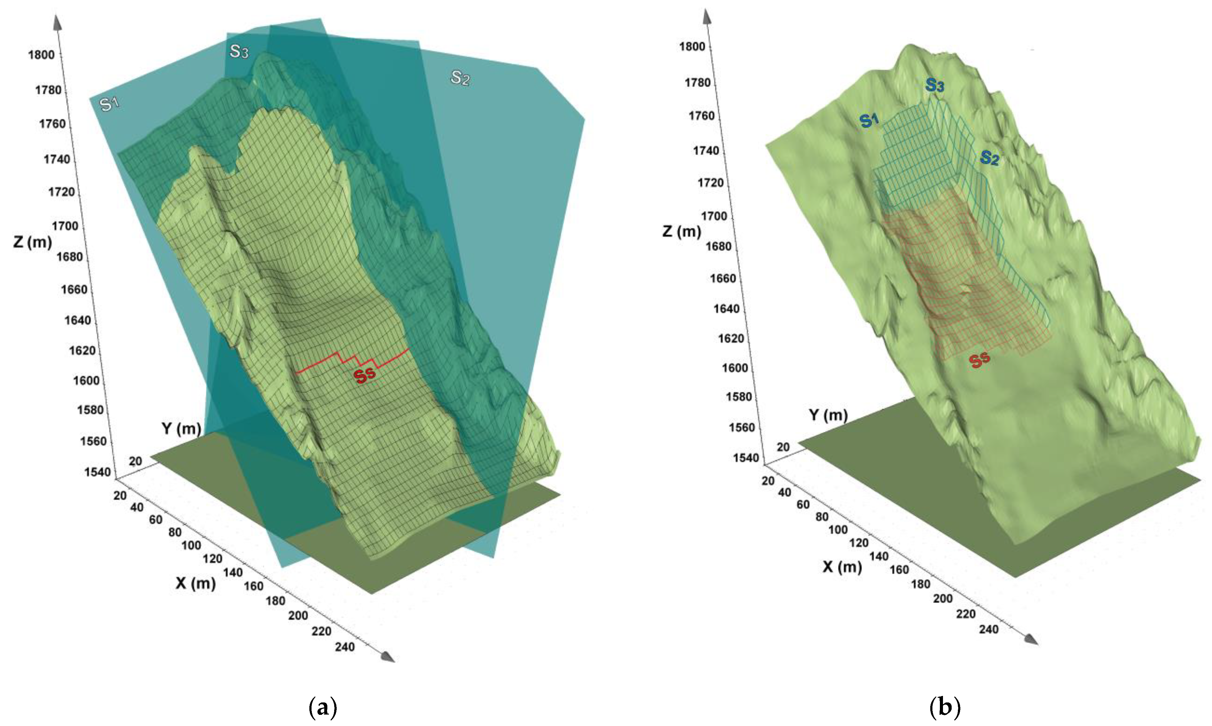
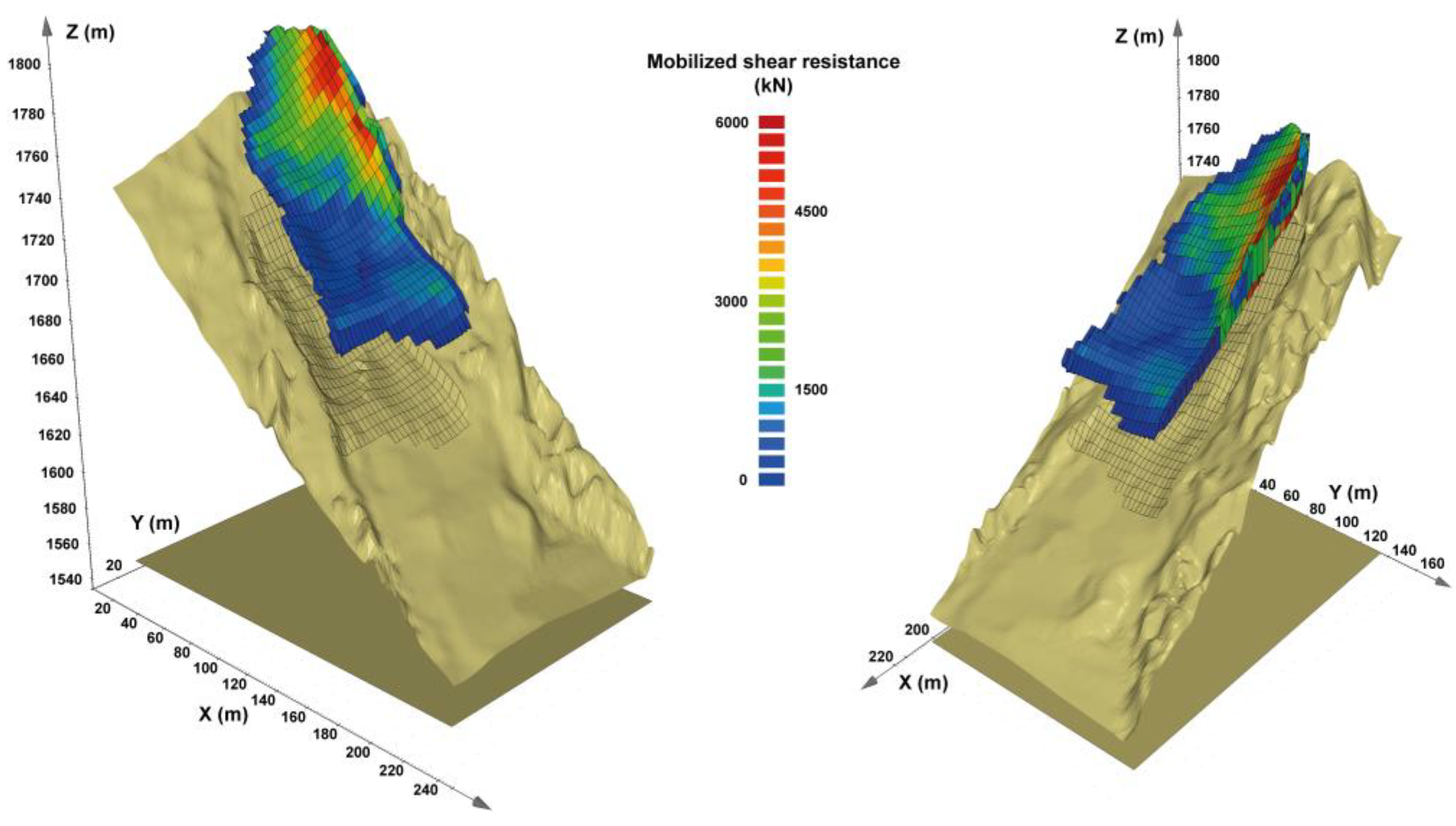
4.2.2. Three-Dimensional Limit Equilibrium Analyses

The rockslide body was modelled as a fractured rock mass delimited at the top by the slope surface and at its bottom by a composite sliding surface formed by the different discontinuities identified in the structural analysis. We opted for the use of the LE Sarma method [41] because it is suited for relatively simple and homogeneous landslides bodies where an internal rupture is hypothesised. In fact, on one hand, the slide mass is formed by a single rock type; on the other, the significant fragmentation experienced by a rock mass having few, persistent discontinuities suggests an internal rupture at incipient sliding. Furthermore, the Sarma formulation is conceived for pseudo-static seismic analyses [42] and can be applied to any shape of sliding surfaces [43,44,45], satisfying both force and moment equilibrium conditions. In this respect, it is important to specify that, in its 3D extension, the method can solve force and moment equilibrium equations in two orthogonal directions (i.e., sliding and transverse directions) through the approach proposed by [46], allowing a more consistent FS evaluation for asymmetric geometries (as in the case of the Foce rockslide). The discontinuities forming the slide surface were assigned the shear strength parameters based on the geomechanical characterization illustrated above.
If we exclude the discontinuities forming the composite sliding surface, no other specific major discontinuity cutting the inner part of the rockslide body before failure could be identified at this stage of the study. Thus, the shear strength at the boundaries of each slice forming the rockslide body was assimilated to that of a homogeneously fractured rock mass, expressed by the generalised Hoek–Brown empirical criterion in the form [47]:
σ 1 = σ 3 + σ c i m b σ 3 σ c i + s b a
where:
-
σci is the uniaxial compressive strength of the rock material;
-
mb expresses the effect of the confining stress and it is equal to the coefficient mi of the rock material, scaled to the rock mass;
-
sb expresses the intensity of the damage (fracturing) of the rock mass;
-
a adjusts the curvature for the application to the rock mass.
We decided to use the Hoek–Brown criterion as it describes the shear strength of a fractured rock mass without preferential weak discontinuity sets [48,49]. Its non-linear formulation can also account for the sharp strength variation at low confining stresses. All rock mass-related parameters, whose expressions are reported in [47], depend on the rock mass structure that is expressed by the Geological Strength Index (GSI); mb and sb are also influenced by the degree of loosening, expressed by the disturbance factor (D) of the rock mass.
In the analyses, the D was assumed equal to unity due to the severe stress release experienced by the slope over a very long period of time, while the GSI varies in the range 65–75. The average value of 70 was initially assumed in the analyses (Table 3). This range accounts for the relatively good quality of the rock mass, characterised by a blocky structure and large spacing of the bedding joints (i.e., about 5 m). The mi value was chosen according to typical values reported in the literature for micritic limestones [50]. The shear strength of the rock discontinuities controlling failure was modelled according to a modified expression of the Barton–Bandis criterion, which accounts for scale effects at the block scale and for large-scale undulations [51]:
τ = σn tan [JRCn log10 (JCSn/σn) + φr + ω]
where τ is the shear strength; σn is the normal stress acting on the discontinuity surface; φr is the residual friction angle, which was assumed equal to 31° [17]; and ω is the inclination of large-scale undulations along the sliding direction, measured on roughness profiles from the point cloud. JCSn and JRCn are the scale-corrected Joint Compressive Strength and Joint Roughness Coefficient, respectively [52]:
JCSn = JCS0 (Ln/L0)−0.03 JRC0
JRCn = JRC0 (Ln/L0)−0.02 JRC0
where JCS0 and JRC0 are values estimated from small-scale field measurements; L0 is the length of the reference profiles (100 mm); and Ln is the block scale discontinuity length, which is assumed to be equal to the average spacing of bedding joints [17]. JCS0 was estimated from the rebound height, RL, corrected for the actual hammer inclination, through the empirical correlation:
JCS0 = 2.63 e0.061 RL
which was obtained by fitting many pairs of UCS and RL values measured on NX cylindrical specimens from different carbonate lithotypes of the Umbria–Marche sequence [17].
The FS provided by the analyses (1.13) suggests that the slope was characterised by stability conditions not far from the limit equilibrium before the earthquake. Nevertheless, an analysis disregarding large-scale discontinuity undulations yields an FS value lower than unity (0.93), thus suggesting that the waviness of major joints can play a crucial role in this context [53].
Dynamic analyses were conducted with the approach proposed by [54], based on coseismic displacement. We applied the seismic input recorded at the ‘Arquata del Tronto’ accelerometric station during the 30 October 2016 Norcia earthquake, i.e., the one that likely triggered the rockslide. The accelerometric recording was extracted from the ITACA database—ITalian ACcelerometric Archive (https://itaca.mi.ingv.it/ItacaNet_40/#/home accessed on 12 September 2023).
This station, built on bedrock on top of a morphologic ridge consisting of carbonate rocks, is located at 15.6 km from the epicentre of the Norcia earthquake (the epicentral distance of the Foce rockslide is 12.5 km). The applied signal has three features that make it suitable as the seismic input for analysing the Foce rockslide, specifically: (i) it includes a realistic seismic wave attenuation (the comparable epicentral distance of the slide and the accelerometric station), (ii) it is not affected by modifications induced by possible soil layers below the station, and (iii) it includes a topographic effect comparable to that expected at the Foce rock slope. We considered the E–W component since the rockslide is roughly E–W oriented.
The obtained displacement (28 cm) is consistent with that necessary to largely overcome the peak strength of discontinuities [55] and the critical threshold (5 cm) proposed in the literature ([56] and references therein).

5. Discussions

In the above-described analyses, we showed how the UAV-based approach and the digital data collection were fundamental, since the area is currently inaccessible for direct field measurements due to the steep slopes.
The analysis performed with OpenPlot indicated that the study area is characterised by the presence of four main sets of discontinuities, i.e., K1–K4. Similarly, the geometry of the rockslide scar was defined by four main surfaces (S1–S3 and SS), whose orientation follows that of the discontinuity sets (Table 1). Such a scenario suggests that the pre-existing K1, K2, K3, and K4 discontinuity sets played a critical role in the wedge detachment, with the major sliding surface and the lateral surfaces developing along preferential pathways represented by the background discontinuity sets. In particular, the principal sliding surface (Ss) reactivated a low-angle normal fault corresponding to the discontinuity set K4 and widely occurring in the study area (Figure 3b). Moreover, the kinematic analysis performed on the defined sliding surface graphically supported that the planar sliding on the Ss surface was the most likely failure mechanism (Figure 6).
Numerical analyses indicate that the slope was not far from failure even in static conditions, especially when the low roughness values for major discontinuities are considered. However, it is quite evident that the reliability of this result strongly depends on the robustness of the different input parameters. To show their influence on the overall stability of the investigated slope, we performed a sensitivity analysis. The results (Table 4) indicate that the variation of the parameters controlling the strength of the landslide body (i.e., GSI and σci) between minimum and maximum values (obtained from site observations and laboratory tests) causes FS variations of 16.8% and 15% for the GSI and σci, respectively. However, in both cases the FS is always greater than 1. With reference to the discontinuity parameters, we can observe that the JCS has a limited influence on stability conditions. Conversely, the JRC and ω play a significant role, which results not only in a substantial FS variation (from 24.8% to 48.8%) but also in the achievement of failure conditions when minimum values are used.
Such evidence reflects the importance of the roughness features and, in a broader view, of the geostructural setting as a predisposing factor to rockslide triggering, as it was noticed for other rockslides triggered by the 2016–2017 seismic sequence in the same area [23]. However, the attitude of the main discontinuity sets affects not only the potential failure mechanisms (as shown in the kinematic analysis) but also the shear strength of the entire rock mass. Such an influence can be easily estimated in symmetrical conditions, but it can be more complex for non-symmetrical geometries, as in the Foce case. In this respect, the method of analysis used in this work (i.e., 3D analysis considering bidirectional slice interaction) can provide more realistic results, notwithstanding the simplification of the model. Additional static analyses performed disregarding in each simulation the contribution to the shear strength of one of the three main sets of discontinuities show that discontinuity S2 has the largest influence on the slope stability. If its contribution is not considered, the FS decreases by 42.5% (Table 5). S1 has a lesser impact; if it is disregarded, the FS reduces only by 8.8%. The significance of S2 can also be inferred from the geometry of the rockslide body. In this respect, the left side shows a larger thickness (approximately 30 m) of the detached mass, and, in turn, a greater surface extent on which shear strength can be mobilised (Figure 7).
Though we assumed that the Norcia earthquake was the triggering event, it is not possible to exclude a priori the 26 October 2016 Visso earthquake as an alternative triggering event, being characterised by a distance of 15.3 km from the Foce rockslide. Therefore, we performed a further dynamic analysis considering the accelerogram recorded by the Arquata del Tronto station during the event. If we compare this accelerogram with that of 30 October 2016, we can note that the former had significantly lower PGA peaks with the same duration (Figure 8). Despite the signal features indicating that the 26 October event was less severe than the 30 October one, the Newmark analysis shows that it was sufficiently strong to cause a coseismic displacement of 1.5 cm, although lower than the 5 cm critical threshold. In this sense, it is interesting to point out that the maximum PGA values recorded for both earthquakes are three to six times higher than those estimated through a ground motion prediction equation (GMPE) to account for seismic wave attenuation [57] (Figure 9). Since stratigraphic amplification phenomena can be excluded for the study area (see Section 4.2), the difference between the estimated and recorded PGA values can be explained by the topographic amplification effects related to the steepness of the investigated slope, which are implicitly accounted for by the selected recording. An insight into these effects, which have been highlighted for other rockslide phenomena that occurred during the 2016 earthquake [23], would require more advanced numerical analyses, which are beyond the scope of this work, which focused on a simplified approach for the study of EQTLs. However, the performed activities provided not only useful, quantitative data on a recurrent type of earthquake-induced failure on mountain slopes but also a relatively simple approach, largely based on UAV-derived data, that can be applied to other case studies: (i) in order to ascertain if more advanced and time-consuming analyses add significant improvements in the evaluation of the stability of a rock slope in seismic conditions; and (ii) in order to prioritise, in similar geological and geostructural contexts, the level of detail and accuracy of the analyses to be carried out.

6. Conclusions

In this study, the earthquake-induced Foce rockslide was analysed through using input data obtained with a UAV-based approach. The geometric and kinematic reconstruction was conducted by combining the structural analysis of the study area with remote digitisation of the discontinuities from a VOM, geomechanical investigation of the intact rock, and numerical simulations of slope stability. The main findings can be summarised as follows:
-
The study area is characterised by the occurrence of four main sets of discontinuities, striking NW–SE, NE–SW, NNW–SSE, and N–S.
-
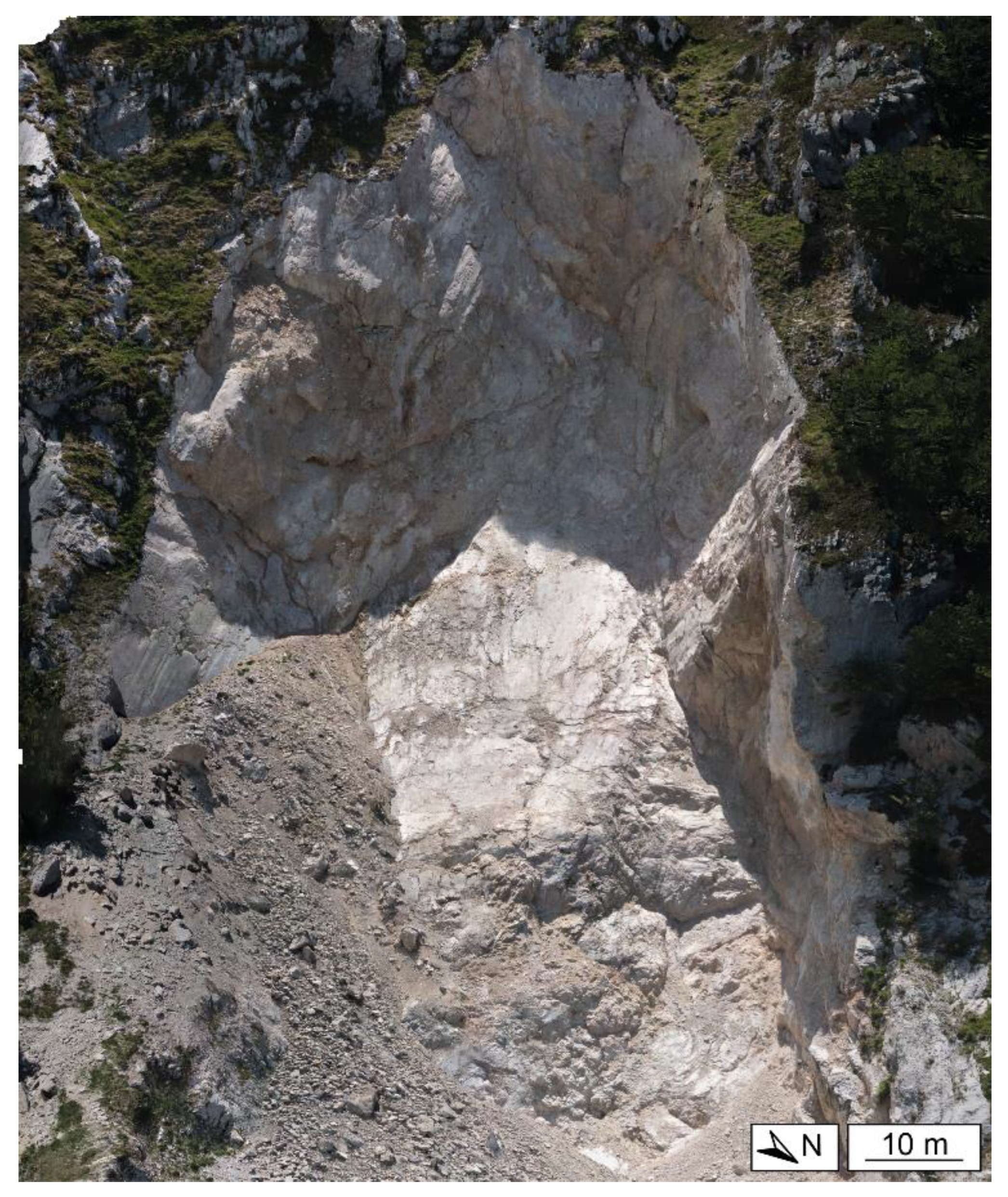
The principal sliding surface and the lateral surfaces of the rockslide scar reactivated the pathways of pre-existing NW–SE and NE–SW trending sets. In particular, the kinematic analysis showed that the failure mechanism that occurred was the planar sliding on the main sliding surface (Ss), which corresponds to the set K4.
-
The slope stability analyses under static conditions highlighted how the slope was already not far from a critical status even before the earthquake, mainly due to the geostructural and geomechanical settings. Regarding the latter aspect, the key role played by the joint roughness was also pointed out.
-
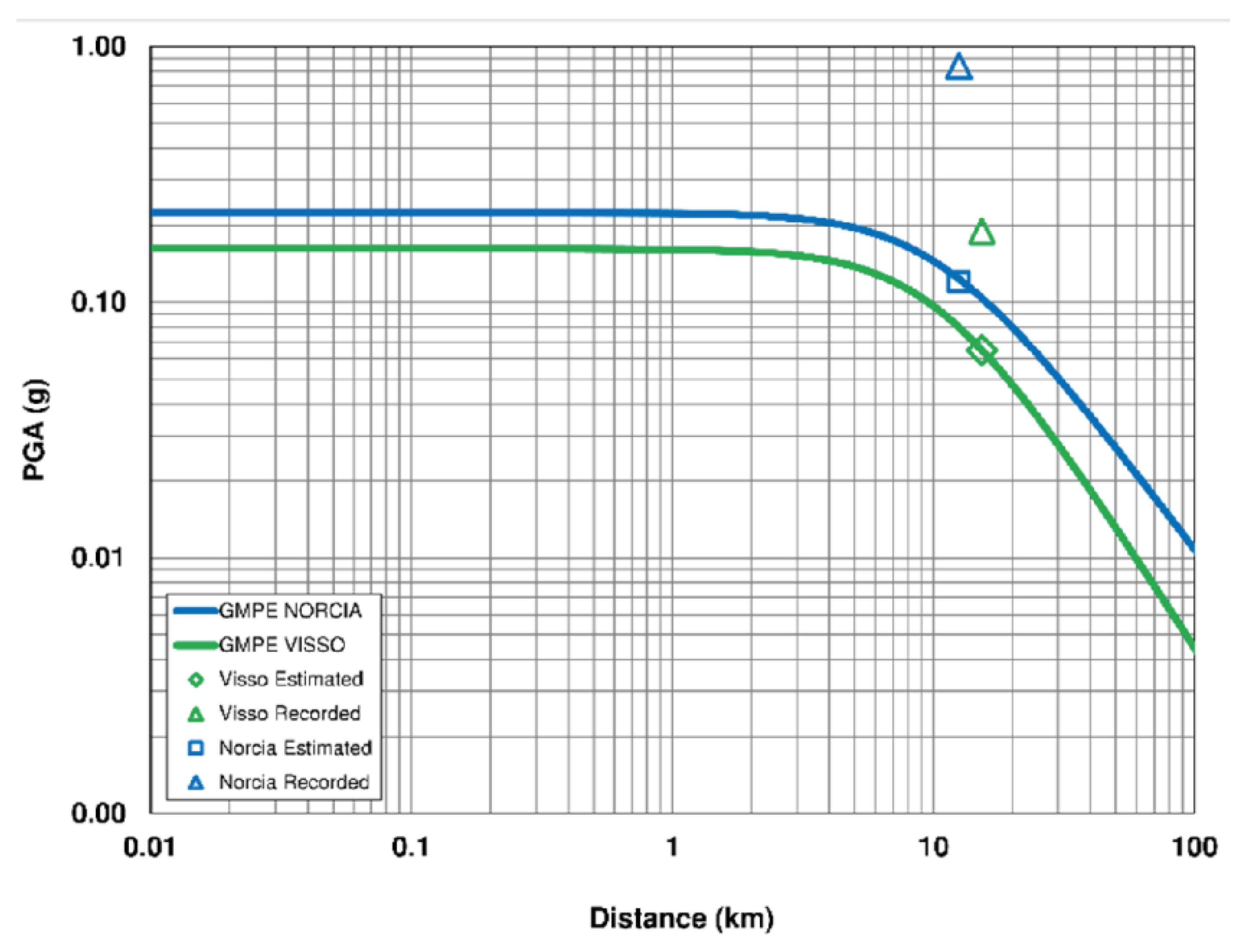
The analyses in dynamic conditions provided reliable results both in terms of coseismic displacements (28 cm) and mobilised volume (40,000 m3). Such analyses confirm that the Norcia earthquake was the triggering event, although, in principle, the Visso earthquake could also have caused coseismic displacements.
Despite the unavoidable uncertainties mostly related to the simplification of the model, the results obtained with the proposed approach are consistent with the real landslide event and confirm how UAV photogrammetric surveys can represent a valuable technique for supporting similar analyses. Regarding the case of the Foce rockslide, in the light of the potential, topographic amplification effects mentioned in the Discussions section, future analyses in this area will undertake a better evaluation of this phenomenon through more advanced numerical analyses, with the aim of defining its role in the triggering process. In a broader perspective, the proposed approach can be applied to other rockslide events where the geostructural setting plays a key role in slope stability. In this sense, the rationale could be to obtain an initial, overall evaluation of the failure conditions and then to establish more in-depth analyses, if necessary.

Author Contributions

Conceptualization, A.S. and P.T.; methodology, L.S., L.M. and G.F.; software, L.S. and L.M.; validation, G.F. and P.T.; investigation, L.S., G.F. and P.T.; resources, A.S. and P.T.; writing—original draft preparation, L.S. and L.M.; writing—review and editing, L.S., L.M., G.F. and P.T.; visualization, L.S. and L.M.; supervision, A.S.; funding acquisition, A.S. and P.T. All authors have read and agreed to the published version of the manuscript.

Funding

The research was partially funded by the Italian Civil Protection Department RELUIS project (2018), PR8-UR18-WP2 UNINA (P.I. A. Santo). P. Tommasi and L. Schilirò benefitted from the EmerTer Project, funded by Italian D.P.C. (Principal Investigator M. Moscatelli); the FraSi Project, funded by Italian Ministry for the Environment and Protection of Land and Sea (Principal Investigator P. Reichenbach); the Sapienza University project, “Failures occurred during the 2016–2017 Central Italy seismic sequence based on site investigation and numerical modelling: hints for hazard mitigation in high seismicity areas” (P.I. Giuseppe Lanzo); and the CNR-IGAG Project “Stabilità dei Versanti in Condizioni statiche e dinamiche” (P.I. Paolo Tommasi).

Data Availability Statement

The data presented in this study are available on request from the corresponding author.

Acknowledgements

The authors thank Melania De Falco and Ermanno Marino for the help in preparing the geological maps and for contributing to drone surveys, respectively. The authors also wish to thank Luca Verrucci for his contribution during the geomechanical surveys. The authors greatly appreciated the cooperation of the Parco Nazionale dei Monti Sibillini (namely A. Rossetti and M. Piccini) for the authorization for scientific activities within the National Park. Pre-failure aerial photo stereopairs and 20-m DTM were kindly provided by Umbria Region (Sistema Cartografico Regionale) and Marche Region (Sistema Cartografico Regionale e Informativo Territoriale), respectively.

Conflicts of Interest

The authors declare no conflicts of interest.

References

  1. Carlton, B.; Kaynia, A.M.; Nadim, F. Some important considerations in analysis of earthquake-induced landslides. Geoenviron. Disasters 2016, 3, 11. [Google Scholar] [CrossRef]
  2. Basharat, M.; Riaz, M.T.; Jan, M.Q.; Xu, C.; Riaz, S. A review of landslides related to the 2005 Kashmir Earthquake: Implication and future challenges. Nat. Hazards 2021, 108, 1–30. [Google Scholar] [CrossRef]
  3. Song, C.; Yu, C.; Li, Z.; Utili, S.; Frattini, P.; Crosta, G.; Peng, J. Triggering and recovery of earthquake accelerated landslides in Central Italy revealed by satellite radar observations. Nat. Commun. 2022, 13, 7278. [Google Scholar] [CrossRef] [PubMed]
  4. Chigira, M.; Wu, X.; Inokuchi, T.; Wang, G. Landslides induced by the 2008 Wenchuan earthquake, Sichuan, China. Geomorphology 2010, 118, 225–238. [Google Scholar] [CrossRef]
  5. Fan, X.; Yunus, A.P.; Scaringi, G.; Catani, F.; Siva Subramanian, S.; Xu, Q.; Huang, R. Rapidly Evolving controls of landslides after a strong earthquake and implications for hazard assessments. Geophys. Res. Lett. 2021, 48, e2020GL090509. [Google Scholar] [CrossRef]
  6. Fan, X.; Xu, Q.; van Westen, C.J.; Huang, R.; Tang, R. Characteristics and classification of landslide dams associated with the 2008 Wenchuan earthquake. Geoenviron. Disasters 2017, 4, 12. [Google Scholar] [CrossRef]
  7. Ehteshami-Moinabadi, M.; Nasiri, S. Geometrical and structural setting of landslide dams of the Central Alborz: A link between earthquakes and landslide damming. Bull. Eng. Geol. Environ. 2019, 78, 69–88. [Google Scholar] [CrossRef]
  8. Chen, T.C.; Lin, M.L.; Wang, K.L. Landslide seismic signal recognition and mobility for an earthquake-induced rockslide in Tsaoling, Taiwan. Eng. Geol. 2014, 171, 31–44. [Google Scholar] [CrossRef]
  9. Luo, J.; Pei, X.; Evans, S.G.; Huang, R. Mechanics of the earthquake-induced Hongshiyan landslide in the 2014 Mw 6.2 Ludian earthquake, Yunnan, China. Eng. Geol. 2019, 251, 197–213. [Google Scholar] [CrossRef]
  10. Oswald, P.; Strasser, M.; Hammerl, C.; Moernaut, J. Seismic control of large prehistoric rockslides in the Eastern Alps. Nat. Commun. 2021, 12, 1059. [Google Scholar] [CrossRef]
  11. Strom, A.; Wang, G. Some Earthquake-Induced Rockslides in the Central Asia Region. In Coseismic Landslides: Phenomena, Long-Term Effects and Mitigation; Towhata, I., Wang, G., Xu, Q., Massey, C., Eds.; Springer Nature: Singapore, 2022; pp. 143–168. [Google Scholar]
  12. Antonielli, B.; Della Seta, M.; Esposito, C.; Scarascia Mugnozza, G.; Schilirò, L.; Spadi, M.; Tallini, M. Quaternary rock avalanches in the Apennines: New data and interpretation of the huge clastic deposit of the L’Aquila Basin (central Italy). Geomorphology 2020, 361, 107194. [Google Scholar] [CrossRef]
  13. Putignano, M.L.; Di Luzio, E.; Schilirò, L.; Pietrosante, A.; Giano, S.I. The Pretare-Piedilama clastic deposit: New evidence of a Quaternary rock avalanche event in central Apennines (Italy). Water 2023, 15, 753. [Google Scholar] [CrossRef]
  14. Franke, K.W.; Lingwall, B.N.; Zimmaro, P.; Kayen, R.E.; Tommasi, P.; Chiabrando, F.; Santo, A. Phased reconnaissance approach to documenting landslides following the 2016 Central Italy earthquakes. Earthq. Spectra 2018, 34, 1693–1719. [Google Scholar] [CrossRef]
  15. Martino, S.; Bozzano, F.; Caporossi, P.; D’Angiò, D.; Della Seta, M.; Esposito, C.; Fantini, A.; Fiorucci, M.; Giannini, L.M.; Iannucci, R.; et al. Impact of landslides on transportation routes during the 2016–2017 Central Italy seismic sequence. Landslides 2019, 16, 1221–1241. [Google Scholar] [CrossRef]
  16. Romeo, S.; Di Matteo, L.; Melelli, L.; Cencetti, C.; Dragoni, W.; Fredduzzi, A. Seismic-induced rockfalls and landslide dam following the October 30, 2016 earthquake in Central Italy. Landslides 2017, 14, 1457–1465. [Google Scholar] [CrossRef]
  17. Forte, G.; Verrucci, L.; Di Giulio, A.; De Falco, M.; Tommasi, P.; Lanzo, G.; Franke, K.W.; Santo, A. Analysis of major rock slides that occurred during the 2016–2017 Central Italy seismic sequence. Eng. Geol. 2021, 290, 106194. [Google Scholar] [CrossRef]
  18. Schilirò, L.; Rossi, M.; Polpetta, F.; Fiorucci, F.; Fortunato, C.; Reichenbach, P. A web-based GIS (web-GIS) database of the scientific articles on earthquake-triggered landslides. Nat. Hazards Earth Syst. Sci. 2023, 23, 1789–1804. [Google Scholar] [CrossRef]
  19. Valkaniotis, S.; Papathanassiou, G.; Ganas, A. Mapping an earthquake-induced landslide based on UAV imagery; case study of the 2015 Okeanos landslide, Lefkada, Greece. Eng. Geol. 2018, 245, 141–152. [Google Scholar] [CrossRef]
  20. Ma, S.; Wei, J.; Xu, C.; Shao, X.; Xu, S.; Chai, S.; Cui, Y. UAV survey and numerical modeling of loess landslides: An example from Zaoling, southern Shanxi Province, China. Nat. Hazards 2020, 104, 1125–1140. [Google Scholar] [CrossRef]
  21. Baghbanan, A.; Kefayati, S.; Torkan, M.; Hashemolhosseini, H.; Narimani, R. Numerical probabilistic analysis for slope stability in fractured rock masses using DFN-DEM approach. Int. J. Min. Geo-Eng. 2017, 51, 79–90. [Google Scholar] [CrossRef]
  22. Cheng, Z.; Gong, W.; Tang, H.; Juang, C.H.; Deng, Q.; Chen, J.; Ye, X. UAV photogrammetry-based remote sensing and preliminary assessment of the behavior of a landslide in Guizhou, China. Eng. Geol. 2021, 289, 106172. [Google Scholar] [CrossRef]
  23. Verrucci, L.; Forte, G.; De Falco, M.; Tommasi, P.; Lanzo, G.; Franke, K.W.; Santo, A. Instantaneous limit equilibrium back analyses of major rockslides triggered during the 2016–2017 central Italy seismic sequence. Nat. Hazards Earth Syst. Sci. 2023, 23, 1177–1190. [Google Scholar] [CrossRef]
  24. Piras, M.; Taddia, G.; Forno, M.G.; Gattiglio, M.; Aicardi, I.; Dabove, P.; Russo, S.L.; Lingua, A. Detailed geological mapping in mountain areas using an unmanned aerial vehicle: Application to the Rodoretto Valley, NW Italian Alps. Geomat. Nat. Hazards Risk 2017, 8, 137–149. [Google Scholar] [CrossRef]
  25. Francioni, M.; Antonaci, F.; Sciarra, N.; Robiati, C.; Coggan, J.; Stead, D.; Calamita, F. Application of Unmanned Aerial Vehicle Data and Discrete Fracture Network Models for Improved Rockfall Simulations. Remote Sens. 2020, 12, 2053. [Google Scholar] [CrossRef]
  26. Massaro, L.; Corradetti, A.; Vinci, F.; Tavani, S.; Iannace, A.; Parente, M.; Mazzoli, S. Multiscale fracture analysis in a reservoir-scale carbonate platform exposure (Sorrento Peninsula, Italy): Implications for fluid flow. Geofluids 2018, 2018, 1–10. [Google Scholar] [CrossRef]
  27. Schilirò, L.; Robiati, C.; Smeraglia, L.; Vinci, F.; Iannace, A.; Parente, M.; Tavani, S. An integrated approach for the reconstruction of rockfall scenarios from UAV and satellite-based data in the Sorrento Peninsula (southern Italy). Eng. Geol. 2022, 308, 106795. [Google Scholar] [CrossRef]
  28. Fazio, N.L.; Perrotti, M.; Andriani, G.F.; Mancini, F.; Rossi, P.; Castagnetti, C.; Lollino, P. A new methodological approach to assess the stability of discontinuous rocky cliffs using in-situ surveys supported by UAV-based techniques and 3-D finite element model: A case study. Eng. Geol. 2019, 260, 105205. [Google Scholar] [CrossRef]
  29. Hungr, O.; Leroueil, S.; Picarelli, L. The Varnes classification of landslide types, an update. Landslides 2014, 11, 167–194. [Google Scholar] [CrossRef]
  30. Pierantoni, P.; Deiana, G.; Galdenzi, S. Stratigraphic and structural features of the sibillini mountains(Umbria- Marche Apennines, Italy). Ital. J. Geosci. 2013, 132, 497–520. [Google Scholar] [CrossRef]
  31. Rovida, A.; Locati, M.; Camassi, R.; Lolli, B.; Gasperini, P.; Antonucci, A. Catalogo Parametrico dei Terremoti Italiani (CPTI15), Versione 4.0; Instituto Nazionale di Geofisica e Vulcanologia (INGV): Roma, Italy, 2022. [Google Scholar] [CrossRef]
  32. Esposito, E.; Porfido, S.; Simonelli, A.L.; Mastrolorenzo, G.; Iaccarino, G. Landslides and other surface effects induced by the 1997 Umbria–Marche seismic sequence. Eng. Geol. 2000, 58, 353–376. [Google Scholar] [CrossRef]
  33. Guzzetti, F.; Esposito, E.; Balducci, V.; Porfido, S.; Cardinali, M.; Violante, C.; Fiorucci, F.; Sacchi, M.; Ardizzone, F.; Mondini, A. Central Italy seismic sequences-induced landsliding: 1997–1998 Umbria Marche and 2008–2009 L’Aquila cases. In Proceedings of the Next Generation of Research on Earthquake-Induced Landslides: An International Conference in Commemoration of 10th Anniversary of the Chi-Chi Earthquake, Taiwan, 21–16 September 2009; pp. 52–60. [Google Scholar]
  34. Antonini, G.; Ardizzone, F.; Cardinali, M.; Galli, M.; Guzzetti, F.; Paola, R. Surface deposits and landslide inventory map of the area affected by the 1997 Umbria-Marche earthquakes. Boll. Della Soc. Geol. Ital. 2002, 121, 843–853. [Google Scholar]
  35. Tavani, S.; Arbues, P.; Snidero, M.; Carrera, N.; Muñoz, J.A. Open Plot Project: An open-source toolkit for 3-D structural data analysis. Solid Earth 2011, 2, 53–63. [Google Scholar] [CrossRef]
  36. Dewez, T.J.B.; Girardeau-Montaut, D.; Allanic, C.; Rohmer, J. Facets: A CloudCompare plugin to extract geological planes from unstructured 3D point clouds. Int. Arch. Photogramm. Remote Sens. Spat. Inf. Sci. 2016, XLI-B5, 799–804. [Google Scholar] [CrossRef]
  37. Fernández, O. Obtaining a best fitting plane through 3D georeferenced data. J. Struct. Geol. 2005, 27, 855–858. [Google Scholar] [CrossRef]
  38. Kim, D.H.; Gratchev, I.; Balasubramaniam, A. Determination of joint roughness coefficient (JRC) for slope stability analysis: A case study from the Gold Coast area, Australia. Landslides 2013, 10, 657–664. [Google Scholar] [CrossRef]
  39. Bentley Systems Inc. Plaxis LE Slope Stability—Theory Manual; Bentley Systems Inc.: Delft, The Netherlands, 2021. [Google Scholar]
  40. Rocscience Inc. Dips Version 8.0—Graphical and Statistical Analysis of Orientation Data; Rocscience Inc.: Toronto, ON, Canada, 2020; Available online: https://www.rocscience.com/ (accessed on 1 January 2021).
  41. Sarma, S.K. Stability analysis of embankments and slopes. Géotechnique 1973, 23, 423–433. [Google Scholar] [CrossRef]
  42. Duncan, J.M.; Wright, S.G.; Brandon, T.L. Soil Strength and Slope Stability; John Wiley & Sons: Hoboken, NJ, USA, 2014. [Google Scholar]
  43. Chakraborty, A.; Goswami, D. State of the art: Three dimensional (3D) slope-stability analysis. Int. J. Geotech. Eng. 2016, 10, 493–498. [Google Scholar] [CrossRef]
  44. Firincioglu, B.S.; Ercanoglu, M. Insights and perspectives into the limit equilibrium method from 2D and 3D analyses. Eng. Geol. 2021, 281, 105968. [Google Scholar] [CrossRef]
  45. Shou, Y.; Zhao, X.; Zhou, X. Novel Three-Dimensional Sarma method with vertical slices for stability analysis of rock slopes. Int. J. Geomech. 2021, 22, 04021302. [Google Scholar] [CrossRef]
  46. Cheng, Y.M.; Yip, C.J. Three-Dimensional Asymmetrical Slope Stability Analysis Extension of Bishop’s, Janbu’s, and Morgenstern–Price’s Techniques. J. Geotech. Geoenviron. Eng. 2007, 133, 1544–1555. [Google Scholar] [CrossRef]
  47. Hoek, E.; Carranza-Torres, C.; Corkum, B. Hoek-Brown failure criterion-2002 edition. Proc. NARMS-Tac 2002, 1, 267–273. [Google Scholar]
  48. Priest, S.D. Determination of shear strength and three dimensional yield strength for the Hoek–Brown criterion. Rock Mech. Rock Eng. 2005, 38, 299–327. [Google Scholar] [CrossRef]
  49. Kumar, V.; Himanshu, N.; Burman, A. Rock slope analysis with nonlinear Hoek–Brown criterion incorporating equivalent Mohr–Coulomb parameters. Geotech. Geol. Eng. 2019, 37, 4741–4757. [Google Scholar] [CrossRef]
  50. Gonzalez, D.V.L.; Ferrer, M. Geological Engineering; CRC Press/Balkema: Leiden, The Netherlands, 2011; 678p. [Google Scholar]
  51. Bandis, S.C. Scale effects in the strength and deformability of rocks and rock joints. In Proceedings of the First International Workshop on Scale Effects in Rock Masses, Loen, Norway, 7–8 June 1990; pp. 59–76. [Google Scholar]
  52. Barton, N.; Bandis, S.C. Effect of block size on the shear behavior of jointed rocks. In Proceedings of the 23rd Symposium on Rock Mechanics, Berkeley, CA, USA, 25–27 August 1982; pp. 739–760. [Google Scholar]
  53. Barton, N.; Wang, C.; Yong, R. Advances in joint roughness coefficient (JRC) and its engineering applications. J. Rock Mech. Geotech. Eng. 2023, 15, 3352–3379. [Google Scholar] [CrossRef]
  54. Newmark, N.M. Effects of earthquakes on dams and embankments. Geotechnique 1965, 15, 139–160. [Google Scholar] [CrossRef]
  55. Barton, N. Scale effects or sampling bias. In Proceedings of the First International Workshop on Scale Effects in Rock Masses, Loen, Norway, 7–8 June 1990; pp. 31–55. [Google Scholar]
  56. Martino, S.; Battaglia, S.; D’Alessandro, F.; Della Seta, M.; Esposito, C.; Martini, G.; Pallone, F.; Troiani, F. Earthquake-induced landslide scenarios for seismic microzonation: Application to the Accumoli area (Rieti, Italy). Bull. Earthq. Eng. 2020, 18, 5655–5673. [Google Scholar] [CrossRef]
  57. Bindi, D.; Pacor, F.; Luzi, L.; Puglia, R.; Massa, M.; Ameri, G.; Paolucci, R. Ground motion prediction equations derived from the Italian strong motion database. Bull. Earthq. Eng. 2011, 9, 1899–1920. [Google Scholar] [CrossRef]
Figure 1. (a) Geological map of the study area with the location (red box) of the Foce rockslide; and (b) a nadiral orthophoto of Foce rockslide.
Remotesensing 16 00093 g001
Figure 2. Detail of the Foce rockslide scar from the UAV-derived frontal orthophoto.
Remotesensing 16 00093 g002
Figure 3. Structural features collected on the VOM of the Foce rockslide. (a) Digitalised discontinuity traces on the rockslide scar with OpenPlot, and (b) detail of the K4 set. (c) Scar geometry reconstructed with the Facets plugin in CloudCompare.
Remotesensing 16 00093 g003
Figure 4. (a) Pre-failure DEM of the investigated slope used in PLAXIS 3D LE. The main surfaces forming the rockslide scar are also reported; and (b) the post-failure DEM and the resulting source area (gridded area). The geometry of the slip surface (Ss-red gridded area) was extracted from this DEM and used as input for the analyses.
Remotesensing 16 00093 g004
Figure 5. Geometry reconstruction of the Foce scar with the ‘Facets’ plugin. The facets are clustered by orientation (colour refers to dip direction). Poles of the planar facets of the same sets are represented in the stereoplot together with the corresponding average great circle.
Remotesensing 16 00093 g005
Figure 6. Stereographic projection of the kinematic analysis performed with the four defined discontinuity surfaces and the average slope face (064°/46°) for the planar sliding failure mechanisms.
Remotesensing 16 00093 g006
Figure 7. Right and left view of the rockslide volume resulting from the numerical analyses. The shear resistance mobilised at the base of each column is also shown.
Remotesensing 16 00093 g007
Figure 8. 30 October (a) and 26 October (b) 2016 seismic events, as recorded by the ‘Arquata del Tronto’ accelerometric station.
Remotesensing 16 00093 g008
Figure 9. PGA values estimated through a calibrated GMPE for the Norcia and Visso earthquakes.
Remotesensing 16 00093 g009
Table 1. Summary of the sets of discontinuities defined through the discontinuities trace digitisation (Open Plot) on the VOM and scar geometry reconstruction (CloudCompare).
Discontinuities Trace DigitisationScar Geometry Reconstruction
StrikeDip direction—dip (°)StrikeDip direction—dip (°)
NW–SE (K1)035/77NW–SE (S1)038/64
NE–SW (K2)126/88NE–SW (S2)122/81
N–S (K3)096/66N–S (S3)089/79
NNW–SSE (K4)068/40NNW–SSE (Ss)069/44
Table 2. User-defined cell fusion parameters for the ‘Facets’ model. The ‘retro-projection error for propagation’ was enabled.
Octree LevelMax Distance at 95%Min Points per FacetMax Edge Length
8 (grid step = 0.33)0.169500300
Table 3. Input parameters for LEM analyses in static conditions.
ParameterUnitValueSource
Uniaxial compressive strengthMPa41.5laboratory tests
Rock unit weightkN/m325.5laboratory tests
D-1-
GSI-70field data
mi-8[50]
φrdeg.31[17]
ωdeg.5.5VOM analysis
JRC0-2.8field data
JCS0MPa84.4field data
JRCn-2.2-
JCSnMPa61.0-
Table 4. Results of sensitivity analysis for some significant parameters. The variability was calculated as a range around the reference FS value obtained in static conditions (1.13). The FS values equal to or lower than 1 are shown in bold.
ParameterUnitMin ValueMax ValueMin FSMax FSVariability (%)
σciMPa26.359.41.061.2315.0
GSI-65751.061.2516.8
ωdeg.07.50.931.2124.8
JRC0-0.95.311.5948.8
JCS0MPa31.9123.21.161.235.8
JRCn-0.83.5-0.991.2926.5
JCSnMPa23.089.0-1.091.155.3
Table 5. FS values resulting from LEM analyses in static conditions. In each simulation, we considered only two of the three main discontinuity sets affecting shear strength. The variation with respect to the real condition (S1 + S2 + S3) is also reported.
Accounted Discontinuity SetsFS ValueVariation (%)
S1 + S2 + S31.130
S2 + S31.03−8.8
S1 + S30.65−42.5
S1 + S21.07−6.2
Disclaimer/Publisher’s Note: The statements, opinions and data contained in all publications are solely those of the individual author(s) and contributor(s) and not of MDPI and/or the editor(s). MDPI and/or the editor(s) disclaim responsibility for any injury to people or property resulting from any ideas, methods, instructions or products referred to in the content.

