Abstract
Weather radars play a crucial role in the monitoring of severe convective weather. However, due to their limited detection range, they cannot conduct an effective monitoring in remote offshore areas. Therefore, this paper utilized UNet++ to establish a model for retrieving radar composite reflectivity based on Himawari-9 satellite datasets. In the process of comparative analysis, we found that both satellite and radar data exhibited significant diurnal cycles, but there were notable differences in their variation characteristics. To address this, we established four comparative models to test the influence of latitude and diurnal cycles on the inversion results. The results showed that adding the distribution map of the minimum brightness temperature at the corresponding time in the model could effectively improve the model’s performance in both spatial and temporal dimensions, reduce the root-mean-square error (RMSE) of the model, and enhance the accuracy of severe convective weather monitoring.
1. Introduction
Severe convective weather (SCW) can cause significant damage to people on land and vessels at sea. There are various types of severe convective weather. The National Weather Service defined SCW as hail, convective wind gusts, or tornado. On the other hand, the China Meteorological Administration added short-duration heavy rainfall of over 20 mm/h to the types of SCW [1]. Most of the SCWs mentioned above are accompanied by heavy rainfall. On land, people can use radars to monitor heavy precipitation [2]. Weather radars obtain information about the reflectivity of raindrops through active remote sensing [3]. The traditional power law describing the relationship between reflectivity (Z) and rainfall (R), the so-called “Z–R relationship”, has been widely used [2,4]. A radar composite reflectivity (CREF) greater than 35 dBz is typically considered as indicative of a vigorous convective storm [5] with a precipitation rate of 5.4 mm/h approximately [4]. In addition, weather radars also play a crucial role in weather nowcasting [6,7,8] and data assimilation for numerical weather prediction models [9,10]. However, due to limitations in geographical coverage and construction costs, the radar network has limited coverage and may struggle to cover sparsely populated areas and offshore regions.
In contrast, geostationary meteorological satellites have a wide detection range and are not constrained by geographical features such as land and sea. Nowadays, the development of geostationary meteorological satellites has enabled satellites to obtain data with spatial and temporal resolutions close to those of radars. The Himawari-8/9 satellites have a temporal resolution of 10 min and a spatial resolution of 500 m. Even in the infrared band, a spatial resolution of 2 km can be achieved [11]. This enables these satellites to be widely applied in real-time weather monitoring. An important application of satellite data is quantitative precipitation estimation (QPE). Satellite quantitative precipitation estimation has been extensively researched and widely applied for meteorological services [12,13,14]. However, due to the difficulty in obtaining direct precipitation observation data over the sea, a significant amount of validation work using land-based data is required [13,14]. Similar to what has been done for satellite QPE, some researchers have already attempted to use satellites for the retrieval of radar reflectivity [15,16]. Since a radar reflectivity—and its relationship with rainfall rate (Z–R relationship)—can change with time, precipitation type, and other factors [17], using precipitation to estimate a radar CREF may introduce additional errors. However, the main solutions are quite similar to those adopted for satellite QPE. In addition, this approach allows for the full utilization of coastal radar data in the vicinity of offshore regions and enriches maritime samples enormously. Due to differences in the spatiotemporal distribution characteristics between satellite and radar data, some research work was limited to very small geographical areas [15]. Sun extended the retrieval method to the whole China with FY4A; however, they did not consider regional variations of the relationship between the used satellite and radar into account [16]. In fact, by evaluating a satellite QPE, significant diurnal variations and regional differences in precipitation errors have been observed [14]. Due to the scarcity of precipitation observation data over the sea and the large distance between buoy points, this study primarily relied on radar CREF. We tried to investigate the impact of latitude and diurnal cycles on satellite retrieval of radar CREF. After that, a deep learning-based CREF inversion model that covered both land and sea was established. This article is organized with the following structure: Section 2 introduces the data used, the study area, and the four comparative deep learning model experiments performed in the article; in Section 3, we first conducted a spatiotemporal distribution analysis of radar CREF and satellite cloud-top brightness temperature. Subsequently, we conducted a comparative analysis and discussed the results obtained from the four models. Through the comparison of different models, several conclusions were drawn, including the finding that incorporating spatiotemporal features is beneficial for improving the accuracy of the model’s output. Due to numerous abbreviations in the text, we added a table at the end of the article containing all the abbreviations used in the paper.
2. Materials and Methods
The datasets used in this paper contain data regarding the land-based radar network CREF and from the geostationary meteorological satellite Himawari L1 product. The Himawari-8 and Himawari-9 satellites are the latest geostationary meteorological satellites from Japan. Himawari-8 began operation in July 2015 and ceased broadcasting data in December 2022. Himawari-9 started operation in January 2017. This study focused on the summer of 2023, and therefore, the satellite data used were from Himawari-9. Both radar and satellite datasets ranged from 1 June to 31 August 2023. The radar data had a temporal resolution of 6 min, while the satellite data were obtained at time intervals of 10 min. To ensure that the radar and satellite data had matching temporal intervals, we only utilized data at 30 min intervals.
2.1. Radar Composite Reflectivity
CREF data indicate the maximum radar reflectivity at all vertical levels. There are 2 main types of weather radars: S-band and C-band. Bands refer to the frequency wave used by a radar. Weather radars with different bands have different capabilities of observation and detection. S-band radars operate at a lower frequency, with a critical detection range of 460 km, and experience the least attenuation caused by raindrops; they are usually deployed in regions with abundant rainfall, such as coastal areas. C-band radars have a medium echo power distribution and typically offer a detection range of 300 km; they are usually deployed in inland areas with less rainfall. The S-band and C-band radars are the mainstay of weather monitoring.
Although S-band weather radars have a critical detection capability of 460 km, due to the curvature of the Earth and the conical scanning of the radar, the reflectivity in the long distance represents very high clouds above ground, making the echoes somewhat distorted. Echoes from a 230 km cycle are considered more accurate. A radar cover mask was calculated based on radar site and radar type. The S-band radars covered a 230 km radius cycle, and the C-band radars covered a 150 km radius cycle. Data outside of this range were dropped. The radar cover map was calculated using radar location information and radar type. The results are shown in gray shading in Figure 1. The red dots indicate the positions of the radars.
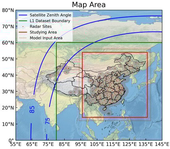
Figure 1.
Area coverage of different products. The blue lines indicate the satellite zenith angle, the green rectangle indicates the L1 AHI product boundary, the red points indicate land-based radars, the gray shading indicates radars’ coverage, and the red rectangles indicate the study area.
2.2. Himawari-9 Data
The Himawari-9 satellite is a new-generation geostationary meteorological satellite equipped with the Advanced Himawari Imager (AHI). The AHI features 16 bands ranging from the visible to the infrared spectrum, with spatial resolutions ranging from 500 m to 2 km. These 16 bands include 3 visible bands, 3 near-infrared bands, and 10 infrared bands [11]. More channels enable the acquisition of more detailed meteorological information. Specifically, for water vapor detection, the AHI includes 3 bands to detect moisture at different altitude levels. Additionally, 3 infrared window channels are also present. The sub-satellite point of the Himawari-9 is located near 140.7°E above the equator. Geostationary meteorological satellites offer advantages such as large scanning ranges and fixed scanning intervals. They can cover the entire area of China. The contours of the 85° and 75° satellite zenith angles are shown in Figure 1. The satellite performed scans approximately every 10 min, close to the radar’s scanning interval of 6 min. Level-1 product data with an equal latitude–longitude resolution of 5 km were obtained from ftp.ptree.jaxa.jp. The product covered the region from 60°N to 60°S and from 80°E to 160°W, as indicated by the green line in Figure 1. Included in the data were the albedos of visible and near-infrared bands, the brightness temperature of infrared bands (TBB), and geographic information such as solar zenith angle and solar azimuth angle. To retrieve radar reflectivity during both day and night, we focused on the infrared bands, especially the infrared window channels and the water vapor channels.
2.3. Study Area
Information on the study area is presented in the map in Figure 1. Areas with large satellite zenith angles may experience image distortion. The distribution of radar sites across China is not uniform, with significantly fewer radars in the west compared to the east. To address this issue, we selected the red rectangle as the study area after combining all the detection areas. The specific latitude and longitude ranges were from 96°E to 136°E and from 14°N to 54°N. The spatial resolution for all datasets was standardized to 0.05 degrees, approximately 5 km. To mitigate potential boundary issues caused by the convolution process, the input array was extended by 2 degrees in each direction. The input range of the model is outlined by a red dashed box in Figure 1.
2.4. Deep Learning Model
Since our goal was to test the influence of latitude and of the diurnal cycle, we did not conduct extensive deep-learning model testing. After testing on several segmentation models including FCN (fully convolutional networks) [18], UNet [19], UNet++ [20], and SegNet (semantic segmentation network) [21], Unet++ was found to be the best, with the smallest RMSE. UNet++ was chosen as our research model for further experimentation. UNet is a commonly used image segmentation model and performs quite well when applied to medical images [19]. UNet++ is an upgraded version of UNet that incorporates numerous skip connections [20]. The U-Net++ model retains the U-Net’s encoder–decoder structure but introduces a nested skip connection mechanism (the dash arrow in the Unet++ model in Figure 2) to enhance feature representation. The convolution ‘X’ in the figure represents the tensors of each layer in the model. Typically, the tensors in a model are high-dimensional matrices. For example, in our case, the input tensor had dimensions of 880 × 880 × m × N, where ‘m’ represents the number of channels in the input data, which is dependent on the model setting. In this study, the value of ‘m’ was between 5 and 10. ‘N’ represents the number of samples.
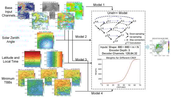
Figure 2.
Flowchart for the 4 deep learning models; the UNet++ model’s structure was referenced from Figure 1 in Zhou’s paper [20].
During the convolution process, each filter produces an output channel that captures different features from the input. The number of features can be manually set and is normally large. In the encoder–decoder process, the tensor will go through down-sampling and up-sampling. Down-sampling, also known as pooling, reduces the spatial dimensions of a tensor, and is typically performed to decrease the computational complexity. The tensor will turn to half or less of its original size after down-sampling. Up-sampling, also known as deconvolution or transposed convolution, is the reverse process of down-sampling.
Here, a 3-encoder–decoder-layer UNet++ model with an 880 × 880 grid input was established. The number of channels of the three encoder–decoder layers was set to 128, 64, and 32. During the encoder process, the tensors turned to 440 × 440 × 128 × N, 220 × 220 × 64 × N, and 110 × 110 × 32 × N; the reverse occurred during the decoder process.
The satellite data and other relevant data served as inputs to the model, while CREF served as the model’s output. All these elements were normalized individually. Details of the model settings are illustrated in the flowchart in Figure 2, including the thumbnail of the model inputs, the UNet++ structure, the line chart of the weighted loss function, and the model output. The data from the entire summer were divided into training sets and test sets. The data before the 20th of each month were used as the training set, and the remaining data served as the test set. A total of 2698 training samples and 1655 testing samples were generated.
The training process aimed to minimize the discrepancy between the inverted CREF and the actual CREF. The loss function serves as a quantitative measure of the discrepancy during the training, where the weight factors are the reciprocals of the probability density (PDF) of CREF. However, the probability density of strong echoes approaches zero, causing its reciprocal to tend toward infinity. So, we added a small value (0.001) to the denominator (Equation (1)). When the probability density of the echoes was relatively large, this value could be neglected, while when the probability density of the echoes approached zero, the value of 0.001 was the maximum value of the reciprocal of 1000.
The line chart of this function is represented by the red line in Figure 2.
We calculated the values for some typical CREF and listed them in Table 1. The statistical results showed that after CREF exceeded 48 dBZ, the PDF reached the order of 10−4, and the 1/PDF ratio exceeded 1000. Then, the PDF decreased rapidly, over 50 dBZ. After the small value of 0.001 was added, the weight (w) maintained a similar value to the original one below 30 dBZ, and beyond 50 dBZ, it approached1000 asymptotically.

Table 1.
A list of some typical CREF values and their weights.
The selection of a model input factors is crucial to the modeling process. We chose the inputs of the model based on the physical meanings of different satellite channels (Table 2). A total of 5 satellite channels were used, namely, channel 7 (IR 3.9 μm), channel 9 (IR 6.9 μm), channel 11 (IR 8.6 μm), channel 13 (IR 10.4 μm), and channel 15 (IR12.4 μm). The number in the subscript of the relative abbreviations indicates the wavelength at which each brilliance temperature was collected. The physical meanings of different variables were obtained from Zhuge and Mecikalki’s paper [22,23]. The infrared window band (channel 13, IR 10.4 μm) brightness temperature is an indicative index of cumulus cloud development. Generally, the lower the brightness temperature is, the more vigorously the cumulus cloud develops. However, the presence of stratocumulus clouds complicates this relationship. The cloud-top brightness temperature of stratocumulus clouds is generally low, but they rarely lead to precipitation. Therefore, and are introduced as input variables. These 2 TBB combinations are commonly used for stratocumulus cloud identification [24]. The thumbnails for the variables in Table 2 are displayed in the upper-left part of Figure 2.
Table 2.
Input Variables.
In order to enable the model to consider spatial and temporal variations, a total of 4 comparative experiments with different inputs were conducted. The models’ differences are listed in Table 3 and briefly shown in Figure 2.
Table 3.
Models setting.
Model 1 was the basic model using the variables listed in Table 1 as inputs. In model 2, we introduced the solar zenith angle (SZA). Since different latitudes have variations in SZA at different times, introducing the SZA can to some extent reflect spatiotemporal features. In model 3, we introduced the latitude and local time as inputs. It can be observed that the time and spatial information added in Model 2 and Model 3 was unrelated to the satellite images. The data added were relatively static and did not directly showcase the features of the TBBs. These two models were designed to determine whether the deep learning model could improve the results from this static geographical information, which was unrelated to the TBBs.
Finally, in Model 4, we incorporated spatiotemporal features of the infrared cloud image directly. In the context of infrared cloud images, lower temperatures are associated with higher and thicker clouds. Conversely, high temperatures often indicate clear skies, and in such cases, the detection is performed at the ground surface level. We selected the minimum temperature at each pixel as the feature to be incorporated, because this temperature could represent the lower temperature limit of clouds at that location. The minimum temperature at each pixel for all the channels at each time was calculated using the training datasets. TBB maps of a total of were generated as static data to be used as the model input. The model output will be described in Section 3.2.
3. Results
3.1. Features of Different Variables
Precipitation exhibits a strong daily cycle and varies by latitude. Before constructing deep learning models, it is essential to analyze the precipitation data distribution. Temporal distribution and spatial distribution were considered for both CREF and TBB.
3.1.1. Radar Composite Reflectivity
The distribution of CREF at different times was calculated, and the results are shown in Figure 3. It is evident that the CREF distribution exhibited a pronounced diurnal cycle, and the cycle for different reflectivity levels varied. The distribution of CREF probability was extremely uneven, showing an exponential decline from weak to strong reflectivity (Figure 3c). The proportion of CREF over 35 dBz was very small, only about 0.04%. An interesting phenomenon can be observed related to the difference in the diurnal cycle between strong and weak reflectivity (Figure 3a,b). Strong reflectivity had a bimodal distribution, with peaks at 8:00 and 16:00, respectively. The afternoon peak was stronger than the morning one. Weak reflectivity, on the other hand, was predominant during nighttime, which was mainly caused by long and moderate rainfall at night.
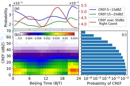
Figure 3.
Radar reflectivity distribution. (a) The frequency of different CREF values and their diurnal cycles. The blue line represents CREF between 5 and 15 dBZ, the green line represents CREF between 15 and 25 dBZ, and the red line represents CREF over 35 dBZ. Note that this figure is a dual-y-axis plot, with the red line referring to the coordinates on the right. (b) Grid shading of CREF frequency of occurrence for different reflectivity values at different times. (c) Statistical distribution of different reflectivity values.
Besides varying with the diurnal cycle, reflectivity also varies with latitude. We calculated the probability of CREF over 35 dBz at different latitudes and different times. The probabilities over land and sea were calculated separately, and the results are shown in Figure 4a,b. The blank areas in the figure indicate no radar coverage at that latitude, where the sample count was zero. Three rain belts can be observed depending on the latitude, over land. The southern one was the strongest, located at 17.5°N to 22.5°N. The peak of strong probability was in the afternoon, suggesting that heavy precipitation in southern China usually occurs in the afternoon. The middle rain belt, located at 27.5°N to 35°N, had different distribution characteristics. It showed two peaks, in the early morning and in the afternoon, and the early-morning peak was stronger, probably related to the stationary front located in this area. The northern belt was much weaker than the other two. The probability over the sea was much different; limited by the radar’s coverage, most of the samples were from near-shore areas. The number of samples is printed on the left side of the image. Storm probability over the sea also showed different belts located in southern and middle China. The peak of storm probability was at noon.
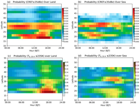
Figure 4.
Latitude- and time-related storm probability. (a) CREF ≥ 35 dBz over land. (b) CREF ≥ 35 dBz over sea. (c) ≤ 235 K over land. (d) ≤ 235 K over sea.
3.1.2. Brightness Temperature
The TBB of IR 10.4 μm is an indicator of the cloud-top temperature, which is closely linked to cloud height. The colder the TBB, the more vigorous the cloud development. TBBs colder than 235 K can be recognized as mature convection [25,26]. We calculated the probability of measuring a TBB colder than 235 K by time and latitude. To keep consistent with the radar CREF statistical results, a radar cover mask was applied to the TBB datasets. The statistical results for land and sea are shown in Figure 4c,d. Some interesting observations can be made by comparing these result to the CREF ones.
We found some common patterns. Firstly, the three belts were obvious in the TBB results, coinciding with the CREF results. Secondly, two peaks were found in the middle and northern belts. However, some different patterns drew our attention. Firstly, the two peaks over middle China had opposite strengths compared to the CREF peaks. In the TBB results, the afternoon peal was stronger than the early-morning one. Secondly, the northern belt was only slightly smaller than the middle belt (Figure 4a), which differed from the CREF results (Figure 4c). In the CREF figure, the probability in the northern belt was about half of that in the middle belt.
We conducted a statistical analysis of the minimum cloud-top brightness temperatures at different latitudes and examined the diurnal variation of the minimum cloud-top brightness temperature. Figure 5 illustrates the statistical results of IR 10.4 μm. The minimum TBB tended to be lower in the south and higher in the north (Figure 5a). Next, we calculated the minimum temperature for each specific latitude at each time in the diurnal cycle (Figure 5b). The same trend is observed in the diurnal variation cycle graph. Simultaneously, it can be observed that in the northern regions, the difference between maximum and minimum temperature was more significant, with extremely high TBBs around noon, and low TBBs at night.
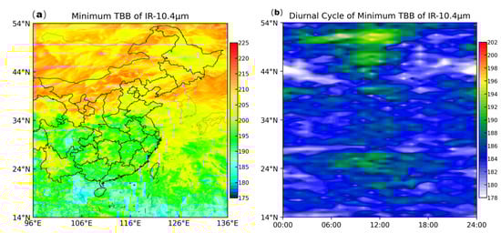
Figure 5.
(a) Distribution of the minimum TBBs of IR 10.4 μm. (b) Diurnal cycle of minimum TBBs of IR 10.4 μm; the temperature is the minimum TBB for each specific latitude at each time in the diurnal cycle.
3.2. Model Output
In this study, we compared and evaluated the outputs of all four models. Here, we present the products during the occurrence of the super typhoon Doksuri. Figure 6 displays the TBBs of IR 10.4 and the radar composite reflectivity (CREF), along with the outputs from the four models.
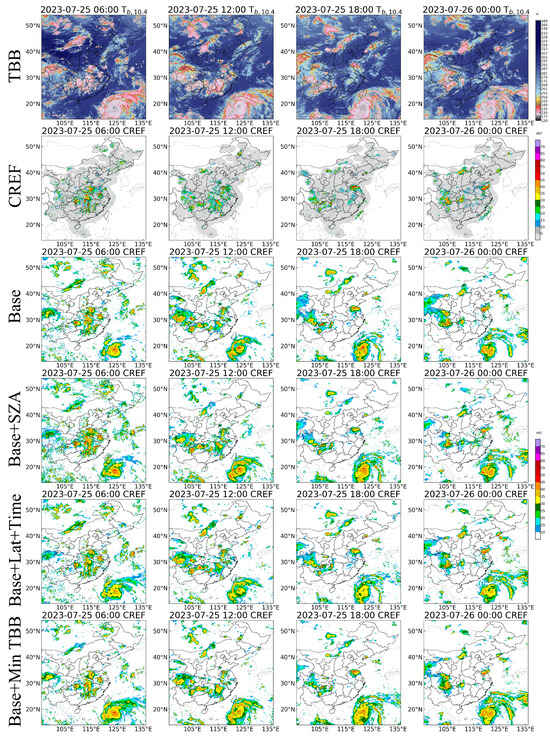
Figure 6.
Model outputs for super typhoon Doksuri. First row for ; second row for land-based CREF; third row for base model output (model 1); fourth row for the model using SZA (model 2); fifth row for the model considering latitude and local time (model 3); sixth row for the model using the minimum TBB (model 4).
Comparing the images of TBB and CREF revealed a rather complex relationship between the two. Cold cloud areas were typically much larger than the regions with strong radar echoes. This difference was particularly noticeable in northern regions, where many cloud structures lacked corresponding radar echoes. The limited penetration capability of the infrared band in the northern regions contributed to this observation, even though all four models successfully retrieved the CREF data, distinguishing these cloud structures. This validated the effectiveness of the retrieval method. Using this approach, CREF maps over the sea could be generated. From these maps, intense convective areas associated with typhoon Doksuri became evident.
Qualitatively comparing the results to the actual CREF, it can be observed that the strong echo areas predicted by the deep learning models were larger than their actual counterparts. This was mainly due to the restricted penetration capability of the infrared band; many highly vigorous cloud structures exhibited similar features in satellite cloud images. In addition, the four models exhibited different characteristics. The base model tended to overestimate CREF in the northern regions compared to the other models, possibly due to the absence of latitude considerations. The model with SZA provided better simulations of extreme values in the centers of strong storms compared to other models, but it tended to overestimate the area covered by strong echoes. The CREF obtained by the model with latitude and time was generally weaker than that of the other models. The extreme CREF generated by the model with minimum TBB was not as well-defined as those obtained with the model with SZA, but the reflectivity was much cleaner. The other models generated many weak reflectivity regions that were not present in the actual radar image, while the model with minimum TBB was able to eliminate these false signals. This can be observed from the reflectivity image of the Ningxia Province (areas around 114°E, 38°N) at 06:00. This was mainly obtained with Model 4 considering the distribution of TBBs at different locations and times. The minimum TBB plays the role of background plate and eliminated some systematic bias.
4. Discussion
4.1. Spatial Analysis
To quantitatively evaluate the results of the different tested models, we calculated the RMSE of CREF for each pixel and drew an RMSE map (Figure 7). The RMSE deviation was relatively small between 35°N and 45°N, but a larger deviation was observed in South China below 30°N. Three areas in the figure that require special attention are (1) Southeast China, (2) Northeast China, (3) the Sichuan Basin, (Around 100°E, 30°N).
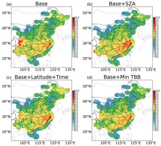
Figure 7.
Map of the RMSE for all 4 models. (a) Base model, (b) model using SZA, (c) model considering latitude and local time, (d) model using the minimum TBB.
The southeast region of China experiences more precipitation and a higher frequency of intense echoes, leading to relatively larger errors. The model using SZA showed the highest RMSE for Southeast China. The base model and the model based on latitude and time performed equally. Notably, the model using the minimum TBB performed the best.
The performance of the model based on the minimum TBB was better in the Northeast region. The model based on latitude and time performed the worst in the Northeast region. The values of RMSE and the area with a high RMSE were the larger among those obtained with the four models. In addition, the base model exhibited an unusually high RMSE for the Sichuan Basin region.
Overall, in the three regions of interest, Models 1–3 had their own shortcomings. In contrast, Model 4 demonstrated excellent performance across a wide range of areas.
4.2. Diurnal Cycle Analysis
In order to analyze the diurnal variation of the retrieved errors, we calculated the RMSE and critical success index (CSI, Equation (2)) of different models at different times. The results were show in Figure 8. The RMSE was primarily used to assess the overall accuracy of the inversion, while the 35 dBz CSI was mainly used to evaluate the accuracy of strong echoes.
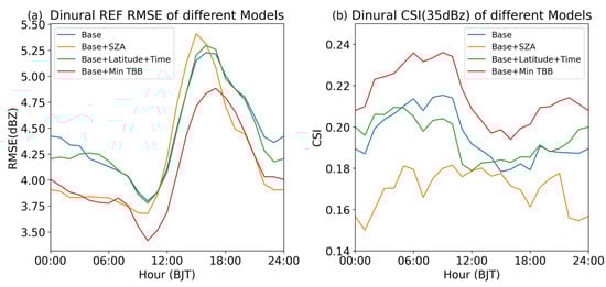
Figure 8.
Diurnal cycle of RMSE (a) and 35 dBz CSI (b).
The equation of CSI refers to Equation (2). The following variables were used:
Hits: Pixels where retrieved CREF and land-based CREF occurred.
Misses: Pixels where retrieved CREF did not occur, but land-based CREF occurred.
False alarms: Pixels where retrieved CREF occurred, but land-based CREF did not occur.
All test datasets were evaluated, and the RMSE and 35 dBz CSI were calculated at each hour. The results are shown in Figure 8. In all models, the model incorporating the minimum TBB performed the best. It consistently reduced the RMSE and improved the CSI across all hours of the day, while the other three models had advantages at different times. This suggested to us the following: (1) simply feeding static geographic information to deep learning models and adding new feature parameters to the model may not improve the models’ accuracy; (2) the minimum TBB can be considered as a background factor and is an effective variable that can improve a model’s performance; (3) although there are variations in the relationship between TBB and CREF at different locations and times, introducing the right variables can enhance a model.
4.3. Distribution Analysis
To enhance the evaluation of the model outputs, a two-dimensional histogram of observed and retrieved CREF values was obtained. Alongside this, several other metrics were calculated, including correlation coefficient, accuracy, and RMSE of echoes over 10 dBZ. Here, accuracy is defined as absolute deviation less than or equal to 3 dBZ. The results are show in Figure 9. The summary of all evaluation results can be found in Table 4.
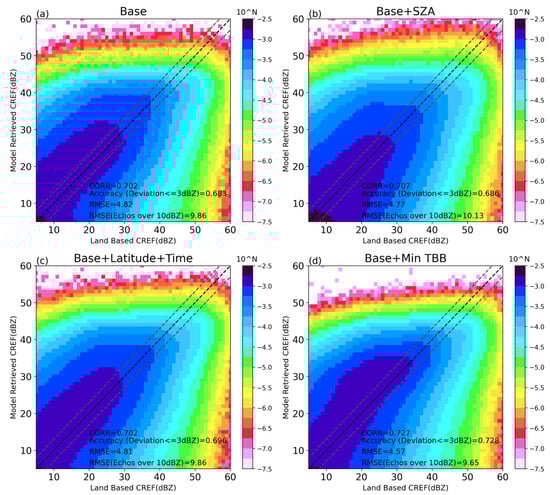
Figure 9.
Comparisons of the occurrence frequency between land-based CREF and the retrieved CREF. The frequency is in logarithmic scale. (a) Base model. (b) Model using SZA. (c) Model based on latitude and local time. (d) Model with minimum TBB.
Table 4.
Error metrics of the 4 models.
The frequency distribution maps were obtained from all the test datasets. Due to differences in data magnitude, we applied a logarithmic transformation during the plotting process. In Figure 9, some common results can be observed. It appeared that the model tended to overestimate echoes below 20 dBZ and underestimate extremely strong echoes (over 50 dBZ). The proportion of strong echoes was relatively lower than that observed. The model based on SZA performed better than the others in the presence of strong echoes. However, overall, the retrieved results of the model with minimum TBB aligned better with the observations. In the graph, it can be observed that the deep green portion (frequency over 10 × 10−3) is more elongated, indicating a better fit.
The quantitative evaluation results indicated that the correlation coefficients of all models were all around 0.7, approximately. The model based on minimum TBB was slightly superior to the others, with a correlation coefficient of 0.727. We obtained similar results in terms of accuracy, RMSE, and RMSE of the precipitation echoes. Model 4 outperformed thew others in all four evaluation metrics.
5. Conclusions
In this article, we utilized the Himawari-9 satellite to establish a method for reconstructing radar CREF over land and sea. Through the spatiotemporal analysis of CREF and TBB, we identified three rain belts in the Chinese region. We found a clear diurnal cycle of convective probability over all three rain belts. However, the diurnal cycle of convective activity showed differences in its manifestation on the CREF and TBB maps. On the CREF map, server convection tended to happen in the morning, while on the TBB map, it tended to happen in the afternoon.
We employed UNet++ to experiment with different input variables and tested four models. The results showed that the UNet++ model could reconstruct radar CREF well. The inversion accuracy of all models was around 70%, and the correlation coefficients were around 0.7. Among the tested models, the model based on minimum TBB was the best as regards all error metrics, with a correlation coefficient of 0.727, accuracy of 0.728, RMSE of 4.57, RMSE for echoes over 10 dBZ of 9.65, and CSI of 35 dBZ of 0.215.
Our results showed that the base model failed to balance the features across different regions, especially in the inversion process in the Sichuan area. The model with SZA exhibited better inversion performance for extreme strong echoes (CREF over 50 dBZ). However, at the same time, it also exhibited the largest RMSE. The model based on latitude and time was relatively mediocre. While it could improve the inversion performance in certain regions, on a national scale, there was no significant improvement. The model with minimum TBB performed the best. After adding the minimum TBB of different channels as a background parameter, the model’s retrieved CREF RMSE was lower than those of the other models in both spatial dimension and diurnal cycle. The 35 dBZ CSI was improved too. This indicated that there are indeed differences in the relationship between satellite and radar reflectivity in terms of both region and time. Further research, such as on the QPE of satellite data, needs to take this in consideration.
Author Contributions
Conceptualization, B.W. and C.Y.G.; Methodology, B.W.; Formal analysis, B.W.; Writing—original draft, B.W.; Writing—review & editing, C.Y.G. All authors have read and agreed to the published version of the manuscript.
Funding
This research was funded by the Jiangsu Funding Program for Excellent Postdoctoral Talent (grant no. 2023ZB012) and the State Key Laboratory of Atmospheric Boundary Layer Physics and Atmospheric Chemistry (grant no. LAPC-KF-2023-05).
Data Availability Statement
The satellite data presented in this study are available on the internet. The other data presented in this study are available on request from the author.
Acknowledgments
We would like to thank the anonymous reviewers for their thoughtful and constructive suggestions and comments.
Conflicts of Interest
The authors declare no conflicts of interest.
References
- Yu, X.; Zheng, Y. Advances in Severe Convection Research and Operation in China. J. Meteorol. Res. 2020, 34, 189–217. [Google Scholar] [CrossRef]
- Villarini, G.; Krajewski, W.F. Review of the different sources of uncertainty in single polarization radar-based estimates of rainfall. Surv. Geophys. 2010, 31, 107–129. [Google Scholar] [CrossRef]
- Houze, R.A.; Biggerstaff, M.I.; Rutledge, S.A.; Smull, B.F. Interpretation of Doppler Weather Radar Displays of Midlatitude Mesoscale Convective Systems. Bull. Am. Meteorol. Soc. 1989, 70, 608–619. [Google Scholar] [CrossRef]
- Doviak, R.; Zrnic, S. Doppler Radar and Weather Observations; Courier Corporation: North Chelmsford, MA, USA, 2006. [Google Scholar]
- Roberts, R.D.; Rutledge, S. Nowcasting storm initiation and growth using GOES-8 and WSR-88D data. Weather Forecast. 2003, 18, 562–584. [Google Scholar] [CrossRef]
- Ravuri, S.; Lenc, K.; Willson, M.; Kangin, D.; Lam, R.; Mirowski, P.; Fitzsimons, M.; Athanassiadou, M.; Kashem, S.; Madge, S.; et al. Skilful precipitation nowcasting using deep generative models of radar. Nature 2021, 597, 672–677. [Google Scholar] [CrossRef] [PubMed]
- Wang, Y.; Long, M.; Wang, J.; Gao, Z.; Yu, P.S. PredRNN: Recurrent Neural Networks for Predictive Learning using Spatiotemporal LSTMs. In Advances in Neural Information Processing Systems; Curran Associates, Inc.: Red Hook, NY, USA, 2017; Volume 30. [Google Scholar]
- Zhang, Y.; Long, M.; Chen, K.; Xing, L.; Jin, R.; Jordan, M.I.; Wang, J. Skilful nowcasting of extreme precipitation with NowcastNet. Nature 2023, 619, 526–532. [Google Scholar] [CrossRef] [PubMed]
- Bauer, P.; Thorpe, A.; Brunet, G. The quiet revolution of numerical weather prediction. Nature 2015, 525, 47–55. [Google Scholar] [CrossRef]
- Sheng, C.; Gao, S.; Xue, M. Short-range prediction of a heavy precipitation event by assimilating Chinese CINRAD-SA radar reflectivity data using complex cloud analysis. Meteorol. Atmos. Phys. 2006, 94, 167–183. [Google Scholar] [CrossRef]
- Bessho, K.; Date, K.; Hayashi, M.; Ikeda, A.; Imai, T.; Inoue, H.; Kumagai, Y.; Miyakawa, T.; Murata, H.; Ohno, T.; et al. An introduction to Himawari-8/9—Japan’s new-generation geostationary meteorological satellites. J. Meteorol. Soc. Jpn. Ser. II 2016, 94, 151–183. [Google Scholar] [CrossRef]
- Kuligowski, R.; Yu, H.; Hao, Y.; Zhang, Y. Improvements to the GOES-R rainfall rate algorithm. J. Hydrometeorol. 2016, 17, 1693–1704. [Google Scholar] [CrossRef]
- Sun, R.; Yuan, H.; Liu, X.; Jiang, X. Evaluation of the latest satellite–gauge precipitation products and their hydrologic applications over the Huaihe River basin. J. Hydrol. 2016, 536, 302–319. [Google Scholar] [CrossRef]
- Tang, G.; Clark, M.P.; Papalexiou, S.M.; Ma, Z.; Hong, Y. Have satellite precipitation products improved over last two decades? A comprehensive comparison of GPM IMERG with nine satellite and reanalysis datasets. Remote Sens. Environ. 2019, 240, 111697. [Google Scholar] [CrossRef]
- Duan, M.; Xia, J.; Yan, Z.; Han, L.; Zhang, L.; Xia, H.; Yu, S. Reconstruction of the radar reflectivity of convective storms based on deep learning and himawari-8 observations. Remote Sens. 2021, 13, 3330. [Google Scholar] [CrossRef]
- Sun, F.; Li, B.; Min, M.; Qin, D. Deep learning-based radar composite reflectivity factor estimations from fengyun-4a geostationary satellite observations. Remote Sens. 2021, 13, 2229. [Google Scholar] [CrossRef]
- Wang, G.; Liu, L.; Ding, Y. Improvement of radar quantitative precipitation estimation based on real-time adjustments to Z-R relationships and inverse distance weighting correction schemes. Adv. Atmos. Sci. 2012, 29, 575–584. [Google Scholar] [CrossRef]
- Shelhamer, E.; Long, J.; Darrell, T. Fully Convolutional Networks for Semantic Segmentation. IEEE Trans. Pattern Anal. Mach. Intell. 2017, 39, 640–651. [Google Scholar] [CrossRef] [PubMed]
- Ronneberger, O.; Fischer, P.; Brox, T. U-Net: Convolutional Networks for Biomedical Image Segmentation. In Proceedings of the Medical Image Computing and Computer-Assisted Intervention—MICCAI 2015: 18th International Conference, Munich, Germany, 5–9 October 2015; pp. 234–241. [Google Scholar]
- Zhou, Z.; Siddiquee, M.M.R.; Tajbakhsh, N.; Liang, J. UNet++: A Nested U-Net Architecture for Medical Image Segmentation. In Deep Learning in Medical Image Analysis and Multimodal Learning for Clinical Decision Support; Springer: Berlin/Heidelberg, Germany, 2018. [Google Scholar] [CrossRef]
- Badrinarayanan, V.; Kendall, A.; Cipolla, R. Segnet: A Deep Convolutional Encoder-Decoder Architecture for Image Segmentation. IEEE Trans. Pattern Anal. Mach. Intell. 2017, 39, 2481–2495. [Google Scholar] [CrossRef] [PubMed]
- Zhuge, X.; Zou, X. Summertime convective initiation nowcasting over southeastern China based on advanced himawari imager observations. J. Meteorol. Soc. Jpn. Ser. II 2018, 96, 337–353. [Google Scholar] [CrossRef]
- Mecikalski, J.R.; Bedka, K.M. Forecasting convective initiation by monitoring the evolution of moving cumulus in daytime GOES imagery. Mon. Weather Rev. 2006, 134, 49–78. [Google Scholar] [CrossRef]
- Lee, S.; Han, H.; Im, J.; Jang, E.; Lee, M.-I. Detection of deterministic and probabilistic convection initiation using Himawari-8 Advanced Himawari Imager data. Atmos. Meas. Tech. 2017, 10, 1859–1874. [Google Scholar] [CrossRef]
- Laing, A.G.; Fritsch, J.M. The Large-scale environments of the global populations of mesoscale convective complexes. Mon. Weather Rev. 2000, 128, 2756–2776. [Google Scholar] [CrossRef]
- Vila, D.A.; Machado, L.A.T.; Laurent, H.; Velasco, I. Forecast and tracking the evolution of cloud clusters (ForTraCC) using satellite infrared imagery: Methodology and validation. Weather Forecast. 2008, 23, 233–245. [Google Scholar] [CrossRef]
Disclaimer/Publisher’s Note: The statements, opinions and data contained in all publications are solely those of the individual author(s) and contributor(s) and not of MDPI and/or the editor(s). MDPI and/or the editor(s) disclaim responsibility for any injury to people or property resulting from any ideas, methods, instructions or products referred to in the content. |
© 2023 by the authors. Licensee MDPI, Basel, Switzerland. This article is an open access article distributed under the terms and conditions of the Creative Commons Attribution (CC BY) license (https://creativecommons.org/licenses/by/4.0/).