
Evaluation and Analysis of Remote Sensing-Based Approach for Salt Marsh Monitoring

 ,
,  ,
,
Abstract
:
1. Introduction
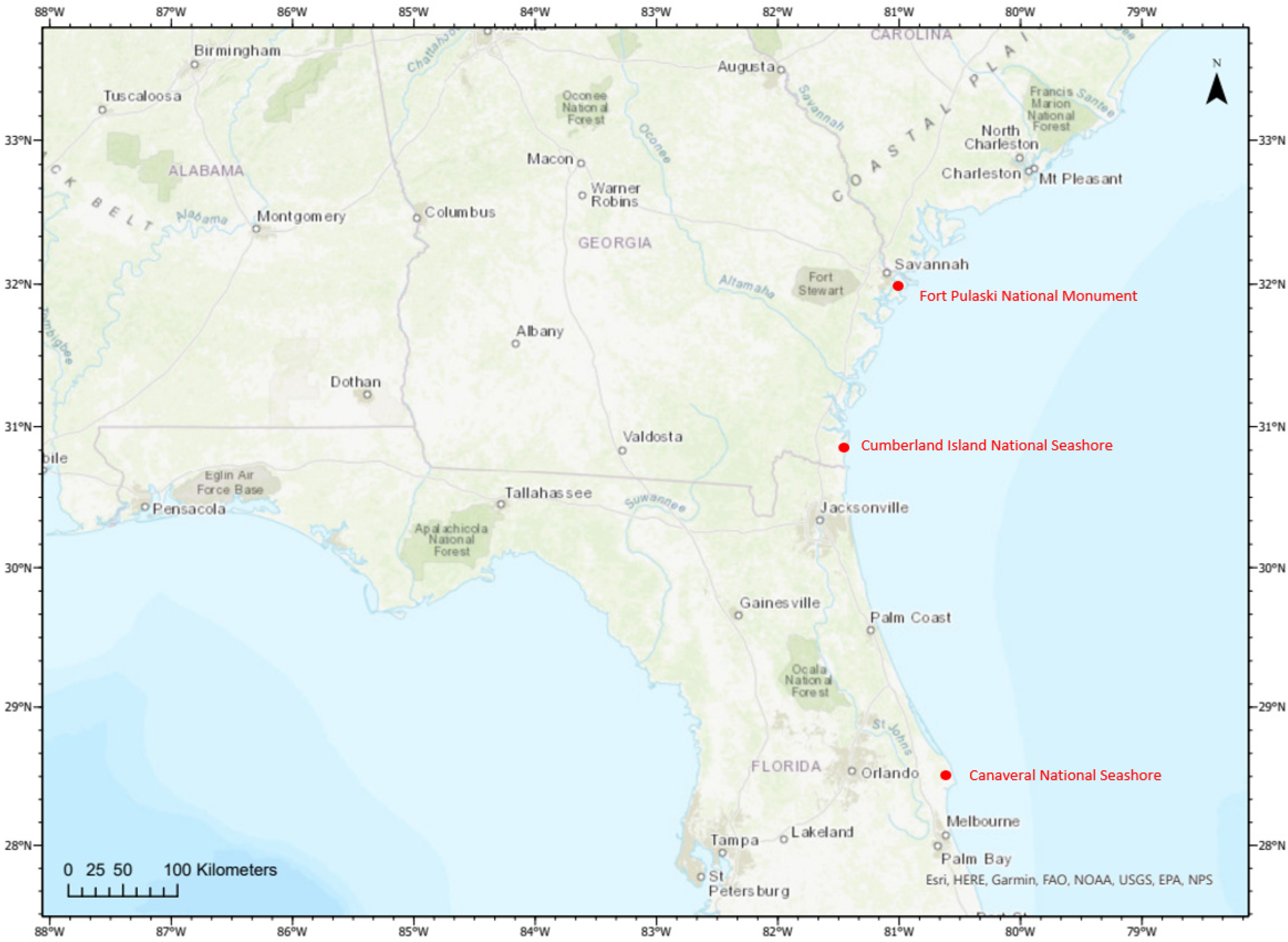
2. Study Area
3. Methodology
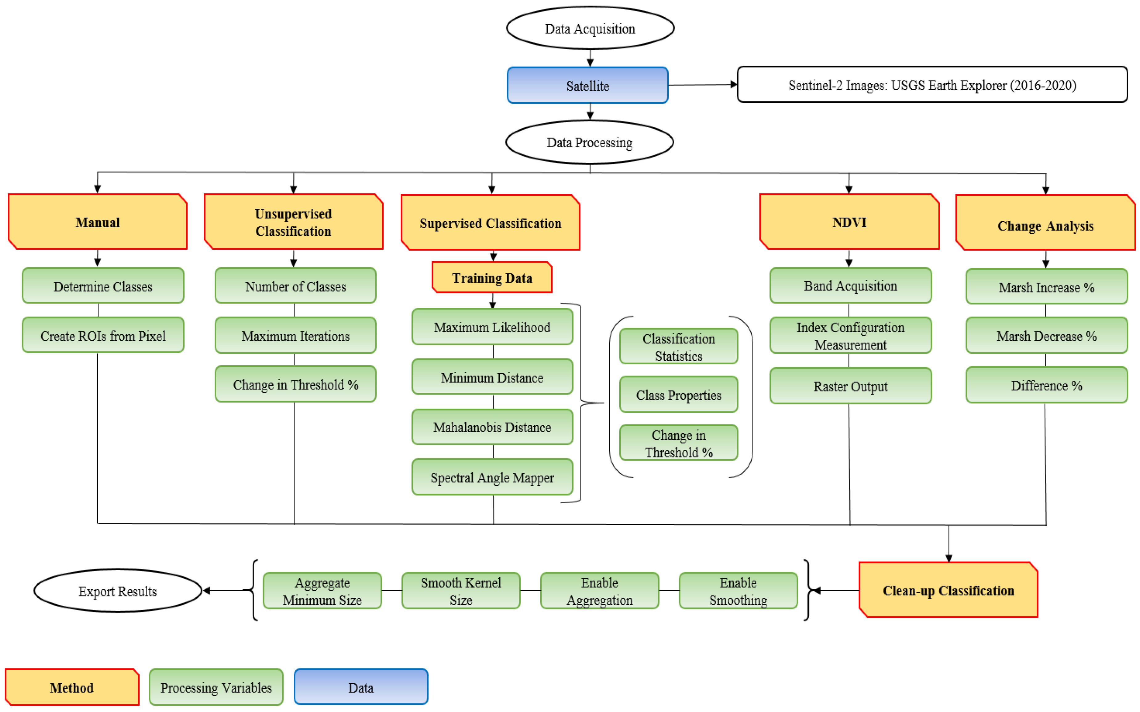
3.1. Data Acquisition
3.2. Data Processing
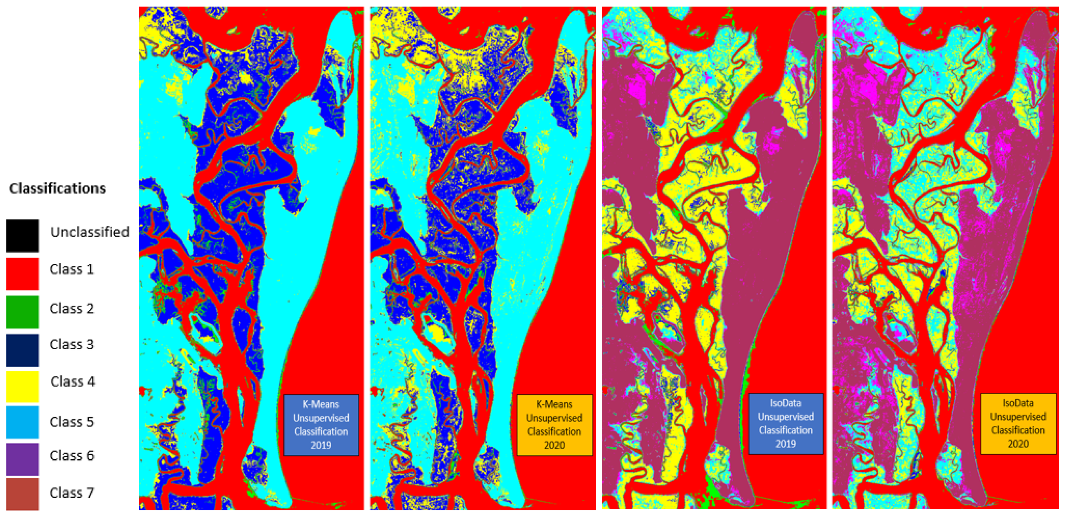
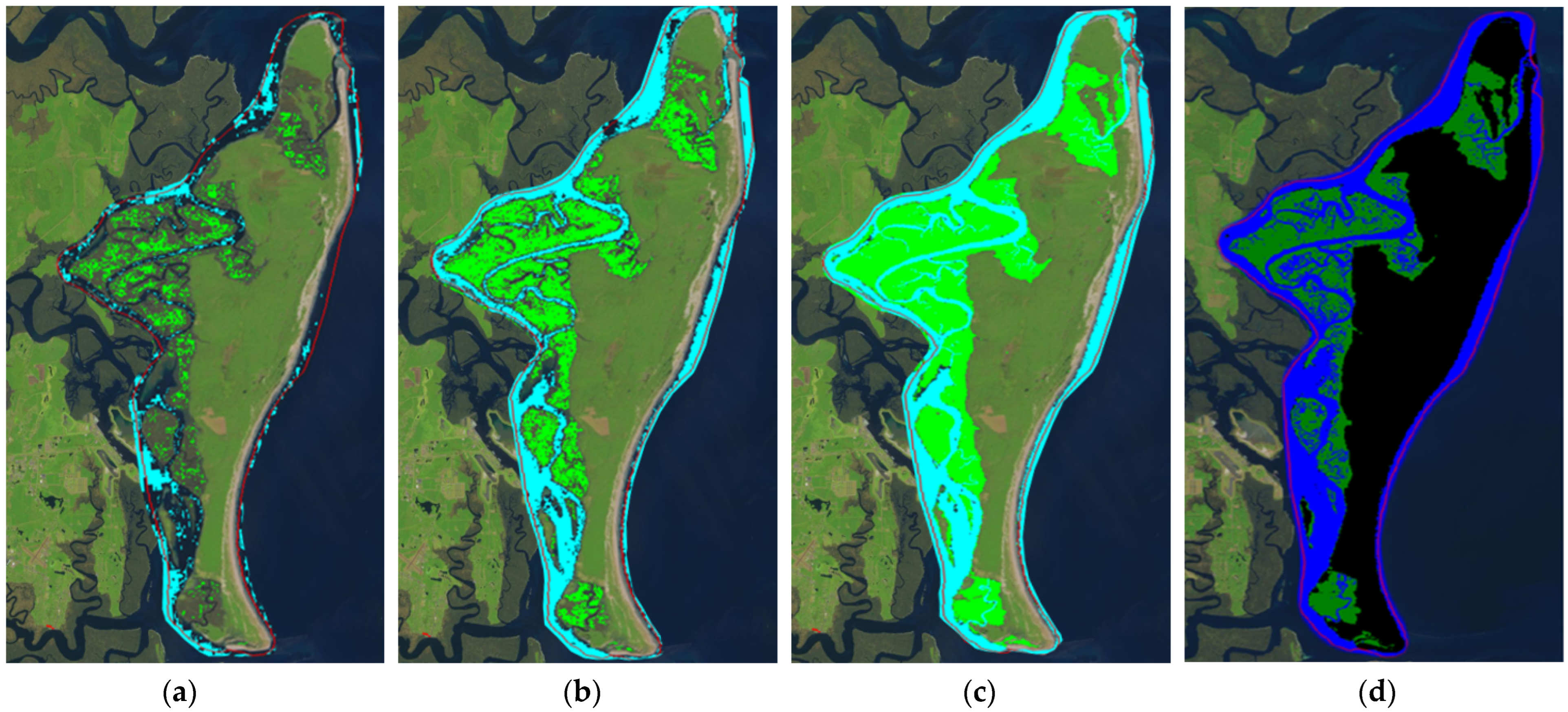
3.3. Unsupervised Classification
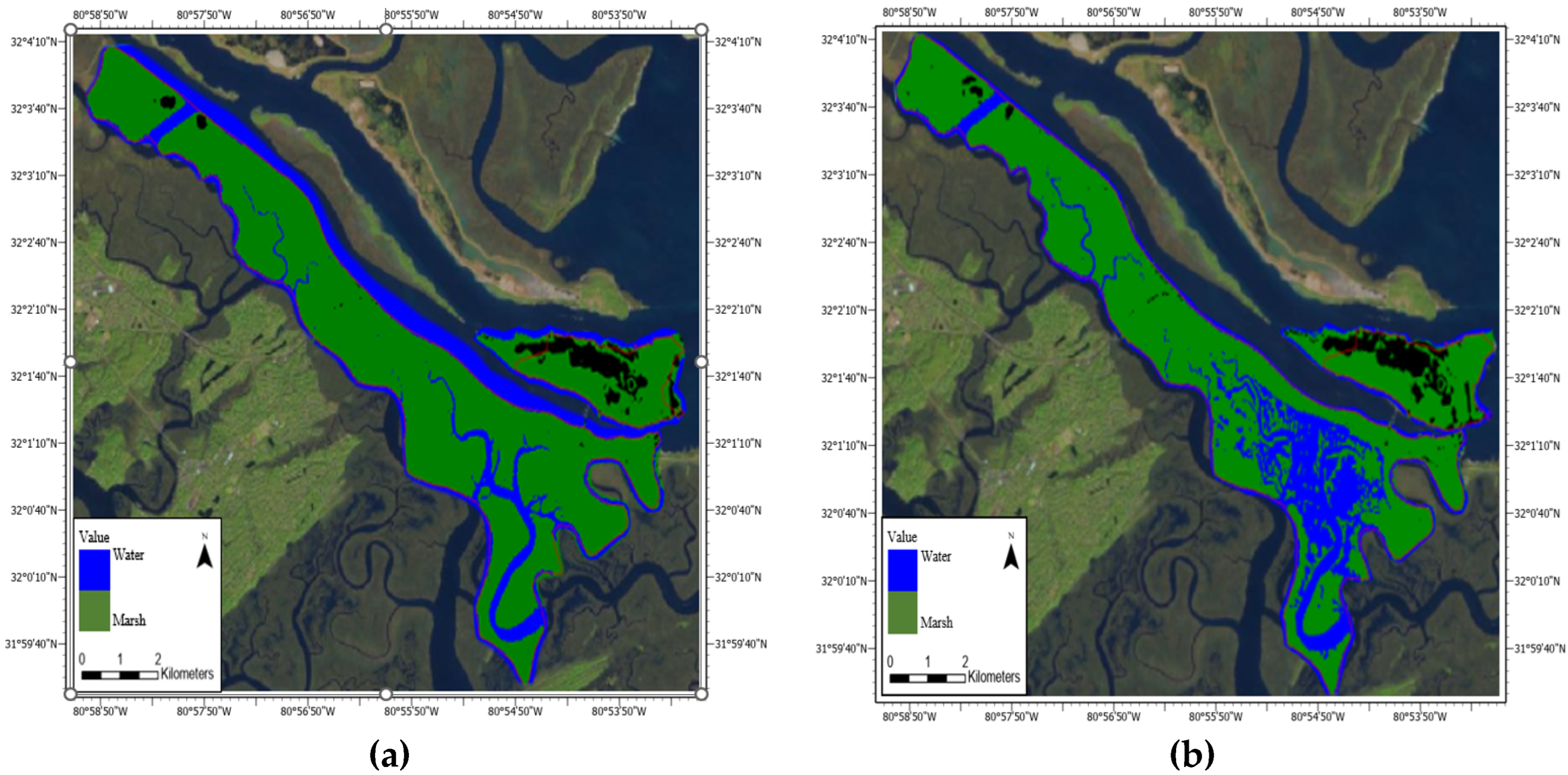
3.4. Supervised Classification
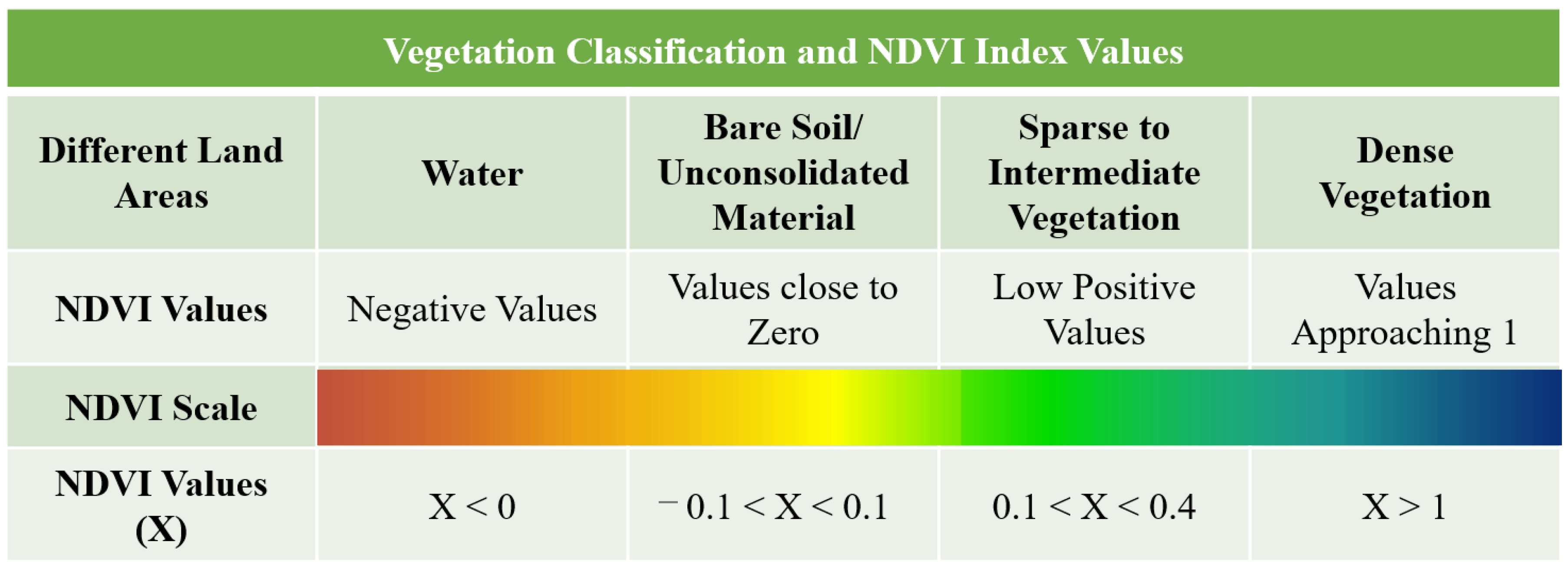
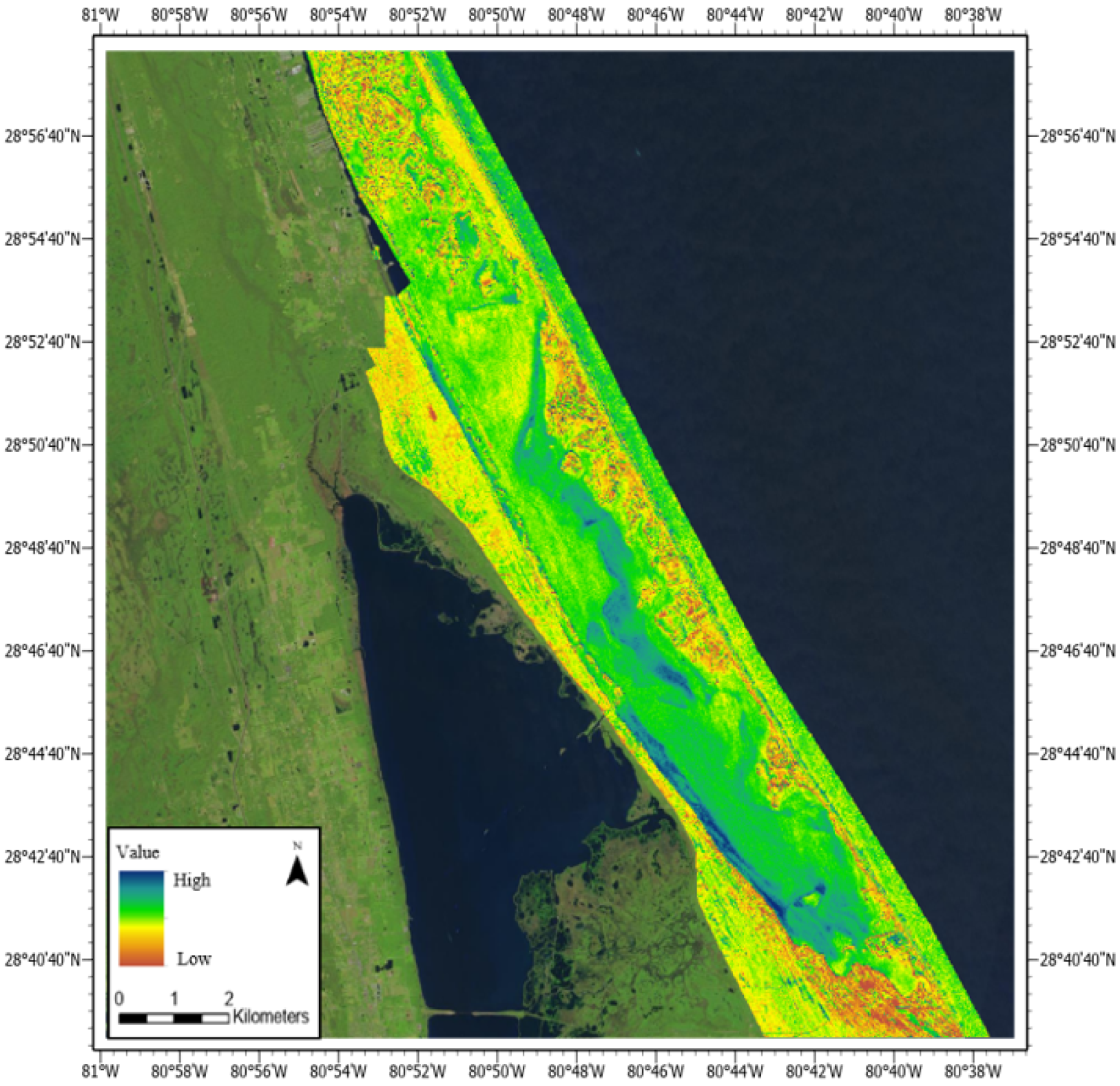
3.5. Normalized Difference Vegetation Index (NDVI)
3.6. Change Detection Analysis
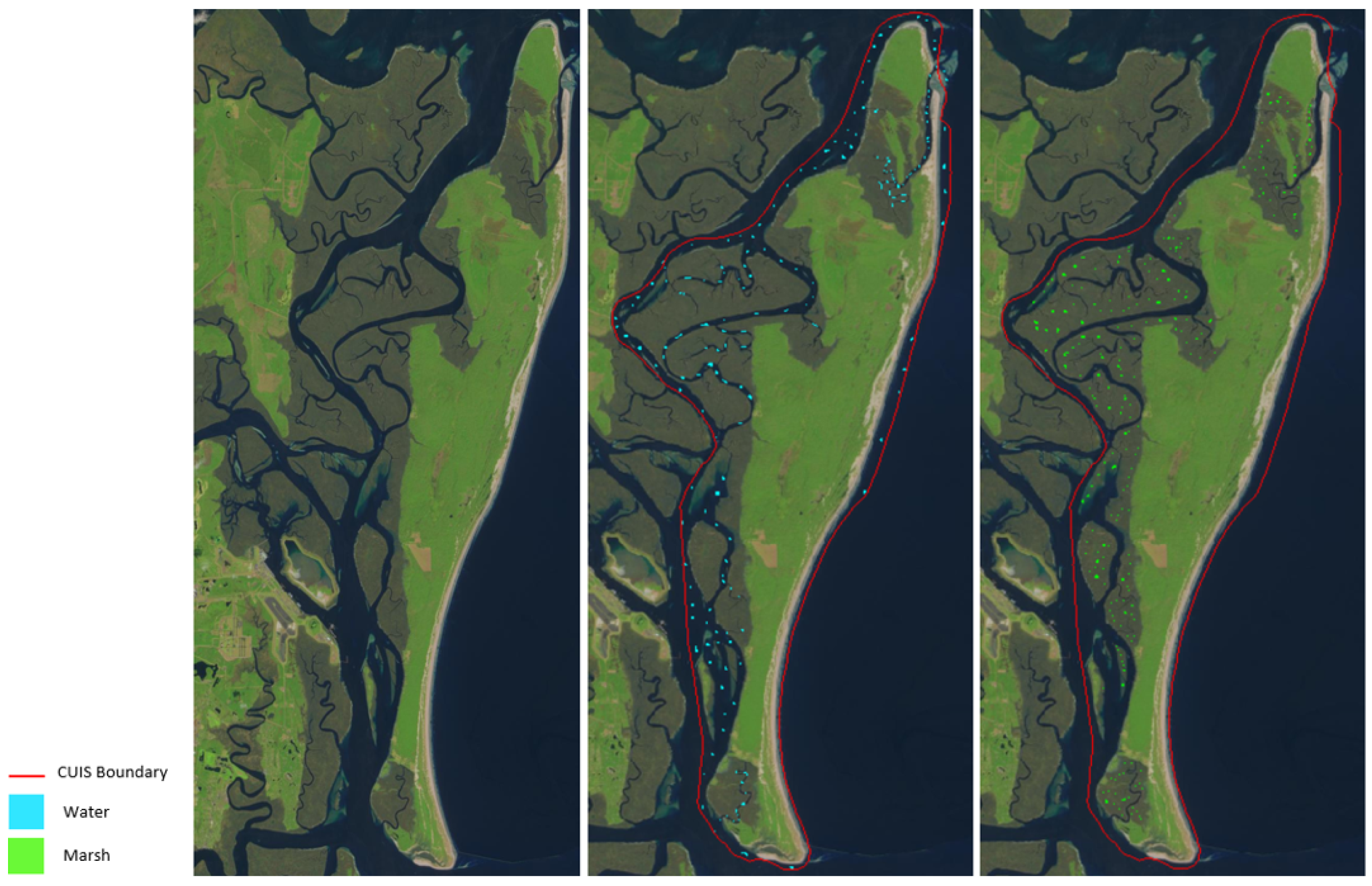
3.7. Validation
4. Results
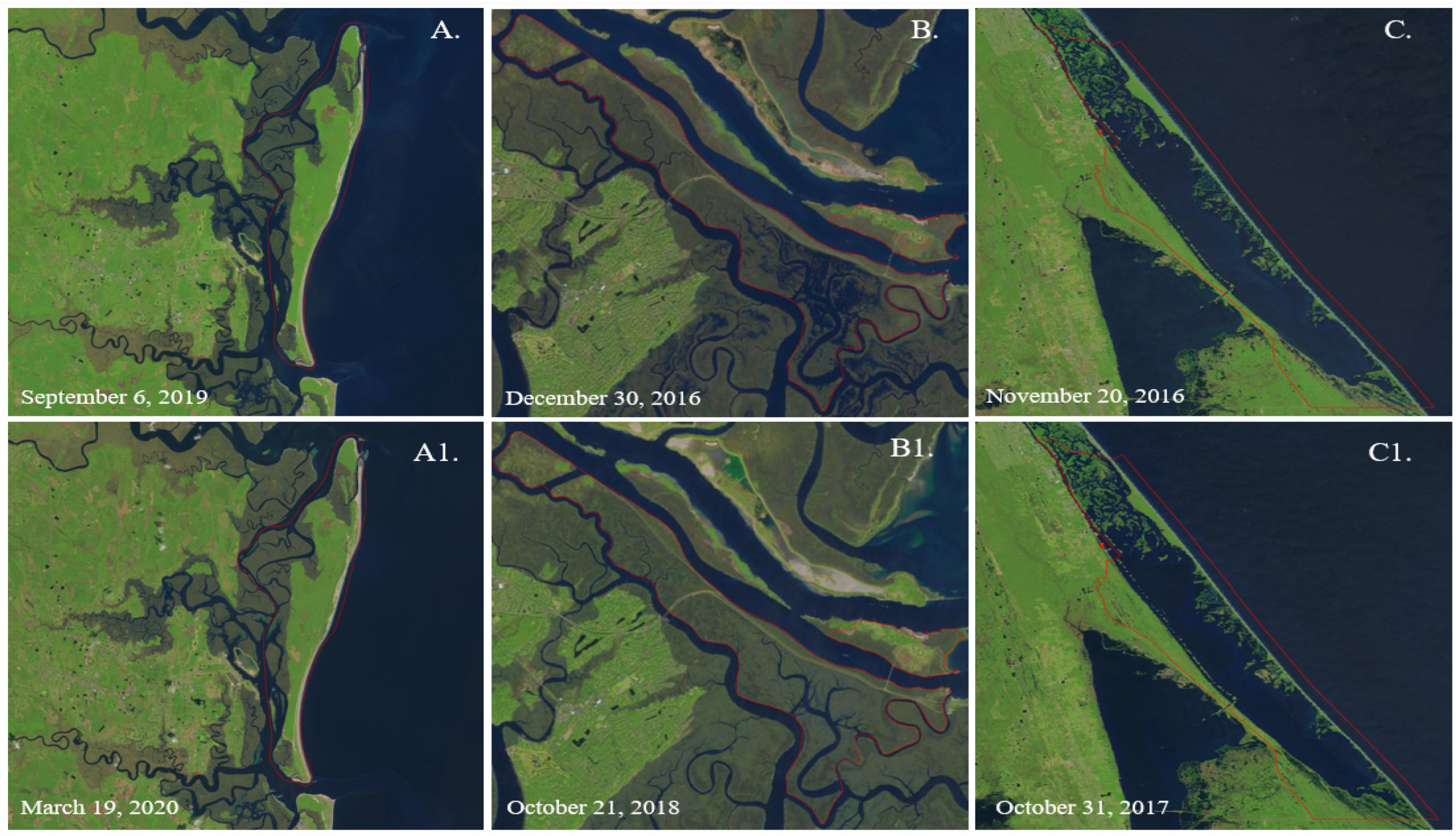
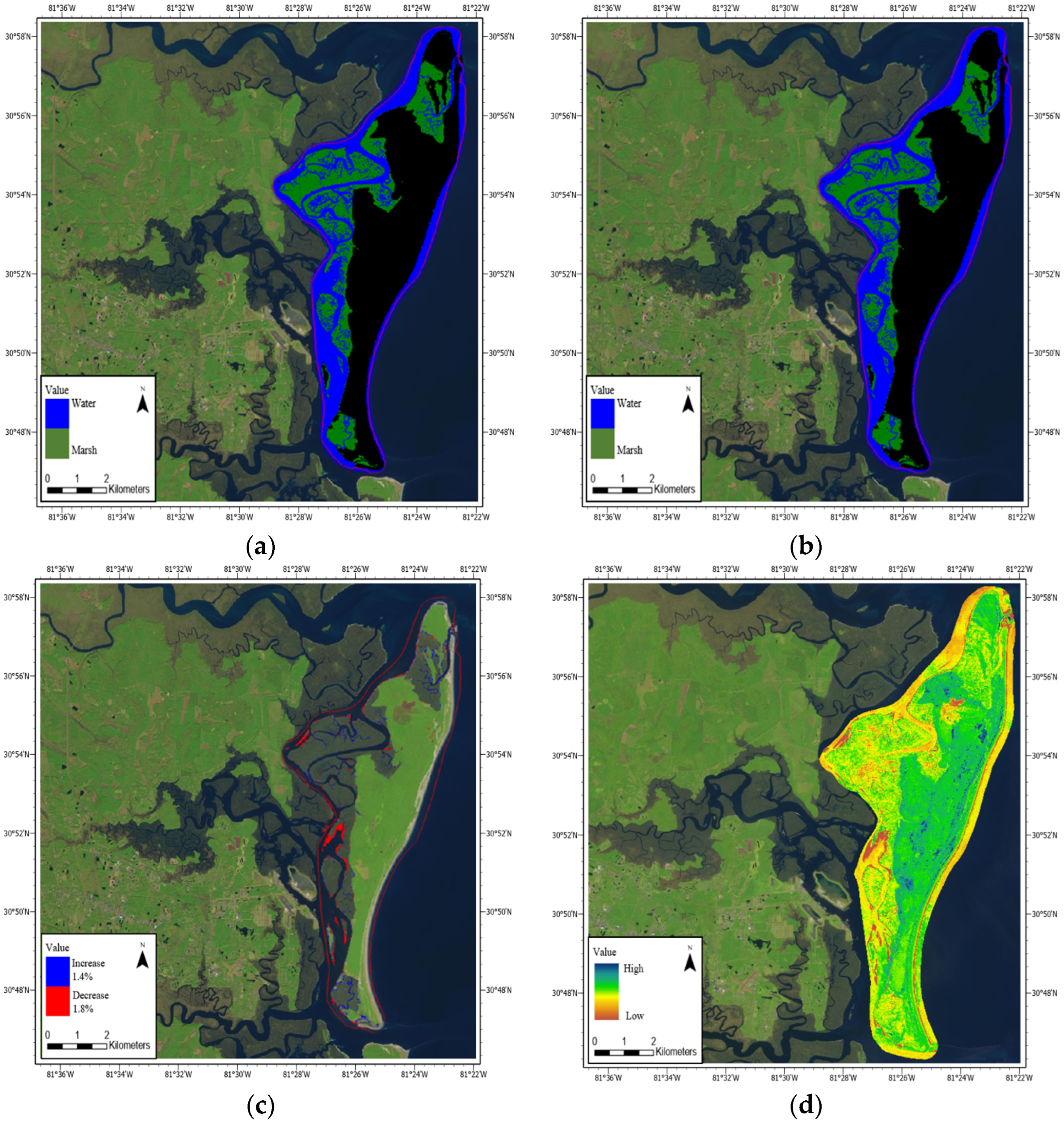
4.1. Cumberland Island National Seashore
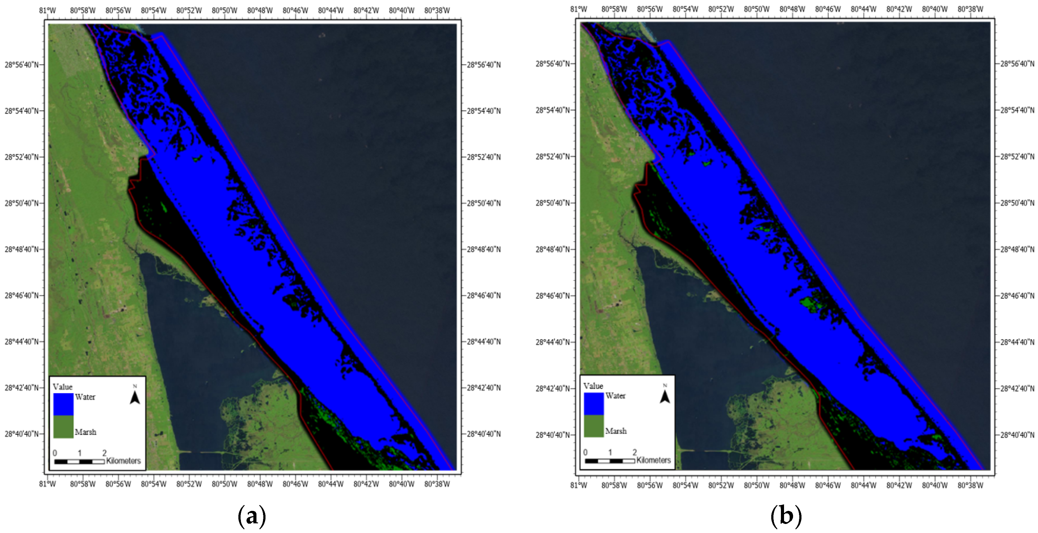
4.2. Canaveral National Seashore
4.3. Supervised Classification Accuracy
4.4. Tidal Influence
5. Discussion
6. Conclusions
Author Contributions
Funding
Data Availability Statement
Acknowledgments
Conflicts of Interest
References
- Barbier, E.B.; Hacker, S.D.; Kennedy, C.; Koch, E.W.; Stier, A.C.; Silliman, B.R. The value of estuarine and coastal ecosystem services. Ecol. Monogr. 2011, 81, 169–193. [Google Scholar] [CrossRef]
- Crosby, S.C.; Sax, D.F.; Palmer, M.E.; Booth, H.S.; Deegan, L.A.; Bertness, M.D.; Leslie, H.M. Salt marsh persistence is threatened by predicted sea-level rise. Estuar. Coast. Shelf Sci. 2016, 181, 93–99. [Google Scholar] [CrossRef]
- Simas, T.; Nunes, J.P.; Ferreira, J.G. Effects of global climate change on coastal salt marshes. Ecol. Model. 2001, 139, 1–15. [Google Scholar] [CrossRef]
- Stagg, C.L.; Osland, M.J.; Moon, J.A.; Feher, L.C.; Laurenzano, C.; Lane, T.C.; Jones, W.R.; Hartley, S.B. Extreme precipitation and flooding contribute to sudden vegetation dieback in a coastal salt marsh. Plants 2021, 10, 1841. [Google Scholar] [CrossRef]
- Alber, M.; Swenson, E.M.; Adamowicz, S.C.; Mendelssohn, I.A. Salt marsh dieback: An overview of recent events in the US. Estuar. Coast. Shelf Sci. 2008, 80, 1–11. [Google Scholar] [CrossRef]
- Orson, R.; Panageotou, W.; Leatherman, S.P. Response of tidal salt marshes of the US Atlantic and Gulf coasts to rising sea levels. J. Coast. Res. 1985, 1, 29–37. [Google Scholar]
- Schwarz, C.; van Rees, F.; Xie, D.; Kleinhans, M.G.; van Maanen, B. Salt marshes create more extensive channel networks than mangroves. Nat. Commun. 2022, 13, 2017. [Google Scholar] [CrossRef]
- Mariotti, G.; Canestrelli, A. Long-term morphodynamics of muddy backbarrier basins: Fill in or empty out? Water Resour. Res. 2017, 53, 7029–7054. [Google Scholar] [CrossRef]
- Guimond, J.; Tamborski, J. Salt marsh hydrogeology: A review. Water 2021, 13, 543. [Google Scholar] [CrossRef]
- Byrd, K.B.; Kelly, M. Salt marsh vegetation response to edaphic and topographic changes from upland sedimentation in a Pacific estuary. Wetlands 2006, 26, 813–829. [Google Scholar] [CrossRef]
- Craft, C.B.; Seneca, E.D.; Broome, S.W. Vertical accretion in microtidal regularly and irregularly flooded estuarine marshes. Estuar. Coast. Shelf Sci. 1993, 37, 371–386. [Google Scholar] [CrossRef]
- Halpern, B.S.; Walbridge, S.; Selkoe, K.A.; Kappel, C.V.; Micheli, F.; d’Agrosa, C.; Bruno, J.F.; Casey, K.S.; Ebert, C.; Fox, H.E.; et al. A global map of human impact on marine ecosystems. Science 2008, 319, 948–952. [Google Scholar] [CrossRef] [PubMed]
- Hartig, E.K.; Gornitz, V.; Kolker, A.; Mushacke, F.; Fallon, D. Anthropogenic and climate-change impacts on salt marshes of Jamaica Bay, New York City. Wetlands 2002, 22, 71–89. [Google Scholar] [CrossRef]
- Kennish, M.J. Coastal salt marsh systems in the US: A review of anthropogenic impacts. J. Coast. Res. 2001, 17, 731–748. [Google Scholar]
- South Atlantic Salt Marsh Initiative. Executive Summary: Marsh Forward—A Regional Plan for the Future of the South Atlantic Coast’s Million-Acre Salt Marsh Ecosystem. 2023. Available online: https://www.marshforward.org (accessed on 5 August 2023).
- Crooks, S.; Herr, D.; Tamelander, J.; Laffoley, D.; Vandever, J. Mitigating Climate Change through Restoration and Management of Coastal Wetlands and Near-Shore Marine Ecosystems: Challenges and Opportunities; The World Bank: Washington, DC, USA, 2011. [Google Scholar]
- Duarte, C.M.; Dennison, W.C.; Orth, R.J.; Carruthers, T.J. The charisma of coastal ecosystems: Addressing the imbalance. Estuaries Coasts 2008, 31, 233–238. [Google Scholar] [CrossRef]
- Mcowen, C.J.; Weatherdon, L.V.; Van Bochove, J.W.; Sullivan, E.; Blyth, S.; Zockler, C.; Stanwell-Smith, D.; Kingston, N.; Martin, C.S.; Spalding, M.; et al. A global map of saltmarshes. Biodivers. Data J. 2017, 5, e11764. [Google Scholar] [CrossRef]
- IPBES (Intergov. Sci. Policy Platf. Biodivers. Ecosyst. Serv.). The Assessment Report on Land Degradation and Restoration. Rep., IPBES, Bonn, Ger, 2018. Available online: http://www.ipbes.net (accessed on 18 June 2023).
- Campbell, A.D.; Fatoyinbo, L.; Goldberg, L.; Lagomasino, D. Global hotspots of salt marsh change and carbon emissions. Nature 2022, 612, 701–706. [Google Scholar] [CrossRef]
- Fretwell, S.; Wagner, A.; Lee, A. “A Million Acres of ‘Priceless’ Marshes Protect NC, SC, GA. Will They Perish in Rising Tides?” The News and Observer. 2021. Available online: https://pulitzercenter.org/stories/million-acres-priceless-marshes-protect-nc-sc-ga-will-they-perish-rising-tides (accessed on 18 June 2023).
- Campbell, A.; Wang, Y. High spatial resolution remote sensing for salt marsh mapping and change analysis at Fire Island National Seashore. Remote Sens. 2019, 11, 1107. [Google Scholar] [CrossRef]
- DiGiacomo, A.E.; Bird, C.N.; Pan, V.G.; Dobroski, K.; Atkins-Davis, C.; Johnston, D.W.; Ridge, J.T. Modeling salt marsh vegetation height using unoccupied aircraft systems and structure from motion. Remote Sens. 2020, 12, 2333. [Google Scholar] [CrossRef]
- Roughgarden, J.; Running, S.W.; Matson, P.A. What does remote sensing do for ecology? Ecology 1991, 72, 1918–1922. [Google Scholar] [CrossRef]
- Belluco, E.; Camuffo, M.; Ferrari, S.; Modenese, L.; Silvestri, S.; Marani, A.; Marani, M. Mapping salt-marsh vegetation by multispectral and hyperspectral remote sensing. Remote Sens. Environ. 2006, 105, 54–67. [Google Scholar] [CrossRef]
- Silvestri, S.; Marani, M.; Marani, A. Hyperspectral remote sensing of salt marsh vegetation, morphology and soil topography. Phys. Chem. Earth Parts A/B/C 2003, 28, 15–25. [Google Scholar] [CrossRef]
- Farris, A.S.; Defne, Z.; Ganju, N.K. Identifying salt marsh shorelines from remotely sensed elevation data and imagery. Remote Sens. 2019, 11, 1795. [Google Scholar] [CrossRef]
- Zhang, M.; Ustin, S.L.; Rejmankova, E.; Sanderson, E.W. Monitoring Pacific coast salt marshes using remote sensing. Ecol. Appl. 1997, 7, 1039–1053. [Google Scholar] [CrossRef]
- Fagherazzi, S.; Marani, M.; Blum, L.K. The Ecogeomorphology of Tidal Marshes; American Geophysical Union: Washington, DC, USA, 2004. [Google Scholar]
- Silvestri, S.; Marani, M. Salt-marsh vegetation and morphology: Basic physiology, modelling and remote sensing observations. Ecogeomorphology Tidal Marshes 2004, 59, 5–25. [Google Scholar]
- Day, J.W.; Christian, R.R.; Boesch, D.M.; Yáñez-Arancibia, A.; Morris, J.; Twilley, R.R.; Naylor, L.; Schaffner, L.; Stevenson, C. Consequences of climate change on the ecogeomorphology of coastal wetlands. Estuaries Coasts 2008, 31, 477–491. [Google Scholar] [CrossRef]
- Scavia, D.; Field, J.C.; Boesch, D.F.; Buddemeier, R.W.; Burkett, V.; Cayan, D.R.; Fogarty, M.; Harwell, M.A.; Howarth, R.W.; Mason, C.; et al. Climate change impacts on US coastal and marine ecosystems. Estuaries 2002, 25, 149–164. [Google Scholar] [CrossRef]
- Kirwan, M.L.; Mudd, S.M. Response of salt-marsh carbon accumulation to climate change. Nature 2012, 489, 550–553. [Google Scholar] [CrossRef]
- Schuerch, M.; Vafeidis, A.; Slawig, T.; Temmerman, S. Modeling the influence of changing storm patterns on the ability of a salt marsh to keep pace with sea level rise. J. Geophys. Res. Earth Surf. 2013, 118, 84–96. [Google Scholar] [CrossRef]
- Mwamba, M.J.; Torres, R. Rainfall effects on marsh sediment redistribution, North Inlet, South Carolina, USA. Mar. Geol. 2002, 189, 267–287. [Google Scholar] [CrossRef]
- Valiela, I.; Teal, J.M.; Volkmann, S.; Shafer, D.; Carpenter, E.J. Nutrient and particulate fluxes in a salt marsh ecosystem: Tidal exchanges and inputs by precipitation and groundwater 1. Limnol. Oceanogr. 1978, 23, 798–812. [Google Scholar] [CrossRef]
- Sanderson, E.W.; Ustin, S.L.; Foin, T.C. The influence of tidal channels on the distribution of salt marsh plant species in Petaluma Marsh, CA, USA. Plant Ecol. 2000, 146, 29–41. [Google Scholar] [CrossRef]
- Tempest, J.A.; Harvey, G.L.; Spencer, K.L. Modified sediments and subsurface hydrology in natural and recreated salt marshes and implications for delivery of ecosystem services. Hydrol. Process. 2015, 29, 2346–2357. [Google Scholar] [CrossRef]
- Hughes, A.L.; Wilson, A.M.; Morris, J.T. Hydrologic variability in a salt marsh: Assessing the links between drought and acute marsh dieback. Estuar. Coast. Shelf Sci. 2012, 111, 95–106. [Google Scholar] [CrossRef]
- Wilson, A.M.; Evans, T.; Moore, W.; Schutte, C.A.; Joye, S.B.; Hughes, A.H.; Anderson, J.L. Groundwater controls ecological zonation of salt marsh macrophytes. Ecology 2015, 96, 840–849. [Google Scholar] [CrossRef] [PubMed]
- Giri, C.; Ochieng, E.; Tieszen, L.L.; Zhu, Z.; Singh, A.; Loveland, T.; Masek, J.; Duke, N. Status and distribution of mangrove forests of the world using earth observation satellite data. Glob. Ecol. Biogeogr. 2011, 20, 154–159. [Google Scholar] [CrossRef]
- Vo, Q.T.; Oppelt, N.; Leinenkugel, P.; Kuenzer, C. Remote sensing in mapping mangrove ecosystems—An object-based approach. Remote Sens. 2013, 5, 183–201. [Google Scholar] [CrossRef]
- Berger, M.; Moreno, J.; Johannessen, J.A.; Levelt, P.F.; Hanssen, R.F. ESA’s sentinel missions in support of Earth system science. Remote Sens. Environ. 2012, 120, 84–90. [Google Scholar] [CrossRef]
- Dale, J.; Burnside, N.G.; Hill-Butler, C.; Berg, M.J.; Strong, C.J.; Burgess, H.M. The use of unmanned aerial vehicles to determine differences in vegetation cover: A tool for monitoring coastal wetland restoration schemes. Remote Sens. 2020, 12, 4022. [Google Scholar] [CrossRef]
- Gorelick, N.; Hancher, M.; Dixon, M.; Ilyushchenko, S.; Thau, D.; Moore, R. Google Earth Engine: Planetary-scale geospatial analysis for everyone. Remote Sens. Environ. 2017, 202, 18–27. [Google Scholar] [CrossRef]
- Campbell, A.D.; Wang, Y. Salt marsh monitoring along the mid-Atlantic coast by Google Earth Engine enabled time series. PLoS ONE 2020, 15, e0229605. [Google Scholar] [CrossRef] [PubMed]
- Yeo, S.; Lafon, V.; Alard, D.; Curti, C.; Dehouck, A.; Benot, M.L. Classification and mapping of saltmarsh vegetation combining multispectral images with field data. Estuar. Coast. Shelf Sci. 2020, 236, 106643. [Google Scholar] [CrossRef]
- McManamay, R.H. Vegetation Mapping at Cumberland Island National Seashore; Natural Resource Report NPS/SECN/NRR—2017/1511; National Park Service: Fort Collins, CO, USA, 2017.
- McManamay, R.H.; Curtis, A.C.; Heath, S.C. Vegetation Mapping at Fort Pulaski National Monument; Natural Resource Report NPS/SECN/NRR—2013/718; National Park Service: Fort Collins, CO, USA, 2013.
- Cotton, D.L.; Adams, B.P.; O’Hare, N.K.; Bernardes, S.; Jordan, T.R.; Madden, M. Vegetation Mapping at Canaveral National Seashore: Photointerpretation Key and Final Vegetation Map; Natural Resource Report NPS/SECN/NRR—2020/2084; National Park Service: Fort Collins, CO, USA, 2020.
- Davey, C.A.; Redmond, K.T.; Simeral, D.B. Weather and Climate Inventory, National Park Service, Southeast Coast Network; Natural Resource Technical Report NPS/SECN/NRTR—2007/010; National Park Service: Fort Collins, CO, USA, 2007.
- Pieschke, R.L. U.S. Geological Survey Distribution of European Space Agency’s Sentinel-2 Data: U.S. Geological Survey Fact Sheet 2017–3026; U.S. Geological Survey: Sioux Falls, SD, USA, 2017; 2p. [CrossRef]
- European Space Agency-Sentinel. 2022. Sentinel User Guides Product Type. Available online: https://sentinels.copernicus.eu/web/sentinel/user-guides/sentinel-2-msi/product-types/level-1c (accessed on 21 July 2023).
- Aslan, A.; Rahman, A.F.; Warren, M.W.; Robeson, S.M. Mapping spatial distribution and biomass of coastal wetland vegetation in Indonesian Papua by combining active and passive remotely sensed data. Remote Sens. Environ. 2016, 183, 65–81. [Google Scholar] [CrossRef]
- Giri, C.; Pengra, B.; Zhu, Z.; Singh, A.; Tieszen, L.L. Monitoring mangrove forest dynamics of the Sundarbans in Bangladesh and India using multi-temporal satellite data from 1973 to 2000. Estuar. Coast. Shelf Sci. 2007, 73, 91–100. [Google Scholar] [CrossRef]
- Yagoub, M.M.; Kolan, G.R. Monitoring coastal zone land use and land cover changes of Abu Dhabi using remote sensing. J. Indian Soc. Remote Sens. 2006, 34, 57–68. [Google Scholar] [CrossRef]
- NV5 Geospatial. 2022. ENVI Classification. Available online: https://www.nv5geospatialsoftware.com/docs/Classification (accessed on 21 July 2023).
- Jones, H.G.; Vaughan, R.A. Remote Sensing of Vegetation: Principles, Techniques, and Applications; Oxford University Press: Oxford, UK, 2010. [Google Scholar]
- Korchagina, I.A.; Goleva, O.G.; Savchenko, Y.Y.; Bozhikov, T.S. The use of geographic information systems for forest monitoring. In Journal of Physics: Conference Series; IOP Publishing: Bristol, UK, 2020; Volume 1515, p. 032077. [Google Scholar]
- Huang, S.; Tang, L.; Hupy, J.P.; Wang, Y.; Shao, G. A commentary review on the use of normalized difference vegetation index (NDVI) in the era of popular remote sensing. J. For. Res. 2021, 32, 1–6. [Google Scholar] [CrossRef]
- Nardin, W.; Taddia, Y.; Quitadamo, M.; Vona, I.; Corbau, C.; Franchi, G.; Staver, L.W.; Pellegrinelli, A. Seasonality and characterization mapping of restored tidal marsh by NDVI imageries coupling UAVs and multispectral camera. Remote Sens. 2021, 13, 4207. [Google Scholar] [CrossRef]
- Otsu, N. A threshold selection method from gray-level histograms. IEEE Trans. Syst. Man Cybermetrics 1979, 9, 62–66. [Google Scholar] [CrossRef]
- Xu, R.; Zhao, S.; Ke, Y. A simple phenology-based vegetation index for mapping invasive spartina alterniflora using Google Earth engine. IEEE J. Sel. Top. Appl. Earth Obs. Remote Sens. 2020, 14, 190–201. [Google Scholar] [CrossRef]
- Jia, M.; Wang, Z.; Mao, D.; Ren, C.; Wang, C.; Wang, Y. Rapid, robust, and automated mapping of tidal flats in China using time series Sentinel-2 images and Google Earth Engine. Remote Sens. Environ. 2021, 255, 112285. [Google Scholar] [CrossRef]
- Liu, Y.; Zhou, M.; Zhao, S.; Zhan, W.; Yang, K.; Li, M. Automated extraction of tidal creeks from airborne laser altimetry data. J. Hydrol. 2015, 527, 1006–1020. [Google Scholar] [CrossRef]
- Kuleli, T.; Guneroglu, A.; Karsli, F.; Dihkan, M. Automatic detection of shoreline change on coastal Ramsar wetlands of Turkey. Ocean. Eng. 2021, 38, 1141–1149. [Google Scholar] [CrossRef]
- Calzadilla Pérez, A.; Damen, M.C.J.; Geneletti, D.; Hobma, T.W. Monitoring a recent delta formation in a tropical coastal wetland using remote sensing and GIS. Case study: Guapo River delta, Laguna de Tacarigua, Venezuela. Environ. Dev. Sustain. 2002, 4, 201–219. [Google Scholar] [CrossRef]
- Ogburn, M.B.; Alber, M. An investigation of salt marsh dieback in Georgia using field transplants. Estuaries Coasts 2006, 29, 54–62. [Google Scholar] [CrossRef]
- Stagg, C.L.; Mendelssohn, I.A. Restoring ecological function to a submerged salt marsh. Restor. Ecol. 2010, 18, 10–17. [Google Scholar] [CrossRef]
- Fagherazzi, S.; Kirwan, M.L.; Mudd, S.M.; Guntenspergen, G.R.; Temmerman, S.; D’Alpaos, A.; Van De Koppel, J.; Rybczyk, J.M.; Reyes, E.; Craft, C.; et al. Numerical models of salt marsh evolution: Ecological, geomorphic, and climatic factors. Rev. Geophys. 2012, 50. [Google Scholar] [CrossRef]
- Fagherazzi, S.; Hannion, M.; D’Odorico, P. Geomorphic structure of tidal hydrodynamics in salt marsh creeks. Water Resour. Res. 2008, 44. [Google Scholar] [CrossRef]
- Leung, L.Y.; Prasad, R. Potential Impacts of Accelerated Climate Change: Third Annual Report of Work (No. PNNL-27452-Rev. 1); Pacific Northwest National Lab (PNNL): Richland, WA, USA, 2019.
- Pham, T.D.; Xia, J.; Ha, N.T.; Bui, D.T.; Le, N.N.; Takeuchi, W. A review of remote sensing approaches for monitoring blue carbon ecosystems: Mangroves, seagrasses and salt marshes during 2010–2018. Sensors 2019, 19, 1933. [Google Scholar] [CrossRef]
- Michener, W.K.; Blood, E.R.; Bildstein, K.L.; Brinson, M.M.; Gardner, L.R. Climate change, hurricanes and tropical storms, and rising sea level in coastal wetlands. Ecol. Appl. 1997, 7, 770–801. [Google Scholar] [CrossRef]


| Supervised Classification Scheme Accuracy % | ||||
|---|---|---|---|---|
| Classifications | Marsh Pixels (270) | Marsh Accuracy % | Water Pixels (207) | Water Accuracy % |
| Maximum Likelihood | 243 | 90% | 207 | 99% |
| Minimum Distance | 239 | 89% | 197 | 95% |
| Spectral Angle Mapper | 234 | 87% | 168 | 81% |
| Mahalanobis Distance | 62 | 23% | 8 | 43% |
| Validation Accuracy % | |||
|---|---|---|---|
| Features | Input Points (ROIs) | Conferred Points | Accuracy % |
| Cumberland Island National Seashore | |||
| Salt Marsh | 270 | 242 | 90% |
| Water | 207 | 205 | 99% |
| Canaveral National Seashore | |||
| Salt Marsh | 12 | 9 | 75% |
| Water | 102 | 100 | 98% |
| Fort Pulaski National Monument | |||
| Salt Marsh | 240 | 226 | 94% |
| Water | 71 | 70 | 99% |
Disclaimer/Publisher’s Note: The statements, opinions and data contained in all publications are solely those of the individual author(s) and contributor(s) and not of MDPI and/or the editor(s). MDPI and/or the editor(s) disclaim responsibility for any injury to people or property resulting from any ideas, methods, instructions or products referred to in the content. |
© 2023 by the authors. Licensee MDPI, Basel, Switzerland. This article is an open access article distributed under the terms and conditions of the Creative Commons Attribution (CC BY) license (https://creativecommons.org/licenses/by/4.0/).
Share and Cite
Richards, D.F., IV; Milewski, A.M.; Becker, S.; Donaldson, Y.; Davidson, L.J.; Zowam, F.J.; Mrazek, J.; Durham, M. Evaluation and Analysis of Remote Sensing-Based Approach for Salt Marsh Monitoring. Remote Sens. 2024, 16, 2. https://doi.org/10.3390/rs16010002
Richards DF IV, Milewski AM, Becker S, Donaldson Y, Davidson LJ, Zowam FJ, Mrazek J, Durham M. Evaluation and Analysis of Remote Sensing-Based Approach for Salt Marsh Monitoring. Remote Sensing. 2024; 16(1):2. https://doi.org/10.3390/rs16010002
Chicago/Turabian StyleRichards, David F., IV, Adam M. Milewski, Steffan Becker, Yonesha Donaldson, Lea J. Davidson, Fabian J. Zowam, Jay Mrazek, and Michael Durham. 2024. "Evaluation and Analysis of Remote Sensing-Based Approach for Salt Marsh Monitoring" Remote Sensing 16, no. 1: 2. https://doi.org/10.3390/rs16010002
APA StyleRichards, D. F., IV, Milewski, A. M., Becker, S., Donaldson, Y., Davidson, L. J., Zowam, F. J., Mrazek, J., & Durham, M. (2024). Evaluation and Analysis of Remote Sensing-Based Approach for Salt Marsh Monitoring. Remote Sensing, 16(1), 2. https://doi.org/10.3390/rs16010002