Automated High-Resolution Bathymetry from Sentinel-1 SAR Images in Deeper Nearshore Coastal Waters in Eastern Florida

Abstract

Synthetic aperture radar (SAR) imagers are active microwave sensors that could overcome many challenges of passive optical bathymetry inversion, yet their capacity to yield accurate high-resolution bathymetric mapping is not studied sufficiently. In this study, we evaluate the feasibility of applying fast Fourier transform (FFT) to SAR data in coastal nearshore bathymetry derivation in Florida’s coastal waters. The study aims to develop a robust SAR bathymetry inversion framework across extensive spatial scales to address the dearth of bathymetric data in deeper nearshore coastal regions. By leveraging the Sentinel-1 datasets as a rich source of training data, our method yields high-resolution and accurate depth extraction up to 80 m. A comprehensive workflow to determine both the wavelength and peak wave period is associated with the proposed automated model compilation. A novel contour geometry-based spectral analysis technique for wavelength retrieval is presented that enables an efficient and scalable SAR bathymetry model. Multi-date SAR images were used to assess the robustness of the proposed depth-retrieval model. An accuracy assessment against the GMRT data demonstrated the high efficacy of the proposed approach, achieving a coefficient of determination ($R^2$) above 0.95, a root-mean-square error (RMSE) of 1.56–10.20 m, and relative errors of 3.56–11.08% in automatically extracting the underwater terrain at every 50 m interval. A sensitivity analysis was conducted to estimate the uncertainty associated with our method. Overall, this study highlights the potential of SAR technology to produce updated, cost-effective, and accurate bathymetry maps of high resolution and to fill bathymetric data gaps worldwide. The code and datasets are made publicly available.

1. Introduction

The world population in coastal regions has increased drastically over the last few decades, which emphasizes the need for effective coastal zone management strategies. These measures rely on an in-depth understanding of the coastal processes within the nearshore region, which, in turn, is dependent on coastal bathymetry. Accurate bathymetric data are vital for various types of applications and studies, including safe navigation, the identification of erosion-prone areas, coastal defense, monitoring morphological changes, recreation, etc. [1]. The great demand for up-to-date bathymetric maps of coastal waters has enhanced the necessity to explore feasible techniques for retrieving data that enable the rapid assessment of nearshore bathymetry at an affordable cost. Traditional bathymetry retrieval mechanisms are cost-intensive, usually requiring survey vessels (e.g., echo-sounding techniques) or sophisticated instrumentation (e.g., airborne lidar bathymetry (ALB)).

Spaceborne remote sensing techniques provide a low-cost and robust bathymetry inversion alternative that overcomes inherent challenges associated with conventional methods, such as the inaccessibility of remote areas, limited area coverage, excessive financial budget, and low repeatability. According to the International Hydrographic Organization (IHO), seafloor data acquired by satellite imagery, widely known as satellite-derived bathymetry (SDB), can be identified as a potential technology to fill the bathymetric data gaps worldwide [2]. The development of SDB as a future global tool would boost the blue economy and aid the industrial and scientific communities. Consequently, images acquired from satellite remote sensing techniques have been increasingly used to estimate coastal bathymetry [3,4,5,6,7,8].

The main spaceborne techniques that enable frequent and spatially dense bathymetry retrieval originate either from optical sensing (e.g., multispectral imaging) or synthetic aperture radar (SAR) imaging instruments. The depth limit of optical sensor technology depends on the penetrative capability of each wavelength and site conditions, such as water transparency and chlorophyll content. In theory, the radiation from 0.48 to 0.60 µm can penetrate clear and calm ocean water only up to 15–20 m [9], with the best detectability occurring at or below approximately 10 m [10,11]. Further, optical-based methods are impractical, with cloudy and rainy conditions limiting their suitability to cloud-free scenes, capturing moderate-to-high water clarity in coastal regions [12].

In this context, bathymetry beyond the optical methods’ extinction depth needs to be retrieved using a different form of remotely sensed data. A synthetic aperture radar (SAR) is an active microwave remote sensor that enables the imaging of the Earth, unimpeded by adverse weather conditions, and night-time image acquisition [13], which has been widely used for many water-based applications, including flood mapping [14,15,16]. As a result of the SAR signals’ incapability to penetrate beyond a few centimeters into seawater and reach the seabed [17], a high-resolution 2D image of the sea surface is produced. Bathymetry estimates from SAR technology rely on indirect processes, sensing seabed morphology via the influence it causes on the sea surface [18]. Further, unlike optical imaging techniques, SAR techniques do not rely on radiation transmission through the water column. Thus, SAR-based bathymetry inversion is ideal for turbid waters [19] and covers depth domains between 10 m and 70 m depending on the sea state and acquisition quality [20].

In general, an SAR image capturing the ocean cannot be categorized as a picture of the true sea surface since the imaging mechanism of the sea surface by SAR is non-linear [18]. However, linear imaging can be assumed under specific cases, such as non-extreme wind speed or sea states, the absence of strong currents, and being within the wave shoaling zone that characterizes swell patterns using wavelengths [20]. Under these circumstances, an SAR image reflects a single realization of the free surface of the ocean, and the imaged waves can be assumed to be original swell wavelengths [12].

One of the SAR-based methods for detecting water depths is based on these swell waves, which can be characterized by variations in both the wave direction and wavelength when propagating from deep to shallow water. These swell-wave patterns imaged on SAR data are processed to infer bathymetry [20,21]. The wavelengths are estimated from the pattern of regularly spaced wave crests and troughs, while the depths are derived using the wave dispersion relationship, which holds until the point of wave breaking in the surf zone. It should be noted that the swell patterns-based method cannot be applied in deeper waters, with the offshore cut-off condition being at a water depth higher than about half of the wavelength [6]. Furthermore, SAR-based bathymetry estimation has proven to be ideal in site-specific conditions such as high-energy wave regions with constraining factors, such as the intensity of swells [22]. Swell-based bathymetry inversion is limited by two main factors, namely sea conditions (swell availability) and SAR data quality (imaged swell patterns). As strong surface currents can impose variations in swell phase velocity and wavelength [23], SAR images are useful in estimating the seafloor depth only if acquired under a weak current velocity [18]. Further, shorter incidence angles of SAR images are desirable to increase the backscattering from the sea surface and to reduce the unwanted smearing effects [13].

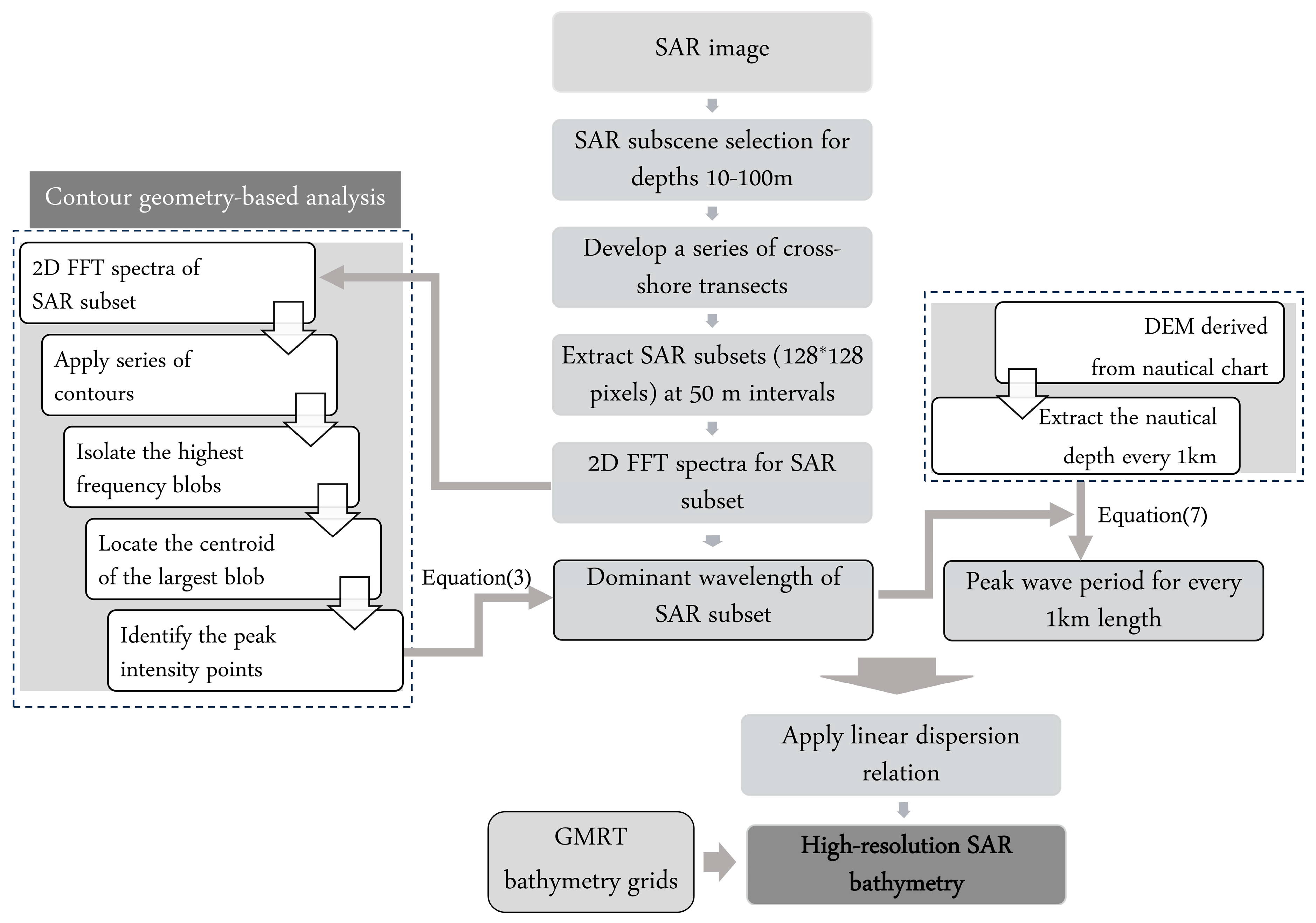
Fast Fourier transform (FFT) [20,21,24] is frequently used to analyze SAR datasets to estimate the wavelengths. FFT is a technique that decomposes a signal (image) in a special (e.g., spatial) domain into its constituent frequency components, enabling the identification of any regular periodicity in the input signal (image). Wavelet analysis is another alternative technique that analyzes the SAR subsets in different scales and angles, in which scales and angles correspond to the wavelength and wave direction, respectively [25]. From the peak values in all the scale-angle component images, the dominant wavelength and the direction are obtained [26]. A study by Ma et al. 2021 [26] provides an example of wavelet-based SAR bathymetry, in which wavelet resolution is varied by adjusting the size of the wavelet box and the scale resolution. Similarly, 2D-FFT is used to generate a directional image spectrum from which the dominant wavelength and its direction are acquired. These wave parameters can be identified by finding the peak location of the 2D spectrum [10,15]. Even though several studies adopted FFT for wavelength estimation, a thorough analysis procedure to determine peak frequency-intensity locations is lacking. This study attempts to address this by introducing a novel contour geometry-based wavelength-retrieval algorithm that enables automation and efficiency.

The all-weather and all-day imaging capacity of SAR has a significant advantage over other satellite sensors and has opened a new door to the SDB community. SAR nearshore bathymetry prediction is constantly improving, with many researchers exploring new methods and approaches to increase accuracy. Most SAR-based bathymetry or underwater topography studies incorporate estimating spectra-driven wave parameters using FFT outputs. Traditionally, the size of the FFT analysis cell dictates the final resolution of SAR bathymetry maps, which lies around 1 km per pixel or worse [20,27,28]. As a result, the ocean floors beyond 20 m in depth have so far only been mapped to a resolution of a few kilometers using SAR images, and these coarse resolutions are often inadequate for many applications, including habitat mapping, tsunami hazard evaluation, navigation, ocean circulation, and climate change studies [29]. This necessitates the development of new SDB methods delivering finer resolutions with high accuracy. The present study provides new insights into deriving high-resolution bathymetry, encompassing incremental strides in the field of FFT-based SAR bathymetry. In addition, this study has attempted to bridge the gap between different imaging domains of optical bathymetry and SAR bathymetry by generating high-resolution SAR bathymetry products in deeper nearshore areas that can facilitate more detailed underwater morphology maps of the entire nearshore region.

Until the launch of the Sentinel-1 satellites, SAR images were acquired only by commercial satellites, limiting their availability and flexibility, which is evidenced by the small number of studies on SAR bathymetry inversion. The Sentinel-1 constellation offers high-resolution, openly accessible SAR data that are acquired systematically and with long-term continuity. Therefore, they constitute a reliable and durable data source that can effectively be used to infer water depths in coastal waters at a minimal cost. The use of a time series of Sentinel-1 images has been investigated in a few recent studies [6,19], with reasonably improved results. Demonstrating the feasibility of SAR technology in retrieving bathymetry around different parts of the world remains a topic of increased interest, emphasizing varying degrees of improvements to the established algorithms.

In accordance with the emerging trend in SDB technology toward the development of automatic processes and robust methodologies, this study introduces an automated bathymetry extraction framework over extensive deep coastal water stretches, emphasizing novel wavelength and wave period-retrieval algorithms. The effectiveness of the proposed model was assessed using multiple SAR images for consistency. With these new additions to the FFT workflow, a more rigorous and efficient framework is proposed to generate high-accuracy and fine-scale bathymetric estimates from SAR.

2. Study Region and Dataset

Florida’s coastal region has one of the highest concentrations of coastal communities in the United States, and its nearshore coastal waters are the most valuable (more than USD 30 billion in revenue per year) with the highest recreational use. The eastern coast of Florida consists of a narrower continental shelf with gradual depth gradients (Figure 1). There is a critical need for seafloor maps in this part of Florida, and cost-effective technologies to rapidly assess seafloor changes would be highly beneficial to many commercial and academic communities, boosting the blue economy of the state. The long ocean swell waves from the North Atlantic exhibit a predominantly southbound wave direction in this part of Florida, with refraction leading to waves aligning with the shoreline as they approach the coast. The average significant wave height along this region varies from 0.9 m to 1.3 m, with minimum wave heights occurring during summer months (e.g., 0.59 m to 0.84 m) and maximum wave heights predominating during winter months (e.g., 1.1 m to 1.55 m [30]. The regional average wave periods lie in the range of 7 s to 9 s in this area [30].

The eastern Florida continental shelf contains a diversified region with various terrain types such as sand flats, ridge fields, coral reefs hummocky topography, etc., and geomorphological features like storm bars, bypass bars, and diabathic channels, etc., based on the geomorphological studies carried out by Fink et al. [31,32] along the Atlantic coast of Florida. Further, this area satisfies three of the most important traits of being able to apply the SAR bathymetry inversion using FFT methods. These characteristics include having a swell-wave regime, an extended nearshore region of depths below 100 m, and a negligible effect from currents (e.g., the current velocity is less than 0.05 m/s) [19]. The study site was divided into depth classes of 5–20 m, 20–40 m, 40–60 m, 60–80 m, and 80–100 m, as depicted in Figure 1.

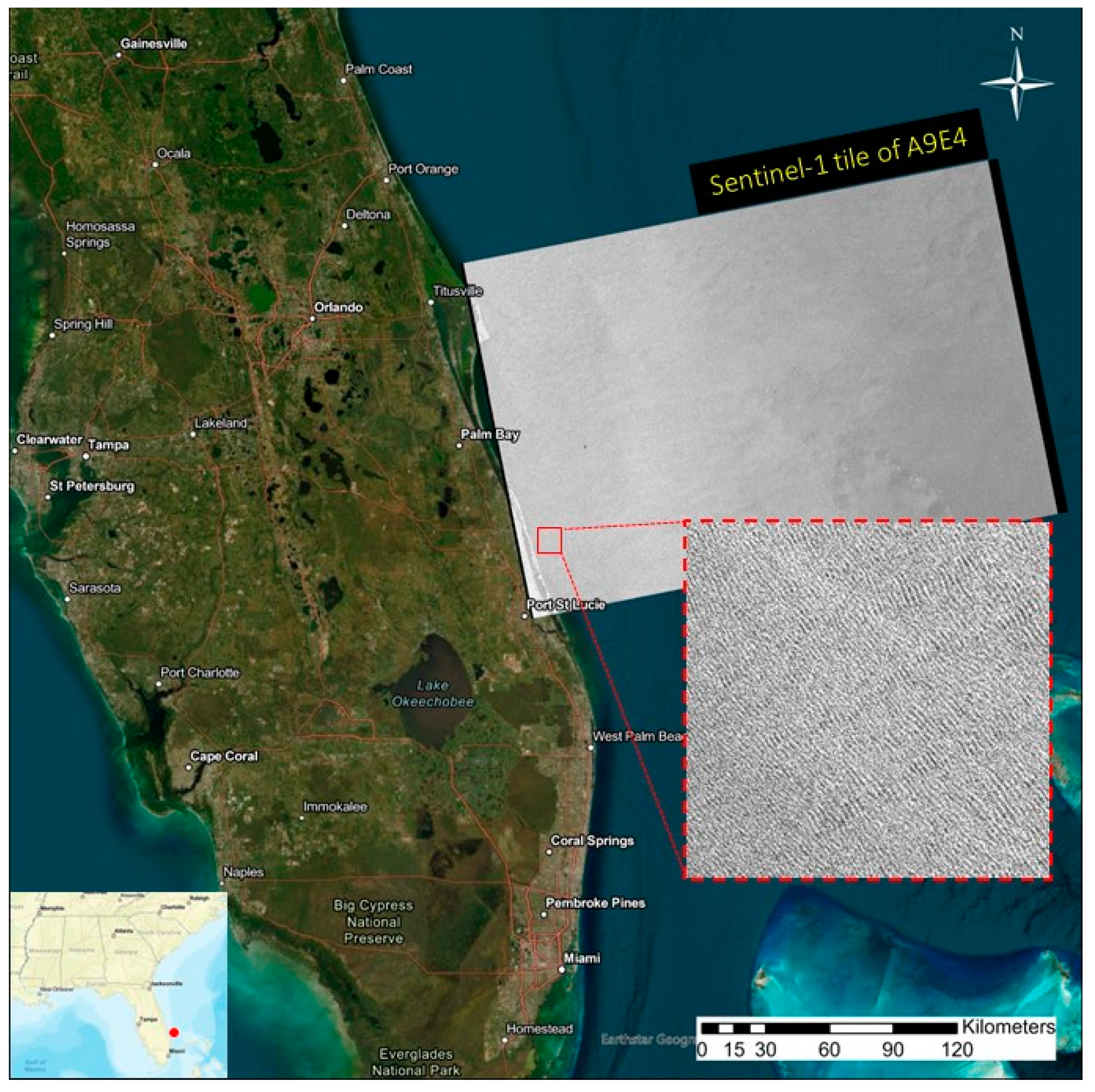
2.1. Sentinel-1 SAR Images

In the present study, Sentinel-1A, which was launched in 2014 and carries a C-band payload of 5.405 GHz, was used to gather SAR data to retrieve the bathymetry of the study region. From the available modes of data acquisition, an interferometric swath mode (IW) with a spatial pixel resolution of 10 m was used. The main challenge for the successful adaptation of SAR bathymetry is retrieving SAR images with visually identifiable wave patterns that can be attributed to radar image technology, as described in Section 3.1. The Sentinel-1 image tile with the identifier A9E4 was selected, which covers the eastern Florida region (Figure 2). The coastal sector between Wabasso Beach (northern boundary) and Jensen Beach (southern boundary) was used as the study site, which has an extended region of depths below 100 m. A boundary condition of depth of 100 m was set to define the wave shoaling region, which encompassed a total area of 3120 km² area bounded by a 70 km shoreline from one side.

The swell pattern visibility on SAR imagery is a constraining factor in selecting the best Sentinel-1 images for the analysis. Images with sea surfaces require distinct characteristics of surface waves to be able to correlate the wave behavior with the seafloor morphology [20]. Image selection was performed on the Sentinel Hub EO Browser using an AOI and VV-polarized image (decibel gamma0) preview as the filtering tool. A set of two images (

Table 1. Specifics of the selected two Sentinel-1 images of image A and image B.

Attribute	Image A	Image B
Acquisition Date and Time	18 November 2019, 23:20 UTC (Universal Time Coordinated)	10 November 2021, 23:21 UTC
Sensor Mode	IW (Interferometric Wide)	IW
Product Type and Resolution Class	GRDH (Ground-Range Detected, High Resolution)	GRDH
Processing Level	1 (Focused, Detected, Multi-Looked, Ground-Range Projected)	1
Spatial Resolution (m)	10	10
Pass	Descending	Descending
Polarization	Single VV (Vertical Transmit, Vertical Receive)	Single VV
Product Unique Identifier	A9E4	A9E4

) fulfilled these criteria, and their Level-1 Ground-Range Detected (GRD) products, which are multi-looked and projected to the ground range using an Earth ellipsoid model (WGS84), were downloaded from the Copernicus Open Access Hub.

2.2. Auxiliary Data

Two forms of auxiliary data that are openly accessible are used in this study. The nautical charts available in this area were used to acquire the reference depth data required for local wave period estimation. An Electronic Navigational Chart (ENC) corresponding to US3FL30M, downloaded from NOAA, was used for this purpose. This ENC is a geo-referenced NOAA nautical chart with a scale of 1:466,944 and is available in S-57 format (https://www.charts.noaa.gov (accessed on 4 August 2023)). The 000 file, which contains 3D vector data, was converted to a grid elevation model using Global Mapper v22. For validation purposes, Global Multi-Resolution Topography (GMRT) grid data were selected as the ground truth. GMRT synthesis is a multi-resolution compilation of edited multibeam sonar data gathered by various sources, which are processed and gridded by the Marine Geoscience Data System (MGDS) team and delivered as a single continuously updated global elevation dataset with a resolution of 100 m [33].

3. Methodology

3.1. SAR Ocean Imaging

Bragg waves provide the small-scale surface roughness required for the backscattering of the microwaves [34]. Thus, the presence of Bragg waves on the sea surface is a prerequisite for the wave features to become visible on radar images. The intensity of SAR backscatter from the ocean surface has a positive correlation with the ocean surface roughness. Bragg scattering constitutes the dominant backscattering mechanism for incidence angles(θ_i) between 20° and 60° [20]. The Bragg waves, which are in the order of SAR wavelengths, can be expressed by

$${\lambda }_B=0.5{\lambda }_r\sin {\theta }_i$$

(1)

where ${\lambda }_r$ is the radar wavelength and ${\lambda }_B$ is the sea surface wavelength.

The SAR imaging capability of the ocean waves is governed by three modulation mechanisms: tilt modulation, hydrodynamic modulation, and velocity brunching modulation. Out of these three, the velocity brunching is a non-linear mechanism that arises due to the motion of ocean surface waves relative to the direction of the SAR satellite [35]. The azimuth-traveling component of the orbital motion of the waves (parallel to satellite flight direction is the azimuth direction) enables SAR to image these waves through velocity brunching phenomena [19]. Based on this velocity brunching modulation, a threshold SAR wavelength called the azimuth cutoff wavelength can be defined as:

$$L_{min}=R\sqrt{H/V}$$

(2)

where $R$ is the slant range of the observed wave, $V$ is the SAR platform velocity, and $H$ is the significant wave height.

For SAR to image and detect the swell patterns of any azimuth traveling waves, their swell wavelengths need to be greater than this cutoff wavelength. This condition is one of the prerequisites to assume that the SAR imaged wavelengths are truly the original swell wavelengths [6] and can be identified as a major limiting factor of the observation of ocean waves by an SAR satellite [36]. Therefore, to perform an SAR-based analysis of shallow-intermediate coastal depths (which are characterized by shorter wavelengths), the $L_{min}$ needs to be as low as possible.

3.2. Bathymetry from Swell Waves

The two-dimensional FFT of an SAR subset of $N\times N$ pixel size gives a 2D image spectrum [37]. If the selected sub-image presents a sinusoidal-like dominant element, then its Fourier representation will depict a high peak of energy at the frequency of such a component [21]. The transformed image in the frequency domain needs to be analyzed to identify symmetrical sharp peaks on either side of the origin, from which the wavelength and wave direction of the dominant sea waves in each subscene are estimated.

After locating the sharp peaks on the transformed FFT representation, analytical relations are used to estimate the wavelength ($\lambda$) from the inverse of the distance separating the two peaks (Equation (3)), while the wave direction ($\theta$) is estimated from the orientation of the line connecting the two peaks (Equation (4)) [12].

$$\lambda =\frac{Pixel Size}{\sqrt{{\left(\frac{\mathsf{\Delta }x}{2M}\right)}^2+{\left(\frac{\mathsf{\Delta }y}{2N}\right)}^2}}$$

(3)

$$\theta =\arctan \frac{\mathsf{\Delta }y}{\mathsf{\Delta }x}$$

(4)

where $N$ is the number of rows of pixels, $M$ is the number of columns (for a square pixel $N$ = $M$), $\mathsf{\Delta }x$ is the number of columns between the two identified sharp peaks, and $\mathsf{\Delta }y$ is the respective difference in the number of rows.

Linear dispersion relation is used to calculate the bathymetry in moderately deep or shallow water. Derived from linear wave theory, the linear dispersion relation describes the swell-wave propagation and the relationship between the wavenumber, wave period, and wavelength. The shallow water depth ($h$) can be retrieved from the rearranged linear dispersion relation (Equation (5)) in which the two wave parameters, namely local wavelength ($\lambda$) and peak wave period ($T_p$), are needed [12].

$$h \left(\lambda , T_p\right)=\frac{\lambda }{2\pi }atanh\frac{2\pi \lambda }{g{T}_p{}^2}$$

(5)

3.3. Estimation of Wave Parameters

The two main maritime parameters required for the bathymetry prediction were retrieved locally using rigorous and repetitive analytical procedures.

3.3.1. Wavelength from FFT

The distance between two identical points on successive waves (e.g., crest to crest or trough to trough) is defined as the wavelength. Wavelength retrieval plays a vital role in predicting bathymetry in deeper nearshore coastal waters. Inaccuracies in wavelength retrieval lead to larger bathymetry deviations in deeper waters with longer waves than in shallower waters with shorter waves [27]. There are two main FFT methods exploited by recent studies, namely wave-tracing mode (transects along the wave propagation direction) and fixed-grid mode (standard gridded approach). In this study, due to the distinctive wave behavior with refraction within the study region, a wave-tracing approach is utilized. A total of forty cross-shore transects at equal intervals were generated along the 70 km shoreline of the study area. The transects were digitized perpendicular to the incoming wave crests imaged on the SAR. In most SAR studies, the SAR subsets and thus local wavelengths are provided for coarse, spatially non-overlapping grid cells. In contrast, the SAR subset generation in this study was performed overlappingly to provide spatially dense bathymetry to address the low resolution of bathymetry maps at these depths. SAR subsets of 128 × 128 pixels were extracted every 50 m along these transects and used to determine the dominant wavelengths. This was performed using the ArcPy library in ArcGIS Pro v2.7.1.

Two-dimensional FFT was applied on each extracted SAR subset along each transect. The FFT outputs demonstrate two clusters of high intensities located symmetrically on either side of the origin (Figure 3). However, it is not straightforward to identify the peak intensity in each cluster, as highlighted in Figure 3. It should be noted that the location of the peak intensity is our target variable, rather than the magnitude of the highest intensity. In analyzing these FFT plots, a robust method to consistently determine a representative point for the location of the frequency with the highest intensity is needed.

As a solution, a contour plot of pixel intensities was generated for the frequency domain representations. As a result, the FFT spectrum (Figure 4a) was divided into contour blobs (Figure 4b) highlighting the intensity hotpots in a more pronounced manner. This enables the high-intensity blobs on the FFT output to be isolated using an intensity threshold. For this purpose, the steepest contour levels in each FFT plot were used to identify the high-intensity blob (Figure 4c) while filtering out the lower-intensity regions. It should be noted that on a FFT spectrum, a cluster is defined as a group of adjacent pixels, while a blob is defined as an area bounded by a contour line.

Since there is no exact point of peak intensity but a cluster of pixels with high intensity in each isolated blob, it is imperative to determine an effective representative location for the sharpest peak. The geometric centroids of the high-intensity blobs on the FFT image spectrum were identified. The corresponding centroid on the closest blob is selected as the representative highest intensity. Using the symmetrical centroids on either side of the FFT origin, the wavelength for each SAR subset was estimated using Equation (3).

This algorithm is based on the contour geometry of the FFT subscene, which, in turn, is dependent on the wave structure imaged on the analyzed SAR subset. It provided an effective method to overcome the main hurdle in FFT workflow with regards to wavelength estimation, facilitating an automated workflow and improving the efficiency of the proposed method. MATLAB was used to perform the task of contour plot-driven dominant wavelength estimation. A summary of the workflow is depicted in Figure 5.

3.3.2. Peak Wave Period from Nautical Charts

The wave period can be described as the time for successive wave crests to pass a specific spatial point. The peak wave period ($T_p$) denotes the wave period associated with the most energetic waves in the wave spectrum at a specific point. The originating wind fields often offer the momentum to the swell-wave regimes to navigate through nearshore regions, varying the wave period locally. The minimum peak period threshold ($T_{min}$) describes the threshold that enables distinguishing the estimated swell wavelengths belonging to shallow or deep waters, which is computed using the deep-water linear dispersion relation [12]:

$$T_{min}=\sqrt{2\pi {\lambda }_{max}/g}$$

(6)

where ${\lambda }_{max}$ denotes the maximum detected wavelength.

The estimation of the peak wave period is a critical step in the water-depth derivation using linear wave theory. There are a few methods used in the recent literature to determine the peak wave period. Wiehle et al. [27] adopted an iterative approach to refine the peak-wave-period value using an initial water-depth value and the FFT technique. In Wiehle et al. [27], a range of peak-wave-period values was generated using tanh⁻¹($2\pi \lambda$/$g{T}^2$) < |1|, and corresponding depth values were estimated. The depth values yielded for each SAR subscene are compared against the reference depth, and a root-mean-square deviation (RMSD) analysis was performed to decide on the optimal peak wave period.

The in-situ measurements from wave buoys that are close to the observed area provide one such option for peak-wave-period determination although it is not always possible to have a wave buoy or historic data repository that can be queried even if wave buoys are located nearby. Another method requires an initial guess for the reference depth ($h_{ref})$, which can be extracted from nautical charts or freely available sources like GEBCO (available worldwide). The $T_p$ value can then be estimated using the linear dispersion relation, as in Equation (7), similar to [12,28].

$$T=\sqrt{2\pi \lambda /\left(gtanh\left(\frac{2\pi h_{ref}}{\lambda }\right)\right)}$$

(7)

In the present study, maintaining $T_p$ above the theoretical minimum $T_{min}$ indicated in Equation (6), it is estimated using the universally available nautical chart depths. This procedure improves the operational validity and facilitates the evaluation of the preciseness that can be replicated in regions without high-resolution bathymetry or even in remote coastal areas. To account for local wave regime conditions, $T_p$ values were calculated at 1 km intervals along each transect using Equation (7). The $T_p$ value is dependent upon both the depth and the wavelength value, which, in turn, describes the local wave regime at each location. The calculated $T_p$ value at a location is then used to derive the bathymetry within a 500 m proximity along the specific transect. This procedure was repeated for all 40 transects.

4. Results

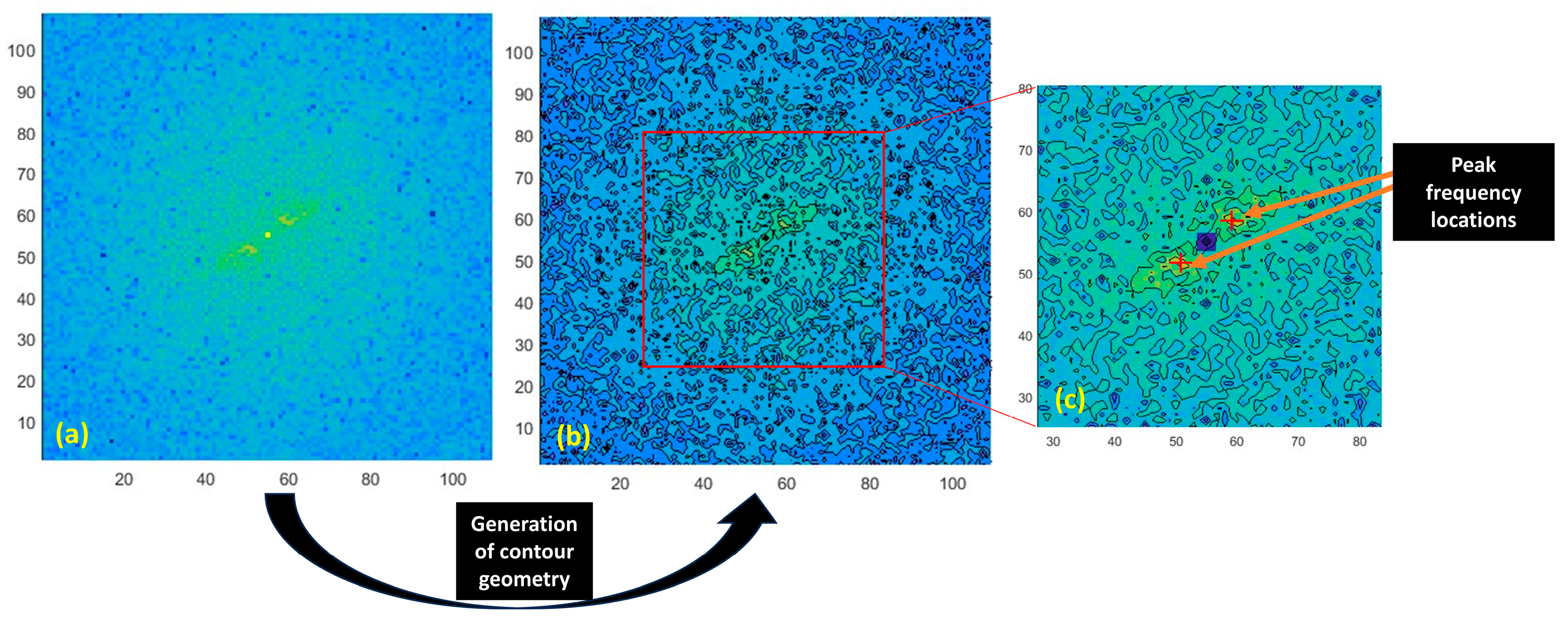
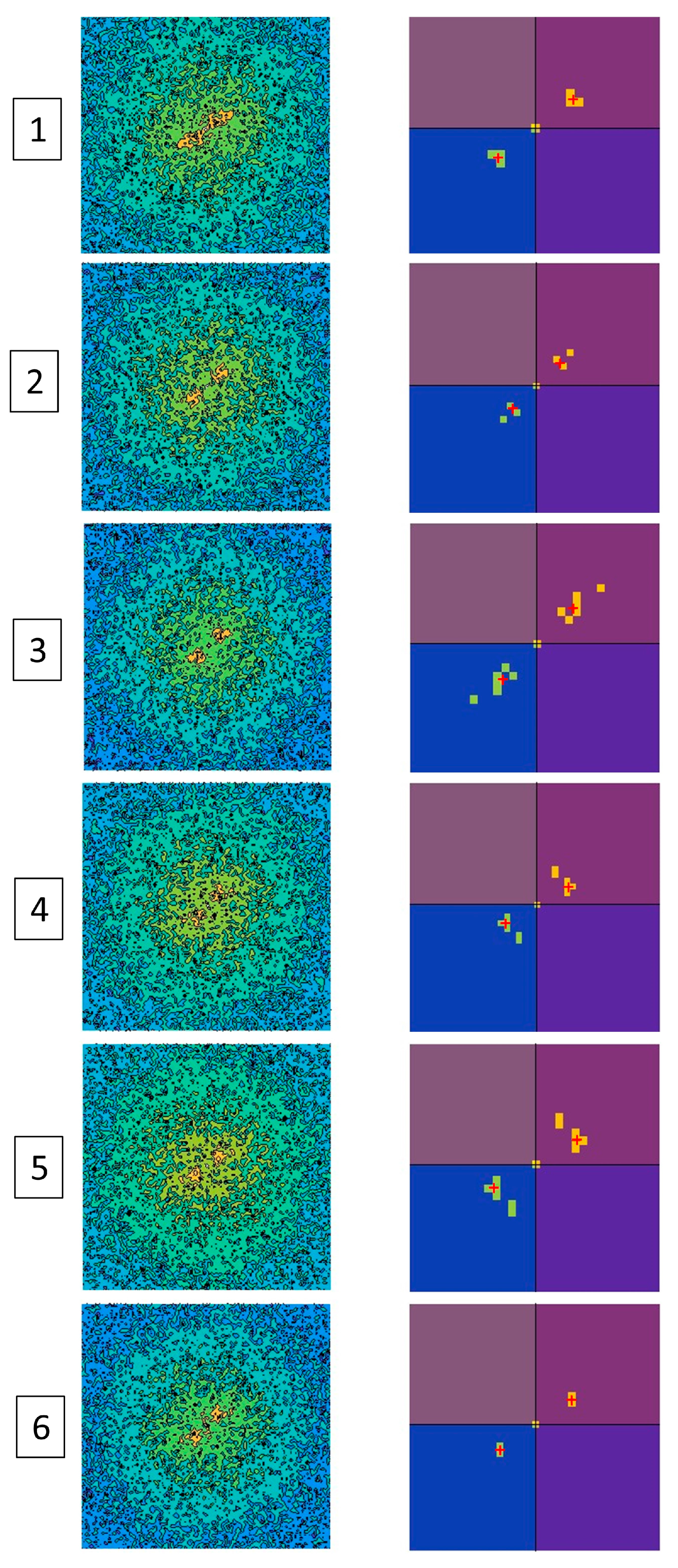
The wavelength-estimation procedure underwent rigorous testing and parameter optimization for the number of contour levels, the threshold value for isolating the high-intensity blobs, and the selection of the best centroid out of neighboring centroids. As a result, the optimal number of contour levels was determined to be 20. The threshold value for isolating the high-intensity blobs was found to be the value of the highest contour level. Finally, the best centroid out of neighboring centroids in each sector was determined to be the centroid attributed to the largest blob closer to the origin. It should be noted that the location of the highest intensity is our target variable, rather than the magnitude of the peak intensity. As depicted in Figure 6, the frequency contour plot generated for the FFT output yielded a representative value for the location of the peak intensity. The realization of the proposed approach in determining the accurate wavelengths enabled us to achieve better accuracy for depth prediction.

At some points in the spatial domain, a few calculated wavelength values revealed sudden unrealistic changes, differing significantly from surrounding values. To rectify the influence of these erroneous points, a moving mean wavelength value was adopted along each transect to reduce the effect of outliers. The proposed automated model for wavelength retrieval yielded results that are in line with the swell-wave regime with large wavelengths occurring in the open ocean, while shoaled and refracted shallow water waves generated modest wavelengths (Figure 7). This trend of descending wavelengths when moving from offshore to onshore is evident along all forty transects.

The wavelength and seafloor depth have a positive correlation. The gradual increments evident in the wavelength reflect this relationship with the underwater landscape when moving from shallow to deep waters. The bumps and anomalies that are present in the otherwise deepening seabed could be observed through the sudden dips and peaks of wavelength profiles (Figure 7).

While the estimation of wavelength is performed by the aforementioned method, the second parameter of the peak wave period is estimated using the nautical chart readings, which cover an extensive coastal water domain of 3120 square kilometers. The wave period in such a large coastal setting encompasses many swell-wave groups, and the wave period is given as a value range rather than a single value in many studies in the literature [38]. Accordingly, spatially attributed $T_p$ values could be more reliable and effective to suit the local swell-wave regime characteristics in such a large spatial extent, especially when our goal is to achieve high-resolution seafloor depth estimation. The estimated $T_p$ values lie in the range of 11–16 s when neglecting the shallowest region within which the dispersion relation does not hold. The wave buoy at Station 41114-Fort Pierce, FL, is the closest to the study site. Images A and B were captured at 2320 h on 18 November 2019 and 10 November 2021, respectively. From the National Data Buoy Center hosted by NOAA, Station 41114 records a dominant wave period (DPD) (the period with the maximum wave energy) of 13.33 s and 14.12 s at 2330 h on respective days. These wave buoy readings fall within the estimated $T_p$ value range, reflecting the credibility of the developed wave period-estimation procedure. Further, the effect of $T_p$ on the bathymetry estimation is quantified and included in Section 5.1.

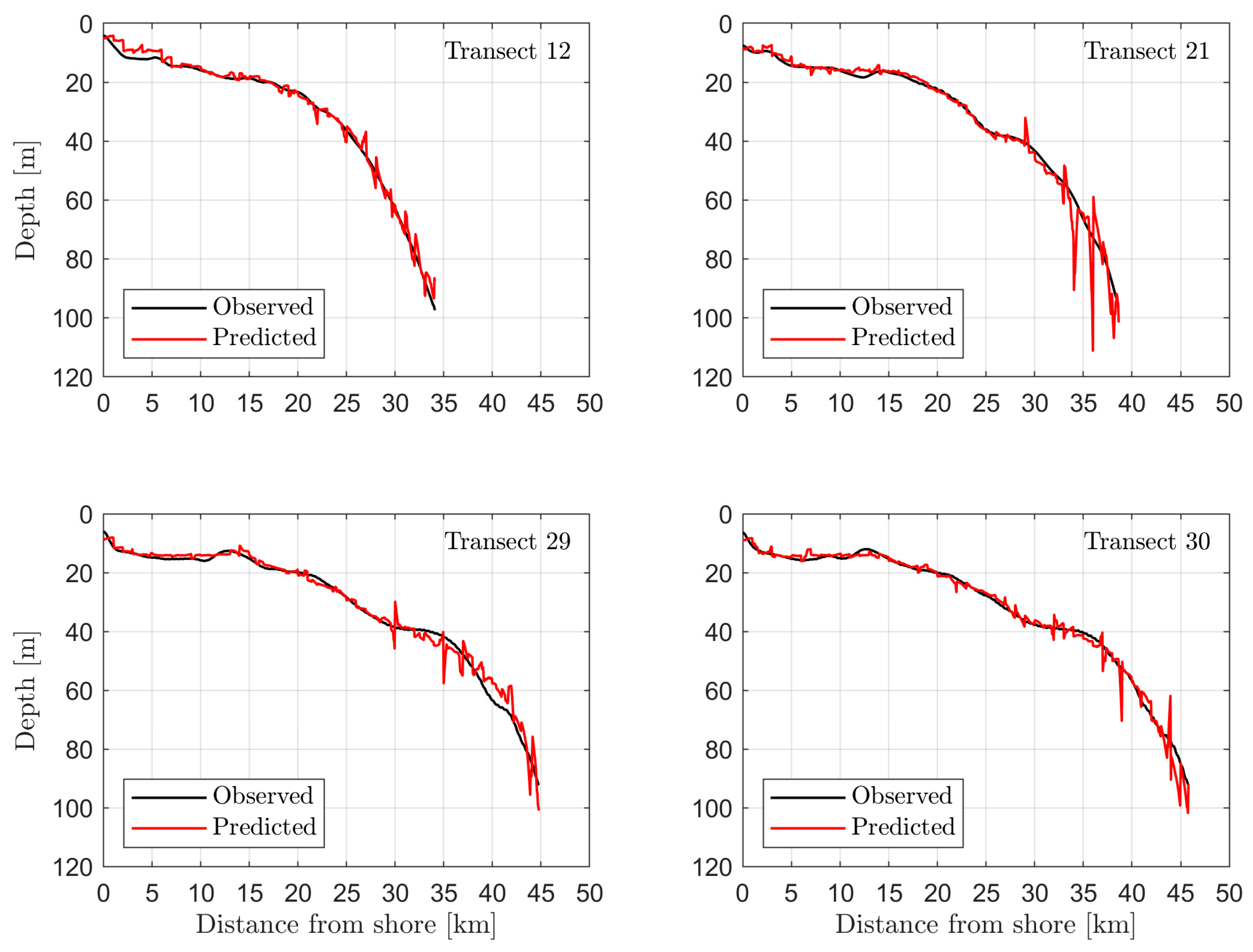
The depth values were deduced using the adjusted linear dispersion relation of Equation (5) and compared against the GMRT profile. The performance of the model is then evaluated along each transect by measuring the root-mean-square error (RMSE) and relative percentage error. The depth profiles acquired using SAR images A and B along four selected transects that represent the entire depth domain of the study area are illustrated in Figure 8 and Figure 9, respectively. The overall inferred underwater topography agrees well with the reference GMRT data. The analysis of SAR-predicted bathymetry for depths below 60 m indicates that the local variations in depth are reproduced well. It is also evident from Figure 8 and Figure 9 that the depth prediction along both steep (transect 12) and gradually varied (transects 29 and 30) underwater terrains remains consistently accurate. The figures show that the accuracy of depth prediction decreases with increasing depth.

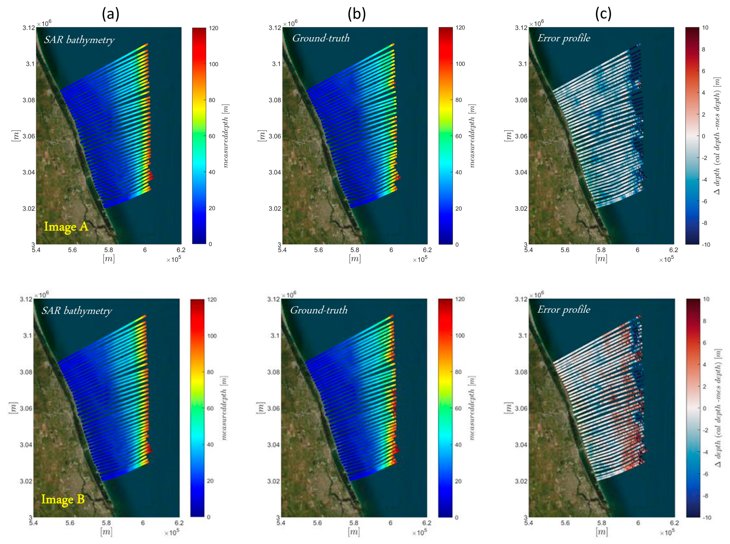
The estimated SAR bathymetry and the error distribution, in comparison with reference GMRT data for both SAR images A and B, are depicted in Figure 10. It should be noted that the inferred bathymetry from SAR data within the depth domain of 10–100 m is in good agreement with the GMRT depth grids. The trend of the seabed deepening with the distance from the shoreline is captured, which aligns with different depth classes witnessed within the study region. Figure 10 and

Table 2. Error metrics corresponding to each depth class for images A and B.

Depth Class (m)	Image A		Image B
	RMSE (m)	Relative Error (%)	RMSE (m)	Relative Error (%)
5–20	1.90	10.40	1.99	10.89
20–40	1.56	4.47	1.72	4.78
40–60	2.40	3.56	3.09	4.32
60–80	9.67	10.61	10.20	11.08

also indicate that, overall, image A produces better accuracy than image B.

Each transect runs through the entire nearshore region, covering depths of 5 m to 100 m. To better evaluate model performance at different depth domains, a quantitative analysis of the results for the depth classes introduced in Section 2 is presented in Table 2. The RMSE and relative percentage error are used to measure the performance of the developed method. It is evident that the RMSE values reflect consistently high accuracy up to the 60 m depth limit, beyond which the accuracy decreases with increasing depth. This also reveals that the relative error percentages are low (0–5%) for both the mid-depth classes of 20–40 m and 40–60 m. Consequently, the depth range of 20–60 m could be interpreted as the most optimal region for SAR bathymetry in the study area.

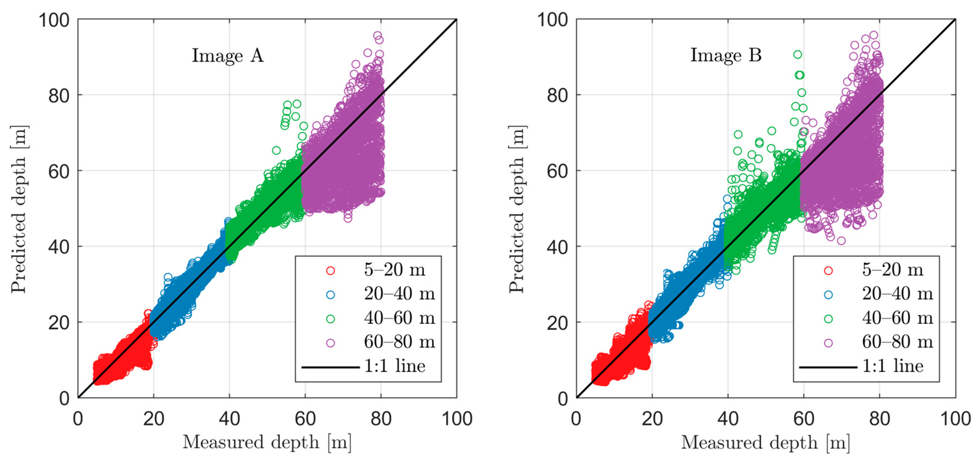
Figure 11 illustrates scatter plots of predicted and observed water depths for all 31,200 points along all the transects. The points were color-coded according to the depth classes introduced in Table 2. The coefficients of determination $R^2$ are 0.96 and 0.95 for image A and image B, respectively, indicating a strong correlation. An underprediction tendency is evident across all four depth classes, while the prediction accuracy has been reduced substantially beyond the depth of 60 m. Overall, considering the large sample of data points, the results are consistently accurate for these deep coastal regions.

5. Discussion

Only a limited number of studies have addressed SAR bathymetry estimation so far, and the majority of them used the FFT spectrum analysis. An FFT-based SAR bathymetry inversion study by Pleskachevsky A. et al. in 2011 [12] achieved 15% accuracy for depths of 20–60 m. A study by Brusch S. et al. in 2011 [20], using TERRASAR-X data, yielded 5 m errors for 72% of the validation entries. Wiehle S. et al. in 2019 [27] yielded RMSD values of 6.5 m, 6.7 m, and 7.7 m for water depths of 10–20 m,20–30 m, and 30–40 m, respectively, using TerraSAR-X images and an FFT approach. More recently, Huang L. et al. in 2022 [28] yielded an MAE of 2.9 m and an ${\mathit{R}}^2$ of 0.93 using multi-source SAR images, finding that SAR resolution plays a more vital role than its polarization mode in bathymetry derivation. The accuracy levels obtained in this study are in line with or better than those achieved in the abovementioned previous SAR studies. Moreover, the best resolution for current SAR bathymetry obtained using FFT analysis is 320 m [6] and 500 m [21]. Thus, the improved resolution of 50 m along transect lines within these challenging deep coastal areas can be identified as a big stride in SAR bathymetry generation.

The present study serves as the first to investigate a high sampling rate like a 50 m interval for FFT-derived wavelength extraction and led to high-resolution bathymetry retrieval. The derivation of the predominant wavelength in successive SAR subsets is facilitated by an automatic peak intensity identification algorithm. It should be noted that the high-intensity blob geometries exhibit distinctive shapes on FFT outputs descendant from consecutive SAR cells, thus leading to the most fitting estimate for the dominant wavelength. The robustness of this technique is tested through its application over a vast depth range that spans from 5 m to 80 m. This strengthens the adaptive characteristic of the proposed contour geometry-driven wavelength-retrieval algorithm, which offers more flexibility and scalability to SAR bathymetry inversion in deeper nearshore coastal regions.

The contour geometry-based wavelength-retrieval algorithm applied to the FFT has improved both the efficiency and accuracy of the SAR-based bathymetry-estimation procedure. Most FFT-based SAR bathymetry studies provide an insufficient analysis of the peak location derivation in determining the dominant wavelength. Pereira et al. [21] developed an algorithm that provides a scale of the dominance of the identified wave based on the sharpness of the peaks on the FFT domain. From the results of this study, due to the proximity of the peak intensity pixels, they tend to develop an inter-connected geometry that could be isolated to find the best corresponding point of the peak intensity. The proposed approach associating the contour geometry within the FFT output is a novel technique that addresses the lack of clarity and insufficient depth of analysis in the determination of peak frequency-intensity locations, which leads to more robust wavelength derivation.

The proposed methodology is suited to deriving the wavelengths and peak wave periods of local swell-wave regimes in nearshore coastal settings. The coastal depths at which the swell waves interact with the seabed would provide the optimal region for the method to deliver better depth prediction. The depth inversion was best at the interval of 20–60 m, consistently producing highly accurate bathymetry prediction across two SAR images. The accuracy of the depth prediction, expressed as a relative accuracy, was found to be relatively low in the shallowest and the deepest depth classes in Table 2. These two depth domains coincide with the wave-breaking zone and deep sea, respectively, within which the linear wave theory does not hold anymore. When the propagating waves encounter the shallow areas, they rear up, resulting in wave breaking. From the point of wave breaking, the linearity in wave theory does not hold, thus leading to inferior results for depths between 5 and 15 m. However, the RMSEs of 1.90 m (image A) and 1.99 m (image B) are reasonable for a 5–20 m depth and are in line with SDB studies focused on optical methods. Therefore, a fusion of optical and SAR can be recommended for the 5–20 m depth range, as many studies suggest an extinction depth for optical SDB of 10–20 m [2,5].

Overall, this study emphasizes several advantages over the existing literature on SAR bathymetry. The most prominent is the automated workflow to generate high-resolution bathymetry beyond 20 m deep coastal areas. Further, this study provides an effective peak intensity-locating algorithm to enable efficient wavelength derivation. The proposed peak-wave-period algorithm, which provides more depth-appropriate estimates, would be more effective in a large coastal setting compared to the existing methods of using a single value or a value range for ${\mathit{T}}_{\mathit{p}}$.

This study can be further improved to establish the feasible depth domain with SAR technology more precisely. Bian X. et al. 2020 [19] show that there is a minimum and maximum detectable depth range for SAR that, in turn, is a function of the type of the SAR signal (L band [19], S band [39], C band [26], X band [20], etc.), maximum detectable swell wavelength, and swell-wave period. However, there is a potential to improve these findings using the sub-surface variations detected by high-spatial-resolution bathymetry maps facilitated by this study. Wave breaking marks the end of the shoaling zone within the nearshore region, which can be digitized precisely. This boundary line further provides the onshore limit of SAR bathymetry, thus informing the boundaries of the surf zone within which the wave action is expected to be most turbulent and dynamic and thus difficult to be predicted by SDB in general. This could also be replicated in demarcating the offshore shoaling zone in a more precise manner. Furthermore, these findings will aid in the numerical modeling of cross-shore sediment dynamics within the nearshore region [40].

The work in the present study only used openly accessible Sentinel-1 images and nautical chart data; thus, the bathymetry generation can be reproduced in other regions of the world with minimal cost. The results reveal that the proposed method is capable of generating high-resolution bathymetry with high accuracy and consistency over a large and diversified coastal region. Additionally, the automation approach developed in this study would certainly be the first step in improving the resolution and accuracy levels of FFT-SAR bathymetry. Further, it would pave the way forward for scalable SAR bathymetry, with minor adjustments to suit specific study areas.

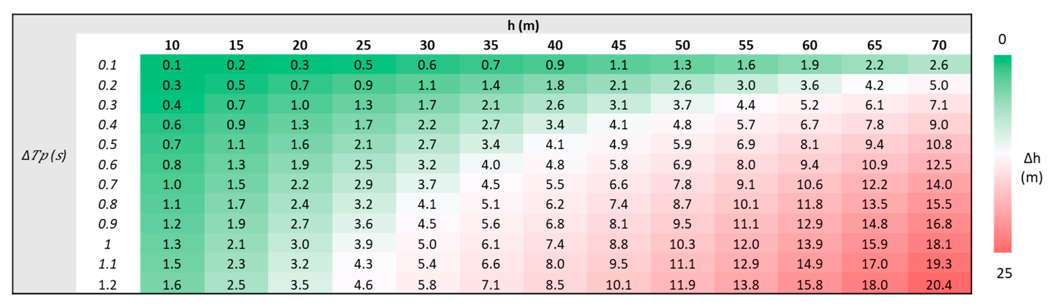
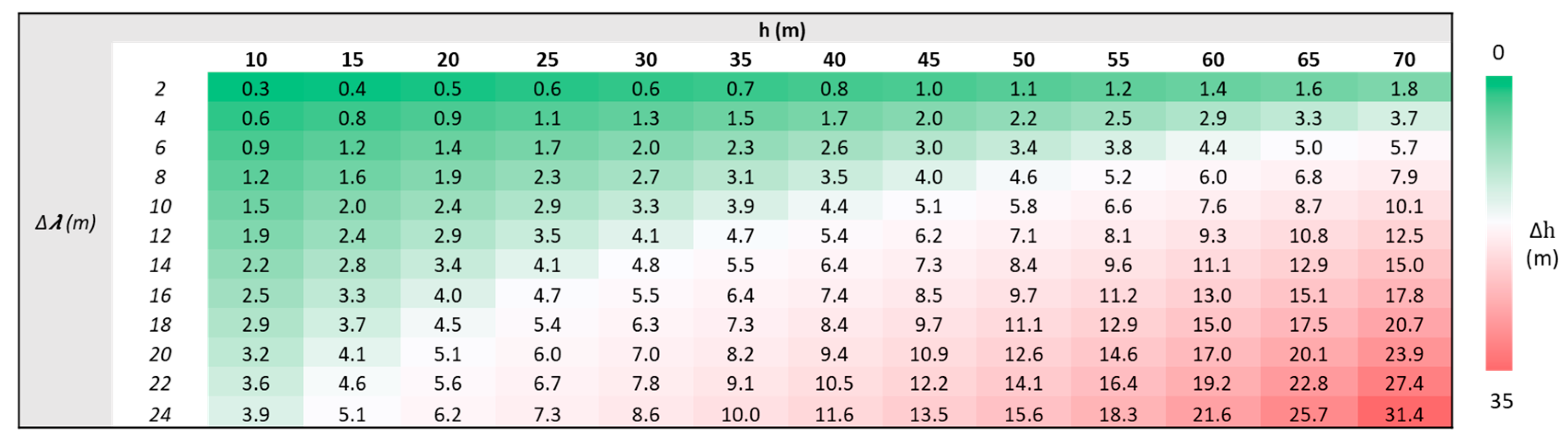
5.1. Sensitivity Analysis

A sensitivity analysis is performed to evaluate the proposed model’s overall uncertainty. Sensitivities associated with both the peak wave period and wavelength are estimated using a combination of typical depth and wavelength combinations. An average peak wave period of 15 s is used throughout, while linear dispersion relation-based wavelengths were calculated for each depth. The results are highlighted in Figure 12 (${\mathit{T}}_{\mathit{p}}$ sensitivity) and Figure 13 (λ sensitivity). In each depth column in Figure 12, the depth change ($\mathit{\Delta }\mathit{h}$) was calculated for incremental ${\mathit{T}}_{\mathit{p}}$, keeping the wavelength constant. Similarly, in Figure 13, $\mathit{\Delta }\mathit{h}$ was calculated for incremental $\lambda$, keeping the peak wave period constant. The horizontal axis provides the depth, and the vertical axis corresponds to the incremental change of ${\mathit{T}}_{\mathit{p}}$ or $\lambda$, while the sensitivity of the initial depth $\left(\mathit{\Delta }\mathit{h}\right)$ is color-coded within each cell. Figure 12 and Figure 13 reveal that the sensitivity to the ${\mathit{T}}_{\mathit{p}}$ or $\lambda$ adjustments increases with the water depth. For an uncertainty of 4% (0.6 s) in ${\mathit{T}}_{\mathit{p}}$ deviation, a water depth of 26.8 m (−3.2 m) is obtained for a 30 m depth. Thus, a 4% error in wave period is translated to a 10.6% error in water-depth calculation at a 30 m depth. In contrast, a 4% error in wave period is translated to a much larger 15.6% error in water-depth estimation at a 60 m depth. Therefore, the uncertainty arising from the wave period increases with increasing water depths. Accordingly, an uncertainty of 4% (10 m) in $\lambda$ deviations results in 11.0% and 12.6% water-depth errors at 30 m and 60 m depths, respectively. The findings of this sensitivity analysis are in agreement with Wiehle et al. [27]. According to Wiehle et al. [27], the RMSE of depth estimation increases by 2.4 m if the period is varied by + or −0.5 s from the optimal ${\mathit{T}}_{\mathit{p}}$ value, citing it to be a crucial step for retrieving accurate bathymetry estimates. Bian et al. [19] found that the water depths derived from linear dispersion relation are most sensitive to the peak wave period and moderately sensitive to the wavelength. Subsequently, further studies to estimate the effect of SAR image quality, wave parameters, and sea conditions on SAR bathymetry are suggested.

The quality of SAR images is the main factor that influences the prediction capacity of the proposed model. The model developed does not inherently detect the non-sea state signals and SAR image distortions produced by short wind waves or breaking waves. Such an SAR algorithm was utilized in [41], which determines the marine parameters of the very short waves that are not visible in the SAR signal. The addition of such elements would facilitate accommodating lower-quality SAR images in the bathymetry-estimation process. It should be also noted that the selected two images, which were acquired in two different years (assuming the seabed morphology in these deeper regions has not changed drastically) allowed for the evaluation of the internal consistency of the proposed depth-retrieval algorithm. The difference in the accuracy levels of depth predictions between images A and B (Figure 10 and Table 2) can be attributed to different noise levels of the two images and to the data acquisition discrepancies between the SAR data and the reference data.

The selection of SAR images requires a more methodical approach to identify the images with a swell-wave field propagating along the flight direction of the SAR sensor. In theory, the velocity brunching phenomenon causes the azimuth traveling waves to be smeared, making them of limited value for SAR bathymetry purposes [18]. This image selection process can be improved by incorporating environmental factors such as wave heights, wind speed, and surface current velocity during SAR data acquisition. A program to detect swells imaged by SAR as long and regular features exhibiting bright and dark alternating stripes would be a viable solution.

Sentinel-1 (5.4 GHz) data are transforming the field of coastal sciences with unprecedented volumes of openly accessible spatial information. The proposed automated approach, which only utilized Sentinel-1, could easily be extended to other SAR data sources with differing radar frequencies, such as ENVISAT ASAR (5.3 GHz), ALOS PALSAR (1.27 GHz), GF-3 (5.4 GHz), RADARSAT-1 (5.3 GHz), etc. NISAR, with its new dual-frequency radar imaging system, is another promising SAR data source that will be available, with an expected launch in 2024. Smaller radar frequencies facilitate a more distinct contrast on SAR images that will aid in wave pattern distinction, while large radar frequencies produce a stronger backscatter intensity of the sea surface [28]. Further, the size of the FFT cell is a crucial element for dominant wavelength extraction that would lead to more depth-appropriate predictions, which could be a topic for future studies. It is also recommended to assess the versatility of the proposed method in different marine environments with various wave conditions and geomorphological settings.

6. Conclusions

The openly accessible Sentinel-1 SAR images have the potential to produce consistent bathymetric products with high spatial detail and high resolution in optically non-viable, deeper nearshore coastal waters. The depth retrieval of these challenging deep regions was only possible with expensive multibeam echo-sounders (MBES), making them scarce and less repetitive. The generation of SAR-based bathymetry in this study allowed for repeatable water-depth estimation in challenging water depths at fine spatial resolutions. The SAR-based SDB model developed in this study utilized an automated wave-parameter and depth-retrieval approach applied over an extensive coastal region. These promising bathymetric frameworks, which are low-cost and scalable, are paving the way to advancing marine research and planning, climate change understanding, coastal restoration, the management and monitoring of coastal ecosystems, and navigation worldwide. Moreover, with SAR-based SDB producing consistent predictions in much deeper coastal depths with improved resolution, it can substantially improve change detection and benthic habitat monitoring.