Intelligent Environment-Adaptive GNSS/INS Integrated Positioning with Factor Graph Optimization

Abstract

Global navigation satellite systems (GNSSs) applied to intelligent transport systems in urban areas suffer from multipath and non-line-of-sight (NLOS) effects due to the signal reflections from high-rise buildings, which seriously degrade the accuracy and reliability of vehicles in real-time applications. Accordingly, the integration between GNSS and inertial navigation systems (INSs) could be utilized to improve positioning performance. However, the fixed GNSS solution uncertainty of the conventional integration method cannot determine the fluctuating GNSS reliability in fast-changing urban environments. This weakness becomes solvable using a deep learning model for sensing the ambient environment intelligently, and it can be further mitigated using factor graph optimization (FGO), which is capable of generating robust solutions based on historical data. This paper mainly develops the adaptive GNSS/INS loosely coupled system on FGO, along with the fixed-gain Kalman filter (KF) and adaptive KF (AKF) being taken as comparisons. The adaptation is aided by a convolutional neural network (CNN), and the feasibility is verified using data from different grades of receivers. Compared with the integration using fixed-gain KF, the proposed adaptive FGO (AFGO) maintains the 100% positioning availability and reduces the overall 2D positioning error by up to 70% in the aspects of both root mean square error (RMSE) and standard deviation (STD).

1. Introduction

Global navigation satellite systems (GNSSs) are a widely recognized navigation technology that has been applied in various fields, including robotics, the military, and agriculture. Intelligent transport systems (ITSs) are one of the most popular research areas due to the prosperity of autonomous vehicles. However, the system performance highly depends on positioning accuracy. In urban canyons, GNSS signals are susceptible to multipath and non-line-of-sight (NLOS) effects due to the reflection and blockage of signals from high-rise buildings [1]. The multipath effect may cause meters of positioning error, while an NLOS signal can seriously deteriorate the GNSS positioning accuracy to errors of a hundred meters [2,3].

Numerous research has been proposed to enhance the accuracy and reliability of GNSS positioning results. The 3D-mapping-aided (3DMA) GNSS approach is one of the popular methods applied in urban areas. Researchers [4,5] employed a 3D building model incorporated with the ray tracing technique to predict the transmission path of the GNSS signal and correct the NLOS delay. Lee et al. [6] developed an algorithm that matches images taken by a fisheye camera with skymasks generated by 3DMA to decide the position and heading of the fisheye image. However, this method requires an up-to-date 3D building model and strong computational power to simulate the path and process the image. Another popular approach is multi-sensor fusion. The development of GNSSs, inertial navigation systems (INSs), and light detection and ranging (Lidar)-integrated systems have enhanced the positioning continuity and accuracy during GNSS outage periods and under challenging environments [7,8]. Wan et al. [9] adaptively fused GNSS, Lidar, inertial measurement unit (IMU), and real-time kinematic (RTK) sensors according to an uncertainty estimation algorithm to prevent system failures in various scenes. Cao et al. [10] proposed a tightly coupled GNSS–visual–inertial fusion system to cope with challenging environments for positioning. However, incorporating multiple sensors results in increased cost, which forms a barrier to integration into commercial products, whereas GNSS/INS integration is more economical and widely applicable in the industry. Enhancing the positioning accuracy of GNSS/INS integration using various algorithms has attracted researchers’ interest. The coupling methods can be divided into loosely coupled (LC), tightly coupled (TC), and ultra-tightly coupled (UTC) depending on the type of GNSS data used to perform integration. LC integration utilizes the position information of GNSS receivers, while TC integration uses the raw GNSS measurements such as pseudo-range and Doppler observables [11,12]. In UTC integration, in-phase (I) and quadrature-phase (Q) components of the signal are directly fed into the filter [13]. However, it requires adjustment on receiver architectures, which limits its applicability with general equipment. The traditional KF method and its extensions, such as extended Kalman filter (EKF), unscented Kalman filter (UKF), and cubature Kalman Filter (CKF), are the most common integration algorithms. The effectiveness and robustness of KF-based algorithm have been verified by several studies [14,15,16,17,18,19,20,21]. Kim et al. [17] employed EKF to integrate linearized correlator outputs and INS measurements. Nevertheless, EKF might cause large errors during the linearization process. Instead of approximating non-linear functions by a Taylor series expansion, UKF adopts probability distribution to represent the non-linearity [18]. A derivative UKF of TC integration was proposed by Hu et al. [19] to achieve at least a second-order accuracy of the Taylor series. CKF features more accurate state estimation using the cubature technique [20], and the research work by Liu et al. [21] proved that CKF further reduces the positioning error and computational time compared with UKF. Particle filter (PF) is another filtering technique that utilizes importance sampling to draw particles from the selected importance density and calculate the corresponding weight of each particle. Unlike the KF-based algorithms, this method can handle non-linear systems and non-Gaussian noise [22]. Researchers usually incorporate PF with other techniques in GNSS/INS integration. For example, the unscented PF proposed by Seo et al. combines the benefits from UKF and PF and shows superior noise reduction capability [23]. However, the intrinsic disadvantage of PF, such as being more receptive to measurement noise in resampling [24] and significantly rising computational load when the number of particles increases [25], make it less favorable than KF.

Approximating non-linear functions may still cause errors, and the optimization procedure is applied to the current state without considering the wide range of historical data. To further improve the performance of state estimation, the use of factor graph optimization (FGO) has attracted researchers’ attention. It is a novel integration method that maximizes a posterior probability of system states [26]. All sensor measurements are considered as related state variables (i.e., factors) of the factor graph, which are used to construct the function of maximization problems. This technique is widely used in a variety of fields such as simultaneous localization and mapping (SLAM), artificial intelligence, and wireless networking [15,27]. Studies have also shown that FGO can remarkably enhance the positioning performance in GNSS/INS integration compared with the KF-based methods [28]. A recent work proposed by Wen et al. [11] showed that FGO outperforms EKF in terms of positioning accuracy in both LC and TC integration. Chang et al. [29] incorporated GNSS/INS/LiDAR-SLAM with FGO, and the results showed that FGO achieves a lower than 1-meter root mean square error (RMSE) in urban areas. Li et al. [30] suggested the auto-regressive integrated moving average (ARIMA) auxiliary model to supply GNSS data during the GNSS outage period, and the integration results conducted by factor graph algorithm have a better performance compared with EKF. Zeng et al. [31] suggested a multi-sensor fusion algorithm based on FGO, which fuses information from the GNSS receiver, barometric altimeter, magnetometer, optic flow sensor, and sonar sensor. These research studies show that FGO has great potential in increasing positioning accuracy. In the aspect of data processing, rather than considering only the previous epoch like KF, FGO utilizes all historical data to improve the accuracy of estimation [32], which increases the resistance against outliers and enhances estimation accuracy. However, the fact that FGO considers all historical information and uses more complex optimization techniques leads to higher computational complexity, which becomes an obstacle to the application in real time. Another advantage of FGO is that the graphical model has a straightforward architecture and therefore enables a more flexible “plug and play” integration of GNSS and INS information.

Despite the great advantage brought by various GNSS/INS integration algorithms, the measurement reliability of different GNSS receivers may still be challenging to determine properly. Fast-changing urban environments can significantly deteriorate GNSS positioning and result in fluctuating solution quality; therefore, the GNSS solution uncertainty can hardly be regarded as fixed. In contrast, adaptively changing the value of uncertainty can largely improve the fused solution quality in the urban environment [33]. This conception comes with different practices of adaptive KF (AKF). Wu et al. [15] proposed an adaptive EKF model to adjust the covariance matrix of EKF based on dilution of precision (DOP). Zhang and Hsu [16] employed machine learning to determine the noise covariances of KF. Such environment-dependent functionality can also be enabled by the deep learning approach, which has been proven effective in solving different types of problems and applied in many research of GNSS field over the recent years [6,34,35,36]. CNN, as one of the most popular deep learning algorithms, is inspired by human brain neurons and has the significant advantage of capturing complex patterns and spatial information through functions such as filtering and pooling. Moreover, for the same dimension of inputs, CNN contains a fewer total number of trainable parameters than the conventional fully connected neural network, thus appearing to be less prone to overfitting [37,38].

Motivated by strengths brought from the FGO algorithm and CNN, the proposed AFGO approach first extracts some features from GNSS measurements and then predicts the GNSS solution uncertainty used in the adaptive GNSS/INS integration with the trained CNN model. Moreover, it is considered that the carrier phase measurement is popular in precise positioning, but its performance can be significantly degraded in urban areas due to cycle slips and the poor measurement quality of consumer-grade devices [39]. Thus, this study was focused on using the code measurement rather than the carrier phase measurement for positioning. The contribution of this paper is fourfold: (1) we developed an adaptive GNSS/INS integrated positioning algorithm implemented by MATLAB based on the FGO architecture to achieve better accuracy and robustness; (2) we employed deep learning to predict the GNSS solution uncertainty during its integration with INS; (3) we assessed and compared the performance of conventional KF and FGO with the open-source large-scale datasets, UrbanNav [40] in terms of different grades of receivers; and (4) we validated the feasibility of the proposed algorithm using the preceding large-scale datasets with different environments (i.e., different urbanization levels) and receiver grades.

The rest of this paper is structured as follows: Section 2 demonstrates the mechanisms of GNSS/INS coupling methods, while Section 3 will discuss how the adaptive functions operate in multi-sensor coupling. The validation of the proposed algorithm will be presented using experiments in Section 4, along with a further evaluation of results in Section 5. Section 6 will finally itemize some limitations of current work, summarize this study, and propose prospective research areas.

2. System Architecture of Adaptive GNSS/INS Integration by FGO

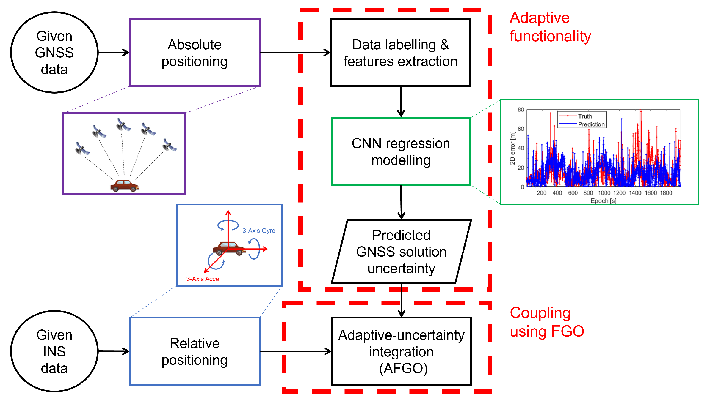
The proposed adaptive FGO (AFGO) approach integrates two sensors’ inputs, including the absolute positioning from GNSS and relative positioning from INS. Figure 1 essentially shows the workflow, which contains scenarios of both the adaptive and fixed integration based on the settings of GNSS solution uncertainty. As depicted in the workflow of Figure 1, the adaptive uncertainty comes from the prediction of the trained CNN regression model, whose input features are extracted from GNSS. Combined with the FGO-based algorithm, the adaptive uncertainty AFGO is carried out for analysis.

2.1. Basic Parameters about GNSS, INS, and the State Vector

At epoch t, the system state vector ${\mathit{S}}_{\mathit{t}}$ depicted in Equation (1) contains the information of positions ${\mathit{X}}_{\mathit{t}}^{\mathit{ecef}}$, orientation ${\mathsf{\Phi }}_{\mathit{t}}^{\mathit{body}}$, velocity ${\mathit{V}}_{\mathit{t}}^{\mathit{ecef}}$, and INS bias ${\mathit{B}}_{\mathit{t},\mathit{INS}}^{\mathit{body}}$, whose specifications [11,16] are displayed as:

$${\mathit{S}}_{\mathit{t}}={\left[{\mathit{X}}_{\mathit{t}}^{\mathit{ecef}},{\mathsf{\Phi }}_{\mathit{t}}^{\mathit{body}},{\mathit{V}}_{\mathit{t}}^{\mathit{ecef}},{\mathit{B}}_{\mathit{t},\mathit{INS}}^{\mathit{body}}\right]}^T$$

(1)

$${\mathit{X}}_{\mathit{t}}^{\mathit{ecef}}=\left[x_t^{ecef},y_t^{ecef},z_t^{ecef}\right]$$

(2)

$${\mathsf{\Phi }}_{\mathit{t}}^{\mathit{body}}=\left[{\psi }_t^{body},{\theta }_t^{body},{\varphi }_t^{body}\right]$$

(3)

$${\mathit{V}}_{\mathit{t}}^{\mathit{ecef}}=\left[{v_x}_t^{ecef},{v_y}_t^{ecef},{v_z}_t^{ecef}\right]$$

(4)

$${\mathit{B}}_{\mathit{t},\mathit{INS}}^{\mathit{body}}=\left[{\mathit{B}}_{\mathit{t},\mathit{f}}^{\mathit{body}},{\mathit{B}}_{\mathit{t},\omega }^{\mathit{body}}\right]=\left[{b_N}_{t,acc}^{body},{b_E}_{t,acc}^{body},{b_D}_{t,acc}^{body},{b_N}_{t,gyro}^{body},{b_E}_{t,gyro}^{body},{b_D}_{t,gyro}^{body}\right]$$

(5)

where “ecef” denotes the global coordinates based on the Earth’s center and “body” means the North-East-Down (NED) frame based on the body centroid. The raw sensor data from both the accelerometer and gyroscope, denoted by ${\mathit{A}}_{\mathit{t},\mathit{INS}}^{\mathit{body}}$, are shown as the following:

$${\mathit{A}}_{\mathit{t},\mathit{INS}}^{\mathit{body}}=\left[{\mathit{A}}_{\mathit{t},\mathit{f}}^{\mathit{body}},{\mathit{A}}_{\mathit{t},\omega }^{\mathit{body}}\right]=\left[{A_N}_{t,acc}^{body},{A_E}_{t,acc}^{body},{A_D}_{t,acc}^{body},{A_N}_{t,gyro}^{body},{A_E}_{t,gyro}^{body},{A_D}_{t,gyro}^{body}\right]$$

(6)

Therefore, the INS measurement input ${\mathit{U}}_{\mathit{t}}$ at epoch t (originated from previous epoch $t-1$) can be expressed as:

$${\mathit{U}}_{\mathit{t}}={\mathit{A}}_{\mathit{t}-\mathbf{1},\mathit{INS}}^{\mathit{ecef}}={\mathit{T}}_{\mathit{GB}}\left({\mathit{A}}_{\mathit{t}-\mathbf{1},\mathit{INS}}^{\mathit{body}}-{\mathit{B}}_{\mathit{t}-\mathbf{1},\mathit{INS}}^{\mathit{body}}\right)$$

(7)

where ${\mathit{T}}_{\mathit{GB}}$ is a transformation matrix from body frame to global frame, and ${\mathit{A}}_{\mathit{t}-\mathbf{1},\mathit{INS}}^{\mathit{body}}$ and ${\mathit{B}}_{\mathit{t}-\mathbf{1},\mathit{INS}}^{\mathit{body}}$ represent raw sensor data and bias from the previous epoch, respectively. Moreover, the absolute position measurement from GNSS, ${\mathit{Z}}_{\mathit{t},\mathit{GNSS}}$, is shown as:

$${\mathit{Z}}_{\mathit{t},\mathit{GNSS}}={\left[x_{t,GNSS}^{ecef},y_{t,GNSS}^{ecef},z_{t,GNSS}^{ecef}\right]}^T$$

(8)

2.2. Kalman Filter

For each epoch t, the basic KF formulation [24] mainly consists of an INS state transition in Equation (9) and GNSS measurement update in Equation (12). Additionally, the error covariance matrix ${\mathit{P}}_{\mathit{t}}$ in Equation (10) introduces the system noise covariance ${\mathit{Q}}_{\mathit{t}}$, and the GNSS measurement in Equation (11) is assumed to satisfy Gaussian distribution with the measurement noise covariance matrix ${\mathit{R}}_{\mathit{t}}$, which represents exactly the GNSS solution uncertainty to be tuned in this study. The process noise, given GNSS information, can be calculated by Equation (13).

$$\begin{array}{c}{\widehat{\mathit{S}}}_{\mathit{t}}^{\mathbf{-}}={\mathit{F}}_{\mathit{t}\mathbf{-}\mathbf{1}}{\widehat{\mathit{S}}}_{\mathit{t}\mathbf{-}\mathbf{1}}^{+}+{\mathit{U}}_{\mathit{t}\mathbf{-}\mathbf{1}}\end{array}$$

(9)

$$\begin{array}{c}{\widehat{\mathit{P}}}_{\mathit{t}}^{\mathbf{-}}={\mathit{F}}_{\mathit{t}\mathbf{-}\mathbf{1}}{\widehat{\mathit{P}}}_{\mathit{t}\mathbf{-}\mathbf{1}}^{+}{\mathit{F}}_{\mathit{t}\mathbf{-}\mathbf{1}}^T+{\mathit{Q}}_{\mathit{t}\mathbf{-}\mathbf{1}}\end{array}$$

(10)

$$\begin{array}{c}{\mathit{Z}}_{\mathit{t}\mathbf{,}\mathit{GNSS}}={\mathit{H}}_{\mathit{t}}{\widehat{\mathit{S}}}_{\mathit{t}}^{\mathbf{-}}+\mathcal{N}\left(0,{\mathit{R}}_{\mathit{t}}\right)\end{array}$$

(11)

$$\begin{array}{c}{\widehat{\mathit{S}}}_{\mathit{t}}^{\mathbf{+}}={\widehat{\mathit{S}}}_{\mathit{t}}^{\mathbf{-}}+{\mathit{K}}_{\mathit{t}}\left({\mathit{Z}}_{\mathit{t}\mathbf{,}\mathit{GNSS}}-{\mathit{H}}_{\mathit{t}}{\widehat{\mathit{S}}}_{\mathit{t}}^{\mathbf{-}}\right)\end{array}$$

(12)

$$\begin{array}{c}{\widehat{\mathit{P}}}_{\mathit{t}}^{+}=\left(1-{\mathit{K}}_{\mathit{t}}{\mathit{H}}_{\mathit{t}}\right){\widehat{\mathit{P}}}_{\mathit{t}}^{-}\end{array}$$

(13)

(“+” and “−” means before and after GNSS measurement update, while “$\widehat{}$” highlights estimated variables. ${\mathit{F}}_{\mathit{t}\mathbf{-}\mathbf{1}}$ and ${\mathit{H}}_{\mathit{t}}$ stand for the state transition matrix and measurement matrix, respectively. ${\mathit{K}}_{\mathit{t}}$ is the Kalman gain, calculated using ${\mathit{H}}_{\mathit{t}}$, ${\widehat{\mathit{P}}}_{\mathit{t}}^{\mathbf{-}}$, and ${\mathit{R}}_{\mathit{t}}$).

Because this study focuses on the post-processing of the positioning solutions, a Rauch–Tung–Striebel (RTS) smoother [24,41] has been employed after the filter to improve the smoothness of trajectories. The backward process has been expressed in Equation (14)–(16), where the overscript “$\mathit{s}$” stands for the smoothed variables.

$$\begin{array}{c}{\mathit{K}}_{\mathit{t}}^{\mathit{s}}={\widehat{\mathit{P}}}_{\mathit{t}}^{\mathbf{+}}{\mathit{F}}_{\mathit{t}}^{\mathit{T}}{\left({\widehat{\mathit{P}}}_{\mathit{t}\mathbf{+}\mathbf{1}}^{\mathbf{-}}\right)}^{-1}\end{array}$$

(14)

$$\begin{array}{c}{\widehat{\mathit{S}}}_{\mathit{t}}^{\mathit{s}}={\widehat{\mathit{S}}}_{\mathit{t}}^{\mathbf{+}}+{\mathit{K}}_{\mathit{t}}^{\mathit{s}}\left({\widehat{\mathit{S}}}_{\mathit{t}\mathbf{+}\mathbf{1}}^{\mathit{s}}-{\widehat{\mathit{S}}}_{\mathit{t}\mathbf{+}\mathbf{1}}^{\mathbf{-}}\right)\end{array}$$

(15)

$$\begin{array}{c}{\widehat{\mathit{P}}}_{\mathit{t}}^{\mathit{s}}={\widehat{\mathit{P}}}_{\mathit{t}}^{\mathbf{+}}+{\mathit{K}}_{\mathit{t}}^{\mathit{s}}\left({\widehat{\mathit{P}}}_{\mathit{t}\mathbf{+}\mathbf{1}}^{\mathit{s}}-{\widehat{\mathit{P}}}_{\mathit{t}\mathbf{+}\mathbf{1}}^{\mathbf{-}}\right){\left({\mathit{K}}_{\mathit{t}}^{\mathit{s}}\right)}^T\end{array}$$

(16)

2.3. Factor Graph Optimization

In the factor graph, GNSS and INS data participate in the coupling as connected factors (i.e., $f^{GNSS}$ and $f^{INS}$) of the undirected structure, as depicted in Figure 2. The example graph shows the state vector $\mathit{S}$ from initial epoch 1 to the final epoch n, with an example section at epoch t being specially displayed.

In the loosely coupled structure, the GNSS factor represents the measurement constraints between the estimated states and the measurements obtained from GNSS. At epoch t, GNSS factor ${\mathit{f}}_{\mathit{t}\mathbf{,}\mathit{GNSS}}$ comes from the position measurement updated by the receiver with a Gaussian noise $N(0,{\mathsf{\Sigma }}_{\mathit{GNSS}})$ assumption. With the GNSS observation function denoted as $h^{GNSS}(·)$ and GNSS solution represented by ${\mathit{Z}}_{\mathit{t}\mathbf{,}\mathit{GNSS}}$, the GNSS factor can be modeled as:

$${\mathit{f}}_{\mathit{t}\mathbf{,}\mathit{GNSS}}={\mathit{Z}}_{\mathit{t}\mathbf{,}\mathit{GNSS}}=h^{GNSS}\left({\mathit{S}}_{\mathit{t}}\right)+N(0,{\mathsf{\Sigma }}_{\mathit{GNSS}})$$

(17)

where ${\mathsf{\Sigma }}_{\mathit{GNSS}}$ exactly represents the GNSS solution uncertainty and can be tuned to achieve both fixed and adaptive coupling. This is comparable with the measurement covariance ${\mathit{R}}_{\mathit{t}}$ in KF, and the detailed settings will be specified in Section 4.1. Moreover, the discrepancy between the measurement and the prediction constitutes the error function of the GNSS factor:

$$\left|\right|{\mathit{e}}_{\mathit{t},\mathit{GNSS}}{\left|\right|}_{{\mathsf{\Sigma }}_{GNSS}}^2=\left|\right|{\mathit{Z}}_{\mathit{t}\mathbf{,}\mathit{GNSS}}-h^{GNSS}\left({\mathit{S}}_{\mathit{t}}\right){\left|\right|}_{{\mathsf{\Sigma }}_{GNSS}}^2$$

(18)

Similar to the GNSS factor, the INS factor demonstrates the relationship between the states $\mathit{S}$ and INS inputs $\mathit{U}$. It models the motion and enables tracking on the object’s movement at all epochs, even when the GNSS signal is temporarily unavailable. Mathematically, the states ${\mathit{S}}_{\mathit{t}}$ at current epoch t is obtained based on the states ${\mathit{S}}_{\mathit{t}\mathbf{-}\mathbf{1}}$ and INS measurements ${\mathit{U}}_{\mathit{t}\mathbf{-}\mathbf{1}}$, which contain the processed accelerometer and gyroscope measurements in global coordinates at the previous epoch $t-1$. The INS factor ${\mathit{f}}_{\mathit{t}\mathbf{,}\mathit{INS}}$ is defined as:

$${\mathit{f}}_{\mathit{t}\mathbf{,}\mathit{INS}}={\mathit{S}}_{\mathit{t}}=h^{INS}({\mathit{S}}_{\mathit{t}\mathbf{-}\mathbf{1}},{\mathit{U}}_{\mathit{t}\mathbf{-}\mathbf{1}})+N(0,{\mathsf{\Sigma }}_{\mathit{INS}})$$

(19)

where $N(0,{\mathsf{\Sigma }}_{\mathit{INS}})$ denotes the assumed Gaussian noise model with zero mean and noise covariance of ${\mathsf{\Sigma }}_{\mathit{INS}}$ and $h^{INS}(·)$ is the INS observation function. Correspondingly, the error function is given as:

$$\left|\right|{\mathit{e}}_{\mathit{t}\mathbf{,}\mathit{INS}}{\left|\right|}_{{\mathsf{\Sigma }}_{INS}}^2=\left|\right|{\mathit{S}}_{\mathit{t}}-h^{INS}({\mathit{S}}_{\mathit{t}\mathbf{-}\mathbf{1}},{\mathit{U}}_{\mathit{t}\mathbf{-}\mathbf{1}}){\left|\right|}_{{\mathsf{\Sigma }}_{INS}}^2$$

(20)

Combining the above, the FGO algorithm is designed to maximize the posterior probability of the system states given the GNSS and INS information, as shown in the equation:

$$\widehat{\mathit{S}}=\underset{\mathit{S}}{argmax}P\left(\mathit{S}\right|\mathit{Z},\mathit{U})$$

(21)

where $\mathit{S}$ is the set of state vectors, $\mathit{Z}$ is the set of GNSS solutions throughout all of the epochs, and $\mathit{U}$ is the set of INS inputs, respectively. Such an objective function can further be transformed to minimize the summation of error functions of both the GNSS and INS factors [11]:

$$\widehat{\mathit{S}}=\underset{\mathit{S}}{argmin}\sum _t\left(\right||{\mathit{e}}_{\mathit{t}\mathbf{,}\mathit{GNSS}}{\left|\right|}_{{\mathsf{\Sigma }}_{GNSS}}^2+\left|\right|{\mathit{e}}_{\mathit{t},\mathit{INS}}{\left|\right|}_{{\mathsf{\Sigma }}_{INS}}^2).$$

(22)

At each epoch, FGO estimates the state by conducting optimization (i.e., Equation (22)) iteratively according to the information from all historical epochs from the first epoch to the current epoch t. Meanwhile, KF only employs the INS propagation from epoch $t-1$ and the GNSS measurement at the current epoch t for estimation. With more historical information being considered in state estimation, FGO is proven to outperform KF in terms of accuracy and smoothness for the positioning solutions [11].

3. Adaptive GNSS Uncertainty Estimation by CNN

This section will mainly discuss the selected features in deep learning, the settings of the proposed CNN structures, and the mechanisms used to tune the GNSS solution uncertainty adaptively. This uncertainty requires adjustment of the GNSS solution noise covariance (${\mathsf{\Sigma }}_{\mathit{GNSS}}$) in Equation (17). The purpose of adaptation is to help improve the positioning accuracy of GNSS/INS integration compared with the methods with fixed solution uncertainty. In each second during the selected path, the truth 2D positioning error is obtained by comparing between the GNSS receiver’s solution and the ground truth position.

3.1. Features Related to GNSS Measurement Quality

During each available epoch, the eight proposed features that are discussed in the following will be extracted and then utilized as the inputs for the subsequent CNN model.

• Feature 1: Ratio of number of received satellite signals to the total number of available satellite signals
  The ephemeris data obtained from reference stations provides the PRN codes of all existing satellites in the sky. However, the received satellite number is always lower due to the blockage of GNSS signals by buildings. Therefore, the ratio of the number of received satellite signals to the total number of satellites in ephemeris data can indicate the obstruction level from buildings (i.e., the measurement quality).
• Feature 2: Mean elevation angles of satellites
  Research [42] has shown that when the elevation angle of a transmitter is lower than 15 degrees, 97% of the signals are blocked by the buildings in an urban environment. Signals are less likely to be blocked or reflected by buildings with high elevation angles, thus proving the mean elevation angle to be a critical feature for filtering NLOS signals.
• Feature 3 and 4: Mean and standard deviation of carrier-to-noise Ratio $C/N_0$
  $C/N_0$ represents the received signal strength, which is largely attenuated by reflection and blockage. A higher value of mean $C/N_0$ indicates less likelihood of an NLOS signal and thus better positioning performance. Given that the standard deviation shows the outlier signal, both the average and standard deviation of $C/N_0$ among the satellites could be adopted as features to identify the signal quality in each epoch.
• Feature 5 and 6: Mean and standard deviation of pseudo-range residuals
  A pseudo-range residual is used to provide information about the fitness of the least squares method [43], and a smaller pseudo-range residual reveals higher consistency between the measurement and the estimated positioning results. The pseudo-range residual ($ϵ$) is defined as the differences between the estimated pseudo-range ($\widehat{\rho }$) and the measured pseudo-range ($\rho$). The equation is:

  $$ϵ=\rho -\widehat{\rho }=\rho -G\widehat{x}$$

  (23)

  where G is a matrix consisting of the unit vector along LOS from user to satellites and $\widehat{x}$ is the converged state vector of users calculated by least squares estimation:

  $$\widehat{x}={\left(G^{T}G\right)}^{-1}{G}^T\rho$$

  (24)
• Feature 7 and 8: Mean and standard deviation of pseudo-range rate consistency
  Pseudo-range rate consistency is defined as the difference between the delta pseudo-range and the product of the pseudo-range rate and a unit time. Its mean and standard deviation can reflect the positioning performance of the receiver. The equation of pseudo-range rate consistency ($\delta$) is written as:

  $$\delta =\mid \Delta {\rho }_t^i-{\dot{\rho }}^i·\Delta t\mid$$

  (25)
  Delta pseudo-range is the difference of the pseudo-range between two epochs, and it is measured through the code tracking loop. The equation is expressed as:

  $$\Delta {\rho }_t^i={\rho }_t^i-{\rho }_{t-1}^i$$

  (26)
  The pseudo-range rate is computed using the Doppler shift as:

  $${\dot{\rho }}^i=-\frac{c}{f_{L1}}·f_{Doppler}^i$$

  where c is speed of light, $f_{L1}$ is the GPS L1 band frequency (1575.42 MHz), and $f_{Doppler}^i$ is the Doppler frequency obtained by the carrier tracking loop.

3.2. Positioning Error Prediction by CNN

Given the proposed eight features, the CNN model further outputs prediction ($P_{CNN}$) of the GNSS solution uncertainty. Figure 3 exhibits the overview of the whole structure. Specifically, the first convolutional layer receives the input feature in dimension of $8\times 1\times 1$ and filters it with 64 kernels in the size of $2\times 1$ with unit stride. After a MaxPooling layer is applied, the second convolutional layer repeats the settings of the first one, and the data are further max pooled by 64 (size $2\times 1$) kernels. This network utilizes the activation function rectified linear unit (ReLU) to guarantee non-negative feature values, and batch normalization and regularization are also applied to speed up the convergence [44]. Finally, followed by the $64\times 1$ fully connected neural network, the model outputs the predicted uncertainty through a regression layer. The rationale of using a convolutional layer lies in its ability to extract local features, which can further constitute more complex patterns, and the MaxPooling layer is adopted to reduce dimensions of the feature map and improve the network’s robustness to variations and noise of input data while keeping the most essential information inside. The regression layer enables the CNN to generate continuous value prediction, which coincides with the expectation on continuous outputs of 2D positioning errors.

As for the training data preparation, different datasets holding the extracted features are combined together sequentially epoch-by-epoch for shuffling after normalization on the feature values. Such normalization is also applied on the testing dataset when making predictions to guarantee that training and testing datasets are processed in the same way. It is worth mentioning that, strictly speaking, the inputs of this model are not images but a 1D array with GNSS feature values. The main idea of using CNN falls on its advantages, including exploring the correlation across different features and the higher-level efficiency of parameter usage through weight sharing to prevent overfitting, as mentioned in the Section 1. The training samples are the eight features extracted from the GNSS dataset and the label is the 2D error of the receiver positioning results with respect to the ground truth. The loss using the mean square error (MSE) method gives:

$$Loss=\frac{1}{R}{\mathsf{\Sigma }}_{i=1}^R{(y_i-P_{CNN,i})}^2$$

(27)

where R is the number of samples, $y_i$ indicates target output, and $P_{CNN,i}$ is the predicted output at ith sample. The learning objective is to determine the coefficients and biases in the neural network that can minimize the loss. The above CNN model will generate regression results that represent the estimated GNSS 2D positioning error, which also indicates the solution uncertainty in this study.

3.3. Uncertainty Adaptation

If GNSS 2D positioning solutions are not available, the INS measurement still propagates the receiver’s location. When having GNSS information, the algorithm employs loose coupling between GNSS and INS data. Unlike the fixed integration, which uses the same uncertainty value throughout all the integration epochs, adaptive integration applies different uncertainty in different epochs. It is noted that two kinds of extreme uncertainty are designed during this process. “Max uncertainty” performs as the upper bound used when extremely large pseudo-range rate consistency measurements exist. It is embodied in epochs with GNSS positioning whilst without valid CNN prediction because of the abnormal pseudo-range rate consistency (i.e., extreme values occur in Feature 7 and 8). In contrast, the “Min uncertainty” is assumed to be the lower limit for predictions, and any predicted uncertainty below this threshold is adjusted to the value of “Min uncertainty”. Both “Max uncertainty” and “Min uncertainty” are user-defined fixed values and vary according to different types of receivers. Apart from the extreme cases, all other epochs take the corresponding GNSS uncertainty based on CNN predictions, where the estimated 2D positioning error is considered equivalent to the GNSS uncertainty. The logic of adaptive uncertainty adjustment can be shown in the flow chart Figure 4 below, where $P_{CNN}$ denotes the CNN-predicted uncertainty. Along with the fixed uncertainty, parameters in adaptive integration are set differently across the receiver type, which will further be specified in the experimental part.

4. Performance Assessment and Validation

4.1. Experiment Setup

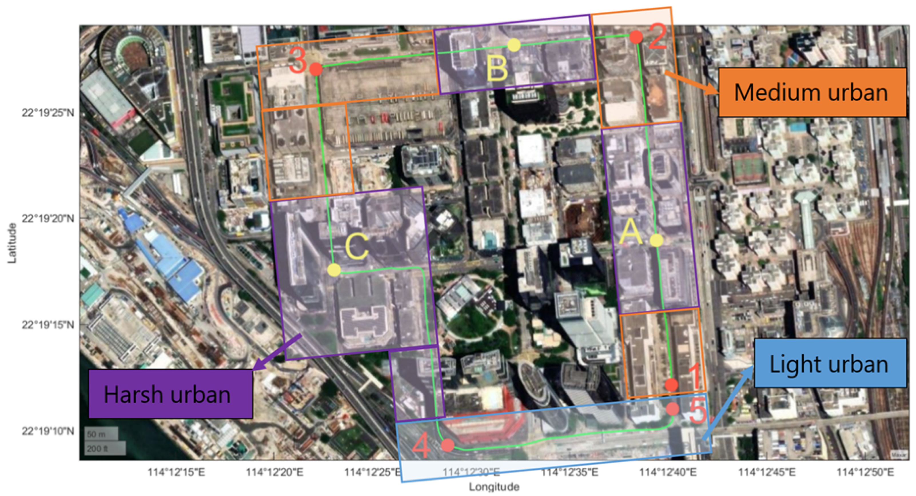
GPS and Beidou system data provided in the “UrbanNav” dataset are adopted in this study [40]. The Tsim Sha Tsui and Whampoa subsets are chosen as training data for deep learning, while another GNSS dataset from Kowloon Bay (depicted in Figure 5) with similar collection procedures is used as testing data and to validate the GNSS/INS integration. Especially, data from three commercial GNSS receivers, including U-Blox F9P, Xiaomi 8, and NovAtel Flexpak6 (noted as U-Blox, Xiaomi, and NovAtel later in this paper), are considered and utilized as the representatives of different level receivers. Additionally, a separate ground truth trajectory is given by NovAtel SPAN-CPT after inertial explorer (IE) post-processing for reference. As for the solution uncertainty parameters of each receiver, fixed uncertainty and min uncertainty are set based on the typical positioning performance of the receivers or data-processing experience. Based on that, max uncertainty is chosen at a value higher than two times the fixed uncertainty, indicating a situation of extremely large uncertainty. Details on such settings are presented in

Table 1. GNSS solution uncertainty settings.

Parameters	U-Blox	Xiaomi	NovAtel
Fixed uncertainty [m]	30	60	20
Max uncertainty [m]	65	130	45
Min uncertainty [m]	1.5	4	1

.

Apart from the GNSS receivers, the Xsens MTi-10 device and the smartphone built-in IMU device are chosen as the sensors that provide INS data for this study. The Allan Variance method [45] showcases the characteristics of the noise process and is used for IMU error analysis. It is applied in this study to obtain the INS bias and noise parameters for both the accelerometer and gyroscope [46], as summarized in

Table 2. INS noise and bias parameters.

Parameters	Value
Gyroscope noise term [rad2]	$2.5\times {10}^{-5}$
Gyroscope bias term [rad2/${\mathrm{s}}^2$]	$4\times {10}^{-11}$
Accelerometer noise term [${\mathrm{m}}^2/{\mathrm{s}}^2$]	$6.4\times {10}^{-5}$
Accelerometer bias term [${\mathrm{m}}^2/{\mathrm{s}}^4$]	$1\times {10}^{-5}$

.

This study analyses an almost completely end-to-end car trajectory. The whole duration is 920 s, but different receivers might have a different total number of available GNSS epochs. As depicted in Figure 5, four sections, with the labels and estimated durations 1–2 (1–255 s), 2–3 (256–605 s), 3–4 (606–770 s), and 4–5 (771–920 s), constitute the whole trajectory in an anticlockwise manner. Section 1–2 has tall buildings on both sides, while section 4–5 has one side with tall buildings and another side with an open-sky environment. Similar surroundings happen in section 2–3 and 3–4, where buildings are on both sides with less density than section 1–2. Points A, B, and C denote junctions where the car stops for some time, and they happen roughly in the time periods 110–130, 290–350, and 630–730 (in second), respectively. Additionally, the 920 s trajectory passes through various typical urban scenarios for positioning. Figure 5 highlights three types of urban environments: (1) light urban: region with quasi-open-sky environment or with open-sky view on one side of the street; (2) medium urban: region surrounded by buildings with height of less than 40 m; (3) harsh urban: region surrounded by buildings taller than 40 m or with streets less than 10 m in width.

4.2. Experiment Results

4.2.1. Deep Learning Results

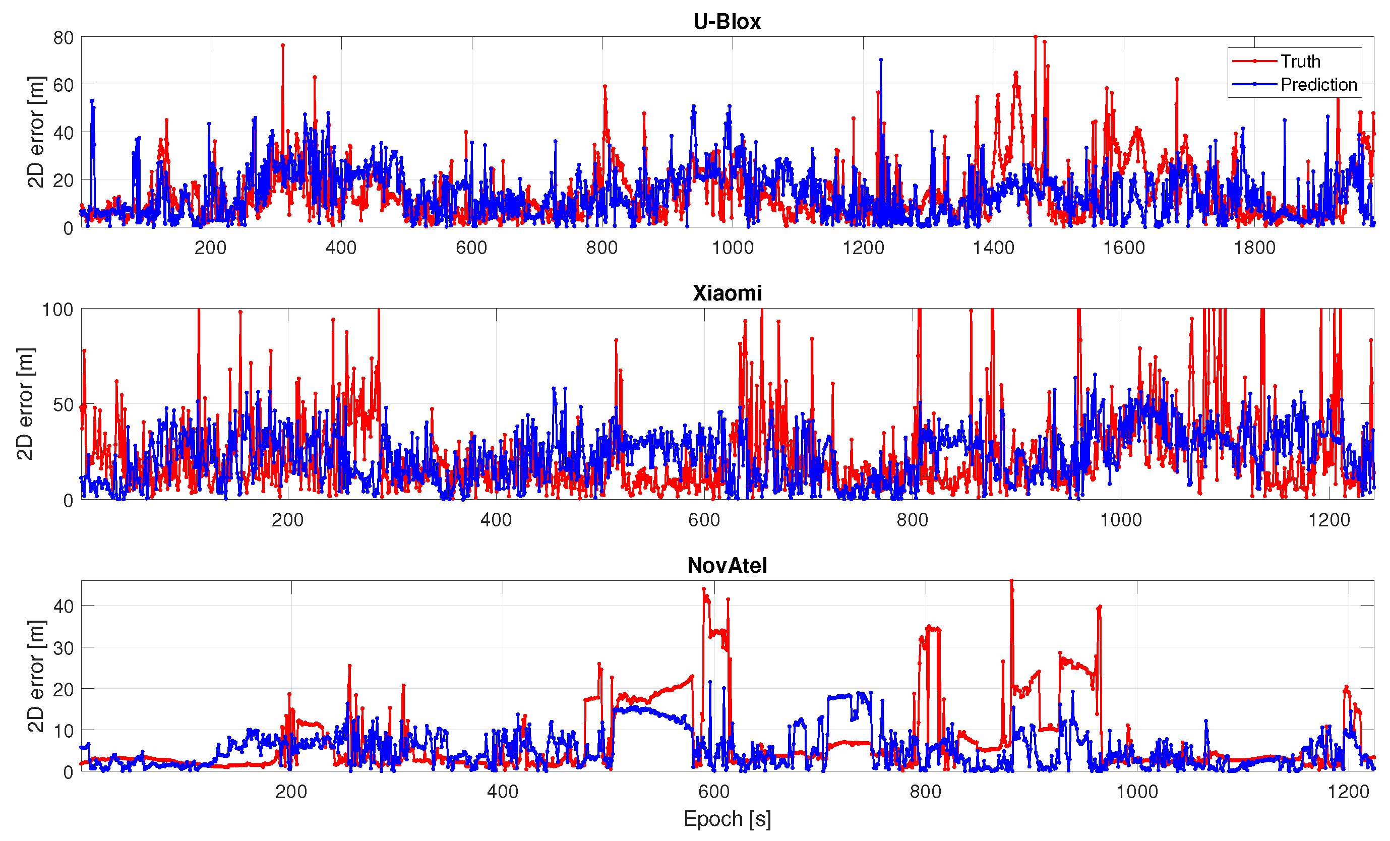
The training processes for all receivers show convergence, with the final loss being less than 0.1. The stochastic gradient descent method (SGDM) was used to search for optimal learnable parameters and biases that minimize the loss function [47]. The initial learning rate of SGDM was set to $1\times {10}^{-5}$, and after every 400 samples, the learning rate will drop by a factor of 0.5 as summarized in the following

Table 3. Training parameters in the CNN model.

Parameters	Details
Minimization algorithm	Stochastic gradient descent momentum
Minimum batch size [samples]	100
Initial learning rate	$1\times {10}^{-4}$
Learning rate drop factor	0.5
Learning rate drop period [samples]	400

. The prediction and truth result of the 2D error for the three GNSS receivers are shown in Figure 6. The prediction accuracy is indicated by the root mean square error (RMSE), defined by:

$$RMSE=\sqrt{\frac{1}{N}{\mathsf{\Sigma }}_i^N{(x_{prediction}^i-x_{truth}^i)}^2},$$

(28)

where N stands for the total number of calculated epochs and i is the epoch index at which $x_{prediction}^i$ and $x_{truth}^i$ denote the predicted and true uncertainty values.

The overall evaluation in RMSE has also been summarized in

Table 4. Training parameters in the CNN model.

Metrics	U-Blox	Xiaomi	NovAtel
RMSE [m]	13.50	52.71	8.78

. The RMSE for Xiaomi data (52.71 m) is the highest, while NovAtel is the lowest (8.78 m) and U-Blox lies in the middle (13.50 m). The main reason may come from the different qualities of the three receivers. Xiaomi has the most and highest noise in the positioning, while NovAtel has the least and U-Blox has the middle level. The CNN model with limited training datasets can hardly generate precise extreme predictions in epochs with occasionally large positioning errors (higher than 100 m). Therefore, the overall RMSE will be elevated for the receiver with more significant noise, especially for the performance of Xiaomi. Nevertheless, the different performance of CNN prediction across the three receivers would differently impact the adaptation quality on solution uncertainty for GNSS/INS integration.

It is noted that a different total number of epochs exists for the data of three receivers due to the different GNSS availability. This is defined by the ratio between the number of available GNSS epochs ($N_{GNSS}$ ) and the number of all calculated epochs ($N_{All}$), as in the expression:

$$GNSSAvailability=\frac{N_{GNSS}}{N_{All}}.$$

(29)

4.2.2. Integration Validation Using U-Blox Data

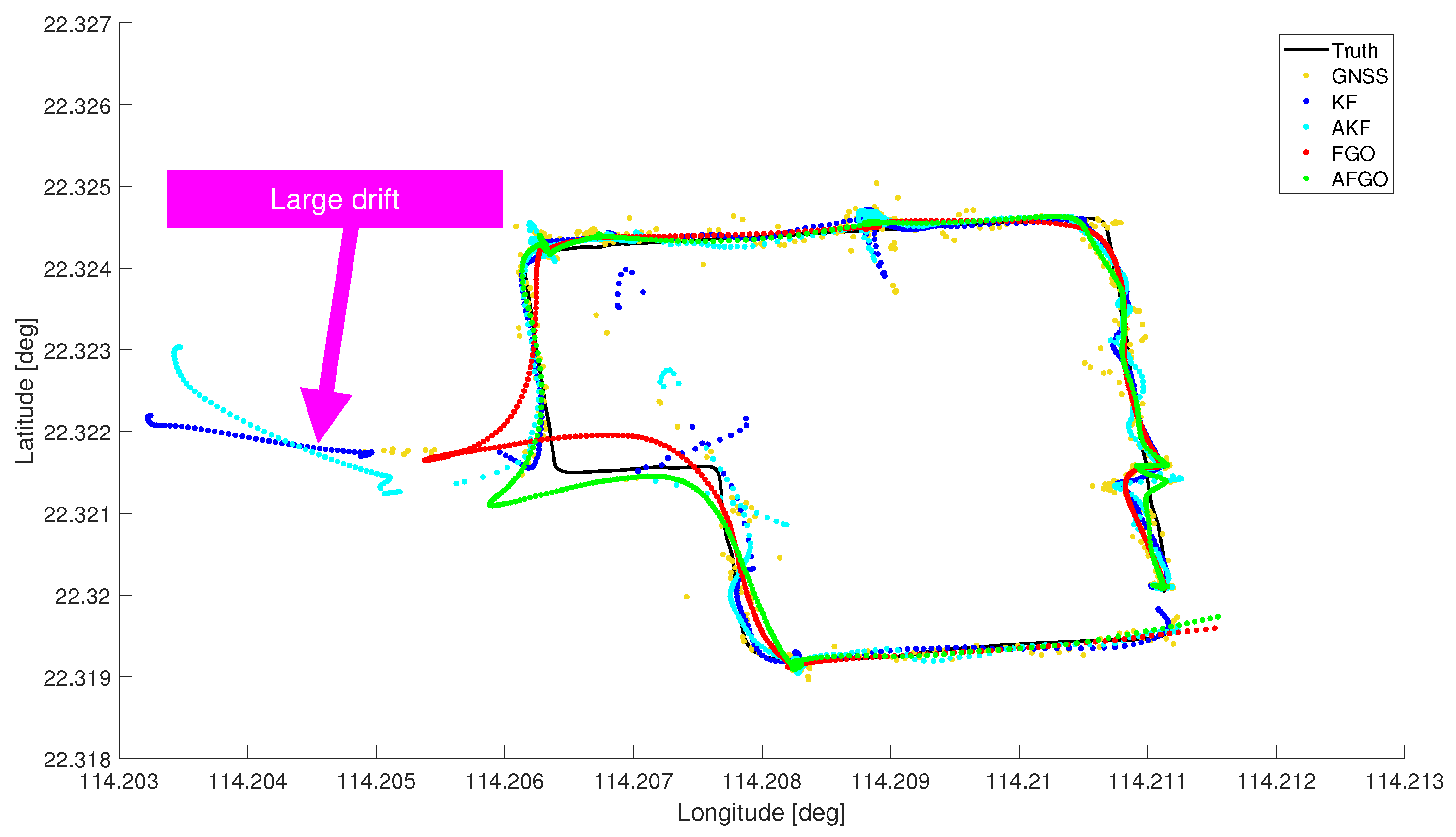
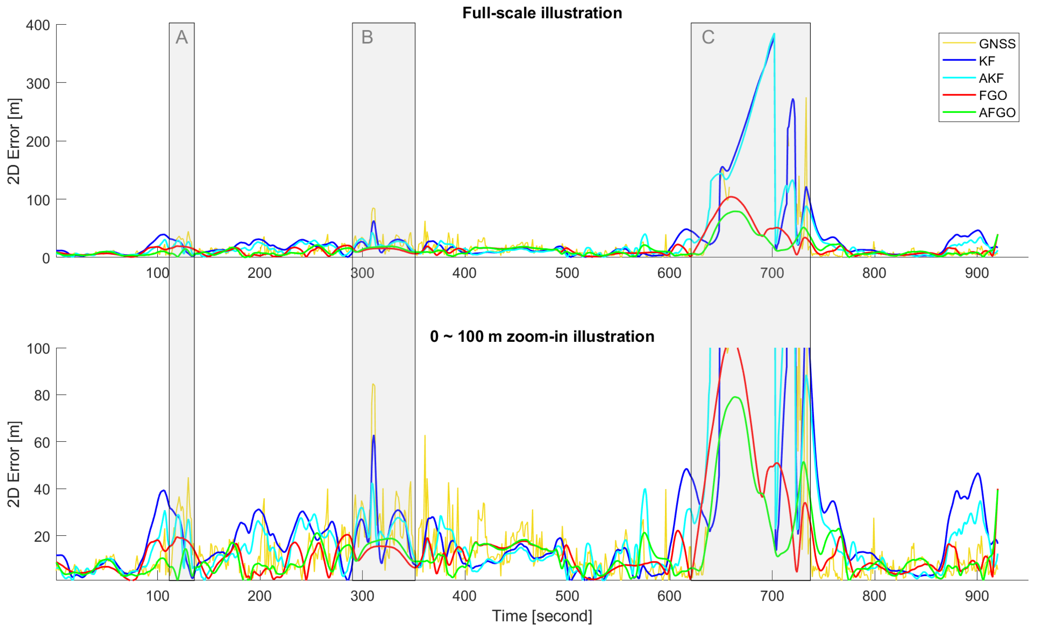
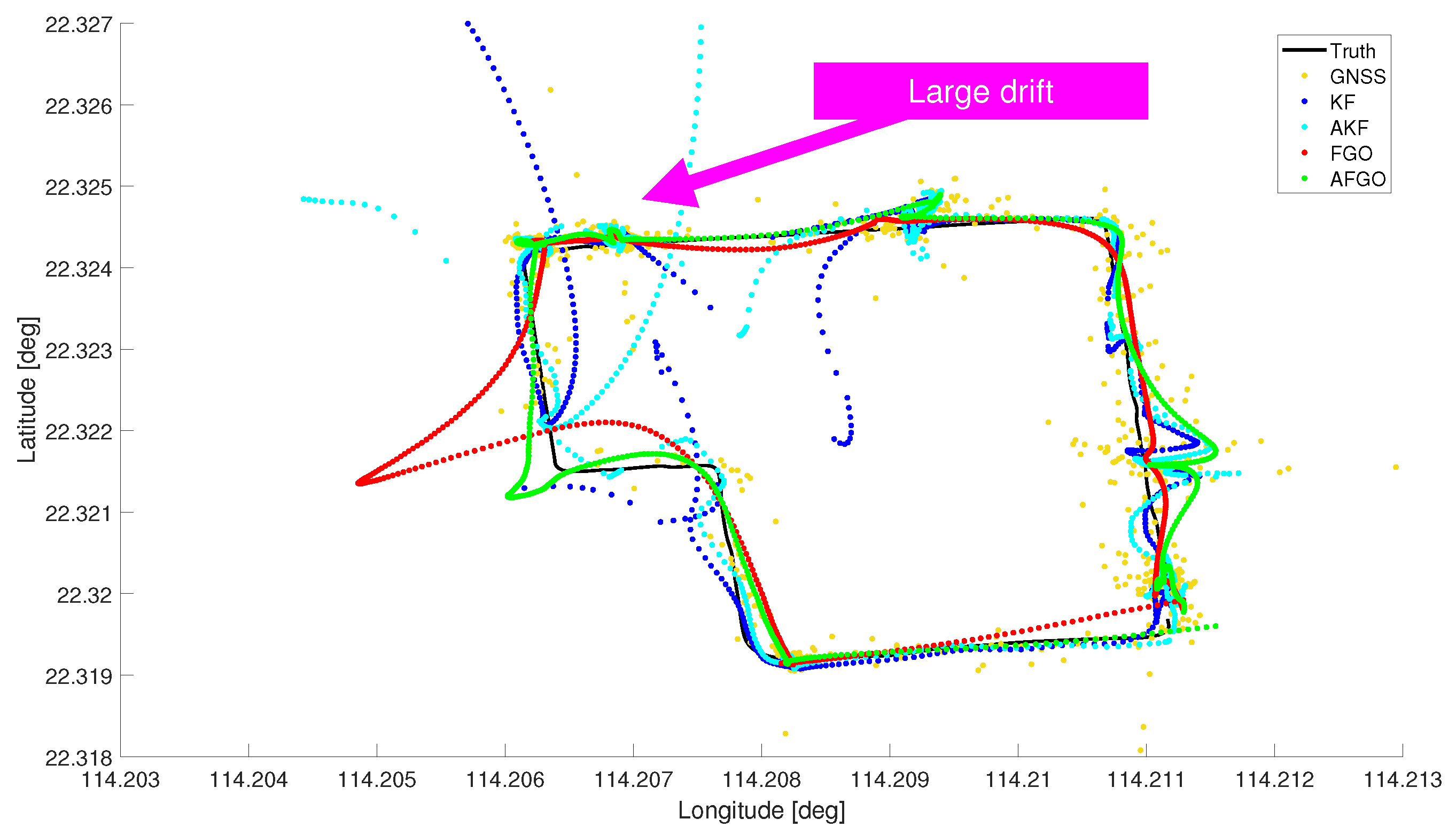
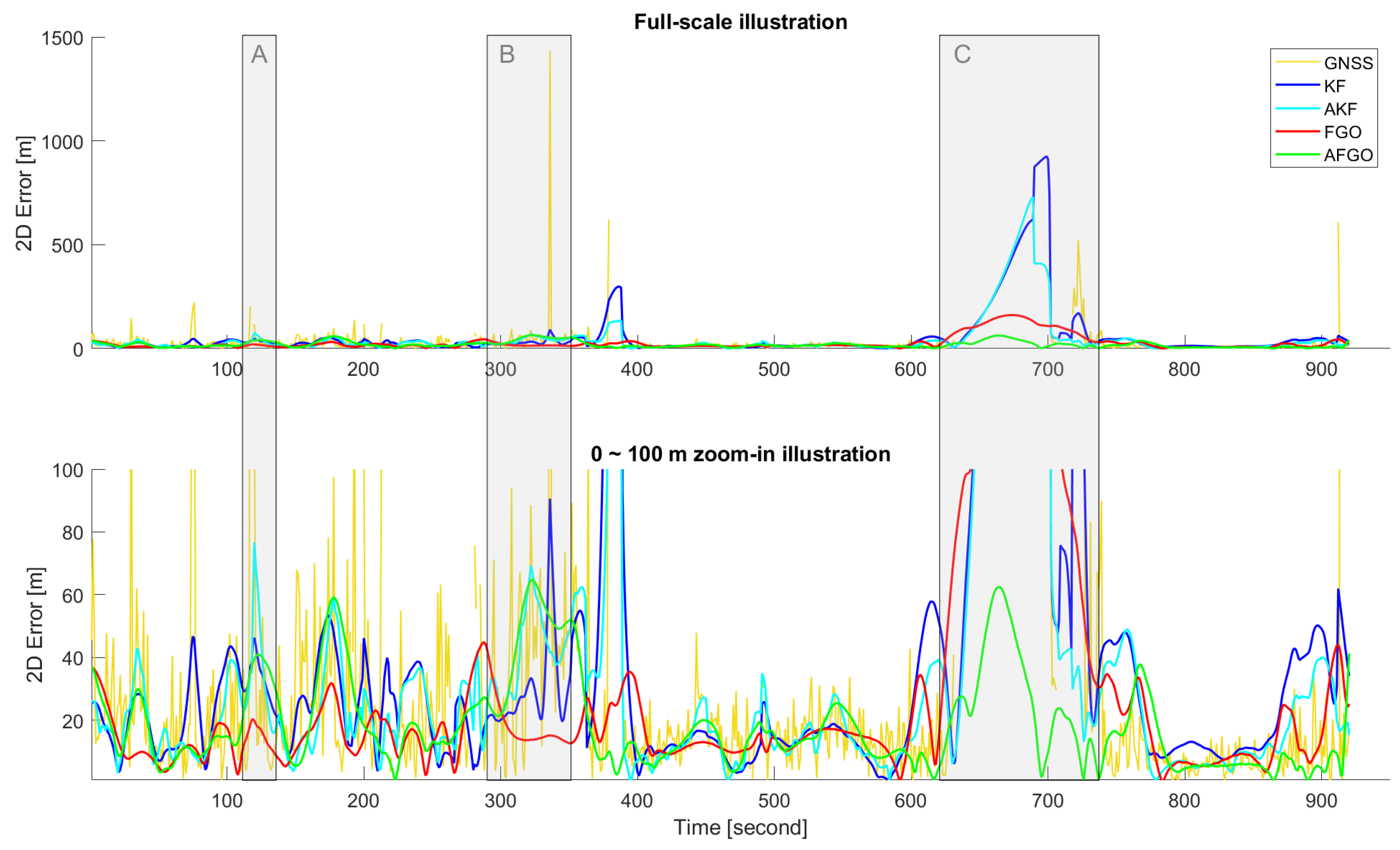
The 2D trajectories of ground truth and different navigation solutions (i.e., GNSS, KF, AKF, FGO, and AFGO) are shown in Figure 7, while Figure 8 provides the 2D positioning error of these solutions along the whole path. Based on the results of the 2D solutions, the RMSE throughout 920 s and the standard deviation (STD) of the 2D errors are proposed for evaluation and are shown in

Table 5. Overall evaluations on GNSS solutions and GNSS/INS integration, including KF, AKF, FGO, and AFGO, for U-Blox data.

Metrics	GNSS	KF	AKF	FGO	AFGO
2D RMSE [m]	26.39	70.18	66.84	24.35	19.35
2D STD [m]	22.30	61.72	59.19	18.71	14.09
Number of epochs with available solutions	852	920	920	920	920
Average computational time [s]	–	$7.93\times {10}^{-3}$	$8.13\times {10}^{-3}$	$7.38\times {10}^{-1}$	$7.52\times {10}^{-1}$

along with the information of the number of available GNSS epochs and integration time. The smaller the values of RMSE and STD, the more accurate the navigational solutions and the smoother trajectory there could be. Some features in U-Blox outcomes will be analyzed as the following. At all three junctions A, B, and C stated in Figure 5, the 2D trajectories in Figure 7 show observable drifts, and Figure 8 shows that the 2D positioning errors in the shaded junction periods increase compared with the surrounding epochs. Especially at junction C (roughly second 630–730), large drift and a 2D positioning error of over 350 m happens for integration methods when missing multiple GNSS epochs. This could be caused by the INS transition without a GNSS update, and error is thus accumulated with time elapsing. However, FGO and AFGO significantly outperform KF-based methods by avoiding the large drifts shown in the shaded area C in Figure 8. This can be connected with the advantage of FGO, which estimates states more precisely by considering all historical epochs.

Additionally, although Figure 8 shows that the performance of the four GNSS/INS integration methods (i.e., KF, AKF, FGO, and AFGO) varies on the time frame, the overall RMSE and STD results in Table 5 proves that accuracy and smoothness improve across the integration methods (from KF to AFGO). Both RMSE and STD using AFGO are reduced to less than 33.3% of those based on KF. It is noted that the RMSE (26.39 m) and STD (22.30 m) of GNSS prove to be smaller than those of KF (70.18 m RMSE and 61.72 m STD) and AKF (66.84 m RMSE and 59.19 m STD). This is acceptable because only 852 epochs with available positioning information are evaluated in the GNSS solution. In contrast, as for integration methods, all 920 epochs are processed with either GNSS/INS coupling or INS propagation, thus inducing a larger calculated RMSE and STD. Moreover, the average computational time for each of the integration methods has been calculated using the equation:

$$Averagecomputationaltime=\frac{t_{total}}{920}$$

(30)

where $t_{total}$ refers to the total computational time for the GNSS/INS integration of 920 epochs. This decreasing update rate from KF to AFGO indicates an increasing total computational time. This coincides with our expectation that the FGO algorithm and adaptive uncertainty settings will take extra time.

Notably, although the trajectory of this study covers multiple urban environments, it has the constraints of short duration (920 s in total) and a limited number of measured epochs (852 epochs). The evaluation for the other two receivers (i.e., Xiaomi and NovAtel) with similar cases will be discussed in the following paragraphs.

4.2.3. Integration Validation Using Xiaomi Data

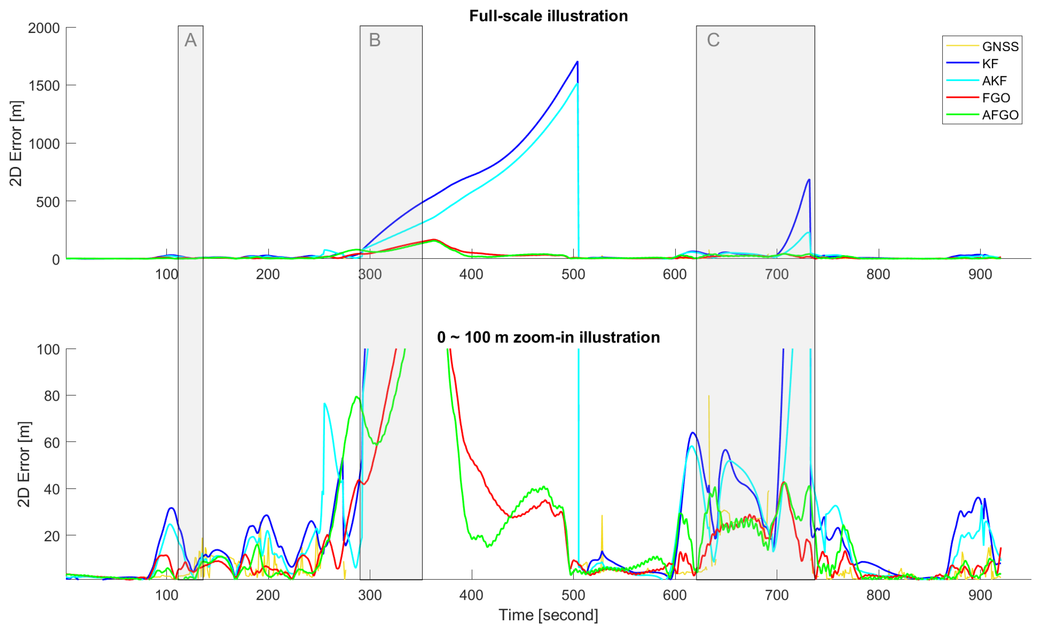
The 2D trajectories shown in Figure 9 overall fluctuate more significantly away from truth than the U-Blox results, and an extremely large (over 1000 m) 2D error from GNSS and KF-based integration methods can be found in some epochs in Figure 10. Compared with the U-Blox receiver, the results of Xiaomi in

Table 6. Overall evaluations on GNSS solutions and GNSS/INS integration, including KF, AKF, FGO, and AFGO, for the Xiaomi data.

Metrics	GNSS	KF	AKF	FGO	AFGO
2D RMSE [m]	84.30	140.61	108.47	42.85	23.89
2D STD [m]	79.32	128.99	98.47	33.49	14.88
Number of epochs with available solutions	795	920	920	920	920
Average computational time [s]	–	$6.92\times {10}^{-3}$	$7.01\times {10}^{-3}$	$5.97\times {10}^{-1}$	$6.33\times {10}^{-1}$

also exhibit larger values in both the RMSE and STD for each of the integration methods. All of those indicate a larger positioning error and less smoothness and coincides with the expectation that Xiaomi has a larger solution uncertainty than U-Blox.

The results also depict that the 2D error at all junctions are larger than those of U-Blox. It is noted that at junction C, significant drift in Figure 9 from the truth trajectory and an extremely large (over 1500 m) 2D positioning error in Figure 10 occurs. Similar to U-Blox, this large drift can be caused by the propagation with INS data only when GNSS becomes unavailable. Other reasons behind it may involve the longest waiting time (i.e., around 100 s) without GNSS information among the three junctions as well as the large uncertainty characteristics of the Xiaomi GNSS receiver and the poor-quality built-in IMU. Nevertheless, due to the robustness given by more historical information, the FGO-based methods still eliminate the large drift (corresponding to the shaded area C in Figure 10) occurring in KF and AKF solutions. AFGO outperforms the original GNSS positioning and still provides the best positioning solutions in terms of both RMSE and STD among the GNSS/INS integration methods. Moreover, the GNSS information of Xiaomi becomes less available compared with the U-Blox receiver, and this may result in shorter computational time for all integration methods, as demonstrated in Table 6.

4.2.4. Integration Validation Using NovAtel Data

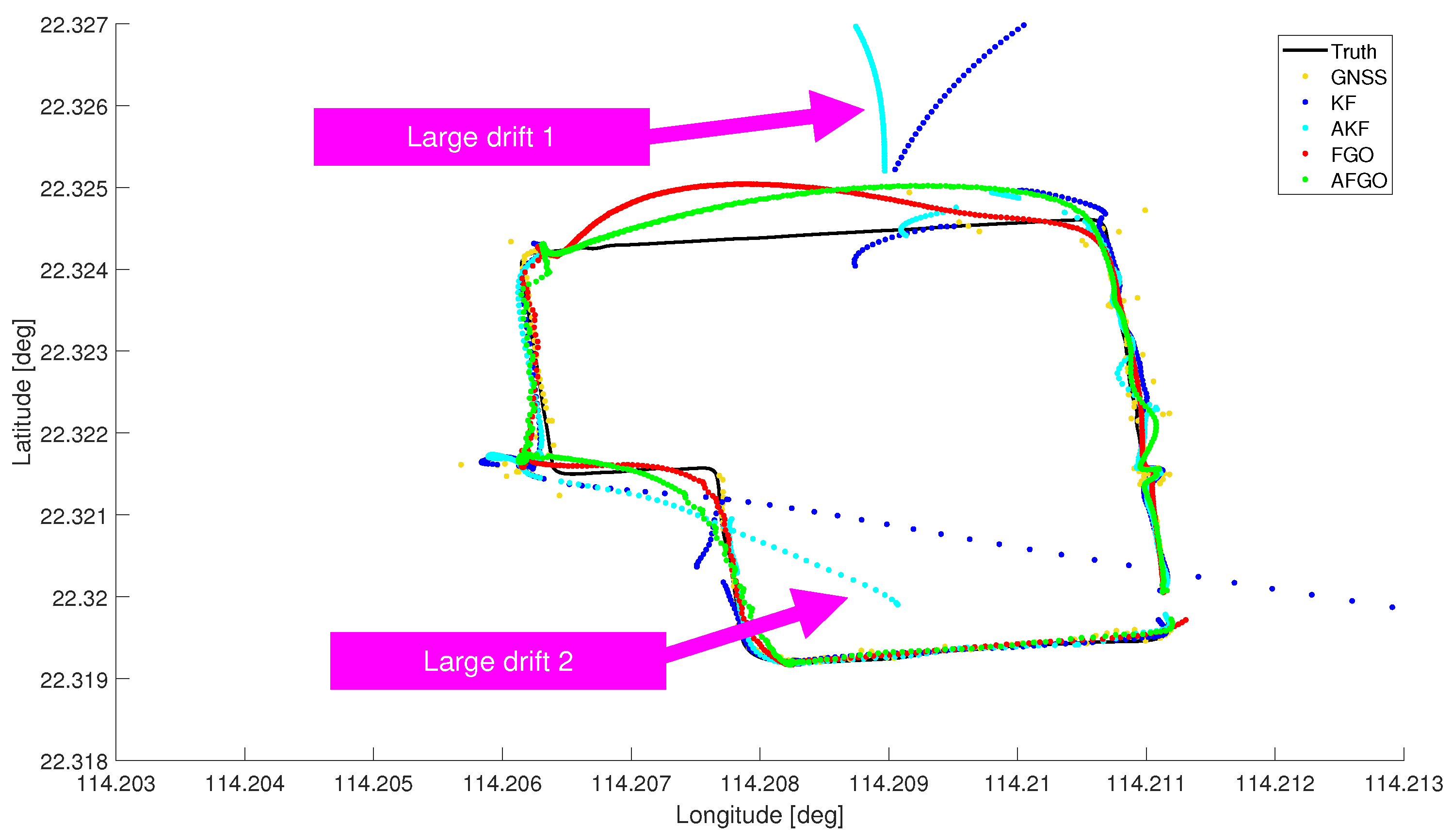
Among the three receivers, NovAtel misses the most GNSS epochs. With only 622 remaining epochs available, integration methods using NovAtel data cost the shortest computational time as well. Among the three discussed receivers, although NovAtel with the lowest GNSS availability of 67.6% (i.e., 622/920) generates the highest RMSE and STD shown in

Table 7. Overall evaluations of GNSS solutions and GNSS/INS integration, including KF, AKF, FGO, and AFGO, for NovAtel data.

Metrics	GNSS	KF	AKF	FGO	AFGO
2D RMSE [m]	10.36	424.52	358.47	40.26	38.20
2D STD [m]	8.24	374.62	320.72	33.61	31.00
Number of epochs with available solutions	622	920	920	920	920
Average computational time [s]	–	$6.54\times {10}^{-3}$	$6.76\times {10}^{-3}$	$5.65\times {10}^{-1}$	$5.76\times {10}^{-1}$

, this receiver provides the closest fit trajectory to the ground truth as depicted in Figure 11 and the lowest 2D error according to Figure 12 when GNSS information becomes available. Likewise, the large positioning drifts of KF-based methods shown in Figure 11 are mitigated by the more robust FGO algorithm, and this significantly improves the accuracy and smoothness. This is reflected in Table 7, where the RMSE and STD levels of FGO and AFGO are approximately 10% of those in AKF and AKF, respectively.

For a more detailed analysis of the two existing drifts, at junction A (roughly second 110–130), neither a significant trajectory drift nor large 2D error occur, but these appear at junctions B (roughly second 290–350) and C (roughly second 630–730) given that many epochs with GNSS positioning are missing. Available GNSS epochs are particularly sparse around junction B, and the positioning performance of the NovAtel receiver is even negatively impacted after passing the crossroad (i.e., shaded area of Junction B in Figure 12). This even results in a larger error accumulated using the INS transition only, thus causing a more extreme positioning drift than those at the subsequent junction C. This comparison is reflected in the two large drifts in Figure 11 and the two peaks around roughly second 500 and 730 of Figure 12.

5. Further Analysis and Evaluation

5.1. Comparisons between Receivers and across Integration Methods (KF-Based vs. FGO-Based)

This section compares the positioning results across the three GNSS receivers in terms of the RMSE of the solutions and STD of the 2D error. With reference to KF, the positioning improvement on the RMSE and STD of the other three integration methods are introduced in:

$$\begin{array}{c}RMS{E}_{improvement\%}=\frac{RMS{E}_{method}-RMS{E}_{KF}}{RMS{E}_{KF}}\times 100\%,\end{array}$$

(31)

$$\begin{array}{c}ST{D}_{improvement\%}=\frac{ST{D}_{method}-ST{D}_{KF}}{ST{D}_{KF}}\times 100\%,\end{array}$$

(32)

where the subscript “method” may denote AKF, FGO, or AFGO. It is noted that the RMSE and STD of the GNSS solution are not taken as the reference because those should have been infinity given the missing GNSS epochs; thus, further improvement based on GNSS is unreasonable to evaluate.

Combined with Figure 13a showing the GNSS availability defined in Equation (21), graphs on the RMSE and STD of different integration methods are given in Figure 13b and Figure 13c, respectively. It is displayed that GNSS availability decreases from U-Blox (92.61%) to Xiaomi (86.41%) to NovAtel (67.61%), whereas the bar charts about RMSE and STD improvement for each receiver basically show the opposite relationship, which rises from U-Blox (red) to Xiaomi (magenta) to NovAtel (blue). Overall, compared with KF, the less the GNSS availability, the greater the improvements in both RMSE and STD tend to happen for each of the methods (i.e., AKF/FGO/AFGO). Despite the anomaly for the AKF method where Xiaomi has greater improvements in the RMSE and STD than NovAtel, the results could reflect that the receiver with less GNSS availability would potentially benefit more from GNSS/INS integration in terms of positioning accuracy and smoothness as greater improvements would be achieved according to Figure 13b,c.

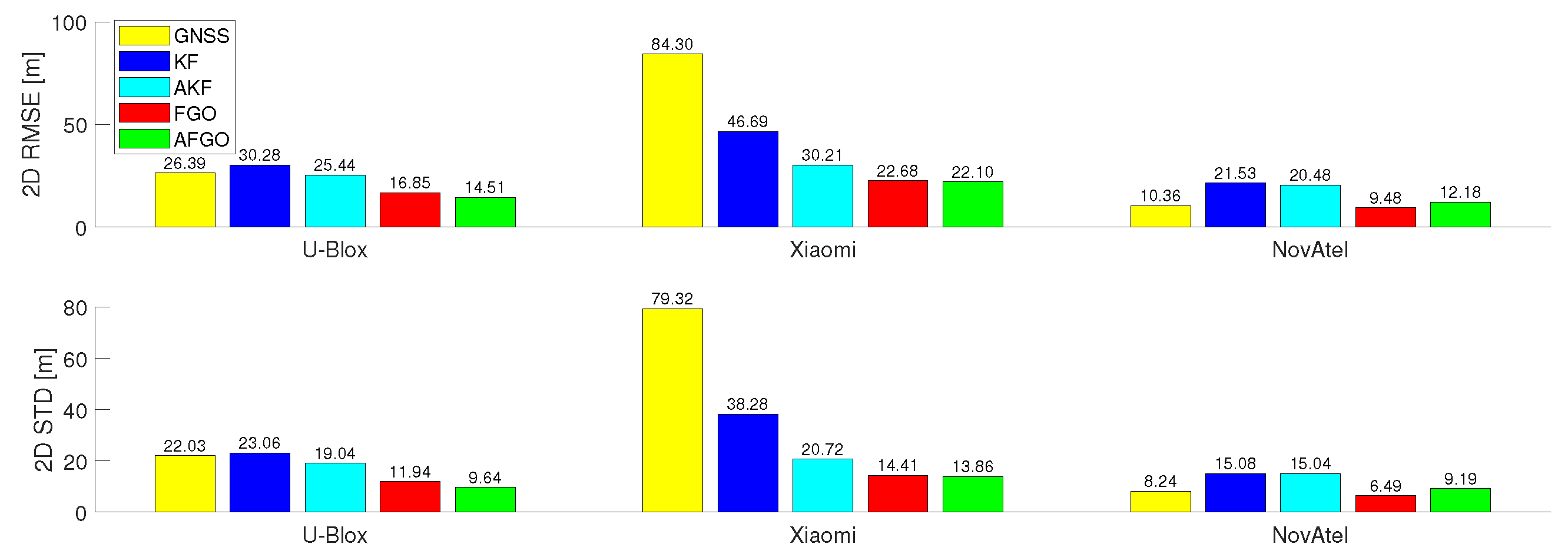
Moreover, in Figure 13, the improvements from AKF (all below 25%) appear less significant than those given by FGO-based methods (all over 65%). Possible explanations may lie in that the GNSS unavailability causes free propagation using INS data. In contrast from KF-based methods, which accumulate the errors during INS transition, FGO-based solutions are less constrained on the missing GNSS epochs and are less likely to produce positioning drifts, thus giving higher improvement in both the RMSE and STD. This is also revealed in the bar chart in Figure 14, which summarizes the 2D RMSE and STD of the four integration methods during all 920 s. The FGO and AFGO methods have less 2D RMSE and less 2D STD for all three receivers, which means a higher accuracy and smoother solutions compared with KF and AKF. Especially for Xiaomi and NovAtel, as shown in Figure 14, FGO-based solutions have a significant decrease (approximately ranging from 70% to 95%) in both the RMSE and STD from KF-based ones, and these are also reflected in the results of Figure 13b,c. Additionally, according to Figure 7, Figure 9 and Figure 11, at junctions where large trajectory drifts exist, the 2D positioning error results in Figure 8 (Junction C), Figure 10 (junction C), and Figure 12 (junction B and C) roughly reveal that the FGO and AFGO curves are far below those of KF and AKF. For Xiaomi and NovAtel, which have more extreme positioning drifts than U-Blox, this situation seems more evident. It should also be mentioned that AFGO (FGO-based) proves to be the most accurate and stable method amongst all integration methods, having the lowest 2D RMSE and STD for all grades of GNSS receivers.

Apart from the discussion on the overall 920 epochs, the evaluation comparing receivers and integration methods is given in Figure 15 only using epochs with available GNSS information. It depicts that all GNSS/INS integration methods still outperform GNSS in terms of the 2D RMSE and STD for Xiaomi. As for U-Blox and NovAtel, integration methods (e.g., KF in U-Blox, and methods except FGO in NovAtel) may perform either less accurately (higher RMSE) or less smoothly (higher STD) than GNSS. Possible explanations are that integration methods applied on the certain receiver still require the GNSS updates for several additional epochs once GNSS becomes available again after outage before coming back to the normal level of positioning errors. Such “recovery periods”, counted as the GNSS-available epochs for the evaluation in Figure 15, would elevate the overall RMSE and STD. Different from the full evaluation using 920 epochs, the only anomaly in Figure 15 stopping us from concluding that AFGO generates the best solutions is that AFGO has a higher RMSE and STD than FGO for the NovAtel receiver. This is anticipated because of NovAtel’s worst GNSS availability while having the most accurate GNSS positionings among the three receivers when free from outage. Balance between these two aspects would demand instant and precise uncertainty adaptations based on CNN predictions. However, such low-tolerance targets would hardly be feasible with our limited-quality CNN model when helping to further improve FGO towards a better performance than the GNSS solutions with low RMSE and STD. Nevertheless, in terms of the overall performance of 920 epochs (in Figure 14), which contains both the GNSS outage and GNSS-available scenarios, AFGO still provides the best performance among integration methods for NovAtel data.

5.2. Analysis between Fixed and Adaptive Integrations

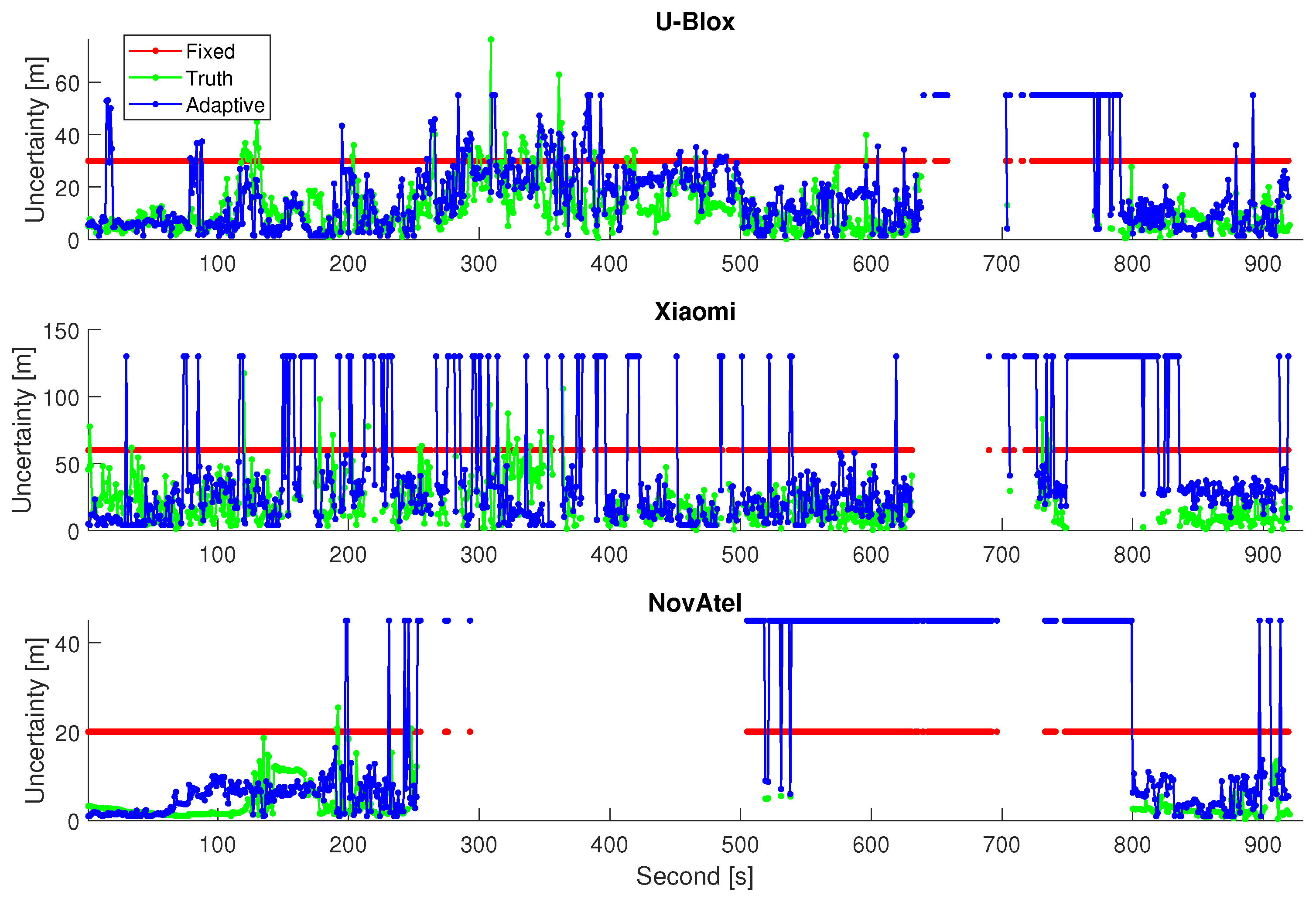
As mentioned above, considering all 920 s, adaptive uncertainty solutions (i.e., AKF and AFGO) have a lower RMSE and STD than the corresponding fixed uncertainty solutions (i.e., KF and FGO), which indicates that adaptive solutions have more accuracy and smoothness. This could be explained, incorporated with Figure 16, that adaptive solutions provide uncertainty (marked in blue) that are tailored by the fast-changing urban environment and are closer to the actual 2D error or truth uncertainty (marked in green). These can potentially handle more scenarios than solutions with a single fixed uncertainty (marked in red) throughout the period.

Figure 17 presents the adaptive, fixed, and truth uncertainty for all discussed receivers. The curves are sometimes discontinuous due to the lack of available GNSS epochs and the uncertainties without CNN prediction due to extreme feature values are set to be the “Max uncertainty”, while “Min uncertainty” is employed as the allowable lowest value of uncertainty. A typical short duration from second 162 to 167 in Figure 17 has been particularly selected as the example to showcase the differences between fixed and adaptive settings on the solution uncertainty. It can be seen in the subfigures of Figure 17a about U-Blox and Figure 17c about NovAtel that adaptive uncertainty is closer and shares a similar decreasing trend with the truth compared with the curve of fixed uncertainty. As for Xiaomi, shown in Figure 17b, the missing CNN prediction from second 164 to 167 indicates the poor data quality. The fixed uncertainty will not change according to the GNSS context, while the adaptive uncertainty surges intelligently to the “Max uncertainty” 130 m, which is assumed to be more approximated to the true uncertainty.

6. Conclusions and Future Research Direction

This paper compares different GNSS/INS integration methods based on KF and FGO to process data from different levels of receivers (i.e., U-Blox, Xiaomi, and NovAtel). Despite being impacted by the quality of the trained deep learning model, the choice of uncertainty parameters (e.g., fixed, min, and max uncertainty), and limited duration (920s) with less evaluated epochs, the proposed MATLAB-implemented AFGO shows the promising capability to adaptively generate the most accurate (in terms of RMSE) and smooth (in terms of STD) solutions for all level of receivers among all discussed integration methods (i.e., KF, AKF, FGO, and AFGO).

The current limitations partly come from a diversity of GNSS receivers because CNN models are trained separately across different receivers and are then employed to adaptively assist GNSS/INS integrations. Future work should include a generalized adaptation model in the AFGO architecture for all grades of receivers and should validate the feasibility and advantages of AFGO in a wider range of urbanization scenarios. Additionally, there can be large residuals between the truth and predicted solution uncertainty, indicating the necessity to propose better-functioning deep learning models. This could be potentially realized through various methods, including introducing more effective features, upgrading the network structure using methods such as optimizing the types and number of layers, and training through a larger amount of urban GNSS data. Moreover, the GNSS measurements like Doppler are related to the user dynamics. Thus, extending the proposed network for GNSS-based motion detection to compensate for INS error is worth investigating in the future. The implementation of the proposed algorithm in practical applications is also worth investigating in the future, where additional algorithms to reduce the computation load, such as the sliding window [11], may need to be developed.

References

1. Zimmermann, F. Analysis and Mitigation of Site-Dependent Effects in Static and Kinematic GNSS Applications. Ph.D. Thesis, Rheinische Friedrich-Wilhelms—Universitat Bonn, Bonn, Germany, 2019. [Google Scholar]
2. Avram, A.; Schwieger, V.; Gemayel, N.E. Experimental results of multipath behavior for GPS L1-L2 and Galileo E1-E5b in static and kinematic scenarios. J. Appl. Geod. 2019, 13, 279–289. [Google Scholar] [CrossRef]
3. Wang, E.; Cai, M.; Pang, T. A Simple and Effective GPS Receiver Autonomous Integrity Monitoring and Fault Isolation Approach. In Proceedings of the 2012 International Conference on Control Engineering and Communication Technology, Shenyang, China, 7–9 December 2012; pp. 657–660. [Google Scholar] [CrossRef]
4. Baasch, K.N.; Icking, L.; Ruwisch, F.; Schön, S. Coordinate Frames and Transformations in GNSS Ray-Tracing for Autonomous Driving in Urban Areas. Remote Sens. 2023, 15, 180. [Google Scholar] [CrossRef]
5. Lau, L.; Cross, P. Development and testing of a new ray-tracing approach to GNSS carrier-phase multipath modelling. J. Geod. 2007, 81, 713–732. [Google Scholar] [CrossRef]
6. Lee, M.J.L.; Lee, S.; Ng, H.F.; Hsu, L.T. Skymask Matching Aided Positioning Using Sky-Pointing Fisheye Camera and 3D City Models in Urban Canyons. Sensors 2020, 20, 4728. [Google Scholar] [CrossRef] [PubMed]
7. Aboutaleb, A.; El-Wakeel, A.S.; Elghamrawy, H.; Noureldin, A. LiDAR/RISS/GNSS Dynamic Integration for Land Vehicle Robust Positioning in Challenging GNSS Environments. Remote Sens. 2020, 12, 2323. [Google Scholar] [CrossRef]
8. Chiang, K.W.; Tsai, G.J.; Li, Y.H.; Li, Y.; El-Sheimy, N. Navigation Engine Design for Automated Driving Using INS/GNSS/3D LiDAR-SLAM and Integrity Assessment. Remote Sens. 2020, 12, 1564. [Google Scholar] [CrossRef]
9. Wan, G.; Yang, X.; Cai, R.; Li, H.; Zhou, Y.; Wang, H.; Song, S. Robust and Precise Vehicle Localization Based on Multi-Sensor Fusion in Diverse City Scenes. In Proceedings of the IEEE International Conference on Robotics and Automation (ICRA), Brisbane, QLD, Australia, 21–25 May 2018; pp. 4670–4677. [Google Scholar] [CrossRef]
10. Cao, S.; Lu, X.; Shen, S. GVINS: Tightly Coupled GNSS–Visual–Inertial Fusion for Smooth and Consistent State Estimation. IEEE Trans. Robot. 2022, 38, 2004–2021. [Google Scholar] [CrossRef]
11. Wen, W.; Pfeifer, T.; Bai, X.; Hsu, L.T. Factor graph optimization for GNSS/INS integration: A comparison with the extended Kalman filter. NAVIGATION J. Inst. Navig. 2021, 68, 315–331. [Google Scholar] [CrossRef]
12. Falco, G.; Pini, M.; Marucco, G. Loose and Tight GNSS/INS Integrations: Comparison of Performance Assessed in Real Urban Scenarios. Sensors 2017, 17, 255. [Google Scholar] [CrossRef]
13. Gao, G.; Lachapelle, G. A novel architecture for ultra-tight HSGPS-INS integration. J. Glob. Position. Syst. 2008, 7, 46–61. [Google Scholar] [CrossRef]
14. Wang, G.; Han, Y.; Chen, J.; Wang, S.; Zhang, Z.; Du, N.; Zheng, Y. A GNSS/INS Integrated Navigation Algorithm Based on Kalman Filter. IFAC-PapersOnLine 2018, 51, 232–237. [Google Scholar] [CrossRef]
15. Wu, Y.; Chen, S.; Yin, T. GNSS/INS Tightly Coupled Navigation with Robust Adaptive Extended Kalman Filter. Int. J. Automot. Technol. 2022, 23, 1639–1649. [Google Scholar] [CrossRef]
16. Zhang, G.; Hsu, L.T. Intelligent GNSS/INS integrated navigation system for a commercial UAV flight control system. Aerosp. Sci. Technol. 2018, 80, 368–380. [Google Scholar] [CrossRef]
17. Kim, J.W.; Hwang, D.H.; Lee, S.J. A Deeply Coupled GPS/INS Integrated Kalman Filter Design Using a Linearized Correlator Output. In Proceedings of the 2006 IEEE/ION Position, Location, and Navigation Symposium, San Diego, CA, USA, 25–27 April 2006; pp. 300–305. [Google Scholar] [CrossRef]
18. Wan, E.; Van Der Merwe, R. The unscented Kalman filter for nonlinear estimation. In Proceedings of the IEEE 2000 Adaptive Systems for Signal Processing, Communications, and Control Symposium (Cat. No.00EX373), Lake Louise, AB, Canada, 4 October 2000; pp. 153–158. [Google Scholar] [CrossRef]
19. Hu, G.; Gao, S.; Zhong, Y. A derivative UKF for tightly coupled INS/GPS integrated navigation. ISA Trans. 2015, 56, 135–144. [Google Scholar] [CrossRef] [PubMed]
20. Wang, J.; Chen, X.; Shi, C. A novel robust iterated CKF for GNSS/SINS integrated navigation applications. EURASIP J. Adv. Signal Process. 2023, 2023, 83. [Google Scholar] [CrossRef]
21. Liu, J.; Cai, B.g.; Tang, T.; Wang, J. A CKF based GNSS/INS train integrated positioning method. In Proceedings of the 2010 IEEE International Conference on Mechatronics and Automation, Xi’an, China, 4–7 August 2010; pp. 1686–1689. [Google Scholar] [CrossRef]
22. Jwo, D.J.; Chung, F.C.; Yu, K.L. Interacting Multiple Model Particle Filters for GPS/INS Integration. Appl. Mech. Mater. 2013, 284–287, 2255–2260. [Google Scholar] [CrossRef]
23. Seo, W.; Hwang, S.; Park, J.; Lee, J.M. Precise outdoor localization with a GPS–INS integration system. Robotica 2013, 31, 371–379. [Google Scholar] [CrossRef]
24. Groves, P.D. Principles of GNSS, inertial, and multisensor integrated navigation systems. IEEE Aerosp. Electron. Syst. Mag. 2015, 30, 26–27. [Google Scholar] [CrossRef]
25. Doucet, A.; Johansen, A.M. Particle Filtering and Smoothing: Fifteen Years Later; Oxford University Press: Oxford, UK, 2008. [Google Scholar]
26. Dellaert, F. Factor Graphs and GTSAM: A Hands-on Introduction; Georgia Institute of Technology: Atlanta, GA, USA, 2012. [Google Scholar]
27. Li, M.; Hu, K.; Liu, Y.; Hu, E.; Tang, C.; Zhu, H.; Zhou, G. A Multimodal Robust Simultaneous Localization and Mapping Approach Driven by Geodesic Coordinates for Coal Mine Mobile Robots. Remote Sens. 2023, 15, 5093. [Google Scholar] [CrossRef]
28. Xin, S.; Wang, X.; Zhang, J.; Zhou, K.; Chen, Y. A Comparative Study of Factor Graph Optimization-Based and Extended Kalman Filter-Based PPP-B2b/INS Integrated Navigation. Remote Sens. 2023, 15, 5144. [Google Scholar] [CrossRef]
29. Chang, L.; Niu, X.; Liu, T.; Tang, J.; Qian, C. GNSS/INS/LiDAR-SLAM integrated navigation system based on graph optimization. Remote Sens. 2019, 11, 1009. [Google Scholar] [CrossRef]
30. Li, Q.; Zhang, L.; Wang, X. Loosely Coupled GNSS/INS Integration Based on Factor Graph and Aided by ARIMA Model. IEEE Sensors J. 2021, 21, 24379–24387. [Google Scholar] [CrossRef]
31. Zeng, Q.; Chen, W.; Liu, J.; Wang, H. An Improved Multi-Sensor Fusion Navigation Algorithm Based on the Factor Graph. Sensors 2017, 17, 641. [Google Scholar] [CrossRef] [PubMed]
32. Kaess, M.; Johannsson, H.; Roberts, R.; Ila, V.; Leonard, J.; Dellaert, F. iSAM2: Incremental Smoothing and Mapping Using the Bayes Tree. Int. J. Robot. Res. IJRR 2012, 31, 216–235. [Google Scholar] [CrossRef]
33. Yin, Z.; Yang, J.; Ma, Y.; Wang, S.; Chai, D.; Cui, H. A Robust Adaptive Extended Kalman Filter Based on an Improved Measurement Noise Covariance Matrix for the Monitoring and Isolation of Abnormal Disturbances in GNSS/INS Vehicle Navigation. Remote Sens. 2023, 15, 4125. [Google Scholar] [CrossRef]
34. Tao, Y.; Liu, C.; Chen, T.; Zhao, X.; Liu, C.; Hu, H.; Zhou, T.; Xin, H. Real-time multipath mitigation in multi-GNSS short baseline positioning via CNN-LSTM method. Math. Probl. Eng. 2021, 2021, 1–12. [Google Scholar] [CrossRef]
35. Xu, P.; Zhang, G.; Yang, B.; Hsu, L.T. PositionNet: CNN-based GNSS positioning in urban areas with residual maps. Appl. Soft Comput. 2023, 148, 110882. [Google Scholar] [CrossRef]
36. Zawislak, R.; Greiff, M.; Kim, K.J.; Berntorp, K.; Di Cairano, S.; Konishi, M.; Parsons, K.; Orlik, P.V.; Sato, Y. GNSS Multipath Detection Aided by Unsupervised Domain Adaptation. In Proceedings of the 35th International Technical Meeting of the Satellite Division of The Institute of Navigation (ION GNSS+ 2022), Denver, CO, USA, 19–23 September 2022; pp. 2127–2137. [Google Scholar]
37. Dumoulin, V.; Visin, F. A guide to convolution arithmetic for deep learning. arXiv 2018, arXiv:1603.07285. [Google Scholar]
38. Aggarwal, C.C. Neural Networks and Deep Learning: A Textbook; Springer International Publishing: Cham, Switzerland, 2018. [Google Scholar] [CrossRef]
39. Geng, J.; Jiang, E.; Li, G.; Xin, S.; Wei, N. An Improved Hatch Filter Algorithm towards Sub-Meter Positioning Using only Android Raw GNSS Measurements without External Augmentation Corrections. Remote Sens. 2019, 11, 1679. [Google Scholar] [CrossRef]
40. Hsu, L.T.; Kubo, N.; Wen, W.; Chen, W.; Liu, Z.; Suzuki, T.; Meguro, J. UrbanNav: An Open-Sourced Multisensory Dataset for Benchmarking Positioning Algorithms Designed for Urban Areas. In Proceedings of the 4th International Technical Meeting of the Satellite Division of The Institute of Navigation (ION GNSS+ 2021), St. Louis, MO, USA, 20–24 September 2021; pp. 226–256. [Google Scholar] [CrossRef]
41. Rauch, H.E.; Tung, F.; Striebel, C.T. Maximum likelihood estimates of linear dynamic systems. AIAA J. 1965, 3, 1445–1450. [Google Scholar] [CrossRef]
42. Kaplan, E.D.; Hegarty, C. Understanding GPS/GNSS: Principles and Applications, 3rd ed.; Artech House: London, UK, 2017. [Google Scholar]
43. Walter, T.; Enge, P. Weighted RAIM for precision approach. In Proceedings of the 8th International Technical Meeting of the Satellite Division of The Institute of Navigation (ION GPS 1995), Palm Springs, CA, USA, 12–15 September 1995; Institute of Navigation: Manassas, VA, USA, 1995; Volume 8, pp. 1995–2004. [Google Scholar]
44. Ioffe, S.; Szegedy, C. Batch Normalization: Accelerating Deep Network Training by Reducing Internal Covariate Shift. In Proceedings of the 32nd International Conference on Machine Learning, PMLR, Lille, France, 6–11 July 2015; pp. 448–456. [Google Scholar]
45. El-Sheimy, N.; Hou, H.; Niu, X. Analysis and Modeling of Inertial Sensors Using Allan Variance. IEEE Trans. Instrum. Meas. 2008, 57, 140–149. [Google Scholar] [CrossRef]
46. Zhang, G.; Wen, W.; Xu, B.; Hsu, L.T. Extending shadow matching to tightly-coupled GNSS/INS integration system. IEEE Trans. Veh. Technol. 2020, 69, 4979–4991. [Google Scholar] [CrossRef]
47. Cui, N. Applying Gradient Descent in Convolutional Neural Networks. J. Phys. Conf. Ser. 2018, 1004, 012027. [Google Scholar] [CrossRef]
Figure 1. Flowchart of the proposed AFGO approach.
Remotesensing 16 00181 g001
Figure 2. The schematics of a GNSS/INS factor graph. Circles and rectangles represent the states and factors, respectively. The example section at epoch t is displayed to illustrate formulations from (17) to (22).
Remotesensing 16 00181 g002
Figure 3. Overview of the proposed CNN network, where P C N N denotes output from the CNN model.
Remotesensing 16 00181 g003
Figure 4. Illustration of the adaptive uncertainty mechanism.
Remotesensing 16 00181 g004
Figure 5. The anticlockwise ground truth trajectory (green) in Kowloon Bay, Hong Kong. It is separated by breakpoints 1–5 (marked in red) and junctions A, B, and C (marked in yellow). The light, medium, and harsh urban areas are shaded in blue, orange, and purple backgrounds, respectively.
Remotesensing 16 00181 g005
Figure 6. CNN predicted and true 2D positioning error for the three GNSS receivers. The subplot for the Xiaomi receiver has been zoomed in for better illustration. The highest 2D error for the Xiaomi receiver is around 170 m.
Remotesensing 16 00181 g006
Figure 7. Trajectories of different positioning solutions using U-Blox data, with the large drift at junction C being pointed out by the magenta arrow.
Remotesensing 16 00181 g007
Figure 8. 2D positioning errors of different positioning solutions using U-Blox data throughout 920 epochs with the periods at junctions A, B, and C being shaded in gray. The upper subplot depicts the full range of 2D errors, while the lower one shows the zoom-in view from 0 to 100 m.
Remotesensing 16 00181 g008
Figure 9. Trajectories of different positioning solutions using Xiaomi data, with the large drift at junction C being pointed out by the magenta arrow.
Remotesensing 16 00181 g009
Figure 10. 2D positioning errors of different positioning solutions using Xiaomi data throughout 920 epochs, with the periods at junctions A, B, and C shaded in gray. The upper subplot depicts the full range of 2D errors, while the lower one shows the zoom-in view from 0 to 100 m.
Remotesensing 16 00181 g010
Figure 11. Trajectories of different positioning solutions using NovAtel data, with the large drift at junctions B and C being pointed out by the magenta arrow.
Remotesensing 16 00181 g011
Figure 12. 2D positioning errors of different positioning solutions using NovAtel data throughout 920 epochs, with the periods at junctions A, B, and C shaded in gray. The upper subplot depicts the full range of 2D errors, while the lower one shows the zoom-in view from 0 to 100 m.
Remotesensing 16 00181 g012
Figure 13. (a) GNSS availability of the three receivers; improvement of solution performance compared with KF in terms of (b) 2D RMSE and (c) 2D STD. The only anomaly is that for the AKF method, Xiaomi has greater improvements than NovAtel. This is expected because greater improvement comes with lower GNSS availability, which is based on empirical observation rather than strict rules.
Remotesensing 16 00181 g013
Figure 14. Summary of integration methods in terms of the 2D RMSE and STD for the three receivers during all 920 epochs. The data regarding the RMSE and STD come from Table 5, Table 6 and Table 7.
Remotesensing 16 00181 g014
Figure 15. Summary of integration methods in terms of the 2D RMSE and STD for the three receivers during all 920 epochs.
Remotesensing 16 00181 g015
Figure 16. GNSS solution uncertainties of fixed integration (red) and adaptive integration (blue) and the true 2D positioning error indicating the truth uncertainty (green) throughout the time frame for the three receivers. For each receiver, the uncertainties during the GNSS-unavailable period are omitted on all three curves, and only INS propagation is processed. Moreover, the epochs without CNN predictions are particularly omitted on the truth uncertainty curve.
Remotesensing 16 00181 g016
Figure 17. Zoom-in subfigures from Figure 16 during the period 162–167 (second) for the receiver of (a) U-Blox, (b) Xiaomi, and (c) NovAtel.
Remotesensing 16 00181 g017