Abstract
The results of a field experiment devoted to observing slick-band shape variations occurring due to the action of heterogeneous currents related to the passage of internal waves are presented and analyzed on the basis of numerical simulation. The spatiotemporal structure of a train of five solitons of internal waves has been retrieved. Their evolution in the coastal area is demonstrated based on the analysis of propagation characteristics. It is shown that the first soliton, characterized by the higher values of amplitude and width, collapsed when entering shallow water near the observation platform. The parameters of an artificial slick band affected by the passage of internal waves are determined. It is shown that the direction and width of the slick band are related to the direction and magnitude of the upper-ocean horizontal current, which contains a component related to the internal wave. The results of numerical simulation are qualitatively and quantitatively consistent with experimental data at short distances from the platform. An analysis of the conditions responsible for different regimes of slick-band response to the upper-ocean currents generated by propagating internal waves has been performed.
1. Introduction
Heterogeneous upper-ocean currents significantly affect the local and global processes of heat and mass transfer, the distribution of suspended matter and pollution, environmental processes, forecast results and climate models, and require in-depth study [1]. Satellite-based optical and radar sensors receive vast amounts of data on the parameters of the ocean state, but it should be noted that most observations are related to the state of the upper ocean since optical and radar waves are significantly scattered and reflected at the surface inside a thin upper layer. Radar observations of the sea surface demonstrate the presence of irregularities of different scales, related to heterogeneous winds, seabed topography [2], sea currents [3,4] and surfactant pollution [5], which lead to variations in sea surface roughness. Optical images also show irregularities that can additionally be caused by algal blooms, redistribution of suspended matter, and other processes that affect water color (see, for example, [6]). The prospects for solving the inverse problem, namely, retrieval of the characteristics of sea currents from remote sensing data, are described in [7,8,9]. One promising approach is associated with coherent imaging of the sea surface [10]; however, the spatial resolution of the resulting data may be insufficient to observe smaller-scale current irregularities, such as those related to internal waves (IWs).
Variations of the characteristics of the sea surface under the action of propagating IWs can be observed as alternating areas of enhanced and depressed roughness (suloy and slick, respectively). These areas appear due to the action of sub-surface horizontal components of the orbital motion of IWs on small-scale (gravitational-capillary waves) wind waves (see [11,12,13] and references therein). If natural or artificial surfactants are present on the sea surface, then the shape of contaminated areas can be significantly affected by propagating IWs [14]. The disturbance of slick bands, presumably related to natural oil seeps or ship pollution caused by internal waves, is shown in Figure 1.
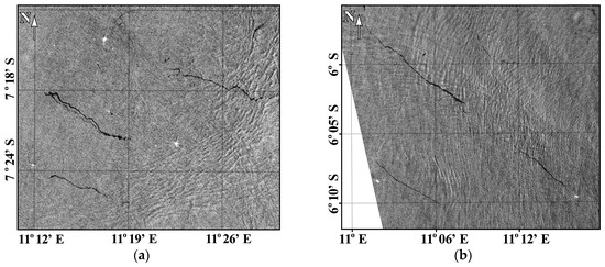
Figure 1.
Extended slick bands in the areas of frequently appearing internal waves: Sentinel-1A, 27 September 2019, 04:52:36 UTC (a); Sentinel-1B, 8 January 2018, 17:33:15 UTC (b).
It can be assumed that the shape of a banded slick structure may allow one to retrieve information about heterogeneous currents related to the IW, which caused a change in its original shape. In addition to the usual retrieval of the kinematic characteristics of IWs [15], this promising and applicable approach may provide additional information about the speed of IW-related homogeneous currents in the upper ocean and the amplitude of IWs.
Previously, in [16,17], an original method for forming an artificial slick band was proposed and developed. It was based on remote detection of the slick-band shape using remote sensing techniques and simultaneous measurements of the upper-ocean sea currents at any point of the slick band. Further experiments in 2019–2021 related to the use of this method were devoted to the observation of various processes in the upper ocean, manifested in the shape of a slick band, as well as the limitations of the proposed method. During one of the experiments, the passage of a train of intense IWs was detected in the Acoustic Doppler Current Profiler (ADCP) signal.
This paper is devoted to the analysis of the experimental data obtained and the results of numerical simulation of IW-related current manifestation in the structure of a slick band in different conditions, as well as a discussion of the dynamics of the slick band.
2. Materials and Methods
2.1. Field Experiments
Field experiments were carried out in the coastal area of the Black Sea from a stationary oceanographic platform in May 2019. The appearance of internal waves is regularly observed and detected near the platform in shallow thermocline conditions. The scheme of experiments with an artificial slick band on 23 May 2019 is shown in Figure 2. Wind conditions can be characterized as moderate, the average wind speed (uw) was about 5 m/s, and the average current speed (uc) was about 7 cm/s. The directions of current (θc) and wind (θw), as well as the direction of IW propagation, are shown schematically in Figure 2.
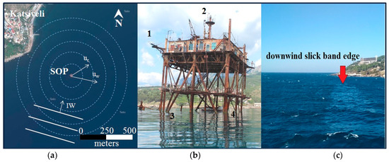
Figure 2.
Scheme of the experiment on 23 May 2019 (a), view of the platform (b) and photograph of the initial stage of the slick band formation (c). 1—X-band coherent radar station, 2—ultrasonic anemometer and weather station, 3—ADCP and 4—surfactant source. The circles correspond to distances from the radar station (grazing angles): 100 m (80.8°), 200 m (85.4°), 300 m (87°), 400 m (87.7°), and 500 m (88.2°). uc, uw, and IW denote the direction of the sea current, wind, and IW front.
The surface manifestation of IWs, related to the redistribution of natural surfactants, and the shape of the artificial slick band were recorded by a digital coherent radar station, MRS-1000 (Micran™, Tomsk, Russia). Accompaning measurements of sea currents were performed with an ADCP WH Monitor 1200 kHz (RDI™, Poway, CA, USA) wind speed was measured using a WindSonic 2D ultrasonic anemometer (Gill Instruments™, Lymington, UK), and other meteorological parameters were recorded using a Vantage Pro2 (Davis Instruments™, Hayward, CA, USA) weather station.
The technique for forming an artificial slick band is based on the continuous deposition of surfactants released from a tank with a single perforation 1.5 mm in diameter, with an almost constant outflow (8–10 mL per min) [16]. To form a slick band, vegetable oil with pre-measured viscoelastic properties of the film (surface tension about 40 mN/m and elasticity 12 mN/m) was used. The released drop of surfactant is shifted by the upper-ocean current and spreads in the tangential direction. A set of falling and spreading drops formed a continuous slick band (photograph in Figure 2). Features of the dynamics of an artificial slick band were described in [16].
2.2. Numerical Simulation
Special software was developed for numerical simulation. A simple kinematic model was programmed using Matlab R2020a. To simulate the propagation of surfactants forming a slick band, we assumed that the upper-ocean current consists of two components, namely, a constant “background” current affected, among other things, by a wind-wave drift (according to [16]) and a propagating disturbance of the current field induced by the IW soliton. More details and numerical simulation results are presented in the corresponding results section.
3. Results
3.1. Characteristics of Internal Waves
ADCP and coherent radar data were used to obtain information about the spatiotemporal structure of IWs. The main attributes of the IW manifestation in the ADCP signal are related to the modulation of vertical profiles of acoustic backscattering and the appearance of significant and coherent vertical and horizontal velocity components. Figure 3 shows a series of acoustic backscatter profiles for each of the four ADCP beams. Beams 1 and 3, directed to the south and west, respectively, did not manifest obstacles related to reflection from platform elements, unlike beams 2 (northward) and 4 (eastward), which were in some cases subject to noise.
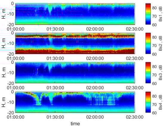
Figure 3.
Acoustic backscattering for each of the four beams of ADCP during the experiment of 23 May 2019, 01:00–02:30 (UTC + 3). Beam 1—southward, beam 2—northward (under the platform), beam 3—westward, and beam 4—eastward.
Unfortunately, measurements of the vertical distribution of temperature and salinity were not available during the described experiment. However, it can be assumed that the position of the layers corresponding to the greatest scattering of sound ensures the position of the pycnocline. According to our long-term observations, in an undisturbed state, this region in May is characterized by a shallow pycnocline at a depth of 3 m. At a depth of more than 16 m, strong stratification with enhanced backscattering is observed.
Figure 3 shows a leading train of three solitons of the highest intensity (t1 = 01:16, t2 = 01:26, and t3 = 01:36) and two retarding solitons of low amplitude (t4 = 01:56 and t5 = 02:14). Since the total depth H near the platform is about 25–30 m, under such conditions the IW predominantly sinks with an amplitude below the undisturbed pycnocline [18]. For sinking solitons, the enhancement of the current velocity in the direction of IW propagation is characteristic of the upper layer h1. The behavior of the vertical velocity component can be characterized by an alternating sign: on the front side of the soliton, the vertical velocity is negative, turning into positive on the back slope [19]. The described behavior is observed in a field experiment (Figure 4).
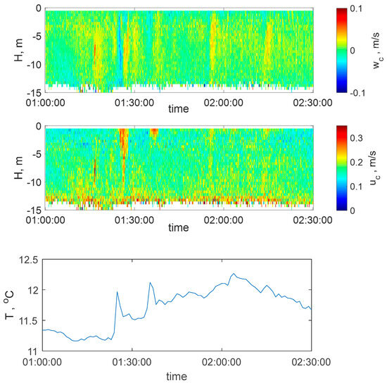
Figure 4.
Vertical (top) and horizontal (bottom) velocity components and water temperature at 0.5 m depth (bottom) for the experiment of 23 May 2019.
The spatial structure of IWs was studied by analyzing a time series of radar images of the sea surface. It is well known that the characteristic features of the IW manifestation on the sea surface, which are observed in the form of bands of alternating roughness, can be related with different IW phases depending on hydrometeorological conditions (see, for example, [13,20]). The time step of radar imaging of the sea surface was 15 s in the experiment. Figure 5 shows radar images of the state of the sea surface obtained in one revolution of the radar antenna. The 330°–60° sector on the radar image is obscured by the platform and excluded from further consideration. The train of IWs is clearly visible in the south of the platform in the form of bands characterized by lower radar cross section (RCS) values (Figure 5a,c,e,g,i,j). Doppler velocity (Figure 5b,d,f,h,j,l) also showed strong variability. Figure 5a,b at 01:09 on 23 May 2023 show the leading soliton (IW1) and the soliton caching up with it (IW2). In Figure 5c,d, at 01:15 on 23 May 2023, the leading soliton (IW1) and the second soliton (IW2) merged. In Figure 5d,f, at 01:19 on 23 May 2023, the second soliton (IW2) passes under the platform. In Figure 5g,h,i,k,l, the interaction of the IW2 soliton with an artificial slick band occurs. In Figure 5k,l, at 01:33 on 23 May 2023, the third soliton (IW3) passes under the platform. The propagation speed of IW solitons was calculated by analyzing the position of such bands on successful radar images (Figure 6b). The area of reduced intensity of surface waves observed in the east of the platform corresponds to an artificial slick band. The IWs propagated from south to north, while the band propagated from west to east. Figure 5b–d,i,k gives a radar image of the Doppler velocity distribution, which clearly shows that surface waves propagate predominantly from west to east; positive Doppler velocity values correspond to the approaching scatterers, and negative values correspond to the retreating ones. In this case, the waves and wind are directed transversely to the direction of IW propagation. Based on a sequence of radar images, one can create a video demonstrating the dynamics of the processes and download it as Supplementary Materials.

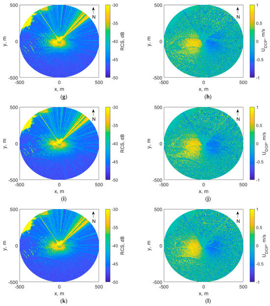
Figure 5.
Radar image of the sea surface on May 23, 2019. RCS at 01:09 (a), 01:15 (c), 01:19 (e), 01:24 (g), 01:29 (i), and 01:33 (k); Doppler velocity at 01:09 (b), 01:15 (d), 01:19 (f), 01:24 (h), 01:29 (j), and 01:33 (l). The x axis is directed to the east and the y axis, to the north; (0,0) is the location of the radar and surfactant source.
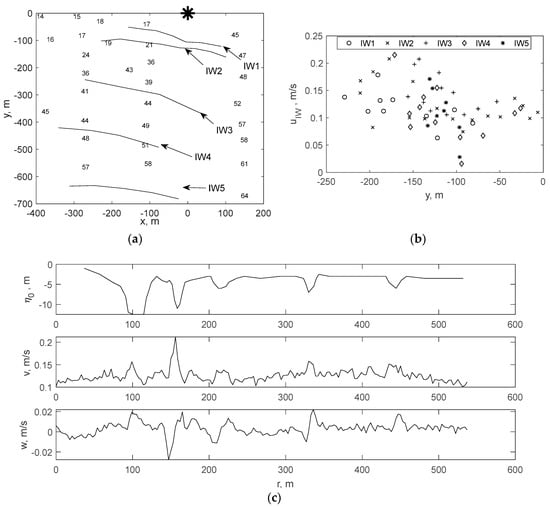
Figure 6.
Spatial structure of the IW-related bands at 1:09 a.m. on 23 May 2019 (a); propagation velocities of individual solitons of the packet (b); amplitudes of the IW solitons, horizontal v and vertical w velocities in a layer of 0.5–12 m during the passage of the IW (c). The numbers show the depth values in meters. The asterisk shows the location of the radar on the platform.
Figure 6a shows the spatial structure of the bands of reduced signal intensity on the radar image at 1:09 on 23 May 2019. The fronts of IW4 and IW5 at this moment had not yet appeared on the radar image, and their location was retrieved using time reversal based on subsequent radar images and calculated propagation velocity (Figure 6b). The numbers in Figure 6a indicate depths in meters. The propagation velocity was calculated from the minimum distance between the positions of the fronts at different times (this can be considered as the lowest estimate of the velocity). The observed slowdown in the propagation of solitons near the platform (Figure 6b) is due probably to a decrease in depth.
Figure 6c shows the spatial distribution of amplitudes and velocity components of the upper-ocean currents containing IW-related currents. It was obtained by converting time into coordinates (r), taking into account the propagation velocity of surface manifestations of IWs near the platform (Figure 6b). Soliton amplitudes are retrieved by determining the position of the maximum intensity gradient of sound backscattering, shown in Figure 3. Current speeds are averaged over the 12 m thick upper layer. It should be noted that the sea depth to the east of the platform is much greater than on the western and southern sides. That is the reason why the IW1 soliton is observed only in one, the fourth ADCP beam, directed exactly to the east (Figure 3). This can also lead to the observed curvature of the IW fronts as they approach the platform. The leading soliton IW1, when approaching the platform, has the largest width among all the solitons in the packet, which may indicate that it has reached the limiting amplitude [21]. Its further transformation and collapse are presumably due to a decrease in the depth of the sea and, accordingly, the depth of the lower layer h2 near the platform. The effective widths of solitons range from 5 to 15 m, the distance between solitons ranges from 30 to 100 m, and the amplitudes of solitons vary from 3 to 10 m.
Based on the analysis of the obtained data, the spatiotemporal characteristics of the passage of solitons near the SOP were retrieved. Since no information about stratification has been collected during the experiment, it is difficult to determine theoretical values of the velocity of soliton propagation. However, it is possible to compare the ratio of amplitudes and half-widths of solitons. The expression for the effective half-width of the Korteweg-de-Vries (KdV) soliton has the form [22]
where is the soliton amplitude. The results of the experimental data analysis and theoretical estimates for the assumptions of two- and three-layer stratification are given in Table 1. The width of the IW1 soliton is shown to have a larger width than both theoretical estimates, indicating that it has reached a critical value and transformed into a Gardner-type soliton [23]. The remaining solitons are characterized by widths close to theoretical estimates for both cases of stratification and can therefore be considered as KdV solitons.

Table 1.
Experimental values and theoretical estimates of the soliton half-widths.
In this section, the parameters of KdV solitons are determined for further study of the transformation of the structure of an artificial slick band in the field of heterogeneous currents related to IW solitons.
3.2. Transformation of an Artificial Slick Band
The kinematics of an extended artificial slick band (ASB) on the sea surface was first studied in [16]. The main factors affecting the width and azimuthal position of the band are current and near-surface wind. Figure 7 shows the speed and direction of the current (uc, ) at a depth of 1 m, as well as the speed and direction of the wind (uw, ) at a height of 24 m during the experiment. For ease of perception, the directions of the current and wind are given in a single coordinate system, so the westerly wind has a direction of about 90 degrees. Based on these data, the speed ud and direction of the surface current were calculated as the vector sum of the current speed and 3% of the wind speed at a standard meteorological height of 10 m [16].
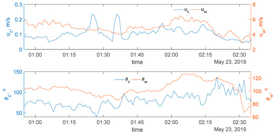
Figure 7.
Speed and direction of the upper-ocean current (at a depth of 1 m) and near-surface wind during the experiment.
The leading soliton IW1, as described above, collapsed on its way to the SOP and did not cause a significant change in the current speed. Although two subsequent solitons IW2 and IW3 had significantly different amplitudes, they caused an increase in the current speed up to 0.25 m/s at a depth of 1 m. Surface currents affecting the ASB dynamics of the ASB can be determined by measuring the Doppler shift of the radar signal from the coherent radar station [20,24]. It should be noted that in the observed case, the direction of IW propagation is perpendicular to the wind; these conditions cannot be considered suitable for measuring surface currents based on Doppler shifts of the radar signal. The cross- wind direction is the most sensitive to changes in wind direction since in this case, the Doppler velocity values change near zero (Figure 5b).
During the passage of the IW packet, strong short-term modulation of the ASB shape was observed in the radar panoramas, which manifested itself in a change in the direction and shape of ASB propagation (Figure 8). The proposed method for processing the results of ASB radar observations is shown in Figure 8b. Each radar image obtained in one revolution of the radar antenna (Figure 8a) provides information about the band boundaries, which can be determined using the maximum brightness gradient condition (Figure 8b). Next, for each vector the slick band fragment is characterized by , where Q is the local angle of the slick fragment in the polar coordinate system, and W is the local band width. Preliminary analysis showed that a spatial resolution of 1 m was sufficient to discern spatial variations of the ASB due to the IW. Previous studies have shown that the effects of surfactant spreading in the band appear on scales of about 100 m from the source [16]. However, in contrast to [16], in the presence of heterogeneous currents from the IW, the film concentration in the ASB cannot be considered constant [13]. According to [13], the inhomogeneity of the concentration depends on the length over which the IW acts on the film.
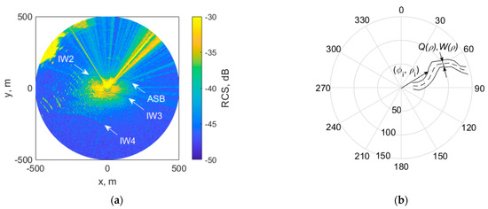
Figure 8.
Radar image of the sea surface during the passage of the IW2 soliton at 01:30 (a) and the scheme of the image processing (b): the solid line depicts the ASB boundaries, and the dotted line is the main direction.
It was noted that changes in the band shape occurred at the moment the IW packet passed the platform, according to the ADCP data and taking into account the difference between the location of the ADCP with an offset from the southern side of the platform and the location of the observation area of the slick band to the east of the platform. Figure 9 shows the results of comparing the direction Q and width W of the ASB at a distance = 100 m from the radar, calculated using the method described in the previous section, with the direction and speed ud of the surface current during the passage of the IW packet. To take into account the spatial difference between the location of the ADCP site and the point characterizing the deformation characteristics of the slick band ( = 100 m), an average time shift of four minutes was used. This value was estimated based on the characteristic propagation velocity of the IW soliton and the described distance of 24 m. It should be noted that there is both qualitative and quantitative consistency between the direction Q of the artificial slick band and the direction of the surface current. The IW2 and IW3 solitons had the greatest effect on the direction of the band, while the IW4 and IW5 solitons manifested themselves only weakly due to their low amplitude. A comparison between the surface current speed and the band width W showed a negative correlation between these values. The observed speed and band width synchronization for IW3 is the result of a random error in determining the time offset between the location of the ADCP and the observation point. Despite this, it appears that the data should be interpreted in the general context of a negative correlation, taking into account the possible small change in the time offset (less than a minute or, accordingly, less than 6 m in space). The introduced time offset of four minutes was the same for all data. Correlation analysis was performed for the direction Q of the ASB and the direction of the surface current, the width W of the band, and the speed ud of the surface current (shown in Figure 9b). The resulting correlation coefficients are 0.8 and −0.44, respectively.
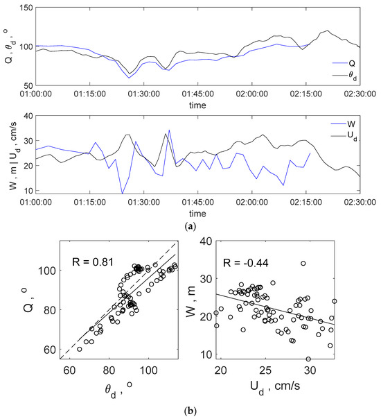
Figure 9.
Comparison of the direction Q and width W of an artificial slick band with the direction , and speed ud of the surface current during the passage of the IW solitons (a). Results of the corresponding correlation analysis (b). R is the correlation coefficient. Solid lines correspond to the linear approximation and the dotted lines to Q = .
To summarize the results of the analysis of experimental data, we can say that the effect of the IW passage on the dynamics of the ASB is manifested in a change in the width W of the band and its direction Q, which can be considered as key parameters characterizing the manifestation of this effect. To interpret observational data and analyze further dynamics of the shape of the slick band in the presence of variable currents, numerical simulation was performed.
3.3. Numerical Simulation Results
To simulate the propagation of surfactants forming a slick band, it is necessary to determine the field of near-surface currents that influence this process. We assumed that the upper-ocean current consists of two components, namely, a constant “background” current, which is affected, among other things, by a wind-wave drift (according to [16]) and a propagating disturbance of the current field induced by an internal wave soliton. To simulate the propagation of surfactants appearing on the water surface from a stationary source, we assume that at each moment of time a marked point appears at the origin of coordinates (0, 0), while the marker with coordinates (x, y) in the Cartesian coordinate system moves in accordance with the local value of the current field. The union of markers represents the shape of the slick band. In the absence of disturbance, the marked points on the surface move along the constant current field. Software permits one to “launch” isolated current field disturbances generated by internal wave solitons in the form
where is the amplitude of the surface current velocity disturbance related to the passage of the internal wave, t is the time, is the phase, is the effective soliton width, and and are unit vectors directed along the Ox and Oy axes, respectively. The wave vector describes the propagation of the disturbance front, is the direction of propagation, and the propagation velocity of the disturbance is described as VIW.
It was shown in [17] that for a slick band formed using a constant surfactant source, the surface concentration of surfactants tends to a constant value at a sufficient distance from the source (more than about 100 m in our conditions). This result is valid when the surface current velocity exceeds the velocity of surfactant propagation over the sea surface. This result also means that each surfactant fragment of a constant volume in the band occupies the same area on the surface when the band is formed. We defined a slick band as a set of individual marked points moving in accordance with the local current velocities. To a first approximation, the occupied area of an individual marker i can be estimated as the product of half the distance between the neighboring points i − 1 and i + 1 and the local width of the band. Based on this condition, the width of the band at point i is inversely proportional to the distance between two neighboring points i − 1 and i + 1. The proportionality coefficient is determined from experimental data based on the values of the undisturbed area’s width and current velocity.
When simulating the case of propagation of the IW2 soliton, we used the following parameters according to experimental data. The background current before the soliton arrival had a value of 23 cm/s and was directed at 86 degrees in the polar coordinate system shown in Figure 8b (mainly to the east). The amplitude of the current speed disturbance related to the soliton was 16.8 cm/s. The speed of soliton disturbance in the north-northeast direction VIW was 12 cm/s. The spatial width of the disturbance was 15 m, and the phase φ = 25. The phase was determined to be minimal based on the fact that by the time the soliton arrives, a band that propagates at the speed of the background current should be formed. The calculation time interval dt = 5 s.
Figure 10 shows the dynamics of propagation of an internal wave soliton and its effect on the shape of an artificial slick band created by a surfactant source placed at the origin of coordinates. The vector field depicted corresponds to the current speeds related to the internal wave soliton.
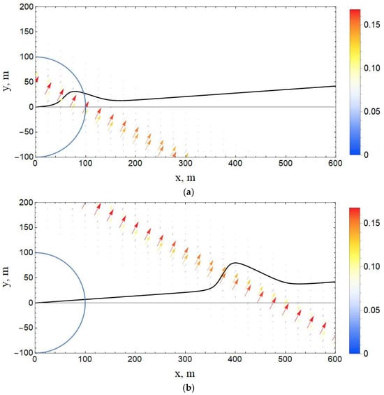
Figure 10.
Dynamics of the slick-band shape during the passage of a current disturbance related to the internal wave soliton. Simulation parameters correspond to the experiment (see the text). (a) t = 1000 s; (b) t = 4800 s. The color bar describes the disturbance modulus of the current speed. A semicircle marks the 100 m area.
In this way, the situation realized in the field experiment was simulated. The calculation results presented in Figure 10a fully simulate IW2 shown in the radar panorama in Figure 8a. Numerical simulation permits one to consider the further spatiotemporal development of the band shape and to study the possible scenarios for the dynamics of the slick band. The soliton propagates with velocity at an angle to the background current Ubackgr and, accordingly, to the undisturbed direction of propagation of the slick band. However, it was clear that the situation could change depending on the relation between Ubackgr cos and . Therefore, simulations with different parameter ratios were performed, and new effects described in the discussion section were discovered.
4. Discussion
A group of passing IWs was studied in field conditions using contact measurements and remote sensing methods. The leading soliton IW1, the most intense in the group, was characterized by a half-width that was 3 times larger than the theoretical estimates for KdV solitons (see Table 1). We assumed that the IW1 soliton was a Gardner soliton that had reached a critical amplitude before the observed collapse. According to the soliton theory [22], the rest of the solitons are classified as KdV solitons. The passage of the remaining solitons, except the collapsed one, led to significant changes in the artificial slick band that was continuously created during the experiment.
To simulate the effect of the passing KdV solitons of internal waves on the shape of the slick band, numerical simulation was performed. The results of simulation and experiment showed good agreement for the local angle of inclination of the band and its width. It should be noted that, since the experimental observation of the band characteristics is limited by the maximum observation range of the radar station and wave parameters, numerical simulation makes it possible to consider the further spatiotemporal development of the band shape and to study possible scenarios for the slick-band dynamics in other conditions.
Simulations have shown that there are three possible scenarios for the dynamics of the slick band due to the relation between Ubackgr cos and .
The condition of a strong background current leads to the situation where the disturbed slick band catches up with the wave front; therefore, the disturbed shape of the slick band can be considered as a precursor of internal waves even before its arrival at the observation area. A similar effect is described in [13].
If , then each element of the slick band which interacted with the field of IW-related currents tends to remain in the wave phase, which corresponds to the condition . This situation describes the effect of the slick band being trapped by the internal wave: all elements of the slick band that are on the sea surface at the time of the soliton arrival drawn near the equilibrium phase, where , and are aligned parallel to the wave front (Figure 11a).
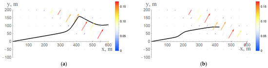
Figure 11.
Possible “opposite” scenarios for the slick-band response to the passage of the internal wave soliton: (a) the slick-band trapping; (b) the “memory” effect.
If , then the rapidly propagating soliton leaves the deformed slick band behind, and then slowly shifts as a whole under the action of the background current. This scenario can be characterized as a “memory” effect of the slick band (Figure 11b).
Based on the results of the experimental data and the corresponding parameters used for the simulation, the observed case corresponds to the precursor scenario. Figure 11 shows the simulation results with some changes in the parameters, which switched the situation to other possible scenarios, namely, the slick-band trapping (Figure 11a, VIW = 19 cm/s) and the “memory” effect (Figure 11b, VIW = 40 cm/s). It should be noted that the described range of current speeds used for the simulation is reasonable as it can be observed in the actual sea environment. Due to the wide range of possible background current speeds Ubackgr, the amplitude of the subsurface current speed generated by internal waves , and the speed of internal wave propagation VIW, all these scenarios can be observed in field conditions [25].
It should be noted that in real conditions, slicks in the coastal area are mainly caused by biogenic films. Subsurface processes, such as internal waves, lead to the redistribution of these slicks, and the location of biogenic slicks may correspond to different phases of the IW [13,26]. Biogenic films are characterized by small concentration disturbances. The ASB is characterized by large concentrations and, although in this case we neglect the internal effects of film dynamics (spreading and relaxation effects) over long distances, it is possible to adequately describe the main kinematic properties of the band. In this case, the soliton phase in which the slick band is trapped is determined by the significant (compared to the disturbance propagation velocity) amplitude of the variable flow induced by the IW soliton. However, it is worth considering that taking into account the internal dynamics of the slick structure can shift this phase. A change in hydrometeorological conditions (drift speed of wind waves or background current) leads to a change in the “equilibrium” phase of the IW, above which the slick is observed. However, even without taking into account these corrections, it is possible, in general, to develop a technique for estimating IW parameters based on changes in the shape of the slick band.
5. Conclusions
A new approach to diagnosing the heterogeneous current speed related to internal waves has been described. Based on the data from field experiments, the spatiotemporal parameters of the internal wave packet are retrieved and the parameters of the artificial slick band, the shape of which responds to disturbances in the horizontal current speed caused by the passage of the internal wave flow, are found. High values of the correlation coefficients between the direction of the upper-ocean current velocity and the direction of the artificial slick band, as well as a negative correlation coefficient between the band width and the magnitude of the upper-ocean current velocity, are shown for the described experimental conditions. Based on the results of numerical simulation of the deformation of a slick band in the field of a heterogeneous current related to internal waves and the data from a field experiment, it is shown that the maximum value of the velocity in the IW soliton can be estimated from the change in shape, direction, and velocity of the internal wave, and that the characteristic spatial scale of the soliton can be determined. The results of the paper indicate the possibility of solving the inverse problem, i.e., determining the parameters of the soliton of internal waves passing through the slick band, which can be observed on optical or radar satellite images of the sea surface. The presence of characteristic deformations (kinks, broadenings, etc.) arising due to the “memory effect” demonstrated during the simulation and the effect of trapping of the existing film deformation may indicate the passage of internal waves and will allow one to evaluate their characteristics.
Supplementary Materials
The following supporting information can be downloaded at: https://www.mdpi.com/article/10.3390/rs16010156/s1, Video S1: video edited from a sequence of radar images during the experiment. All data can be obtained on request.
Author Contributions
Conceptualization, I.K. and A.E.; methodology, I.K. and A.E.; software, O.S.; investigation, A.E., I.K., O.S., A.M., M.S. and N.B.; writing A.E., I.K. and O.S. All authors have read and agreed to the published version of the manuscript.
Funding
This research was funded by the Russian Science Foundation (project No. 18-77-10066) for field research. Doppler radar research and in-depth analysis of the rates of subsurface processes were supported by the Russian Science Foundation (project No. 20-77-10081, https://rscf.ru/project/20-77-10081/, accessed on 1 september 2023).
Data Availability Statement
Data are contained within the article and Supplementary Materials. The calculation data can be provided upon request.
Acknowledgments
The authors thank Olga Danilicheva for her assistance in conducting the experiments, Tatiana Tarasova for help with software, Irina Sergievskaya for valuable comments made during the discussion of the manuscript, and Alexey Krayev for English proofreading.
Conflicts of Interest
The authors declare no conflicts of interest.
References
- Klemas, V. Remote sensing of coastal and ocean currents: An overview. J. Coast. Res. 2012, 28, 576–586. [Google Scholar] [CrossRef]
- Serafino, F.; Lugni, C.; Nieto Borge, J.C.; Zamparelli, V.; Soldovieri, F. Bathymetry Determination via X-Band Radar Data: A New Strategy and Numerical Results. Sensors 2010, 10, 6522–6534. [Google Scholar] [CrossRef] [PubMed]
- Kudryavtsev, V.; Akimov, D.; Johannessen, J.; Chapron, B. On radar imaging of current features: 1. Model and comparison with observations. J. Geophys. Res. 2005, 110, C07016. [Google Scholar] [CrossRef]
- Ardhuin, F.; Gille, S.T.; Menemenlis, D.; Rocha, C.B.; Rascle, N.; Chapron, B.; Gula, J.; Molemaker, J. Small-scale open ocean currents have large effects on wind wave heights. J. Geophys. Res. 2017, 122, 4500–4517. [Google Scholar] [CrossRef]
- Brekke, C.; Espeseth, M.M.; Dagestad, K.-F.; Röhrs, J.; Hole, L.R.; Reigber, A. Integrated analysis of multisensor datasets and oil drift simulations—A free-floating oil experiment in the open ocean. J. Geophys. Res. 2021, 126, e2020JC016499. [Google Scholar] [CrossRef]
- Lipinskaia, N.A.; Salyuk, P.A. Research of the influence of internal waves on the optical characteristics of the sea surface in the shelf zone of Peter the Great Bay. Fund. Appl. Hydrophys. 2020, 13, 51–59. [Google Scholar] [CrossRef]
- Johannessen, J.A.; Kudryavtsev, V.; Akimov, D.; Eldevik, T.; Winther, N.; Chapron, B. On radar imaging of current features: 2. Mesoscale eddy and current front detection. J. Geophys. Res. 2005, 110, C07017. [Google Scholar] [CrossRef]
- Ivanov, A.Y.; Ginzburg, A.I. Oceanic eddies in synthetic aperture radar images. J. Earth Syst. Sci. 2002, 111, 281–295. [Google Scholar] [CrossRef]
- Shomina, O.; Danilicheva, O.; Tarasova, T.; Kapustin, I. Manifestation of Spiral Structures under the Action of Upper Ocean Currents. Remote Sens. 2022, 14, 1871. [Google Scholar] [CrossRef]
- Chapron, B.; Collard, F.; Ardhuin, F. Direct measurements of ocean surface velocity from space: Interpretation and validation. J. Geophys. Res. 2005, 110, C07008. [Google Scholar] [CrossRef]
- Bakhanov, V.V.; Ostrovsky, L.A. Action of strong internal solitary waves on surface waves. J. Geophys. Res. 2002, 107, 3139. [Google Scholar] [CrossRef]
- Ermakov, S.A.; Salashin, S.G. On strong modulation of capillary-gravitational ripples by internal waves. Dokl. Acad. Sci. USSR 1994, 337, 108–111. [Google Scholar]
- Ermakov, S.A. Vliyanie Plenok na Dinamiku Gravitatsionno-Kapillyarnykh voln (Impact of Surfactant Films on the Dynamics of Gravity-Capillary Waves), 1st ed.; IAP RAS: Nizhny Novgorod, Russia, 2010; pp. 89–162. [Google Scholar]
- Sabinin, K.D.; Lavrova, O.Y. Impact of internal soliton interaction on surface manifestation of ship wakes. Sovrem. Probl. Distantsionnogo Zondirovaniya Zemli Iz Kosmosa 2011, 8, 256–262. [Google Scholar]
- Kozlov, I.E.; Zubkova, E.V.; Kudryavtsev, V.N. Internal Solitary Waves in the Laptev Sea: First Results of Spaceborne SAR Observations. IEEE Geosci. Remote Sens. Lett. 2017, 14, 2047–2051. [Google Scholar] [CrossRef]
- Kapustin, I.A.; Shomina, O.V.; Ermoshkin, A.V.; Bogatov, N.A.; Kupaev, A.V.; Molkov, A.A.; Ermakov, S.A. On Capabilities of Tracking Marine Surface Currents Using Artificial Film Slicks. Remote Sens. 2019, 11, 840. [Google Scholar] [CrossRef]
- Shomina, O.V.; Kapustin, I.A.; Ermoshkin, A.V.; Ermakov, S.A. On the dynamics of artificial slick band in the coastal zone of the Black Sea. Sovrem. Probl. Distantsionnogo Zondirovaniya Zemli Iz Kosmosa 2019, 16, 222–232. [Google Scholar] [CrossRef]
- Carr, M.; Davies, P.A. The motion of an internal solitary wave of depression over a fixed bottom boundary in a shallow, two-layer fluid. Phys. Fluids 2006, 18, 016601. [Google Scholar] [CrossRef]
- Semin, S.; Kurkina, O.; Kurkin, A.; Talipova, T.; Pelinovsky, E.; Churaev, E. Features of fluid flows in strongly nonlinear internal solitary waves. Nonlinear Process. Geophys. Discuss. 2014, 1, 1919–1946. [Google Scholar] [CrossRef]
- Kropfli, R.A.; Ostrovski, L.A.; Stanton, T.P.; Skirta, E.A.; Keane, A.N.; Irisov, V. Relationships between strong internal waves in the coastal zone and their radar and radiometric signatures. J. Geophys. Res. 1999, 104, 3133–3148. [Google Scholar] [CrossRef]
- Gorshkov, K.A.; Soustova, I.A.; Ermoshkin, A.V.; Zaytseva, N.V. Evolution of the compound Gardner-equation soliton in the media with variable parameters. Radiophys. Quantum Electron. 2012, 55, 344–355. [Google Scholar] [CrossRef]
- Ostrovsky, L.A.; Stepanyants, Y.A. Internal solitons in laboratory experiments. Comparison with theoretical models. Chaos 2005, 15, 037111. [Google Scholar] [CrossRef] [PubMed]
- Gorshkov, K.A.; Soustova, I.A.; Ermoshkin, A.V. Field Structure of a Quasisoliton Approaching the Critical Point. Radiophys. Quantum Electron. 2016, 58, 738–744. [Google Scholar] [CrossRef]
- Ermoshkin, A.V.; Kapustin, I.A.; Molkov, A.A.; Bogatov, N.A. Determination of the sea surface current by a Doppler X-band radar. Fundam. Prikl. Gidrofiz. 2020, 13, 93–103. [Google Scholar] [CrossRef]
- Sabinin, K.D.; Serebryany, A.N. “Hot spots” in the field of internal waves in the ocean. Acoust. Phys. 2007, 53, 357–380. [Google Scholar] [CrossRef]
- Ewing, G. Slicks, surface films and internal waves. J. Mar. Res. 1950, 9, 161–187. [Google Scholar]
Disclaimer/Publisher’s Note: The statements, opinions and data contained in all publications are solely those of the individual author(s) and contributor(s) and not of MDPI and/or the editor(s). MDPI and/or the editor(s) disclaim responsibility for any injury to people or property resulting from any ideas, methods, instructions or products referred to in the content. |
© 2023 by the authors. Licensee MDPI, Basel, Switzerland. This article is an open access article distributed under the terms and conditions of the Creative Commons Attribution (CC BY) license (https://creativecommons.org/licenses/by/4.0/).