Technical Note

Enhanced Micro-Doppler Feature Extraction Using Adaptive Short-Time Kernel-Based Sparse Time-Frequency Distribution

College of Electronic Science and Technology, National University of Defense Technology, Changsha 410073, China
*
Author to whom correspondence should be addressed.
Remote Sens. 2024, 16(1), 146; https://doi.org/10.3390/rs16010146
Submission received: 9 November 2023 / Revised: 12 December 2023 / Accepted: 27 December 2023 / Published: 29 December 2023
(This article belongs to the Special Issue Doppler Radar: Signal, Data and Applications)

Abstract

:
The extraction of the micro-Doppler (m-D) feature based on time-frequency distribution (TFD) is of great significance for target detection and identification. To improve the feature extraction performance, numerous TFDs have been developed, with the majority falling under Cohen’s class. Nevertheless, these TFDs basically face a trade-off between artifact suppression and energy concentration. The main reason is that each Cohen’s class TFD is constructed by applying the two-dimensional Fourier transform to a kerneled ambiguity function directly, while existing kernels generally attenuate artifacts at the expense of losing valuable information. In this paper, a TFD reconstruction method employing an adaptive short-time kernel (ASTK) is developed in the framework of sparse representation (SR) theory to overcome this trade-off and enhance the m-D feature. Firstly, the task of the optimal kernel is explained from the viewpoint of the instantaneous auto-correlation function (IAF). Secondly, based on the quasi-linear frequency modulation feature of most m-D signals during short-time periods, the distribution rule of the short-time IAF (STIAF) in the ambiguity plane is concluded. Guided by this rule, an ASTK that can effectively remove unwanted artifacts with the least information loss is designed. Finally, an SR-based reconstruction procedure is conducted on the kerneled STIAF to generate an artifact-free TFD with high energy concentration, which can effectively enhance the m-D feature. Experiments using both simulated and real-world m-D signals demonstrate the effectiveness of the proposed method.

Graphical Abstract

1. Introduction

Micro-motions refer to the small-amplitude movements of radar targets or structures on the targets, in addition to the bulk motion. Micro-motions are commonly observed in the real world, such as the vibrations of a vehicle engine, the rotation of helicopter rotor blades, or the tumbling of a spacecraft in space [1]. From the perspective of radar, these micro-motions can cause unique frequency modulations in the radar echo, resulting in the generation of sidebands around the target’s Doppler frequency shift. This phenomenon is known as the micro-Doppler (m-D) effect.
In recent years, the value of the m-D feature as one of the most significant target signatures has been confirmed. On the one hand, the m-D feature enables the differentiation between targets and backgrounds, which can effectively aid target detection [2,3]. On the other hand, the m-D modulation parameters such as repetition period and maximum amplitude indicate the motion or physical properties of the target, which provides valuable additional information for precise target detection and identification [3,4,5]. Numerous algorithms have been developed to analyze and extract the m-D feature from radar measurements, among which the time-frequency distribution (TFD) has garnered significant attention [6]. The TFD is capable of visualizing the frequency content of an m-D signal over time, thus enabling a clear display of intricate time-varying m-D modulation information of the target. In [7], the Short-Time Fourier Transform (STFT) was utilized to reveal the m-D feature of rotationally symmetric ballistic targets with precession. In [8], radar measurements of diverse targets including humans, vehicles, dogs, and sheep were processed and compared using STFT. Marple proposed time-frequency sharpening techniques to extract the m-D characteristics of helicopter echo signals, which further supported the accurate classification of four-blade and two-blade helicopters [9,10]. In the analysis of human gait echoes, researchers pointed out that extracting the m-D feature from the low-resolution TFD generated by STFT is technically challenging since m-D modulation curves corresponding to different parts of the body overlap with each other. However, using the high-resolution TFD obtained by the reassignment method allows for a clear distinction of the m-D from nine different parts of the human body [11,12]. Therefore, it is crucial to employ a TFD with high energy concentration for the precise extraction of a target’s m-D feature.
At first glance, the Wigner-Ville distribution (WVD) may stand out as one of the most appealing options in m-D feature extraction because it is well-known that WVD has excellent TF concentration, particularly for mono-component linear frequency modulation (LFM) signals. However, as a quadratic TFD, WVD produces desired auto-terms (ATs) and unwanted artifacts simultaneously. To be more specific, the artifacts comprise inner and outer artifacts (commonly referred to as cross-terms), which are induced by the nonlinear frequency modulation (FM) characteristic and the multi-component nature of the signal, respectively [13,14]. Generally, the complex micro-motions of targets cause time-varying frequency modulations in the radar echo, and the observation scene rarely consists of a single target. As a result, the presence of artifacts in WVD is almost inevitable. These artifacts significantly obscure the target’s m-D information, thereby reducing the readability and practicality of WVD in m-D analysis [15,16].
Quantities of modified versions of WVD have been proposed to remove or at least attenuate artifacts, most of which can be categorized under Cohen’s class [17]. Based on the fact that ATs mainly cluster near the origin in the ambiguity plane, while artifacts tend to lie farther away from it [18,19], each member of Cohen’s class involves applying a low-pass kernel to the signal’s ambiguity function (AF) and then obtaining an artifact-suppressed TFD by taking the two-dimensional (2-D) Fourier transform (FT) of the weighted AF. Obviously, the performance of such a TFD relies heavily on the choice of the kernel.
So far, various kernels have been proposed according to the aforementioned distribution pattern of the AF [20,21,22,23,24,25,25]. However, existing kernels, including the well-known adaptive optimal kernel (AOK) [23], face a trade-off between AT preservation and artifact excision. The cause of this issue is that the words “near” and “farther” used to differentiate ATs and artifacts are inherently vague, and thus cannot provide precise guidance for kernel design. Moreover, applying a crude Fourier inversion to the kerneled AF without any constraint tends to reduce the energy concentration [26]. Consequently, the performance of Cohen’s class TFDs is fundamentally limited.
Inspired by the local quasi-LFM feature of most real-life signals [27,28,29], this paper proposes an effective TFD reconstruction approach to generate high-performance TFDs of radar echoes to enhance the target’s m-D characteristic. The main contributions are as follows.
  • An explicit distribution rule of the signal’s short-time AF (STAF) is derived, providing a clear explanation of a phenomenon that was vaguely described in previous literature.
  • The task of the optimal kernel is analyzed and clearly illustrated. Moreover, an adaptive short-time kernel (ASTK) is developed according to the concluded distribution rule, which achieves excellent artifact removal and accurate AT preservation simultaneously.
  • A sparse representation (SR)-based reconstruction method for the instantaneous spectrum is proposed, which further facilitates the construction of an artifact-free TFD with high energy concentration to enhance the m-D characteristic.
This paper is organized as follows. In Section 2, the task of the optimal kernel is analyzed and the ASTK is derived based on the ambiguity domain distribution pattern of the m-D signal’s STIAF. Following this, the reconstruction process of the proposed high-performance TFD is detailed. Section 3 compares the proposed TFD with four other methods using simulated and real m-D signals to demonstrate its superiority. Finally, Section 4 presents conclusions and outlines future research directions.

2. Proposed M-D Feature Enhancement Method

2.1. Task of Optimal Kernel

In general, an m-D signal and its idealized TFD can be respectively represented as [30]
s ( t ) = k = 1 K s k ( t ) = k = 1 K a k ( t ) e j φ k ( t ) ,
P ideal ( t , ω ) = k = 1 K a k 2 ( t ) δ ω φ k ( t ) ,
where K is the number of signal components, s k ( t ) denotes the k-th component with time-varying amplitude a k ( t ) , phase φ k ( t ) , δ ( · ) represents the Dirac delta function, and φ k ( t ) stands for the first order derivative of φ k ( t ) . Conceptually, TFDs in Cohen’s class are generated. All integrals run from to unless otherwise noted.
P ( t , ω ) = 1 4 π 2 A ( θ , τ ) Φ ( θ , τ ) e j θ t j τ ω d θ d τ ,
where A ( θ , τ ) is the AF of s ( t ) , Φ ( θ , τ ) denotes the TFD kernel, θ and τ signify the Doppler frequency and the correlation lag, respectively. More specifically, A ( θ , τ ) is given by
A ( θ , τ ) = R ( t , τ ) e j θ t d t ,
where R ( t , τ ) stands for the instantaneous auto-correlation function (IAF) of s ( t ) , which is expressed as
R ( t , τ ) = s ( t + τ 2 ) s * ( t τ 2 ) ,
( · ) * represents the conjugate operator.
By comparing (2) and (3), it can be observed that if A ( θ , τ ) Φ ( θ , τ ) can be replaced by 2 π k = 1 K a k 2 ( t 1 ) e j φ k ( t 1 ) τ e j θ t 1 d t 1 , we have
P ( t , ω ) = 1 4 π 2 A ( θ , τ ) Φ ( θ , τ ) e j θ t j τ ω d θ d τ = 1 4 π 2 2 π k = 1 K a k 2 ( t 1 ) e j φ k ( t 1 ) τ e j θ t 1 d t 1 e j θ t j τ ω d θ d τ = 1 2 π k = 1 K a k 2 ( t 1 ) e j φ k ( t 1 ) τ e j θ t 1 d t 1 e j θ t d θ e j τ ω d τ = k = 1 K a k 2 ( t ) e j φ k ( t ) τ e j τ ω d τ = k = 1 K a k 2 ( t ) δ ω φ k ( t )
That is to say, Cohen’s class TFD can be transformed into the idealized TFD under the condition of (6). Therefore, the optimal kernel is supposed to be
Φ opt ( θ , τ ) = k = 1 K a k 2 ( t ) e j φ k ( t ) τ e j θ t d t R ( t , τ ) e j θ t d t ,
where the amplitude of the kernel is neglected.
Expanding φ k ( t + τ 2 ) and φ k ( t τ 2 ) into Taylor series at t, we have
φ k ( t + τ 2 ) = φ k ( t ) + φ k ( t ) · τ 2 + φ k ( t ) 2 ! · ( τ 2 ) 2 +
φ k ( t τ 2 ) = φ k ( t ) + φ k ( t ) · ( τ 2 ) + φ k ( t ) 2 ! · ( τ 2 ) 2 +
where φ k ( t ) stands for the second order derivative of φ k ( t ) .
Substituting (1) as well as (8) and (9) into (5), R ( t , τ ) can be expanded as
R ( t , τ ) = k = 1 K R k k ( t , τ ) + k = 1 K l = 1 , l k K R k l ( t , τ )
where R k k ( t , τ ) represents the IAF of s k ( t ) and R k l ( t , τ ) represents the instantaneous cross-correlation function (ICF) between s k ( t ) and s l ( t ) as the l-th component of the m-D signal. R k k ( t , τ ) and R k l ( t , τ ) are respectively given by
R k k ( t , τ ) = s k ( t + τ 2 ) s k * ( t τ 2 ) = a k 2 ( t ) e j φ k ( t + τ 2 ) φ k ( t τ 2 ) a k 2 ( t ) e j φ k ( t ) τ + m = 1 φ k ( 2 m + 1 ) ( t ) ( 2 m + 1 ) ! · 2 2 m τ ( 2 m + 1 ) high-order-derivative terms
R k l ( t , τ ) = s k ( t + τ 2 ) s l * ( t τ 2 ) = a k ( t ) a l ( t ) e j φ k ( t + τ 2 ) φ l ( t τ 2 )
In (11) and (12), the amplitude of each component is assumed to vary slowly, and thus a k ( t ± τ 2 ) = a k ( t ) . φ k ( 2 m + 1 ) ( t ) stands for the ( 2 m + 1 ) order derivatives of φ k ( t ) .
Referring to (7)–(12), the task of the optimal kernel can be more precisely interpreted. In essence, Φ opt ( θ , τ ) aims to eliminate the R k l ( t , τ ) as well as the high-order-derivative terms within each R k k ( t , τ ) in the ambiguity domain. This is because the former introduces outer artifacts while the latter contributes to the inner artifacts. However, designing such a kernel poses a technical challenge because it is still unclear how to accurately differentiate the terms that should be captured from the others that need to be excluded. The remainder of this section presents a practical scheme.

2.2. Distribution Rule of STIAF in Ambiguity Domain

In fact, a more explicit distribution rule for each term in R ( t , τ ) can be derived with the idea of local signal processing. A t 0 -centered short-time m-D signal is represented as
s t 0 ( t ) = s ( t ) w ( t t 0 ) ,
where w ( t ) is a symmetrical window function with length L, i.e., w ( t ) 0 only for t [ L 2 , L 2 ] . In this paper, w ( t ) is set to be a rectangular window.
With a proper value of L, s t 0 ( t ) can be precisely approximated as the superposition of K LFM components, which is exactly the local quasi-LFM feature commonly observed in real-life signals [27,28,29]. In this case, if we expand each phase function into the corresponding Taylor series at t 0 , all terms higher than the second can be omitted. That is,
s t 0 ( t ) k = 1 K a k ( t ) e j x k t 2 + y k t + z k LFM signal , t [ t 0 L 2 , t 0 + L 2 ] ,
where x k = φ k ( t 0 ) / 2 , y k = ( φ k ( t 0 ) φ k ( t 0 ) t 0 ) , z k = φ k ( t 0 ) φ k ( t 0 ) t 0 + φ k ( t 0 ) 2 t 0 2 . Similarly, for the l-th component of s t 0 ( t ) , x l = φ l ( t 0 ) / 2 , y l = ( φ l ( t 0 ) φ l ( t 0 ) t 0 ) , z l = φ l ( t 0 ) φ l ( t 0 ) t 0 + φ l ( t 0 ) 2 t 0 2 .
The AF of s t 0 ( t ) , i.e., the short-time AF (STAF) of s ( t ) , is defined as
A t 0 ( θ , τ ) = R t 0 ( t , τ ) e j θ t d t ,
where R t 0 ( t , τ ) stands for s ( t ) ’s short-time IAF (STIAF) and is expressed as
R t 0 ( t , τ ) = s t 0 ( t + τ 2 ) s t 0 * ( t τ 2 ) = k = 1 K R t 0 , k k ( t , τ ) + k = 1 K l = 1 , l k K R t 0 , k l ( t , τ ) ,
R t 0 , k k ( t , τ ) and R t 0 , k l ( t , τ ) represent the time-localized version of R k k ( t , τ ) and R k l ( t , τ ) , respectively. The range of t is [ t 0 L 2 , t 0 + L 2 ] , while τ is limited in [ L , L ] .
Using (14), R t 0 , k k ( t , τ ) and R t 0 , k l ( t , τ ) can be obtained as
R t 0 , k k ( t , τ ) a k 2 ( t ) e j ( 2 x k t + y k ) τ = e j φ k ( t 0 ) + φ k ( t 0 ) ( t t 0 ) τ
R t 0 , k l ( t , τ ) a k ( t ) a l ( t ) e j ( x k l t 2 + y k l t + z k l )
where x k l = x k x l , y k l = ( x k + x l ) τ + y k + y l , z k l = ( x k x l ) τ 2 4 + ( y k y l ) τ 2 + z k z l .
For variable t, R t 0 , k k ( t , τ ) in (17) is a narrow-band single-frequency signal with constant frequency 2 x k τ and initial phase y k τ , but R t 0 , k l ( t , τ ) in (18) is a wide-band LFM signal with chirp rate 2 x k l , initial frequency y k l , and initial phase z k l . Since STAF is exactly the inverse FT of STIAF with respect to t, for each value of τ , the energy of R t 0 , k k ( t , τ ) is highly concentrated in the ambiguity domain, whereas the energy of R t 0 , k l ( t , τ ) disperses across its instantaneous bandwidth. Considering all values of τ , a more explicit distribution pattern in the ambiguity plane can be derived.
If the signal’s frequency exhibits approximately linear variation, the energy of auto-terms is distributed along lines passing through the origin, while the energy of artifacts is dispersed within a diamond-shaped region.
To illustrate the above conclusion, Figure 1 shows the STAF of a two-component LFM signal and the corresponding cross-section at τ = 0.5 s. The LFM signal is expressed as
s 1 ( t ) = e j 100 π t + 200 π t 2 + e j 100 π t 200 π t 2 .
Through an inspection of the results shown in Figure 1, the correctness of the concluded distribution rule can be verified. It is worth noting that the prerequisite for applying this rule is the quasi-LFM feature of the short-time signal. Hence, the analysis window is supposed to break down the original m-D signal into a series of short-time segments with linearly varying frequencies. To achieve this, the adaptive window proposed in [27] is employed, which is generated through the minimization of the bandwidth of each short-time signal. The reason is that the more stationary the short-time signal, the slower its frequency varies, leading to a smaller bandwidth of the short-time signal. Therefore, it is reasonable to consider the bandwidth of each short-time signal as an indicator of LFM approximation precision. A smaller bandwidth indicates higher approximate precision.

2.3. ASTK Design

By comparing (11) and (17), it is apparent that the high-order-derivative terms within each R k k ( t , τ ) are absent in its time-localized counterpart R t 0 , k k ( t , τ ) . Therefore, the primary objective of the short-time kernel for s t 0 ( t ) shifts toward the suppression of R t 0 , k l ( t , τ ) . Based on the STIAF’s distribution rule concluded in Section 2.2, if we accumulate the energy of the STAF through lines passing through the origin as
E ( α ) = 0 A t 0 ρ cos α , ρ sin α d ρ , α [ 0 , 2 π ) ,
energy peaks can be obtained in the directions that each R t 0 , k k ( t , τ ) is distributed along, while the energy of each R t 0 , k l ( t , τ ) cannot be effectively accumulated from any angle. In (20), E ( α ) denotes the accumulated energy along a line passing through the origin with an inclination angle of α , and ρ represents the polar radius. Prior to the energy accumulation, an interpolation of the STAF from the rectangular grid to the polar grid is necessary. A detailed description of the interpolation process can be found in [24].
Finally, the ASTK can be derived by assigning the value of 1 to directions that correspond to the energy peaks while maintaining 0 for all other locations. As a result, the shape of the kernel is dynamically determined through the energy accumulation procedure, allowing it to adaptively adjust to match various short-time signals. For example, an X-shaped kernel will be derived for the STAF shown in Figure 1. Using this kernel, each R t 0 , k l ( t , τ ) can be effectively removed while each R t 0 , k k ( t , τ ) is precisely preserved. As a result, we have
r t 0 ( t , τ ) = F θ t { A t 0 ( θ , τ ) Φ t 0 ( θ , τ ) } k = 1 K R t 0 , k k ( t , τ ) k = 1 K a k 2 ( t ) e j φ k ( t 0 ) + φ k ( t 0 ) ( t t 0 ) τ
where r t 0 ( t , τ ) stands for the kerneled STIAF, t is limited in [ t 0 L 2 , t 0 + L 2 ] , F θ t denotes the FT from Doppler frequency θ to time t.

2.4. SR-Based TFD Reconstruction

Traditionally, once r t 0 ( t , τ ) is determined, the instantaneous spectrum at time instant t 0 can be computed as [24]
P ( t 0 , ω ) = F τ ω { r t 0 ( t 0 , τ ) } = F τ ω k = 1 K a k 2 ( t 0 ) e j φ k ( t 0 ) τ .
where F τ ω denotes the FT from correlation lag τ to frequency ω .
By continuously sliding the analysis window and computing the spectrum for each time instant, an artifact-suppressed TFD (called ASTK-FT TFD hereafter) can be generated by arranging the obtained spectrums chronologically. However, since the range of τ for each r t 0 ( t , τ ) is limited by the length of the short-time signal, the concentration of each instantaneous spectrum is usually unsatisfactory due to the uncertainty principle [22]. Hence, ASTK-FT TFD still inherits poor energy concentration.
Since K is usually a small number in practice, the signal’s inherent sparsity can be utilized to generate “sharper” spectrums [31,32]. By employing a l 0 norm sparsity constraint, the sparse spectrum at time instant t 0 can be computed as
P ^ ( t 0 , ω ) = arg min P ( t 0 , ω ) P ( t 0 , ω ) 0 s . t . F τ ω 1 { P ( t 0 , ω ) } = r t 0 ( t 0 , τ )
where · 0 signifies the l 0 norm, and F τ ω 1 stands for the inverse FT from frequency ω to correlation lag τ .
It is well-known that sparse representation problems based on the l 0 norm are NP-hard. In this paper, an effective sparse decomposition algorithm named SL0 is utilized to solve (23). The SL0 algorithm uses the smoothed l 0 norm to find sparse solutions and has been verified to perform even faster than l 1 -norm-based algorithms [33]. The SL0 algorithm has been successfully used in time-frequency analysis and behaves well. Readers can refer to [34] for more details about the process of the SL0 algorithm for instantaneous spectrum reconstruction.
By combining the effective ASTK and SR-based spectrum reconstruction procedure, the desired high-performance TFD (named ASTK-SR TFD) can be derived. The proposed TFD differs from AOK TFD in three aspects. First, ASTK-SR TFD employs an adaptive window to decompose the signal into short-time segments, whereas the AOK TFD uses a fixed window. Secondly, ASTK-SR TFD devises an adaptive kernel to weigh the signal’s STAF, while the AOK TFD utilizes low-pass kernels with Gaussian radial cross sections. Lastly, ASTK-SR TFD utilizes SR techniques to construct the spectrum, whereas the AOK TFD relies on the Fourier transform. To conclude, the complete signal processing process of the proposed method is illustrated in Figure 2 and summarized as follows.
  • Break the m-D signal to be analyzed into a series of short-time segments with the adaptive window.
  • Compute the STAF of each short-time signal in both rectangular and polar coordinates.
  • Accumulate the STAF energy along lines passing through the origin with different slopes to determine the shape of the ASTK.
  • Apply the ASTK to the STAF to suppress unwanted artifacts.
  • Take inverse FT to the kerneled STAF to obtain the artifact-free STIAF.
  • Reconstruct the instantaneous spectrum by utilizing the sparsity of the STIAF slice in the corresponding Fourier dictionary.
  • Obtain the high-performance TFD by arranging the spectrums of all time instants chronologically.

3. Experimental Results and Analysis
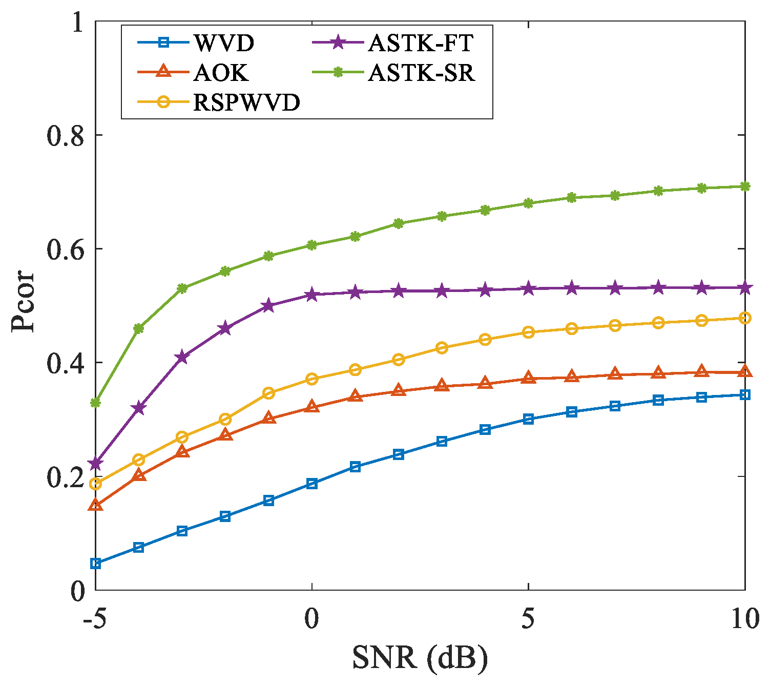
In this section, synthetic and real-life m-D signals are employed to demonstrate the superiority of the proposed ASTK-SR TFD in m-D feature enhancement. To provide a comprehensive comparison, WVD, which is one of the most well-known methods with excellent energy concentration, and RSPWVD, which is known to usually behave best in practical applications, are chosen as benchmarks in all comparisons. Moreover, since AOK TFD shares similar ideas and signal processing procedures with the proposed method, it is also included in the following experiments. Finally, the results of ASTK-FT TFD are also provided to demonstrate the benefit introduced by the SR technique.

3.1. Simulation

Tumbling refers to a type of complex micro-motion that consists of rotation, translation, and acceleration. Using the theoretical model deduced in [1], the radar return of a tumbling target composed of three ideal scatterers is computed. The simulation parameters are listed in Table 1.
The theoretical m-D feature of the simulated radar echo and five considered TFDs computed with a 0 dB signal-to-noise ratio (SNR) are depicted in Figure 3 for a visual comparison of their energy concentration and artifact suppression ability. For a more comprehensive comparison, the cross-sections of these TFDs at time = 0.5 s are also depicted in Figure 4. As the performance of AOK TFD relies on the kernel volume parameter [23] and RSPWVD is dependent on the choice of window lengths [30], experiments have been conducted with various parameters. The TFDs reported in Figure 3 have all been individually optimized to be the most visually appealing outcome for a fair and unbiased comparison.
As shown in Figure 3, WVD is seriously contaminated by artifacts and noise due to the lack of interference suppression ability, while the others significantly reduce artifacts. However, AOK TFD fails to provide a clear TF image due to the limited artifact suppression ability provided by the radially Gaussian kernel. Furthermore, the TF trajectories are heavily expanded as numerous AF data related to ATs have been deserted. By assigning the dispersed TF energy back to the center of gravity at each time instant, RSPWVD truly improves the energy concentration. On the other hand, it still encounters the same issue of residual artifacts as AOK TFD does. Moreover, RSPWVD is very sensitive to noise, and thus the obtained TF trajectories are slightly twisted. Due to the advanced capabilities of the proposed ASTK in attenuating artifacts and noise while accurately preserving ATs’ information, ASTK-FT TFD is able to distinctly reveal the target’s m-D characteristic. However, as evidenced by Figure 4, the TF trajectories are still widened due to the employment of the 2-D FT. By combining the strengths of SR and ASTK, the proposed ASTK-SR TFD effectively suppresses artifacts and maintains high TF concentration, which closely resembles the theoretical TFD and thus achieves the most accurate m-D feature expression among the methods under consideration.
To quantitatively measure the performance of different TFDs, the Pearson correlation coefficients between them and the theoretical TFD are computed as
Pcor = vec ( P ^ ) T vec P ideal vec ( P ^ ) 2 vec P ideal 2
where P ^ stands for the TFD generated by a certain method, vec ( P ^ ) represents the vector form of P ^ with the mean value subtracted, ( · ) T denotes the vector transpose operation, and · 2 is the l 2 norm. The Pearson correlation can measure the similarity in shape between the computed TFDs and the theoretical TFD and a higher value means better shape similarity [32]. Conceptually, a value of 1 indicates an excellent match with the signal’s time-frequency feature, in other words, the most precise extraction of the target’s m-D feature.
The Pearson correlations between the results and the standard distribution are computed in Table 2. From a closer inspection of the data, it is evident that the correlation coefficients for WVD, AOK TFD, and RSPWVD are all below 0.5. In contrast, notably higher values can be observed for ASTK-FT TFD and ASTK-SR TFD, which confirms the effectiveness of the ASTK and highlights the superiority of ASTK-SR TFD over the other methods.
Moreover, to explore the performance of these TFDs in noise tolerance, white Gaussian noise is added to the synthetic m-D signal to simulate different SNRs varying from −5 dB to 10 dB. At each SNR, 100 Monte-Carlo trials are conducted to obtain the average Pearson correlation coefficients of different methods. As shown in Figure 5, one can see that all TFDs experience a performance deterioration as the SNR decreases. However, the proposed ASTK-SR TFD and ASTK-FT TFD always have much higher correlation coefficients with the theoretical TFD. The two ASTK-based methods show better noise robustness because the noise is randomly distributed in the ambiguity domain, and thus can be effectively filtered by the well-designed ASTK. Taken together, the overall assessment is that the proposed ASTK-SR TFD behaves better in energy concentration, artifact suppression, precision, and noise robustness among all the considered TFDs.

3.2. Computational Complexity
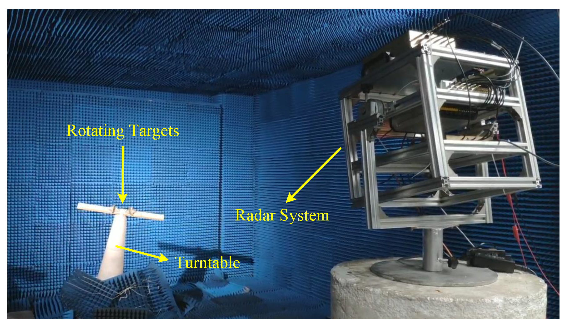
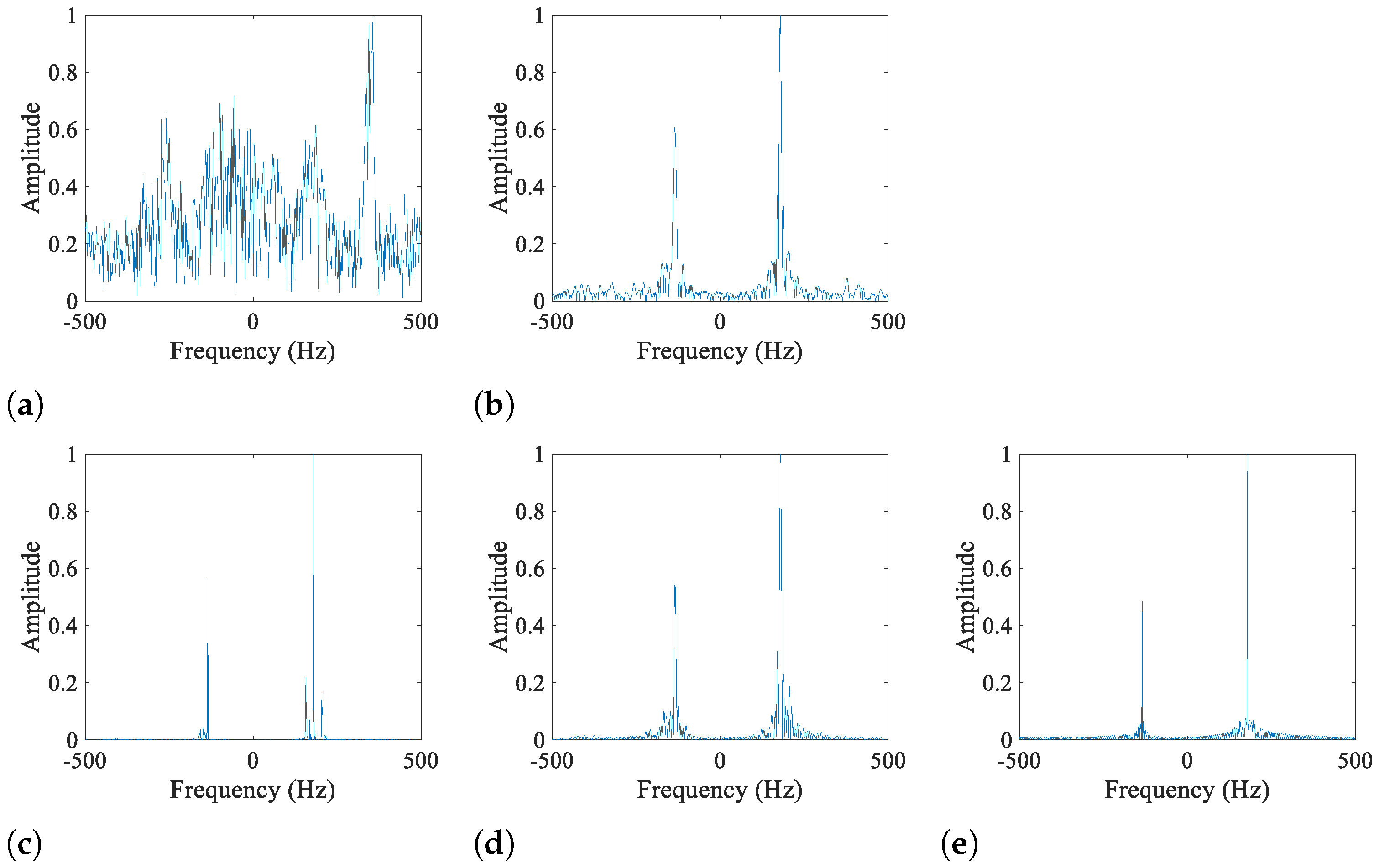
In this subsection, the five considered TFDs are compared from a computational viewpoint.
Assume an N-point sampled m-D signal whose TFD is supposed to be computed over N frequency bins. As previously mentioned, the reconstruction of the proposed ASTK-SR TFD can be summarized into seven steps. From a computational perspective, the cost of steps one and seven can be omitted. For step two, assuming the average length of the short-time window is L ¯ , the dimension of each STAF in rectangular coordinate is L ¯ × L ¯ and can be obtained by L ¯ FFT procedures of size L ¯ . Therefore, the computation of N STAFs in rectangular coordinates requires O ( N L ¯ 2 l o g L ¯ ) operations. Bilinear interpolation is an effective method for calculating the STAF in polar coordinates. The proposed method sets the dimension of the STAF in polar coordinates to be 2 L ¯ × 2 L ¯ , which means that it takes O ( L ¯ 2 ) operations to generate it from a rectangularly sampled STAF. Therefore, the cost of computing N STAFs in polar coordinates is O ( N L ¯ 2 ) . To sum up, the total computational cost of step two is O ( N L ¯ 2 l o g L ¯ ) . For step three, the energy accumulation in each direction is simply achieved by 2 L ¯ additions. Consequently, the cost of energy accumulation in 2 L ¯ angles is O ( L ¯ 2 ) , which means the complexity of the determination of N adaptive kernels is O ( N L ¯ 2 ) . For step four, each rectangularly sampled STAF is multiplied by the corresponding adaptive kernel, requiring O ( N L ¯ 2 ) operations in total. The transformation from each STAF to STIAF involves L ¯ FFT procedures of size L ¯ . Therefore, the computational cost of step five is O ( N L ¯ 2 l o g L ¯ ) . It has been derived that the computational cost of the SL0 algorithm is O U 2 N for a U × N dictionary matrix [34]. As a result, the generation of N instantaneous spectrums in step six needs O ( N 2 L ¯ 2 ) operations since the average size of the adaptive Fourier dictionaries is L ¯ × N . To be more intuitive, the computational cost of the main steps of the proposed method is listed in Table 3.
Summing all data in Table 3, the computational complexity of the reconstruction of ASTK-SR TFD can be derived as O ( N 2 L ¯ 2 ) . Since the ASTK-FT TFD differs from ASTK-SR TFD only by using FFT to construct the spectrum in step six and the N FFT procedures require O ( N 2 l o g N ) operations, the computational cost of ASTK-FT TFD can be obtained as O ( N L ¯ 2 l o g L ¯ ) .
After consulting relevant literature [23,30,34], the computational complexities of the five methods are listed in Table 4. Furthermore, the execution time of each method for computing the TFD of the simulated m-D signal is also provided for verification. All computations are performed in a computer equipped with an AMD Ryzen 7 5800H CPU and 32 GB RAM.
From the data in Table 4, it is clear that the proposed ASTK-SR TFD requires a little more computational cost due to the numerous complex iterations required for solving the SR problem. In the future, we will conduct more in-depth studies of the SR theory and explore adjustments to existing sparse decomposition algorithms to enhance the efficiency of our method.

3.3. Real Data Test

The real micro-Doppler (m-D) signal of two turntable-driven rotating four-sided corner reflectors collected in an anechoic chamber is utilized to illustrate the potential of ASTK-SR TFD in practical applications. As shown in Figure 6, a radar with 220-GHz carrier frequency and 1000 Hz pulse repetition frequency is employed. Two corner reflectors are rotating with a speed of 11 r/min, and the rotation radii are set to be 0.24 m and 0.16 m, respectively.
The waveform of the m-D signal is displayed in Figure 7, where five kinds of TFDs are also presented. In Figure 8, the cross-sections of these TFDs at time = 3 s are displayed for comparison. It can be observed that WVD still suffers from serious interference, posing a significant challenge to the m-D feature extraction. Similar to the result of the previous simulation, AOK TFD effectively enhances the m-D characteristic but shows some residual artifacts and unsatisfactory energy concentration. As shown in Figure 8d, ASTK-FT TFD attenuates interference more thoroughly than AOK TFD due to the use of the ASTK. By further improving the energy concentration of ASTK-FT TFD with SR techniques, the ASTK-SR TFD realizes excellent energy concentration and artifact suppression, even as compared to that of RSPWVD, which is known to behave best in practice. In summary, the proposed method can yield a TF image of the highest quality, which is beneficial to accurate micro-motion parameter estimation and target identification.
It is worth noting that ASTK-SR TFD may also exhibit a loss of TF information when dealing with signals that contain components with varying energy levels. This occurs because the energy of certain weak components might be fainter than artifacts, thus being incorrectly omitted when designing the ASTK. Research to address this issue will be conducted in the near future.

4. Conclusions

In this paper, an effective TFD reconstruction method has been proposed to enhance the m-D feature of targets with micro-motions. Benefiting from the well-designed ASTK, unwanted artifacts and noise can be effectively suppressed. Then, a high-performance TFD is produced by utilizing SR techniques. Simulations demonstrate the superior performance and robustness of the proposed TFD when compared to four other TFDs, including the well-known AOK TFD and RSPWVD. Moreover, a real m-D signal processing application verifies the practicability of the proposed method. Our future work will focus on exploring more effective criteria for extracting weak components in the ambiguity domain and improving the computational efficiency of the proposed method.

Author Contributions

Theoretical study, experiments, and writing, Y.Y.; experimental environment and software, Y.C. and H.W. (Hao Wu); review and editing, Z.Y. and H.W. (Hongqiang Wang) All authors have read and agreed to the published version of the manuscript.

Funding

This work was supported in part by the National Key Research and Development Program of China under Grant 2022YFB3902400, in part by the Distinguished Youth Science Foundation of Hunan Province under Grant 2022JJ10063, and in part by the National Natural Science Foundation of China under Grant 61921001, Grant 62171446, and Grant 62322122.

Data Availability Statement

Data are contained within the article.

Acknowledgments

The authors extend their sincere thanks to the editors and reviewers for their careful reading and fruitful suggestions.

Conflicts of Interest

The authors declare no conflicts of interest.

References

  1. Chen, V.C.; Li, F.; Ho, S.S.; Wechsler, H. Micro-Doppler effect in radar: Phenomenon, model, and simulation study. IEEE Trans. Aerosp. Electron. Syst. 2006, 42, 2–21. [Google Scholar] [CrossRef]
  2. Chen, X.; Guan, J.; Bao, Z.; He, Y. Detection and extraction of target with micromotion in spiky sea clutter via short-time fractional Fourier transform. IEEE Trans. Geosci. Remote Sens. 2013, 52, 1002–1018. [Google Scholar] [CrossRef]
  3. Zhao, Z.; Tao, R.; Li, G.; Wang, Y. Sparse fractional energy distribution and its application to radar detection of marine targets with micro-motion. IEEE Sens. J. 2019, 19, 12165–12174. [Google Scholar] [CrossRef]
  4. Luo, Y.; Zhang, Q.; Qiu, C.; Li, S.; Soon Yeo, T. Micro-Doppler feature extraction for wideband imaging radar based on complex image orthogonal matching pursuit decomposition. IET Radar Sonar Navig. 2013, 7, 914–924. [Google Scholar] [CrossRef]
  5. Li, G.; Varshney, P.K. Micro-Doppler parameter estimation via parametric sparse representation and pruned orthogonal matching pursuit. IEEE J. Sel. Top. Appl. Earth Obs. Remote Sens. 2014, 7, 4937–4948. [Google Scholar] [CrossRef]
  6. Whitelonis, N.; Ling, H. Radar signature analysis using a joint time-frequency distribution based on compressed sensing. IEEE Trans. Antennas Propag. 2013, 62, 755–763. [Google Scholar] [CrossRef]
  7. Pan, X.; Wang, W.; Liu, J.; Ma, L.; Feng, D.; Wang, G. Modulation effect and inverse synthetic aperture radar imaging of rotationally symmetric ballistic targets with precession. IET Radar Sonar Navig. 2013, 7, 950–958. [Google Scholar] [CrossRef]
  8. Anderson, M.G.; Rogers, R.L. Micro-Doppler analysis of multiple frequency continuous wave radar signatures. In Proceedings of the Radar Sensor Technology XI, Orlando, FL, USA, 9–13 April 2007; SPIE: Bellingham, WA, USA, 2007; Volume 6547, pp. 92–101. [Google Scholar]
  9. Marple, S. Sharpening and bandwidth extrapolation techniques for radar micro-Doppler feature extraction. In Proceedings of the 2003 International Conference on Radar, Adelaide, Australia, 3–5 September 2003; pp. 166–170. [Google Scholar] [CrossRef]
  10. Marple, S. Large dynamic range time-frequency signal analysis with application to helicopter Doppler radar data. In Proceedings of the Sixth International Symposium on Signal Processing and Its Applications, Kuala Lumpur, Malaysia, 13–16 August 2001; IEEE: Piscataway, NJ, USA, 2001; Volume 1, pp. 260–263. [Google Scholar]
  11. Ram, S.S.; Ling, H. Analysis of microDopplers from human gait using reassigned joint time-frequency transform. Electron. Lett. 2007, 43, 1309–1311. [Google Scholar] [CrossRef]
  12. Ram, S.S.; Li, Y.; Lin, A.; Ling, H. Doppler-based detection and tracking of humans in indoor environments. J. Frankl. Inst. 2008, 345, 679–699. [Google Scholar] [CrossRef]
  13. Boashash, B. Time-Frequency Signal Analysis and Processing: A Comprehensive Reference; Academic Press: Cambridge, MA, USA, 2015. [Google Scholar]
  14. Pachori, R.B.; Nishad, A. Cross-terms reduction in the Wigner–Ville distribution using tunable-Q wavelet transform. Signal Process. 2016, 120, 288–304. [Google Scholar] [CrossRef]
  15. Qian, S.; Chen, D. Decomposition of the Wigner-Ville distribution and time-frequency distribution series. IEEE Trans. Signal Process. 1994, 42, 2836–2842. [Google Scholar] [CrossRef]
  16. Wu, X.; Liu, T. Spectral decomposition of seismic data with reassigned smoothed pseudo Wigner–Ville distribution. J. Appl. Geophys. 2009, 68, 386–393. [Google Scholar] [CrossRef]
  17. Cohen, L. Generalized phase-space distribution functions. J. Math. Phys. 1966, 7, 781–786. [Google Scholar] [CrossRef]
  18. Flandrin, P. Some features of time-frequency representations of multicomponent signals. In Proceedings of the ICASSP ’84: IEEE International Conference on Acoustics, Speech, and Signal Processing, San Diego, CA, USA, 19–21 March 1984. [Google Scholar]
  19. Cohen, L.; Posch, T.E. Generalized ambiguity functions. In Proceedings of the IEEE International Conference on Acoustics, Speech, Signal Processing, Tampa, FL, USA, 26–29 April 1985. [Google Scholar]
  20. Choi, H.I.; Williams, W.J. Improved time-frequency representation of multicomponent signals using exponential kernels. IEEE Trans. Acoust. Speech Signal Process. 1989, 37, 862–871. [Google Scholar] [CrossRef]
  21. Baraniuk, R.G.; Jones, D.L. Signal-dependent time-frequency analysis using a radially Gaussian kernel. Signal Process. 1993, 32, 263–284. [Google Scholar] [CrossRef]
  22. Cohen, L. Time-Frequency Analysis; Prentice Hall: Englewood Cliffs, NJ, USA, 1995; Volume 778. [Google Scholar]
  23. Baraniuk, R.G.; Jones, D.L. A signal-dependent time-frequency representation: Optimal kernel design. IEEE Trans. Signal Process. 1993, 41, 1589–1602. [Google Scholar] [CrossRef]
  24. Jones, D.L.; Baraniuk, R.G. An adaptive optimal-kernel time-frequency representation. IEEE Trans. Signal Process. 1993, 43, 2361–2371. [Google Scholar] [CrossRef]
  25. Jokanovic, B.; Amin, M. Reduced interference sparse time-frequency distributions for compressed observations. IEEE Trans. Signal Process. 2015, 63, 6698–6709. [Google Scholar] [CrossRef]
  26. Amin, M.G.; Jokanovic, B.; Zhang, Y.D.; Ahmad, F. A sparsity-perspective to quadratic time–frequency distributions. Digit. Signal Process. 2015, 46, 175–190. [Google Scholar] [CrossRef]
  27. Yang, Y.; Cheng, Y.; Wu, H.; Yang, Z.; Wang, H. Time–Frequency Feature Enhancement of Moving Target Based on Adaptive Short-Time Sparse Representation. IEEE Geosci. Remote Sens. Lett. 2022, 19, 1–5. [Google Scholar] [CrossRef]
  28. Al-Sa’d, M.; Boashash, B.; Gabbouj, M. Design of an optimal piece-wise spline Wigner-Ville distribution for TFD performance evaluation and comparison. IEEE Trans. Signal Process. 2021, 69, 3963–3976. [Google Scholar] [CrossRef]
  29. Nguyen, Y.T.; Amin, M.G.; Ghogho, M.; McLernon, D. Time-frequency signature sparse reconstruction using chirp dictionary. In Proceedings of the Compressive Sensing IV, Baltimore, MD, USA, 20–24 April 2015; SPIE: Bellingham, WA, USA, 2015; Volume 9484, pp. 127–134. [Google Scholar]
  30. Tong, C.; Wang, S.; Selesnick, I.; Yan, R.; Chen, X. Ridge-Aware Weighted Sparse Time-Frequency Representation. IEEE Trans. Signal Process. 2021, 69, 136–149. [Google Scholar] [CrossRef]
  31. Flandrin, P.; Borgnat, P. Time-Frequency Energy Distributions Meet Compressed Sensing. IEEE Trans. Signal Process. 2010, 58, 2974–2982. [Google Scholar] [CrossRef]
  32. Deprem, Z.; Cetin, A.E. Cross-term-free time–frequency distribution reconstruction via lifted projections. IEEE Trans. Aerosp. Electron. Syst. 2015, 51, 479–491. [Google Scholar] [CrossRef]
  33. Mohimani, H.; Babaie-Zadeh, M.; Jutten, C. A Fast Approach for Overcomplete Sparse Decomposition Based on Smoothed 0 Norm. IEEE Trans. Signal Process. 2009, 57, 289–301. [Google Scholar] [CrossRef]
  34. Liu, Z.; You, P.; Wei, X.; Liao, D.; Li, X. High resolution time-frequency distribution based on short-time sparse representation. Circuits Syst. Signal Process. 2014, 33, 3949–3965. [Google Scholar] [CrossRef]
Figure 1. Distribution pattern of (a) s 1 ( t ) ’s STAF and (b) its cross-section at τ = 0.5 s. The duration of the short-time signal is [ 0 , 1 ] .
Remotesensing 16 00146 g001
Figure 2. Flowchart of the reconstruction process of ASTK-SR TFD.
Remotesensing 16 00146 g002
Figure 3. TFDs of the simulated m-D signal obtained at an SNR of 0 dB. (a) Theoretical TFD, (b) WVD, (c) AOK TFD, (d) RSPWVD, (e) ASTK-FT TFD, (f) ASTK-SR TFD.
Remotesensing 16 00146 g003
Figure 4. Cross-sections of the TFDs depicted in Figure 3 at time = 0.5 s. (a) Theoretical TFD, (b) WVD, (c) AOK TFD, (d) RSPWVD, (e) ASTK-FT TFD, (f) ASTK-SR TFD.
Remotesensing 16 00146 g004
Figure 5. The Pearson correlation coefficients between the theoretical TFD and TFDs generated by different methods versus SNR.
Remotesensing 16 00146 g005
Figure 6. The anechoic chamber experiment scenario.
Remotesensing 16 00146 g006
Figure 7. Waveform and five computed TFDs of the real m-D signal. (a) Waveform, (b) WVD, (c) AOK TFD, (d) RSPWVD, (e) ASTK-FT TFD, (f) ASTK-SR TFD.
Remotesensing 16 00146 g007
Figure 8. Cross-sections of the TFDs depicted in Figure 7 at time = 3 s. (a) WVD, (b) AOK TFD, (c) RSPWVD, (d) ASTK-FT TFD, (e) ASTK-SR TFD.
Remotesensing 16 00146 g008
Table 1. Simulation Parameters.
ParameterValue
Carrier frequency10 GHz
Pulse repetition frequency (PRF)3000 Hz
Target location(1000 m, 5000 m, 5000 m)
Initial Euler angles(20 , 20 , 20 )
Angular velocity4 π rad/s
Initial velocity5 m/s
Scatterer position (target local coordinate) P 1 (0 m, 0 m, 0 m)
P 2 (−0.5 m, 0.3 m, 0.4 m)
P 3 (0.5 m, −0.3 m, −0.4 m)
Table 2. Quantitative Quality Evaluation of Different TFDs.
TFDWVDAOKRSPWVDASTK-FTASTK-SR
Pcor0.18720.32090.37100.51910.6063
Table 3. Computational Costs of the Main Steps of the Proposed Method.
Step23456
Computational cost O ( N L ¯ 2 l o g L ¯ ) O ( N L ¯ 2 ) O ( N L ¯ 2 ) O ( N L ¯ 2 l o g L ¯ ) O ( N 2 L ¯ 2 )
Table 4. Computational Performance of Different Methods.
MethodWVDAOKRSPWVDASTK-FTASTK-SR
Computational cost O ( N 2 l o g N ) O ( N L ¯ 2 ) O ( N 2 l o g N ) O ( N L ¯ 2 l o g L ¯ ) O ( N 2 L ¯ 2 )
Execution time0.025 s14.343 s0.507 s18.422 s37.516 s
Disclaimer/Publisher’s Note: The statements, opinions and data contained in all publications are solely those of the individual author(s) and contributor(s) and not of MDPI and/or the editor(s). MDPI and/or the editor(s) disclaim responsibility for any injury to people or property resulting from any ideas, methods, instructions or products referred to in the content.

