Assessing CYGNSS Satellite Soil Moisture Data for Drought Monitoring with Multiple Datasets and Indicators

Abstract

Drought monitoring is crucial for various sectors, and soil moisture data play a pivotal role, especially in agricultural contexts. This study focuses on the recent CYGNSS Level 3 soil moisture data derived from the NASA Cyclone Global Navigation Satellite System (CYGNSS), notable for its wide coverage and rapid revisit times, yet underexplored in drought research. Spanning from 1 January 2018 to 31 December 2022, this research analyzed daily CYGNSS soil moisture data, comparing them with the ERA5, SMAP, and GLDAS-NOAH datasets. It was found that the average and standard deviation (std) of CYGNSS soil moisture exhibited spatial patterns largely similar to other datasets, although some regions showed discrepancies (std differences reached up to 0.05 in some regions). The correlation coefficients and RMSE values between CYGNSS and other datasets depended on climate and land cover types. Four drought indicators from different soil moisture datasets were compared with the improved monthly Standardized Precipitation Evapotranspiration Index (SPEI). The drought indicators based on CYGNSS data demonstrate the capacity to describe drought extent and intensity. The correlation coefficients between certain drought indicators obtained from CYGNSS and SPEI reached 0.27 for drought percentage and 0.16 for drought intensity. Further investigations with selected extreme drought cases revealed that the indicator from CYGNSS data is relatively weak, influenced by the selected regions, times, and drought indicators. The results of this study provide insights into the potential application of CYGNSS soil moisture data in drought monitoring, offering a foundation for future research and practical implementation with current and future improved products.

1. Introduction

In the context of escalating global warming, drought incidents have become increasingly prevalent worldwide [1,2,3]. These droughts have precipitated significant disasters, profoundly impacting various facets of local communities, including socioeconomic, agricultural, ecological, and hydrological domains [4,5]. Categorically, droughts are classified into distinct types—meteorological, agricultural, hydrological, and socioeconomic—depending on the areas of concern and impact [3,6]. Among these, agricultural drought, owing to its direct implications for food security and rural economies, has consistently garnered substantial attention in the realm of drought monitoring and research [7,8]. A pivotal component of agricultural drought monitoring is soil moisture, a variable that is intricately intertwined with essential processes such as terrestrial water, energy, and carbon cycling. Its paramount significance lies in its crucial role in nurturing plant and crop growth [7,9,10]. Consequently, soil moisture monitoring has emerged as a focal point of inquiry and application in the field of drought management [11,12,13,14,15].

In recent years, the proliferation of soil moisture data from various sources, encompassing satellite observations, in situ measurements, and model-derived datasets, has significantly expanded, and this surge in data availability has propelled the integration of soil moisture information into the domain of drought monitoring [14,16,17,18,19]. Notably, satellite-derived soil moisture data offer distinct advantages in terms of spatial coverage and temporal resolution, owing to their extensive coverage and frequent revisits [20]. Two predominant methodologies have emerged in drought monitoring using satellite-based soil moisture [16,21,22,23]. The first approach involves the construction of drought indicators based on anomalies derived from long-term averages [22,24,25,26]. For instance, Liu et al. [25] utilized the Soil Moisture Anomaly Percentage Index (SMAPI) derived from satellite-retrieved and model-simulated soil moisture datasets to analyze global drought patterns spanning multiple decades (1991–2015). While this anomaly-based method enables the description and comparison of drought conditions across regions with varying climates, it necessitates a prolonged dataset for robust analysis. To address the short-term nature of The National Aeronautics and Space Administration (NASA) Soil Moisture Active Passive (SMAP) data, Sadri et al. [22] employed the beta distribution fitting technique to derive percentiles, offering a methodological alternative for depicting drought dynamics in the contiguous United States. The second methodology involves the construction of drought indicators with respect to plant water availability, considering factors such as soil properties, field capacity, and available water content [9,21,23,27,28,29]. Mishra et al. [23] utilized the Soil Water Deficit Index (SWDI) in conjunction with SMAP data and soil properties information to quantify agricultural drought across the continental United States. Similarly, Cao et al. [27] calculated the SWDI and evaluated the performance of two satellite soil moisture products for drought detection and assessment in the North China Plain over the period of 2015–2018. While this approach obviates the need for extensive historical data records, it has limitations concerning cross-location comparisons and may be confined to specific growth periods or seasonal variations. However, it is noteworthy that most existing studies have focused primarily on regional-scale analyses, with limited efforts directed toward evaluating global drought patterns employing satellite-derived soil moisture data, particularly in densely populated subtropical regions [16]. Moreover, the variations in drought indicators derived from different methodologies using the same soil moisture data lack a comprehensive evaluation, necessitating a systematic examination of their respective strengths and weaknesses.

The Cyclone Global Navigation Satellite System (CYGNSS), a pioneering NASA small-satellite (smallSat) mission, has been crafted to monitor and analyze the internal structures and intensity fluctuations of hurricanes and storms, offering invaluable insights into these meteorological phenomena [30]. Operating via a constellation of small microsatellites, CYGNSS harnesses L-band reflectivity observations over the Earth’s surface to discern intricate surface characteristics, including vital information about soil moisture dynamics [31,32]. Specifically, CYGNSS Level 3 soil moisture data, a product stemming from this mission, deliver estimations of volumetric water content within soils at depths of 0–5 cm. These estimations are disseminated at 6 h discretization intervals, focusing primarily on subtropical regions and spanning from March 2017 to the present [33]. Noteworthy is the CYGNSS’s unique approach, which draws upon SMAP data for its soil moisture development process, albeit with a significantly higher revisit frequency, setting it apart from its predecessors. Yang et al. [34] demonstrated the CYGNSS as a powerful data source for producing large-scale and relatively precise soil moisture datasets. Wang et al. [35] evaluated CYGNSS-R-based soil moisture data at a quasi-global scale with in situ validation using International Soil Moisture Network stations. Their results showed that CYGNSS-R-based soil moisture data showed overall higher absolute accuracy than SMAP data in various land cover types, highlighting its potential to improve fusion products. Dong et al. [36] also showed that CYGNSS-based soil moisture data exhibited lower performance in southern China compared with radiometry-based data. Despite the potential significance of CYGNSS-derived soil moisture data, the landscape of the research remains relatively unexplored in drought monitoring. Presently, there is a dearth of comprehensive studies investigating the distinctive features of CYGNSS data and their applicability in drought detection. The absence of established indicators based on CYGNSS datasets underscores the need for related research in this domain.

Given the CYGNSS’s high revisit frequency, coupled with its extensive coverage of tropical and subtropical regions—encompassing over half of the global population and numerous developing nations—it becomes imperative to unravel the features of this satellite-derived soil moisture dataset. This research aims to delve into the characteristics of CYGNSS data, comparing them against existing soil moisture products. Meanwhile, the study endeavors to harness CYGNSS data to identify drought patterns, thereby enhancing our understanding of these critical events. The structure of this article is organized as follows: Section 2 elucidates the data utilized in this study, outlining the research areas under consideration. Section 3 expounds on the methodologies employed, encompassing the construction techniques of diverse drought indicators, cumulative distribution function correction methods, and the evaluation of drought characteristic indicators. Section 4 presents a quality assessment of CYGNSS-derived soil moisture data in relation to three other established soil moisture products. Subsequently, Section 5 delves into the performance analysis of drought indicators, calculated based on diverse soil moisture datasets. Section 6 provides a discussion. Finally, the concluding section encapsulates this study’s findings.

2. Data and Study Region

2.1. Data

2.1.1. CYGNSS Soil Moisture Data

The CYGNSS constellation, leveraging GNSS reflectometry technology, captures L-band reflectivity observations over the Earth’s surface, forming the basis for the CYGNSS Level 3 soil moisture product [33]. This product furnishes estimations of the volumetric water content within soils at depths ranging from 0 to 5 cm, discretized at 6 h intervals, and gridded to a resolution of 36 km, spanning from 38°S to 38°N latitude for the period from 2017 to the present. It was crafted by calibrating CYGNSS reflectivity data to soil moisture retrievals from NASA’s SMAP mission. The reported volumetric water content is denoted in units of cm³/cm³. For this study, daily averages of soil moisture data from the CYGNSS were utilized, covering the period from 1 January 2018 to 31 December 2022. Comprehensive details regarding this dataset can be accessed at https://podaac.jpl.nasa.gov/dataset/CYGNSS_L3_SOIL_MOISTURE_V1.0 (accessed on 1 April 2023).

2.1.2. SMAP Soil Moisture Data

The SMAP passive microwave radiometer has been instrumental in retrieving soil moisture information for global land surface conditions [37]. This study incorporated SMAP Level 3 soil moisture data, available on a daily basis and gridded at a resolution of 36 km × 36 km, spanning from 31 March 2015 to the present. The dataset was sourced from https://nsidc.org/data/spl3smp/versions/8 (accessed on 1 April 2023).

2.1.3. ERA5-land and GLDAS-NOAH Soil Moisture Data

To complement the aforementioned satellite datasets, we incorporated soil moisture data from ECMWF Reanalysis v5 (ERA5)-Land and NASA Global Land Data Assimilation System Version 2.1 (GLDAS) integrated observational data with the NOAH land surface model (GLDAS-NOAH), owing to the exceptional accuracy, frequent updates, and robust spatial coverage inherent to these model-derived datasets.

The ERA5-land dataset provides volumetric water content information for soil layer 1 (0–7 cm) from the ECMWF Integrated Forecasting System. Featuring an impressive spatial resolution of 0.1° × 0.1° and an hourly temporal interval spanning from 1950 to the present [38], this dataset can be accessed at https://cds.climate.copernicus.eu/cdsapp#!/dataset/reanalysis-era5-land (accessed on 25 April 2023). To ensure consistency in our analysis, the ERA5-land soil moisture data were resampled to match the 36 km × 36 km grid, mirroring the CYGNSS soil moisture dataset. This resampling process was executed utilizing bilinear interpolation, preserving the integrity of the data. Furthermore, NASA GLDAS-NOAH offers a comprehensive understanding of surface conditions. Specifically, the GLDAS_NOAH025_3H dataset, with a spatial grid resolution of 0.25° × 0.25° and a temporal interval of 3 h, was utilized. Accessible at https://disc.gsfc.nasa.gov/datasets/GLDAS_NOAH025_3H_2.1/summary (accessed on 25 April 2023), this dataset covers the period from 2000 to the present [39]. To maintain consistency across datasets, surface soil moisture data from the 0–10 cm layer were selected and subsequently interpolated to the 36 km × 36 km grid on a daily basis.

2.1.4. Climate Classification and Land Cover

We employed the Köppen–Geiger climate classification, as outlined by Beck et al. [40]. Derived primarily from high-resolution climatic data from 1980 to 2016, this classification system is based on observations of air temperature and precipitation patterns. The dataset, essential for our climate analysis, can be accessed at https://www.gloh2o.org/koppen/ (accessed on 13 April 2023).

Concurrently, the land cover data utilized in our research were sourced from the MODIS Terra+Aqua Combined Land Cover product (MCD12C1v061) [41]. This comprehensive dataset categorizes land cover into 17 distinct classes, encompassing 11 natural vegetation types, 3 human-altered categories, and 3 non-vegetated classifications. The dataset details can be explored further at https://lpdaac.usgs.gov/products/mcd12c1v061/ (accessed on 13 April 2023). This land cover categorization was pivotal for our analysis, providing crucial context for understanding the environmental dynamics under scrutiny.

2.1.5. The Standardized Precipitation Evapotranspiration Index (SPEI)

The Standardized Precipitation Evapotranspiration Index (SPEI) was employed to assess drought conditions, drawing on extensive climatic data. This multiscale drought index offers nuanced insights into drought onset, duration, and magnitude concerning normal conditions across diverse ecosystems, crops, rivers, and water resources [42,43]. The Global SPEI dataset, available at temporal scales ranging from 1 to 48 months and spatially resolved at 0.5° lat/lon, was instrumental in our comparative analyses. Specifically, the 1-month SPEI was used for comparison with drought indicators derived from soil moisture data, ensuring a careful evaluation of drought dynamics. The SPEI dataset utilized in this study is accessible at https://digital.csic.es/handle/10261/332007 (accessed on 12 May 2023) and was interpolated to align with the spatial grid of the CYGNSS soil moisture data, enhancing the precision and relevance of our assessments.

2.2. Study Area

The study area focused primarily on the spatial coverage range of the CYGNSS data, spanning from 38°S to 38°N latitude. Encompassing this broad geographic expanse, our study area is of paramount importance as it encompasses a significant portion of developing countries globally. To provide a comprehensive overview of the climatic and environmental dynamics within our study area, we leveraged the Köppen–Geiger climate classification system and land cover types, as depicted in Figure 1. Specifically, our analysis involved merging climate types and land cover categories, resulting in the classification of climate types into nine distinct categories and land cover types into six distinct classes.

Within this region of interest, the prominent climate types were revealed. Notably, arid and desert climates (BW) were prevalent in regions such as the Sahara Desert, the Arabian region, and western Australia. Tropical savanna climates (AW) were identified in central Africa and Brazil, while arid steppe climates (BS) manifested on the peripheries of deserts, signifying a diverse climatic spectrum within our study area.

The land cover types within our study area exhibited rich diversity. Barren lands, characteristic of desolate regions such as the Sahara Desert, the Arabian region, and Iran, were prominent. Grasslands flourished on the southern fringes of the Sahara Desert in southern Africa. Forested areas thrived in the Amazon River Basin, equatorial regions of Africa, Indonesian islands, and scattered locations in Southeast Asia. Croplands were identified in the Indian region, as well as in the Huai River Basin of China and Southeast Asia, underscoring the agricultural significance of these regions. Savannas, notable for their distinctive ecosystems, were found in Brazil, both hemispheres of the equatorial region in Africa, and southern China. Shrubs dominated landscapes in western Australia and western South Africa. In our detailed analyses, specific locations denoted by white dots were chosen to present time series data, with comprehensive details elaborated in subsequent sections of this paper. This selection of study locations facilitated a focused exploration of the temporal dynamics within our diverse study area, enabling insights into the climatic and environmental variations prevalent in this region.

3. Methods

3.1. The Drought Indicators from Soil Moisture

In the realm of drought monitoring using soil moisture data, extant research literature delineates two principal methodologies: (1) comparative analysis with plant water demand, and (2) the computation of soil moisture anomalies predicated on long-term records. The former approach, though not reliant on lengthy datasets, necessitates high-quality soil moisture data and the integration of soil properties to accurately gauge plant water demand. In this study, we calculated the Soil Water Deficit Index (SWDI) from multiple soil moisture datasets, including CYGNSS, SMAP, ERA5, and GLDAS-NOAH, employing a rigorous methodology. The latter method, which involves delineating soil moisture anomalies, presents challenges due to the limited observational history of satellite-based soil moisture data. Although some studies employ beta-fitting techniques to ascertain the percentage of soil moisture, the universality of the beta distribution across diverse locations and temporal dimensions remains a subject of inquiry. To address this, we employed the Cumulative Distribution Function (CDF) matching technique to rectify soil moisture datasets against ERA5 data. Leveraging the extensive ERA5 soil moisture data spanning from 1950 to 2022, we computed soil moisture anomalies as drought indicators, encompassing the Soil Moisture Anomaly Percentage Index (SMAPI) and the Soil Moisture Anomaly (SMA). Moreover, our innovative methodology involved treating ERA5 soil moisture time series data, corrected via the CDF matching method, as a probability distribution instead of employing beta fitting. This approach enabled the calculation of percentiles from the stable distribution, yielding a novel drought indicator, thus distinguishing itself from prior methods.

3.1.1. The Soil Water Deficit Index (SWDI)

The Soil Water Deficit Index (SWDI) serves as a pivotal metric for delineating drought conditions, capturing the associated soil moisture deficit, and significantly impacting the soil moisture suction capacity crucial for various crop types [44]. Widely recognized as a robust agricultural drought index, the SWDI derives its efficacy from its foundation in soil moisture and fundamental soil water parameters, particularly soil moisture at available water capacity (AWC) and field capacity (FC) [21]. This index identifies key attributes defining agricultural drought events. The SWDI is calculated employing the following formula:

$$\mathrm{S}\mathrm{W}\mathrm{D}\mathrm{I}=\left(\frac{\theta -{\theta }_{FC}}{{\theta }_{AWC}}\right)\times 10$$

(1)

where $\theta$ represents soil moisture (cm³/cm³), and ${\theta }_{AWC}$ and ${\theta }_{FC}$ denote the volumetric water content (cm³/cm³) at available water capacity and field capacity, respectively. The ${\theta }_{AWC}$ is calculated by subtracting the ${\theta }_{FC}$ from the volumetric water content at the wilting point (${\theta }_{WP}$). Positive SWDI values indicate soil moisture contents surpassing field capacity, indicating excess water available beyond capillary storage for crop growth. Conversely, negative SWDI values signify drought conditions, categorized as mild (−2 to 0), moderate (−2 to −5), severe (−5 to −10), and extreme (less than −10) droughts.

In this study, we utilized the pedo-transfer function (PTF) technique to estimate the ${\theta }_{WP}$ and ${\theta }_{FC}$ based on soil physical characteristics derived from the Soil Database “SoilGrids250m”, as referenced in [21]. The PTF method acts as a vital bridge between soil data and hydraulic characteristics, proving invaluable in areas lacking specific soil water parameters. Specifically, we employed the PTF model proposed by Saxton and Rawls [45] to derive soil water characteristics from pertinent soil physical attributes. The soil moisture contents at field capacity (${\theta }_{FC}$) and wilting point (${\theta }_{WP}$) were calculated from the “SoilGrids250m” dataset [9,46]. These datasets have a spatial resolution of 250 m, which we aggregated to a 36 km resolution to align with the CYGNSS data resolution. The calculations for the ${\theta }_{WP}$ and ${\theta }_{FC}$ were as follows:

$${\theta }_{WP}={\theta }_{1500}^{*}+\left(0.14{\theta }_{1500}^{*}-0.02\right)$$

(2)

$${\theta }_{1500}^{*}=-0.024S+0.487C+0.006OM+0.005\left(S\times OM\right)-0.013\left(C\times OM\right)+0.068\left(S\times C\right)+0.031,$$

$${\theta }_{FC}={\theta }_{33}^{*}+\left[1.283{\left({\theta }_{33}^{*}\right)}^2-0.374{\theta }_{33}^{*}-0.015\right],$$

(3)

$${\theta }_{33}^{*}=-0.251S+0.195C+0.011OM+0.006\left(S\times OM\right)-0.027\left(C\times OM\right)+0.452\left(S\times C\right)+0.299$$

where $S$ represents sand (% weight), $C$ signifies clay (% weight), and $OM$ denotes organic matter (% weight), converted from organic carbon by a factor of 0.58. The texture (% sand, % silt, and % clay) data were sourced from the “SoilGrids250m” Soil Database.

3.1.2. The Soil Moisture Anomaly Percentage Index (SMAPI)

The Soil Moisture Anomaly Percentage Index (SMAPI) is a pivotal metric utilized to quantify the percentage departure of soil moisture from its multiyear average, providing crucial insights into drought severity [25]. The SMAPI, expressed as a percentage, is derived by computing the disparity between the actual soil moisture and the multiyear average for the corresponding period, divided by the multiyear average. This calculation captures the relative deviation in the soil moisture from its expected value, thereby characterizing deviations from normal climate conditions:

$$SMAP{I}_{k,i}=\frac{S{M}_{k,i}-\overline{S{M}_i}}{\overline{S{M}_i}}\times 100\%$$

(4)

where $S{M}_{k,i}$ signifies the soil moisture on the $i$-th day of the $k$-th year, while $\overline{S{M}_i}$ represents the corresponding multiyear average for the $i$-th day of the year. The magnitude of the negative SMAPI value directly correlates with the drought severity. The classification criteria for the SMAPI are as follows: mild drought (−5 to −15), moderate drought (−15 to −25), severe drought (−25 to −35), and extreme drought (less than −35). Importantly, the use of a relative, rather than an absolute, soil moisture deficit enables robust comparisons of drought severity across diverse regions and time spans, facilitating comprehensive large-scale and long-term drought analyses.

3.1.3. The Soil Moisture Anomaly (SMA)

In several studies, researchers have employed a rescaling technique, converting volumetric soil moisture content to a percentage (or degree) of saturation. This approach corrects the soil moisture index for spatial variations in soil porosity [26,47,48]. The rescaling is performed relative to the observed minimum and maximum soil moisture values recorded over an extended period. This rescaling strategy enables the calculation of a Soil Moisture Anomaly (SMA) using the following formula:

$${SMA}_{k,i}=\frac{{SM}_{k,i}-\min \left(S{M}_i\right)}{\max \left(S{M}_i\right)-\min \left(S{M}_i\right)}\times 100\%$$

(5)

where ${SM}_{k,i}$ represents the soil moisture value on the $i$-th day of the $k$-th year for a certain grid, $\min \left(S{M}_i\right)$ denotes the minimum soil moisture value on the $i$-th day of the year based on multiyear records, and $\max \left(S{M}_i\right)$ is the maximum soil moisture value on the $i$-th day of the year from multiyear records. According to prior research [27], the drought classification based on SMA is as follows: mild drought occurs when the SMA falls within the range of 30 to 40, moderate drought within 20 to 30, severe drought within 10 to 20, and extreme drought less than 10.

3.1.4. The Percentile

Several prior studies have traditionally modeled soil moisture data to adhere to the beta distribution, employing beta-fitting methods to derive percentiles serving as drought indices [10,24]. However, the soil moisture dataset sourced from ERA5 spans an extensive period, encompassing data from 1950 to 2022, thereby providing a stable distribution. This extended timeframe permits the characterization of a population distribution for each grid. Leveraging the probability distribution derived from ERA5 data eliminates the need to assume a beta distribution for soil moisture, sidestepping the complexities associated with estimating the upper and lower limits of such a distribution. Utilizing the probability distribution from ERA5 data spanning from 1950 to 2022, we computed the percentiles of CDF-corrected soil moisture obtained from the CYGNSS, SMAP, GLDAS-NOAH, and raw ERA5-land datasets within the timeframe of 1 January 2018 to December 2022. These percentiles, rooted in ERA5 historical data, serve as comprehensive drought indicators. The drought classification criteria based on the Percentile align with those of the SMA: a percentile in the range of 30 to 40 denotes mild drought; within 20 to 30, moderate drought; within 10 to 20, severe drought; and less than 10, extreme drought. This methodology ensures a robust and comparable assessment of drought severity across various datasets and regions.

3.2. The Cumulative Distribution Function (CDF) Matching Technique

Soil moisture data acquired from various sources, such as satellite retrievals and land surface models, have proven valuable in elucidating seasonal cycles and anomaly patterns. However, these datasets often exhibit disparities in mean values and variability, necessitating bias removal for meaningful comparisons of diagnostic outcomes [49]. To address this, the Cumulative Distribution Function (CDF) matching technique has emerged as a widely adopted method for correcting biases inherent in satellite-based soil moisture datasets [49,50]. Previous studies, including Cao et al. [27], have successfully employed CDF matching to rectify global satellite soil moisture data obtained from the GLDAS, thereby enhancing the ability of satellite soil moisture data to capture drought events. In this study, we applied the CDF matching approach, as described by Singh et al. [51], to mitigate systematic errors arising from factors such as instrument calibration or model inaccuracies. Specifically, we utilized soil moisture data from ERA5-land to perform bias corrections on the soil moisture datasets obtained from CYGNSS, SMAP, and GLDAS-NOAH from 1 January 2018 to 31 December 2022. It is crucial to emphasize that when calculating the Soil Water Deficit Index (SWDI), we used raw soil moisture values from CYGNSS, SMAP, GLDAS-NOAH, and ERA5-land to showcase their distinct data characteristics. However, for the computation of the remaining three indices—the Soil Moisture Anomaly Percentage Index (SMAPI), Soil Moisture Anomaly (SMA), and Percentile—the soil moisture datasets were subjected to CDF correction. This correction was imperative to align the datasets with the probability distribution derived from ERA5-land soil moisture records spanning from 1950 to 2022, ensuring the accuracy and consistency of subsequent analyses.

3.3. Drought Characterization

Efficient comparison of different datasets for drought analysis necessitates a robust characterization of drought events. Droughts exhibit various measurable characteristics [25], among which we focused on two key aspects: the percentage of drought events and drought severity, both calculated on a daily scale. To facilitate meaningful comparisons and align our analyses with existing research, the daily computations were transformed into monthly metrics, allowing for direct comparison with the SPEI results.

Percentage of drought events: The percentage of drought events was computed by establishing the ratio of the number of months under severe drought conditions to the total number of months during the study period. This ratio was then multiplied by 100, yielding a percentage value. Essentially, this metric quantifies the proportion of time a specific location experiences drought. Spatial distributions of the percentage of drought events were derived based on various drought indicators.

Drought severity: Drought severity was determined based on monthly data and quantified via the accumulation of deficits below predetermined truncation levels.

It is crucial to note that our focus was specifically on severe or more extreme drought conditions. Therefore, the threshold values utilized were an SWDI of less than −5, an SMAPI of less than −25, an SMA and Percentile of less than 20, and an SPEI of less than −1.5. Furthermore, the performances of our chosen drought indicators were systematically evaluated against SPEI using binary skill indicators, including total score (TS), hit rate (HR), miss rate (MR), and false alarm rate (FAR) [52,53]. These indicators provided a comprehensive assessment of the effectiveness of our selected drought indices in capturing severe drought events, enabling a nuanced comparison with the SPEI results.

$$TS=\frac{TP}{TP+FP+FN},$$

(6)

$$HR=\frac{TP}{TP+FP},$$

(7)

$$MR=\frac{FN}{TP+FN},$$

(8)

$$FAR=\frac{FP}{TP+FP}$$

(9)

where true positives (TPs) represent instances correctly identified as drought events by both the SPEI and the soil-moisture-based indicator. False positives (FPs) are non-drought periods incorrectly classified as drought events, while false negatives (FNs) represent drought periods misclassified as non-drought events.

The total score (TS) assesses the overall accuracy of drought event classification. The TS ranges from 0 to 1, with 1 indicating perfect classification for severe drought events and 0 signifying complete misclassification. The HR specifically measures the accuracy of identifying severe drought events. An HR score of 1 signifies ideal performance, whereas 0 indicates complete misclassification. The HR is calculated based on true positives (TPs) and false positives (FPs). The MR quantifies instances where severe drought events are incorrectly identified as non-drought events. An MR score of 1 represents perfect classification, while 0 signifies complete misclassification. The FAR evaluates cases where non-drought periods are falsely identified as severe drought events. A FAR score of 1 signifies optimal performance, while 0 indicates total misclassification. It is essential to note that these metrics operate with a proportional relationship. When the denominator equals 0, indicating a lack of data, the corresponding grid value is designated as a missing value, ensuring the precision and reliability of the evaluation process.

4. Comparative Analysis of CYGNSS Soil Moisture Data with SMAP, ERA5, and GLDAS-NOAH

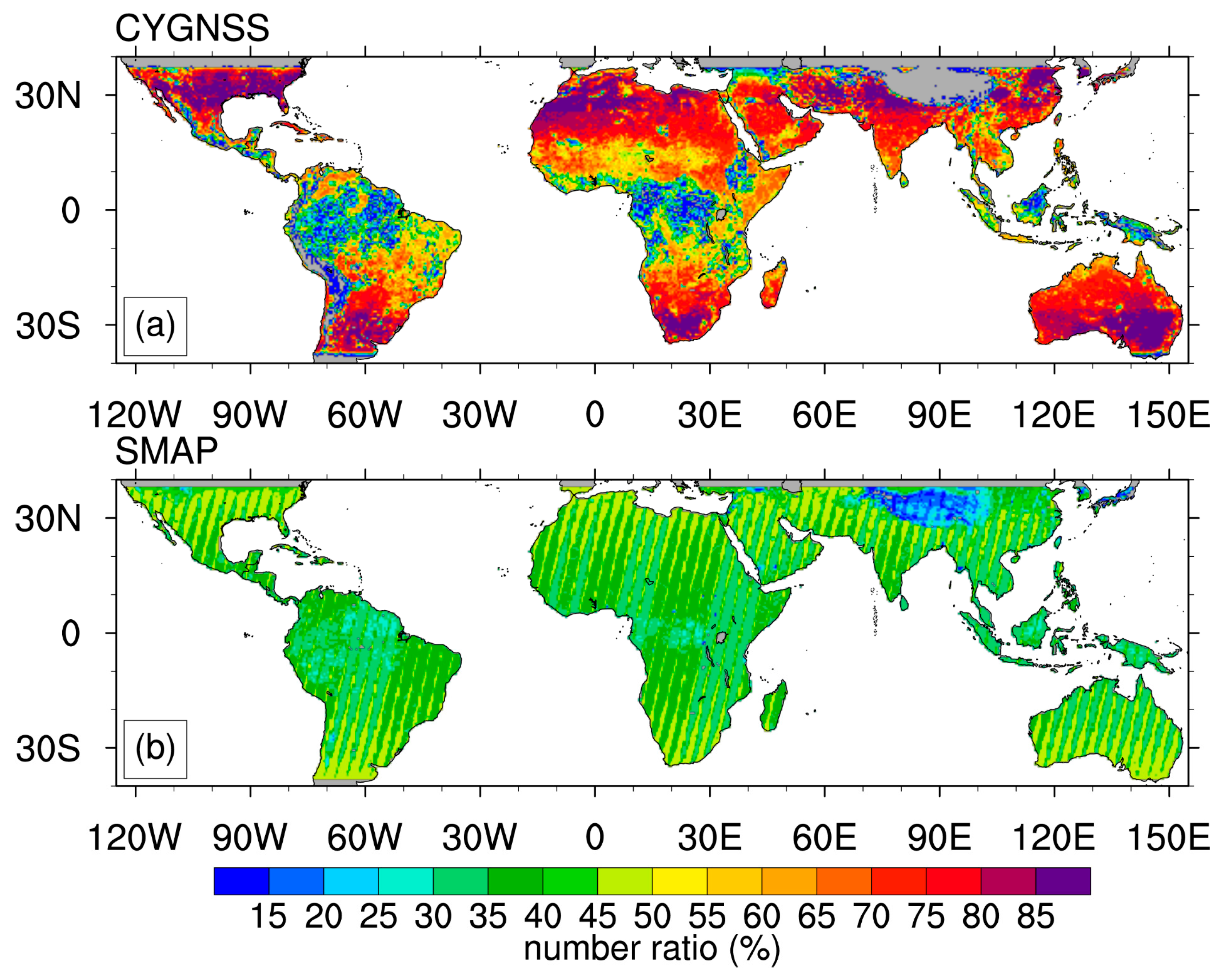
To comprehensively elucidate the spatiotemporal variability of the CYGNSS soil moisture dataset, we undertook a comparative analysis of the CYGNSS data with SMAP, as well as model-derived data from ERA5-land and GLDAS-NOAH, to delineate both similarities and distinctions in soil moisture content. It is pertinent to note that CYGNSS and SMAP, being satellite-retrieved data products, possess certain revisit intervals, leading to the occasional absence of data at specific spatial grids on a daily basis. In contrast, the model-generated data from ERA5-land and GLDAS-NOAH do not have any gaps, ensuring continuous coverage. To provide a clear depiction of data availability, Figure 2 shows the proportion of data volume from the daily CYGNSS and SMAP datasets from 1 January 2018 to 31 December 2022 (encompassing a total of 1825 days, excluding February 29 in leap years).

The CYGNSS dataset exhibits significant variability in temporal coverage across different regions. Near the equatorial belt, specifically in tropical rainforest areas such as the Amazon River Basin, equatorial Africa, and the Indonesian region, the CYGNSS data display a substantial number of missing values. In these regions, only 15% of the time series contain valid data due to the limited ability of satellite retrievals in tropical rainforest and permafrost regions. Additionally, CYGNSS lacks data for the Tibetan Plateau, resulting in extensive missing values attributed to the same limitations. However, in areas excluding these regions, CYGNSS demonstrates a relatively high time coverage rate, exceeding 70%. Particularly noteworthy regions with high coverage include North America, northern Africa, northern India, Pakistan, China, and southern Australia. In contrast, the SMAP data exhibit a lower time coverage rate, approximately 40% on average. Notably, the Tibetan Plateau displays a relatively low time coverage rate, only approximately 20% or less. Seasonal variations have a minimal impact on CYGNSS data, maintaining consistent coverage throughout different seasons. Conversely, during the summer months, SMAP data experience a slight decrease, particularly in regions distant from the equator, resulting in an approximate 5% reduction in data availability.

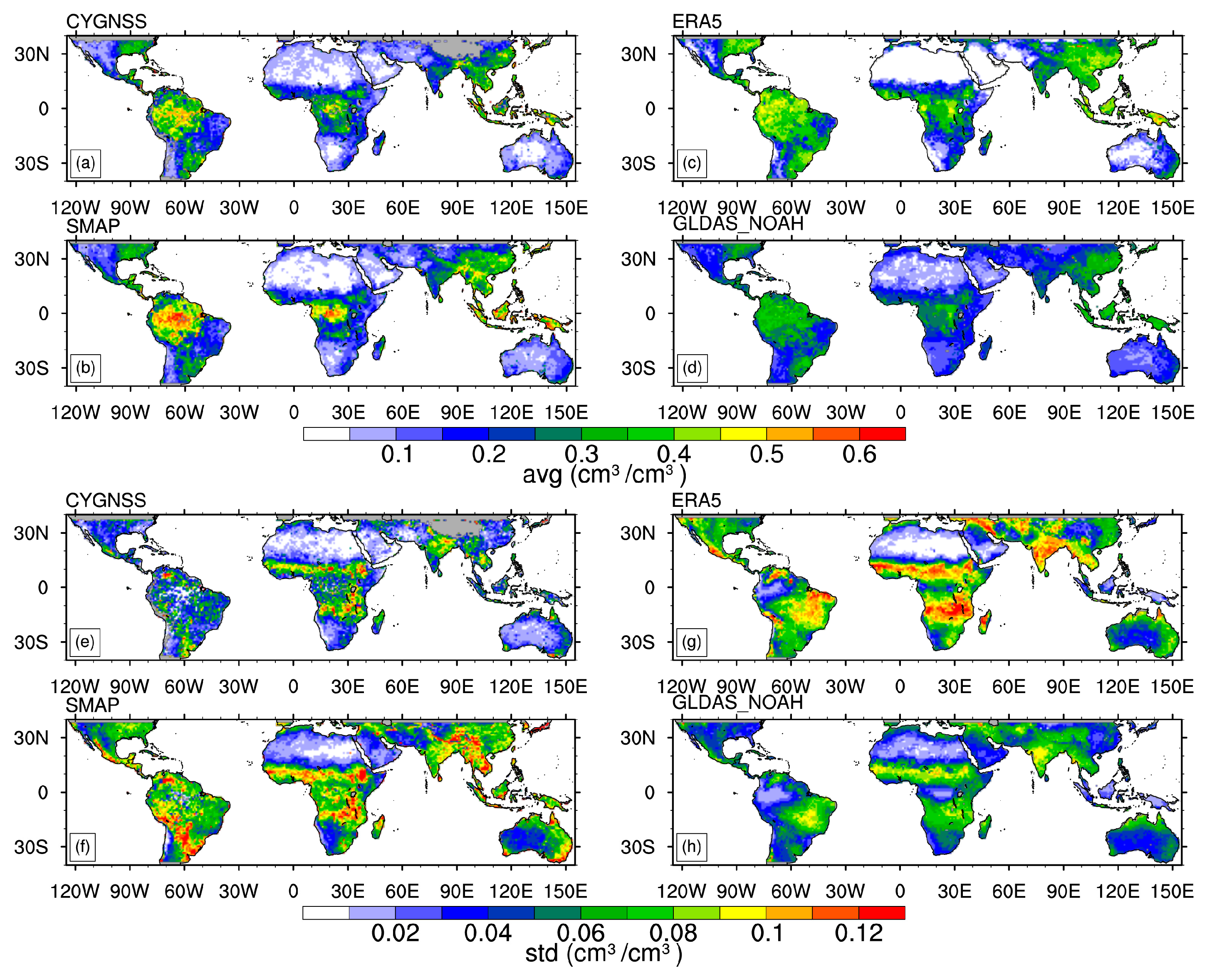
Figure 3 depicts the spatial distribution of the average (Figure 3a–d) and standard deviation (Figure 3e–h) of the four soil moisture datasets. In terms of average soil moisture, all datasets exhibit a consistent spatial structure, with elevated levels observed in the tropical Amazon Basin, Indonesia region, equatorial Africa, southern China, Southeast Asia, and the eastern United States. However, substantial differences in absolute values are notable across the datasets. The CYGNSS values are comparatively smaller than the SMAP data in most regions, particularly in the eastern United States, southern China, Southeast Asia, and eastern Australia, with differences of up to 0.05 cm³/cm³. When compared with the model data (ERA5 and GLDAS-NOAH), the CYGNSS values are smaller in tropical rainforests (such as the Amazon Basin, equatorial Africa, and Indonesia) but larger in other regions, notably, Iran, Pakistan, western India, and northern Australia. Furthermore, the CYGNSS data in tropical rainforest regions are smaller than those of SMAP, yet larger than those of ERA5-land and GLDAS-NOAH.

Figure 3e–h illustrates the standard deviation of the four datasets. Similar spatial patterns are observed, particularly in the Indian region, both sides of the equator in Africa, and eastern Brazil, owing to distinct drought seasons in these areas. Notably, the ERA5 data exhibit a greater standard deviation compared with the other datasets, followed by the SMAP data. CYGNSS demonstrates a larger standard deviation in regions such as the eastern United States, southern Brazil, and the equatorial region of southern Africa while displaying smaller variations in southern China, Indonesia, western North America, the Amazon River Basin, and Australia. The maximum difference in standard deviation between CYGNSS and SMAP reaches 0.05. In comparison with ERA5, CYGNSS exhibits a higher standard deviation in the Sahara region, Arabian region, Iran region, and specific parts of the Amazon River Basin, while generally displaying lower values in other regions. When compared with GLDAS-NOAH, CYGNSS shows a larger standard deviation in the Amazon River Basin, Southeast Asia, the eastern United States, and equatorial Africa, but smaller variations in other regions. In areas where accurate soil moisture estimates are challenging, such as tropical rainforests and desert regions, CYGNSS soil moisture data exhibit smaller standard deviations compared with the SMAP, ERA5, and GLDAS-NOAH results. These variations highlight the complexities and limitations of soil moisture estimation across different geographic and environmental contexts.

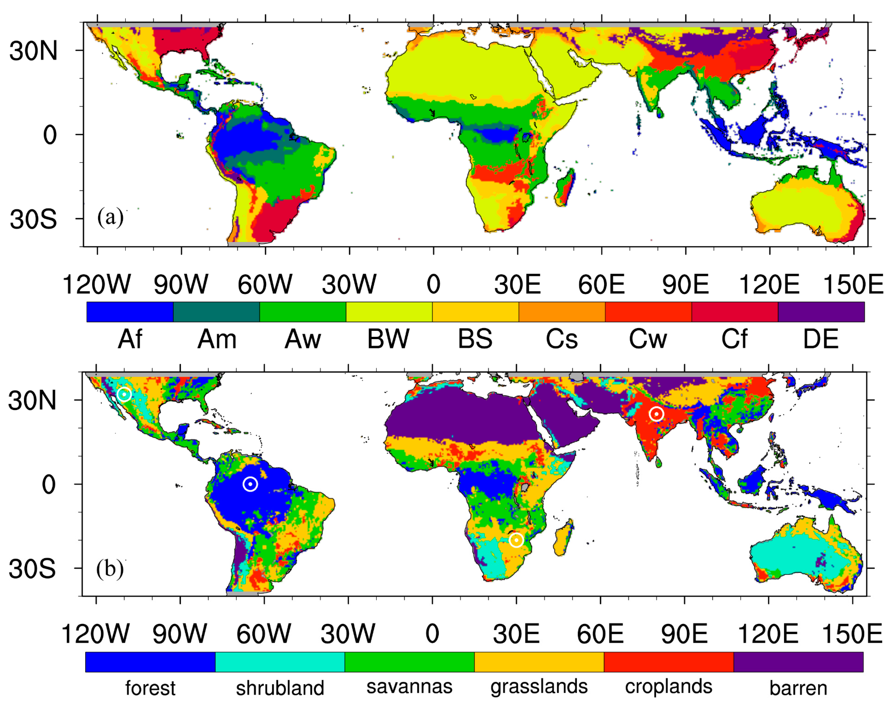
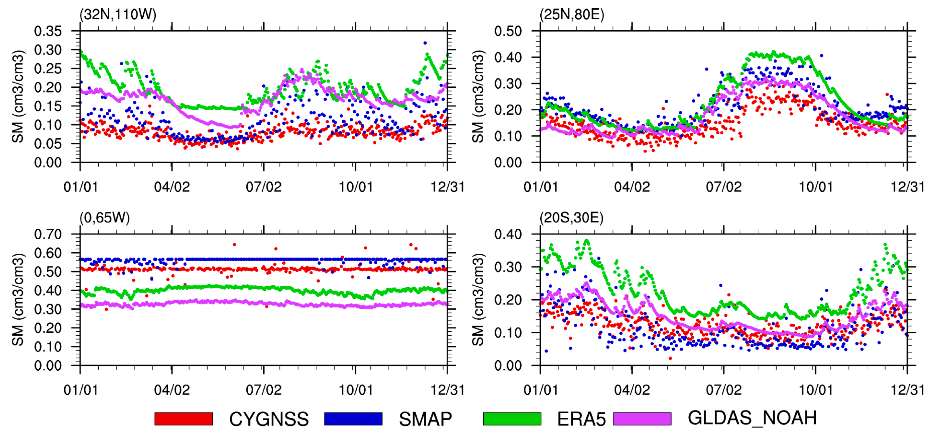
Figure 4 illustrates the temporal dynamics of soil moisture on different days of the year averaged over the period 2018 to 2022 for specific sample points. The first grid point (32°N, 110°W) is in the western United States, characterized by scrubland (land cover type) and an arid, steppe (BS) climate. During summer, autumn, and winter, the soil moisture content is relatively high. Among the datasets, ERA5-land exhibits the highest values, followed by GLDAS-NOAH, while CYGNSS records the lowest average values with minimal variability. The second grid point (25°N, 80°E) is in northern India, featuring croplands (land cover type) and a temperate, dry winter (Cw) climate. Notable distinctions between dry and wet seasons are observed, with all datasets capturing these seasonal variations. The ERA5 data indicate higher average soil moisture values compared with the other datasets, with substantial variability. CYGNSS, in contrast, records the smallest average values and exhibits limited variation. The third grid point (0°, 65°W) is in the Amazon River Basin, characterized by the tropical rainforest (Af) land cover type. While soil moisture variability remains low across all datasets, significant differences emerge in average values. SMAP records the highest, while GLDAS-NOAH reports the lowest, with a disparity of approximately 0.2. The fourth grid point (20°S, 30°E) is in southern Africa, featuring grasslands (land cover type) and a temperate, dry winter (Cw) climate. All datasets display consistent interannual variations. ERA5-land exhibits the highest average values, whereas SMAP shows smaller averages with numerous discrete points, likely due to reduced observation frequency. This analysis provides insights into the spatiotemporal characteristics of soil moisture across diverse geographic locations, highlighting differences between the datasets.

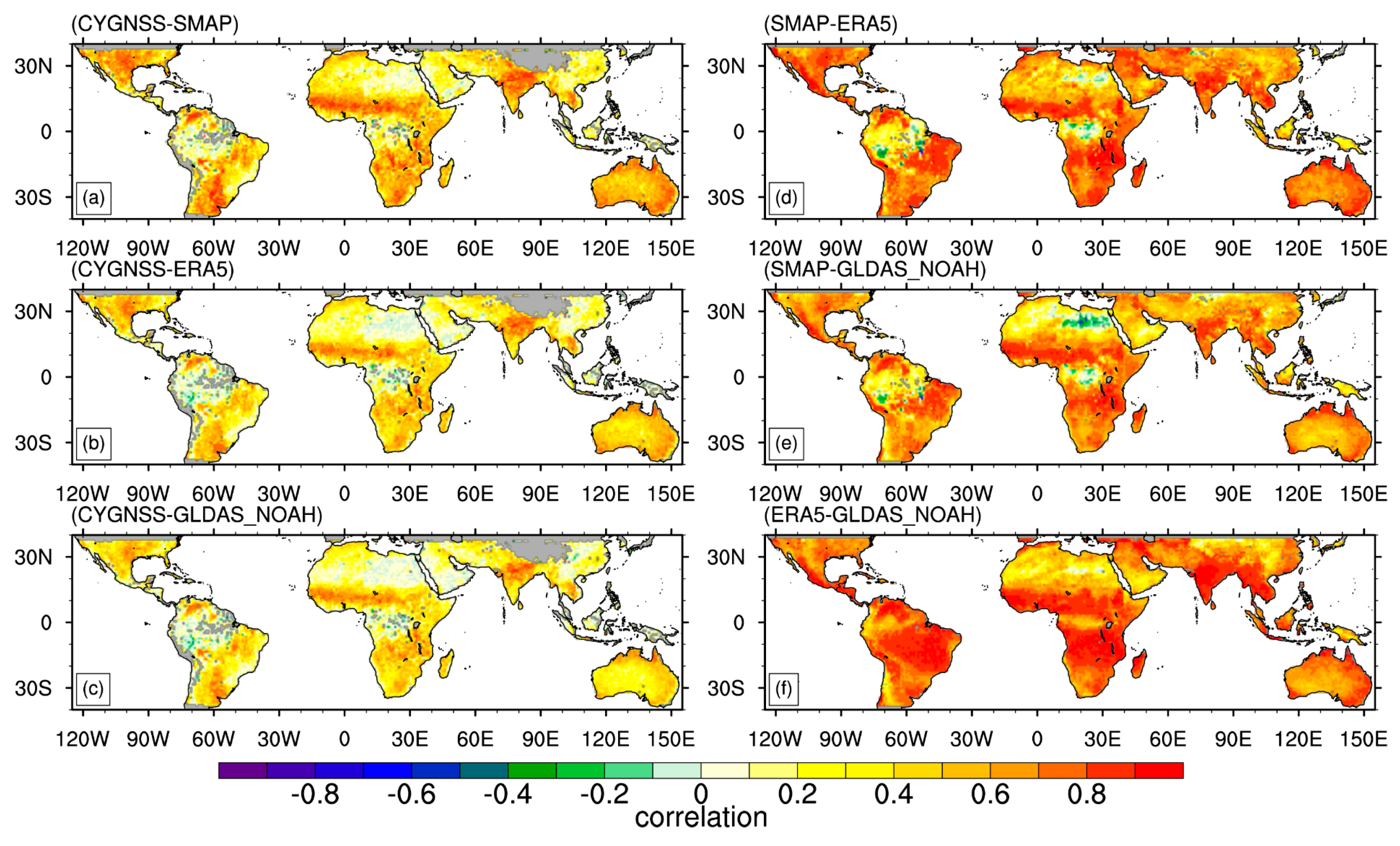
To elucidate the consistency in soil moisture dynamics across the four datasets, we present the pairwise correlation coefficients between CYGNSS, SMAP, ERA5, and GLDAS_NOAH in Figure 5. The results show the concurrence of soil moisture variations among these datasets. Across the studied regions, the correlation coefficients exhibit higher values in areas characterized by significant soil moisture variability, such as North America, India, and equatorial Africa. This phenomenon can be attributed to the presence of robust and distinct signals in these high-variability regions. Notably, the correlation between CYGNSS and SMAP datasets is stronger than the correlation between CYGNSS and the other two datasets. This heightened correlation can be attributed to the incorporation of SMAP data in the CYGNSS soil moisture retrieval process, enhancing the mutual consistency between the two datasets. However, the correlation coefficients between CYGNSS and the remaining three datasets are comparatively smaller when compared with the correlations between the other three datasets, underscoring the nuanced interplay of soil moisture variations captured by these datasets.

The root-mean-square error (RMSE) values of the datasets against each other are depicted in Figure 6, illustrating the disparities among the four soil moisture datasets. Regions with elevated average soil moisture contents, notably, in South America, and near the equatorial regions of Africa, India, southern China, and Southeast Asia, exhibit larger RMSE values. The RMSE between CYGNSS and SMAP is smaller than that between CYGNSS and the other two datasets. The results underscore the strong correlation and interdependency between the CYGNSS and SMAP datasets, highlighting their close connection.

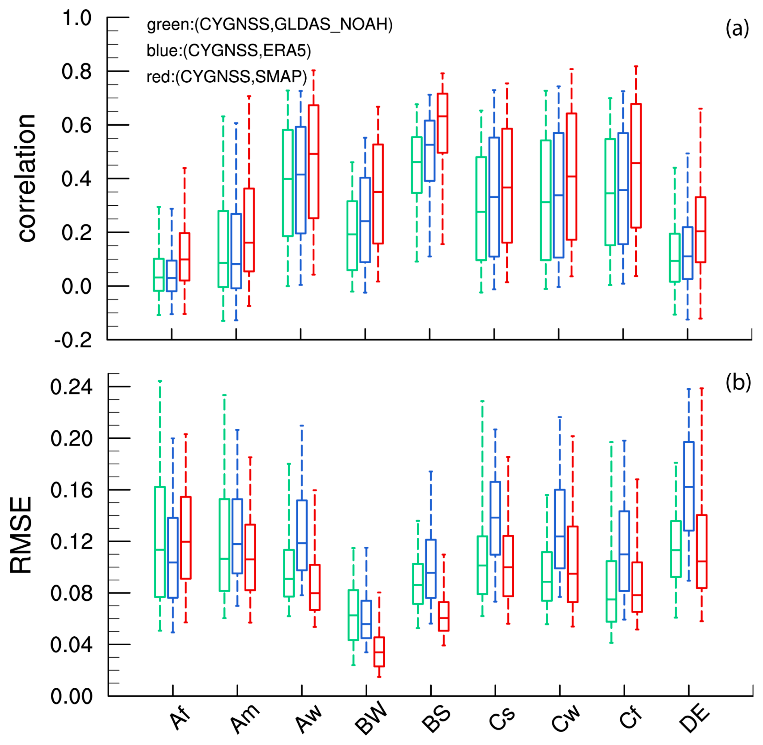
In diverse climate and land cover contexts, the disparities in the average and standard deviation of the soil moisture data from the four datasets are apparent. To scrutinize these distinctions in soil moisture between CYGNSS and the other three datasets, the correlation coefficients and RMSE distributions under distinct climate types are illustrated in Figure 7. The correlation coefficients exhibit notable values in the BS, AW, and CF regions, whereas they are relatively diminutive in the AF, AM, and DE regions. As analyzed earlier, the correlation between CYGNSS and SMAP consistently surpasses that with the other two datasets across varying climate types. Generally, the correlation between CYGNSS and ERA5 outweighs that with GLDAS-NOAH. Regarding RMSE outcomes, discernible disparities emerge in the relationship between CYGNSS and the other three datasets in AF and AM, while more marginal distinctions manifest in BS and BW due to significant divergences in the average soil moisture values in these regions.

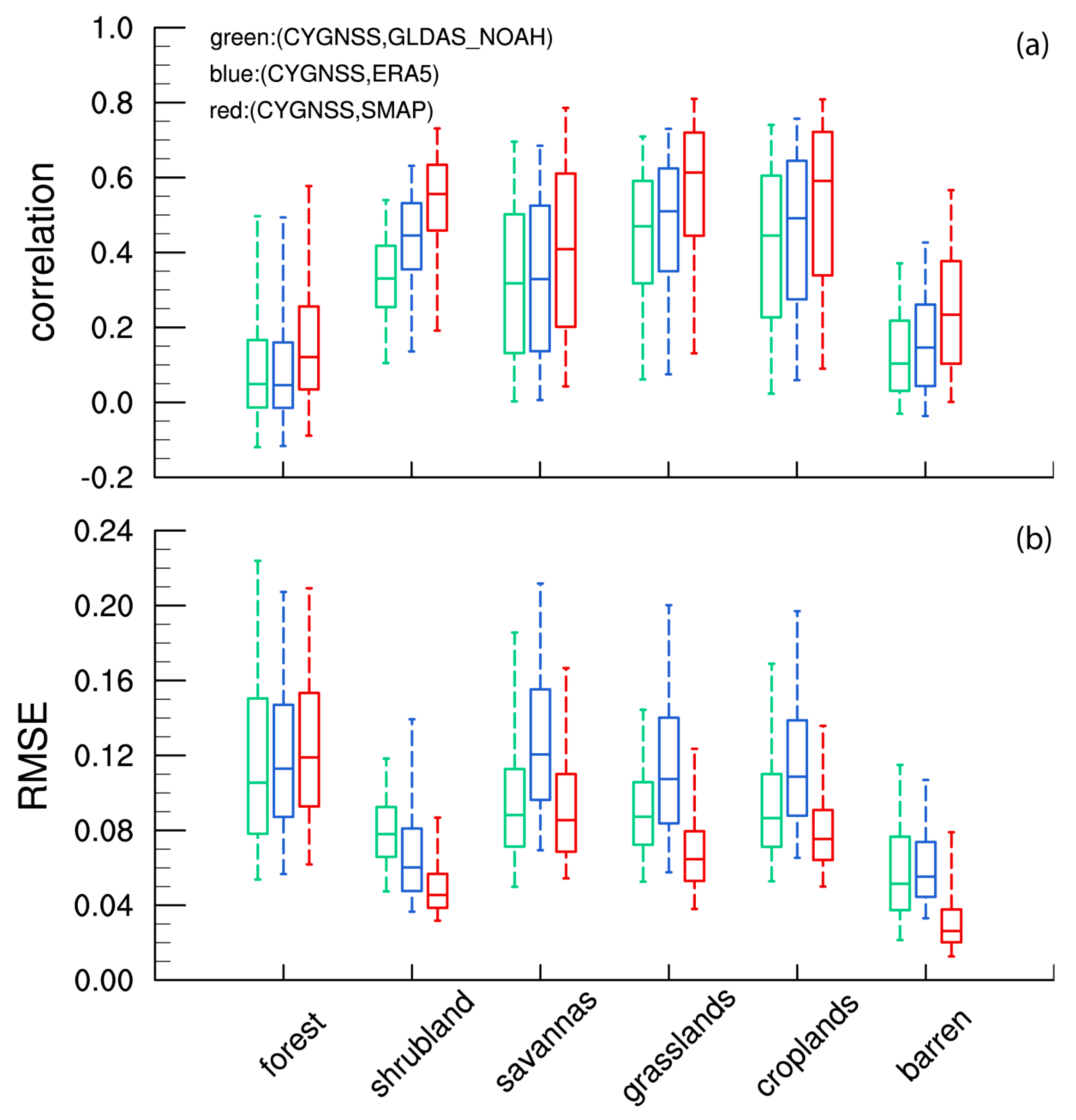
Figure 8 illustrates the correlation coefficients and RMSE values between CYGNSS and the other three datasets under various land cover types. Apparently, the correlation between CYGNSS and SMAP outperforms that between CYGNSS and the other two datasets across diverse land cover types. The CYGNSS-SMAP pair exhibits the smallest RMSE, except for the forest type. The preceding findings indicate that the RMSE values and correlation coefficients between CYGNSS and the other datasets are related to CYGNSS’s own soil moisture average and standard values, respectively.

Table 1. Correlation between CYGNSS soil moisture data and other datasets (SMAP, ERA5, and GLDAS-NOAH) and standard deviation of CYGNSS soil moisture across different climate types and land cover types. Grid numbers are presented in the second row, and correlation coefficients are displayed in the third row.

Af	Am	Aw	BW	BS	Cs	Cw	Cf	DE
3990	3252	12,078	17,920	8209	760	4355	4152	1015
0.28	0.45	0.59	0.76	0.31	0.29	0.69	0.54	0.27
Forest	Shrubland	Savanna	Grassland	Cropland	Barren
8993	6416	11,333	11,648	5416	11,849
0.45	0.37	0.61	0.44	0.65	0.69

provides the correlation coefficients between the average correlation of CYGNSS with the other three datasets and the standard deviation of CYGNSS soil moisture data for different land cover and climate types. The correlation coefficients between the RMSE and average soil moisture values are presented in

Table 2. Correlation between root-mean-square error (RMSE) of CYGNSS soil moisture compared with other datasets (SMAP, ERA5, and GLDAS-NOAH) and average soil moisture of CYGNSS across different climate types and land covers. Grid numbers are presented in the second row, and correlation coefficients are displayed in the third row.

Af	Am	Aw	BW	BS	Cs	Cw	Cf	DE
3990	3252	12,078	17,920	8209	760	4355	4152	1015
0.19	0.24	0.51	0.77	0.48	0.52	0.48	0.15	0.54
Forest	Shrubland	Savanna	Grassland	Cropland	Barren
8993	6416	11333	11648	5416	11,849
0.16	0.67	0.34	0.53	0.35	0.91

, along with corresponding grid points for distinct land cover and climate types. The correlation and standard deviation consistently show a significantly positive relationship across all climate and land cover types, particularly in the BW and Cw climate types, with the correlation coefficient exceeding 0.65. Correlation coefficients above 0.6 were achieved in barren, savanna, and grassland. Regarding the RMSE and average soil moisture values, notable correlations were observed, specifically reaching 0.77 in BW, 0.67 in shrubland, and 0.91 in barren. These results indicate the intricate relationship between RMSE, average values, correlation coefficients, and standard deviation. However, the variations in this relationship across different climates and land cover types emphasize the need to carefully consider the soil moisture accuracy obtained from CYGNSS data under specific climate conditions.

5. Performance Evaluation of Drought Indicators

Following the description in the methodology section, we employed soil moisture data derived from CYGNSS, SMAP, ERA5-land, and GLDAS-NOAH to formulate drought indicators. The computation of drought indicators was based on daily soil moisture values, which were subsequently averaged to yield monthly results. Since CYGNSS and SMAP are satellite products, they do not provide data on a daily basis. Upon monthly aggregation, we found that for the majority of grid points, both satellite datasets offer 60 months of data coverage spanning from January 2018 to December 2022 (figure not shown). Meanwhile, CYGNSS exhibits missing values for grid points within the Amazon River Basin and equatorial Africa. The Tibetan Plateau lacks CYGNSS data entirely, whereas SMAP data do exist in this region, albeit with significant periods of missing values. Consequently, our analysis did not include the drought situation on the Tibetan Plateau.

5.1. Drought Characteristics

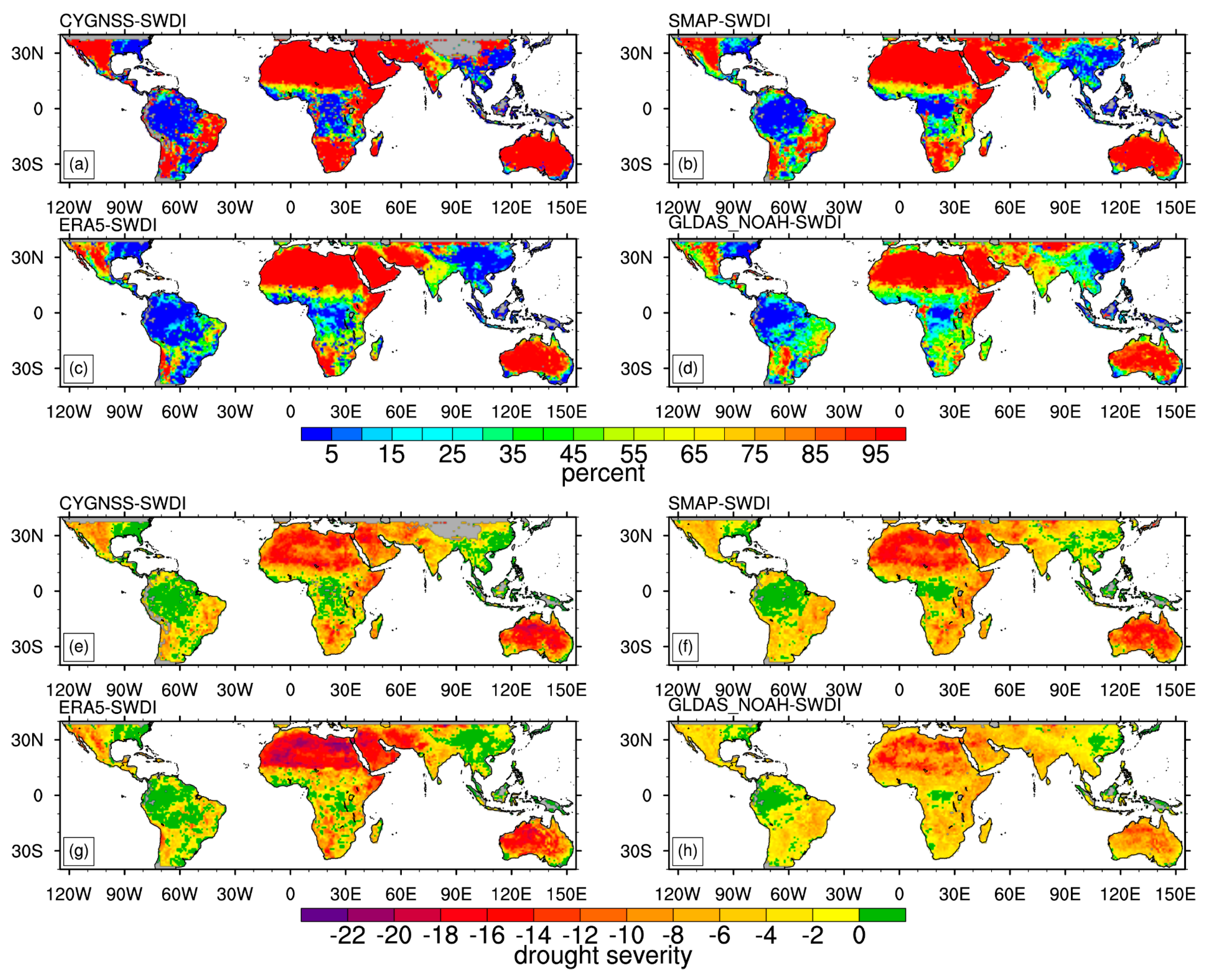
In this section, we evaluate the drought indices derived from different soil moisture datasets based on drought percentage and intensity, aiming to discern their effectiveness in depicting drought conditions. Figure 9 illustrates the drought characteristics represented by the SWDI across the four datasets. Concerning the drought percentage (Figure 9a–d), all datasets indicate prolonged water scarcity in desert areas, grasslands, and specific regions such as the Sahara Desert, Arabian Desert, South African grasslands, and parts of Australia. These areas consistently exhibit extended periods of an insufficient water supply for plant needs, signifying persistent drought conditions.

Specifically, the CYGNSS data display a broader range and more intense long-term drought conditions (with percentages exceeding 95%) in comparison with the other datasets. Conversely, regions with low drought occurrence (< 5%) are identified in the Amazon River Basin, equatorial Africa, eastern North America, southern China, and Southeast Asia. CYGNSS, when contrasted with SMAP and GLDAS-NOAH, portrays a larger extent of low-percentage drought conditions, primarily due to higher soil moisture values detected near the equatorial regions of Africa and South America. Additionally, the drought percentage derived from CYGNSS surpasses that from other datasets in western North America.

Figure 9e–h presents the drought intensity from January 2018 to December 2022, where green (values greater than 0) indicates the absence of severe drought events. The SWDI from all four datasets exhibits similar spatial patterns and numerical values regarding drought intensity. The intensity is notably higher in the Sahara Desert and Arabian regions, while relatively milder drought conditions prevail in southern China, eastern North America, and the Amazon River Basin. In some areas, particularly in southern China and parts of eastern North America and the Amazon River Basin, no drought events have been identified. Comparatively, CYGNSS identifies more regions without significant drought, distinguishing it from the other datasets.

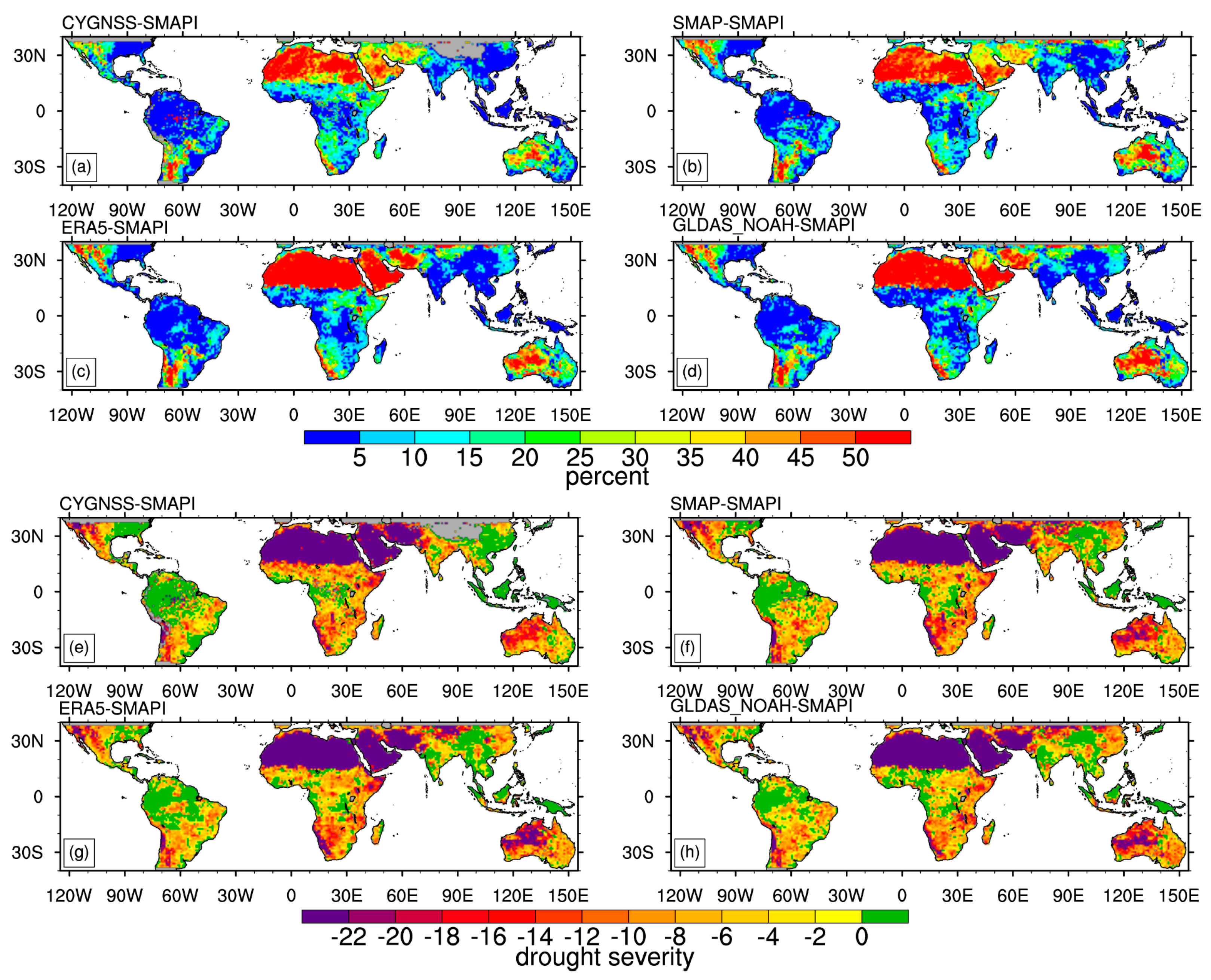
In contrast with the SWDI, the SMAPI is used to calculate the drought percentage and severity, they are the drought indicators from soil moisture anomalies, enabling a comparison of values across various grid points. Figure 10 shows the spatial distribution of the drought percentage (a–d) and drought severity (e–h) derived from the SMAPI based on the four datasets. Overall, there is a striking similarity in both the drought percentage and severity characteristics among the four datasets. This uniformity arises from the Cumulative Distribution Function (CDF) correction applied to the soil moisture data from CYGNSS, SMAP, and GLDAS-NOAH, with reference to the ERA5 dataset, ensuring consistency in their statistical distributions, including means and standard deviation. These results depict drought characteristics with a high degree of similarity. Nonetheless, some distinctions persist when comparing CYGNSS with the other three datasets. For instance, the drought percentages calculated with CYGNSS are lower than those derived from the other three datasets in regions such as western North America, southern China, and western Australia. In terms of drought severity, CYGNSS consistently reports lower values than the other datasets, particularly in southern China and western Australia. These differences emphasize the subtle disparities in drought characteristics between CYGNSS and the other datasets.

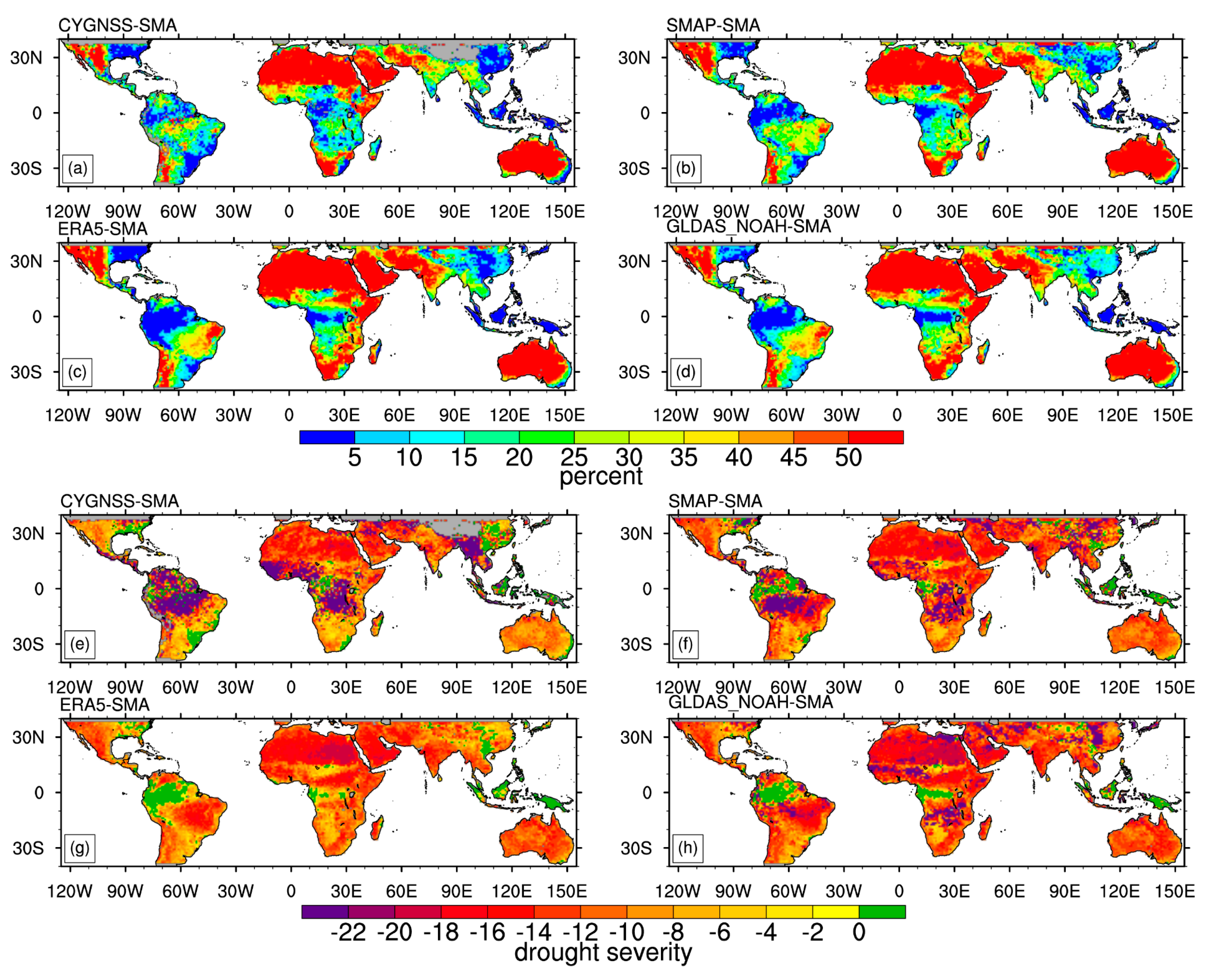
The drought characteristics derived from the Soil Moisture Anomaly (SMA) exhibit remarkable similarities across the four datasets, as illustrated in Figure 11. When compared with the SMAPI, the SMA indicates higher drought percentages in regions such as South America, equatorial Africa, India, Southeast Asia, and southern China. This discrepancy can be attributed to the differing criteria employed by these two indices to identify severe drought conditions. Meanwhile, the SMA calculated from CYGNSS demonstrates lower drought percentages and reduced drought severity in southern China and eastern Brazil compared with the results derived from the other three datasets. It is crucial to acknowledge a noteworthy observation: the outcomes derived from satellite-based soil moisture assessments, encompassing both the CYGNSS and SMAP datasets, tend to overstate both the proportion and intensity of drought in the Amazon River Basin. This discrepancy may stem from the inherent limitations of satellite observation accuracy in tropical forest regions, highlighting the complexities involved in accurately capturing drought dynamics in such ecologically sensitive areas.

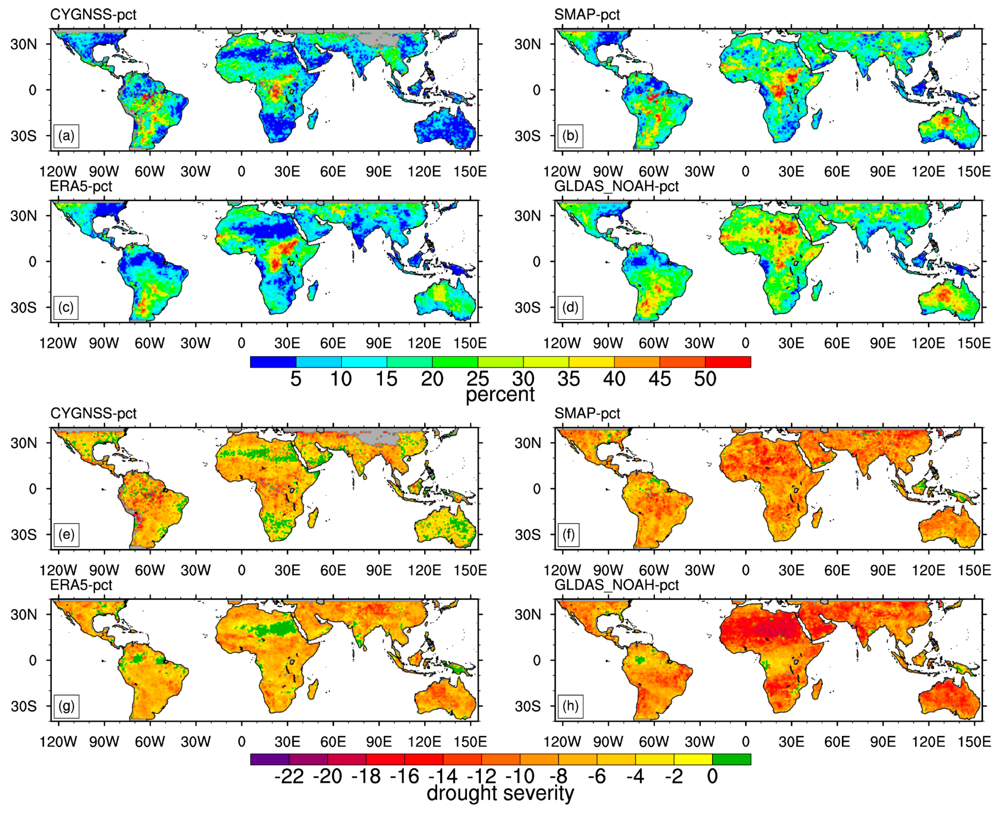
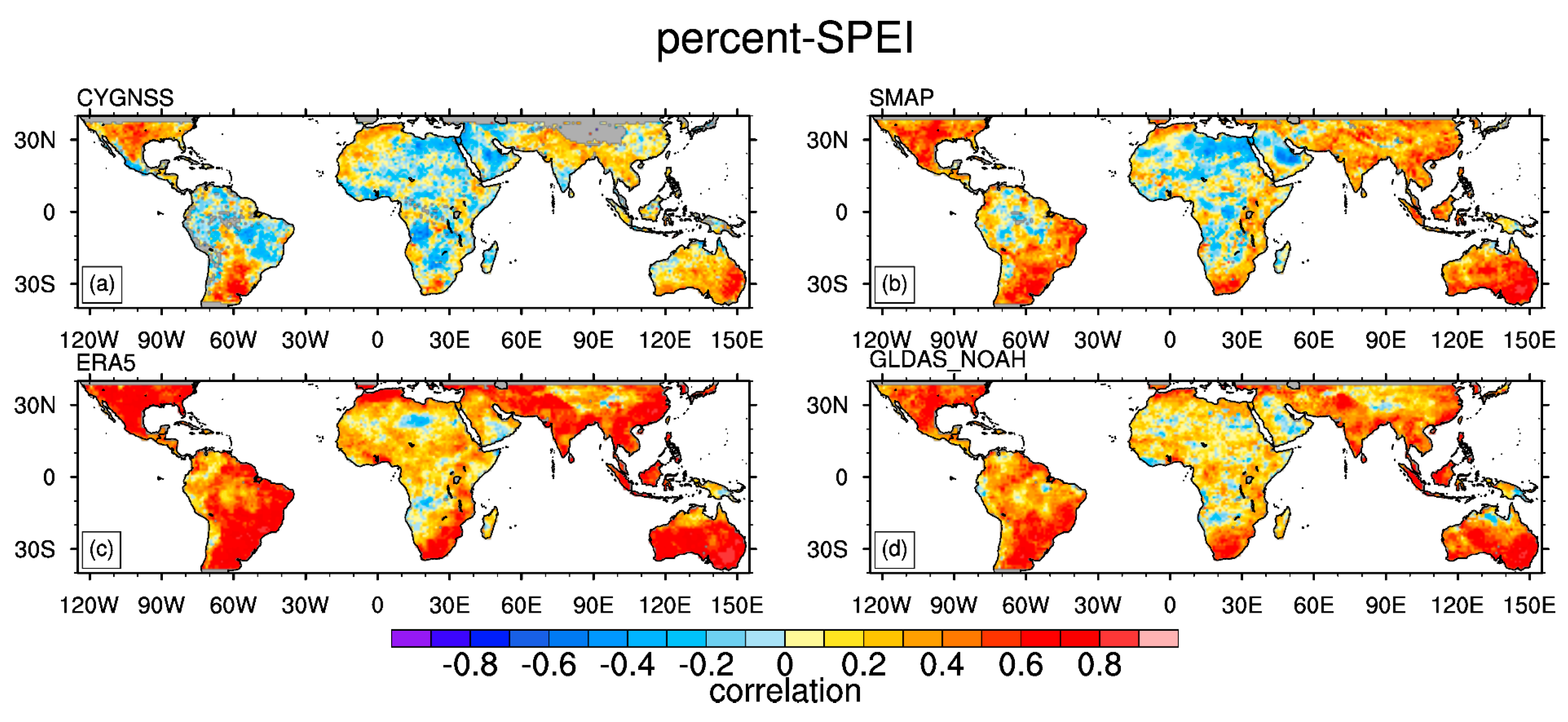
Figure 12 illustrates the drought percentage and severity based on the soil moisture percentiles computed from the four datasets. The drought percentage and severity derived from CYGNSS and ERA5 appear to be comparatively lower than those obtained from SMAP and GLDAS-NOAH. This trend is particularly pronounced in regions such as North America, India, and Australia, where CYGNSS and ERA5 consistently indicate reduced drought percentages and severity when compared with SMAP and GLDAS-NOAH. Building upon the earlier findings, it is worth emphasizing that the drought percentage and severity values derived from CYGNSS remain notably lower in specific regions, such as Australia and southern China, in contrast with the corresponding outcomes from the other three datasets.

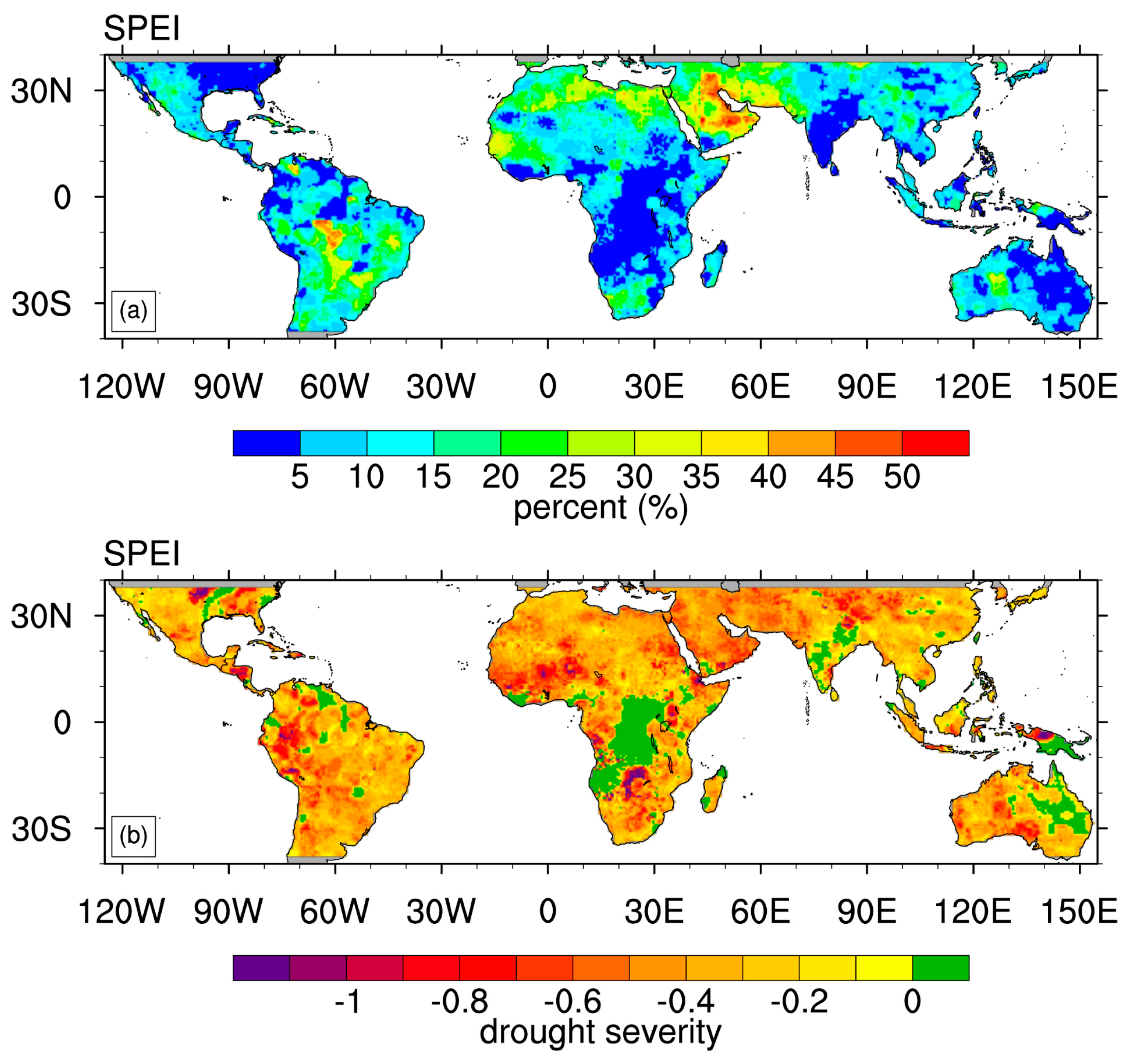
For reference purposes, the drought characteristics defined by the Standardized Precipitation Evapotranspiration Index (SPEI) are presented in Figure 13, with the selected drought scenario being defined as cases where the SPEI value is less than −1.5. The results derived from the SPEI analysis indicate that regions experiencing extreme drought are predominantly concentrated in specific areas, including South America (specifically Brazil and Argentina), the Sahara Desert, and the Arabian Desert, collectively accounting for approximately 25% of the studied regions. Contrastingly, regions such as India, equatorial Africa, eastern North America, and eastern Australia exhibit relatively small drought percentages, with some areas exhibiting lower than 5%. Furthermore, examining drought intensity reveals that equatorial Africa, eastern Australia, and India experience comparatively minor instances of drought, with some regions even reporting no occurrence of drought. These findings underscore the variability in drought conditions across different geographic regions from different drought indicators based on different soil moisture datasets.

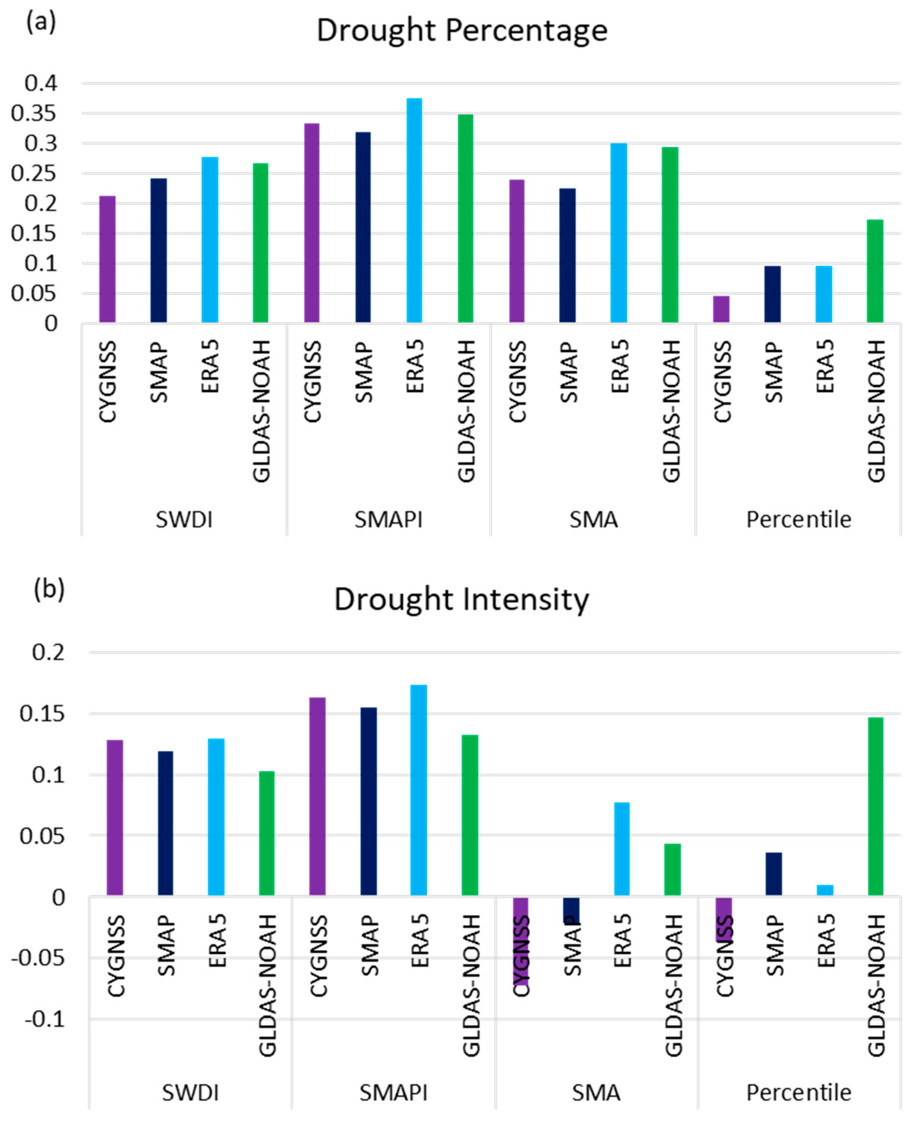
When comparing the drought characteristics derived from the SPEI with those based on soil moisture, notable disparities emerge in terms of drought percentage values, their spatial distributions, and the spatial structure of drought intensity. To quantify and assess these differences across various soil-moisture-based drought indicators, we computed the spatial correlations of the drought percentage and drought intensity between the SPEI and the results obtained from different soil moisture datasets. These correlations are presented in Figure 14. Concerning the drought percentage, the spatial correlations between the SPEI and the different soil-moisture-based drought indicators, namely, the SWDI, SMAPI, and SMA, are generally strong, all exceeding 0.2, with the exception of the Percentile-based indicator. Among the three drought indicators (the SWDI, SMAPI, and SMA), the results obtained from ERA5 show the highest correlation with the SPEI, outperforming other soil moisture datasets. Furthermore, the spatial correlation between CYGNSS and SPEI is superior to that of SMAP. Conversely, for drought intensity, the spatial correlations between SPEI and the different drought indicators derived from various soil moisture datasets are generally weak. The performance of the SMA indicator is notably poor, with negative correlations observed in the cases of the CYGNSS and SMAP results. While the correlations for the SWDI and SMAPI based on different soil moisture datasets exceed 0.1, the results from CYGNSS rank second only to those obtained from ERA5. These findings highlight the ability of CYGNSS to depict drought conditions using certain drought indicators.

5.2. Comparison with SPEI

The findings in the previous section elucidate the distinctions in drought characteristics delineated by various drought indices utilizing diverse soil moisture datasets, which also differ from the outcomes derived from the SPEI. To further evaluate the efficacy of soil-moisture-based drought indices, we computed their correlation coefficients with the SPEI time series. We analyzed several metrics, including the TS, hit rate, false alarm rate, and miss rate for drought events.

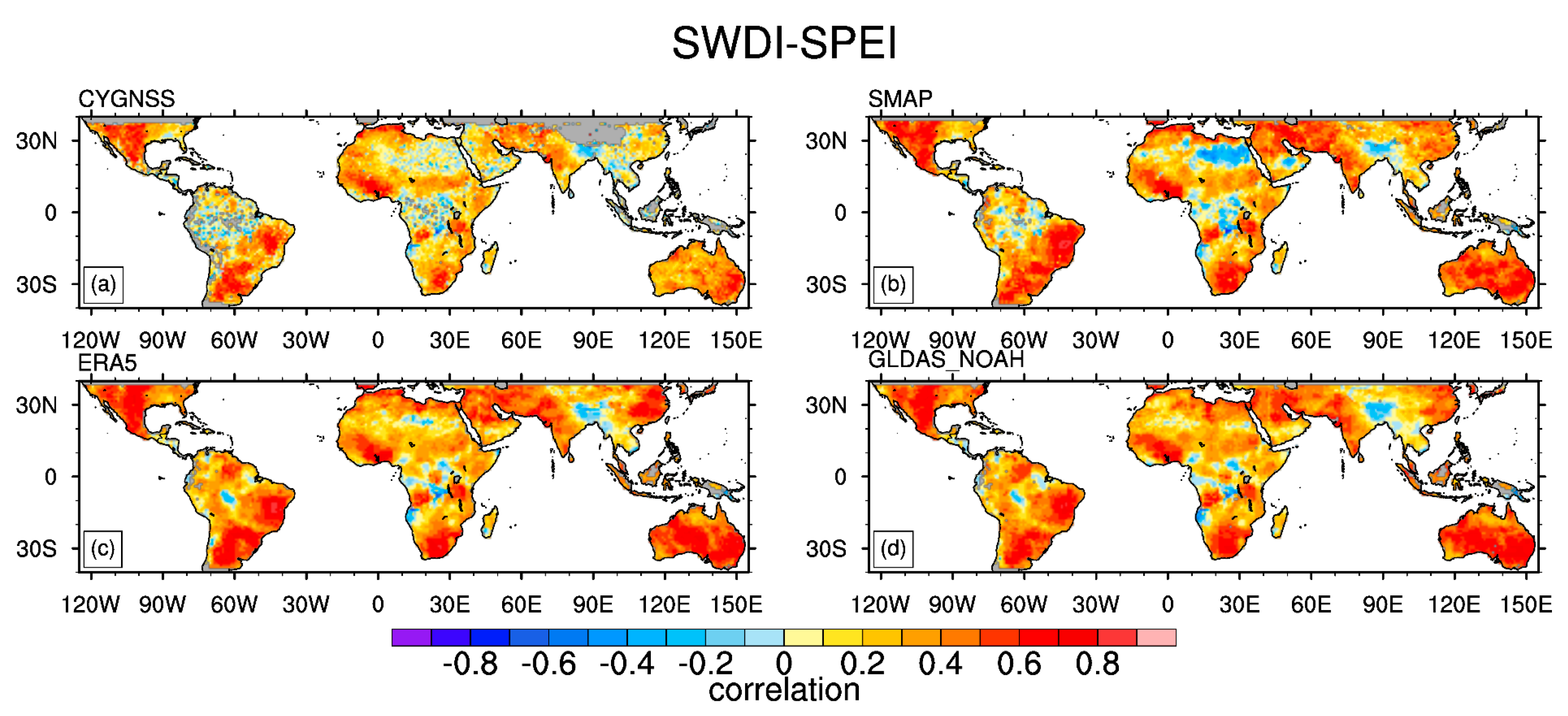
Figure 15 illustrates the correlation between the SWDI derived from the four datasets and the SPEI. The results reveal a similar correlation pattern across these four datasets, with higher values in western North America, southern South America, South Africa, and Australia. Among the datasets, ERA5 demonstrates the strongest correlation with the SPEI. Nevertheless, CYGNSS exhibits comparatively lower correlation coefficients, especially in regions such as southern China, India, and Pakistan. Considering the spatial grid proportion where correlation coefficients exceed 0.23 (critical value at the 90% confidence level with 50 degrees of freedom), CYGNSS accounts for only 48.2%, while SMAP achieves 64.7%. In contrast, ERA5 (and GLDAS-NOAH) outperforms the others, reaching an impressive proportion of 73.0% (72.3%).

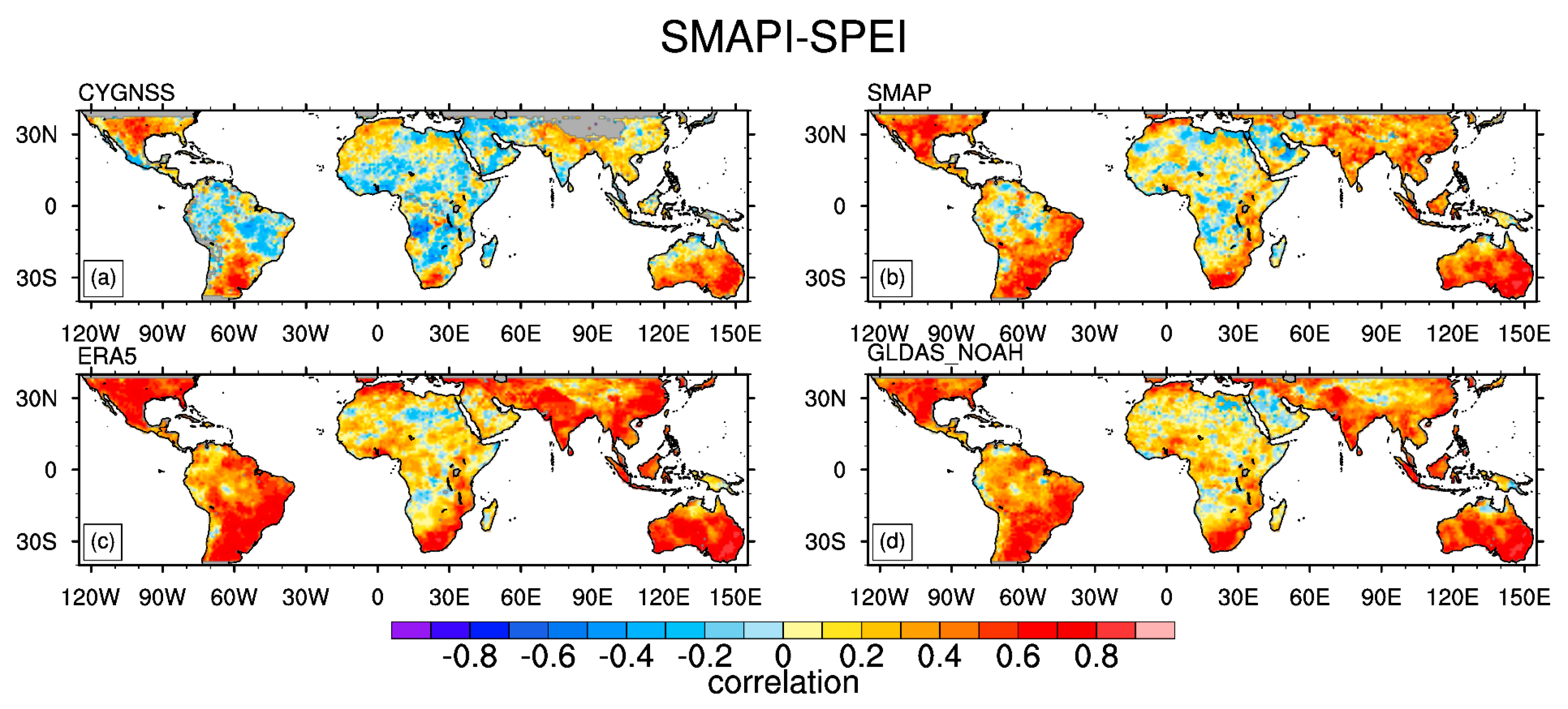
The correlation between the SMAPI and SPEI is presented in Figure 16. It shows that the correlation coefficients for CYGNSS exhibit a significant decline when compared with the SWDI condition. This decline is particularly pronounced in Africa, where several regions display negative correlation coefficients. CYGNSS consistently yields results with the lowest correlation coefficients in comparison with the other three datasets. The results corresponding to ERA5 rank the highest, followed by GLDAS-NOAH, aligning with the trends observed in the SWDI results. 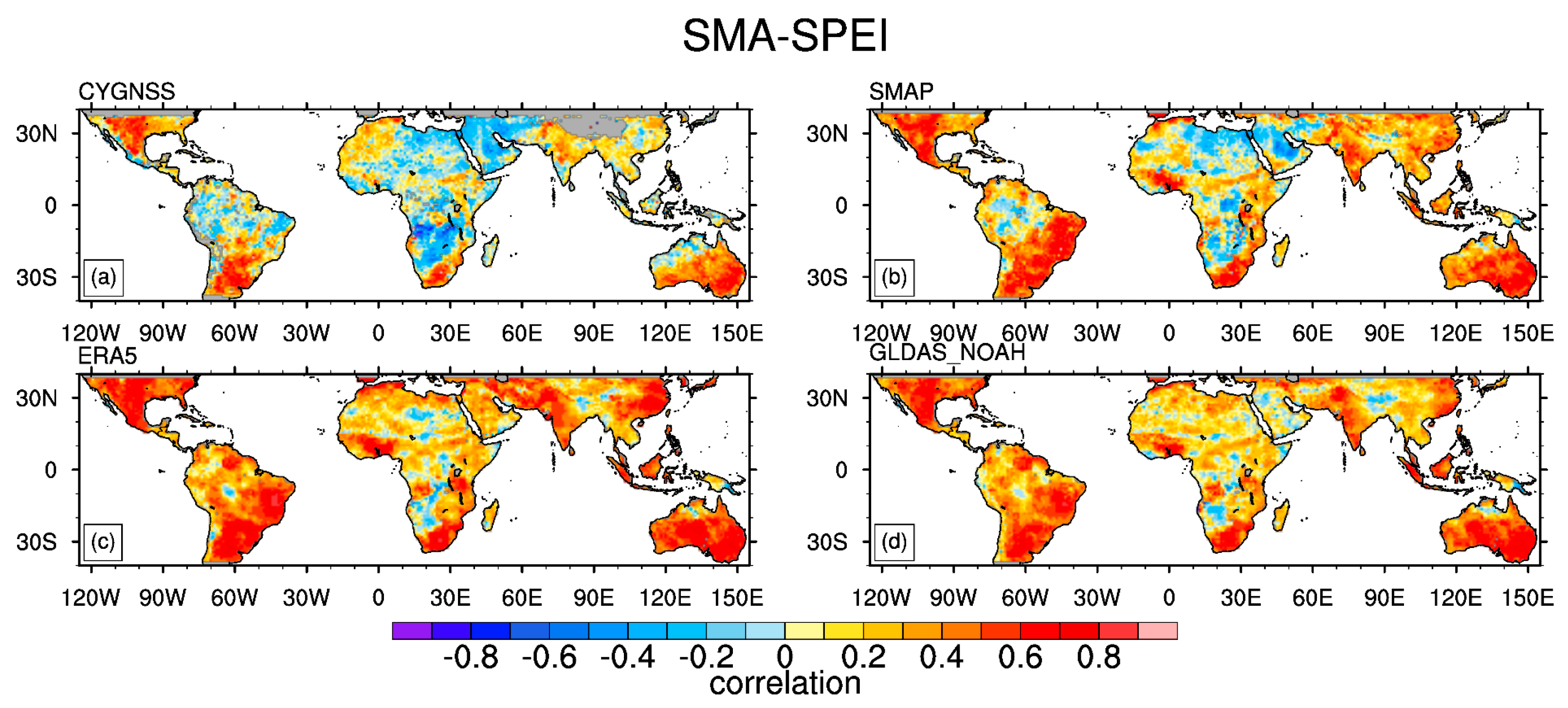Figure 17 and Figure 18, depicting the SMA and Percentile, respectively, exhibit similar patterns to the SMAPI. In accordance with these drought indices, ERA5 consistently holds the highest proportion of spatial grids, with correlation coefficients surpassing the critical value of 0.23. In contrast, CYGNSS consistently ranks the lowest, indicating that CYGNSS can characterize drought situations to some extent, although its performance does not consistently match that of the other three datasets.

Utilizing the SPEI results as a benchmark, different drought indicators derived from various soil moisture datasets for severe drought events from January 2018 to December 2022 are evaluated. Figure 19 illustrates the outcomes obtained from the SWDI. The TSs depicted in Figure 19 reveal that in comparison with drought events identified with the SPEI, the SWDI exhibits relatively low scores overall. The maximum value, approximately 0.3, is observed in northern Africa, the Arabian region, and Iran. In contrast, in several regions including eastern North America, southern China, India, the Amazon Basin, Africa, and eastern Australia, the TSs are notably low, hovering at around 0.02 or even lower. The poor TSs stem from an excessive identification of drought events based on the SWDI assessments in most regions (except for southern China, Southeast Asia, the Amazon River Basin, and eastern North America). This abundance of identified drought events results in high hit rates, often reaching 0.9 in most regions. Consequently, the miss rates remain low, but the false alarm rates are elevated, surpassing 0.9, leading to diminished TSs. Meanwhile, in southern China, Southeast Asia, the Amazon River Basin, and eastern North America, the SWDI fails to accurately identify sufficient drought events. As a result, these regions exhibit high miss rates exceeding 0.9 and low hit rates, culminating in diminished TSs. When compared with the other three datasets, CYGNSS exhibits spatial structures and TSs that are quite similar. However, in certain regions such as western North America, CYGNSS yields smaller scores compared with the other three datasets.

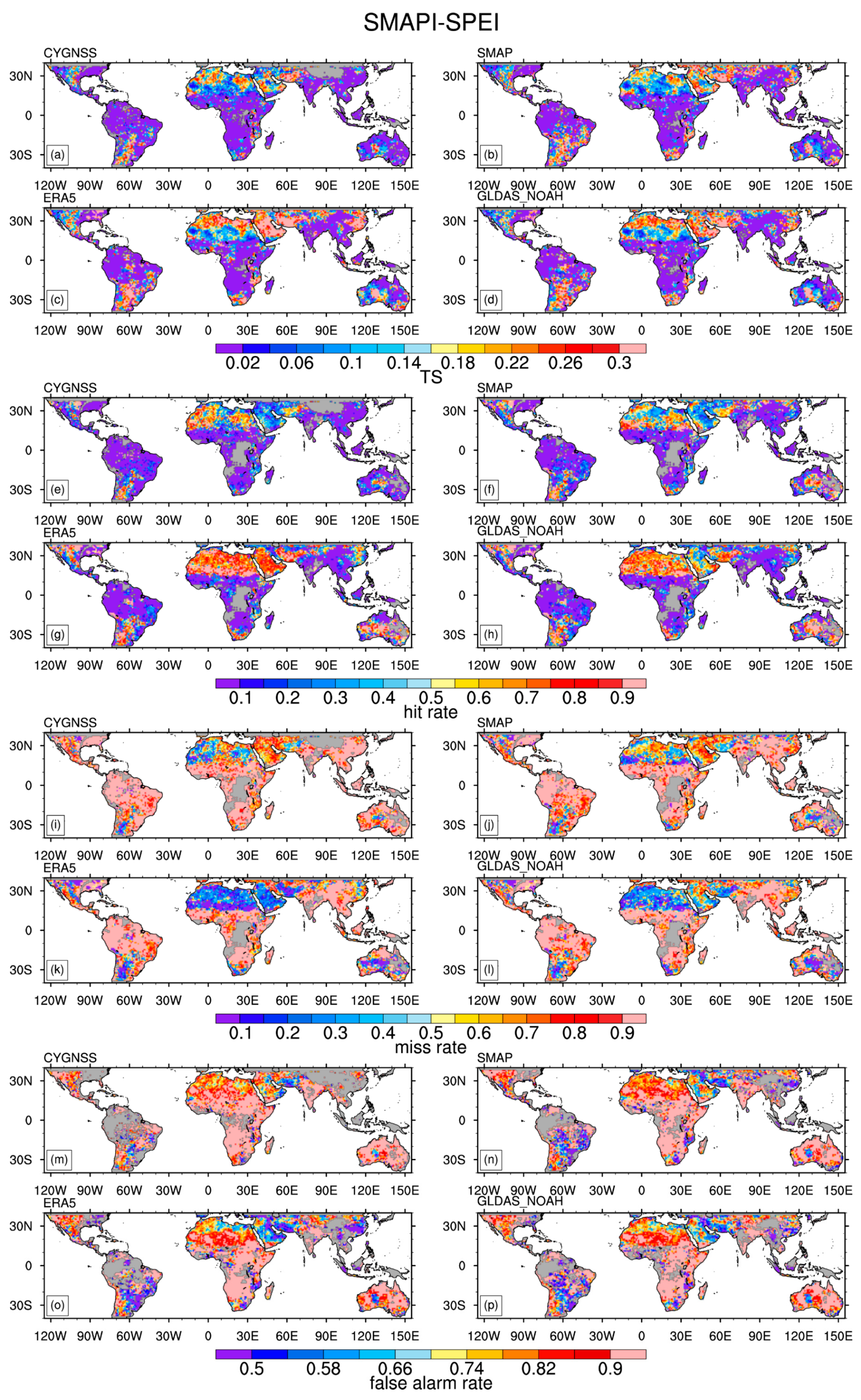
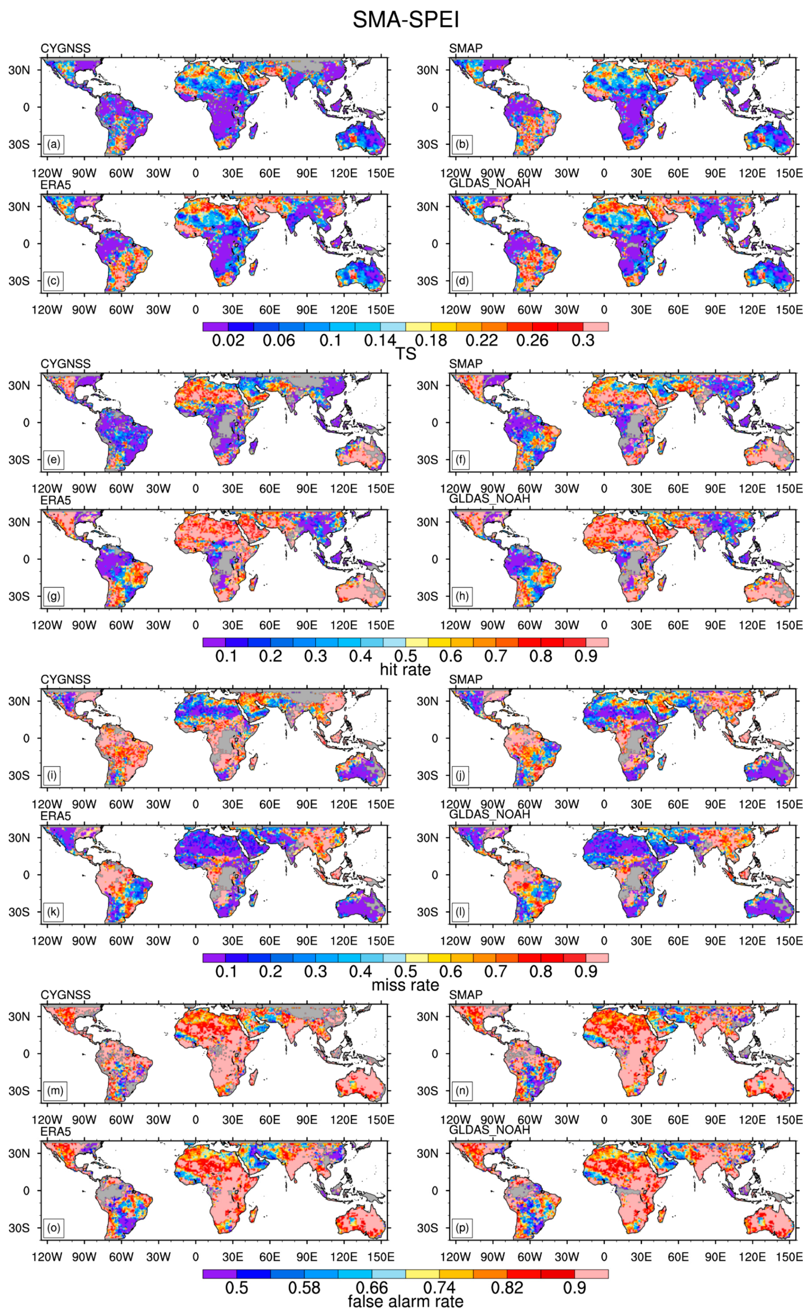
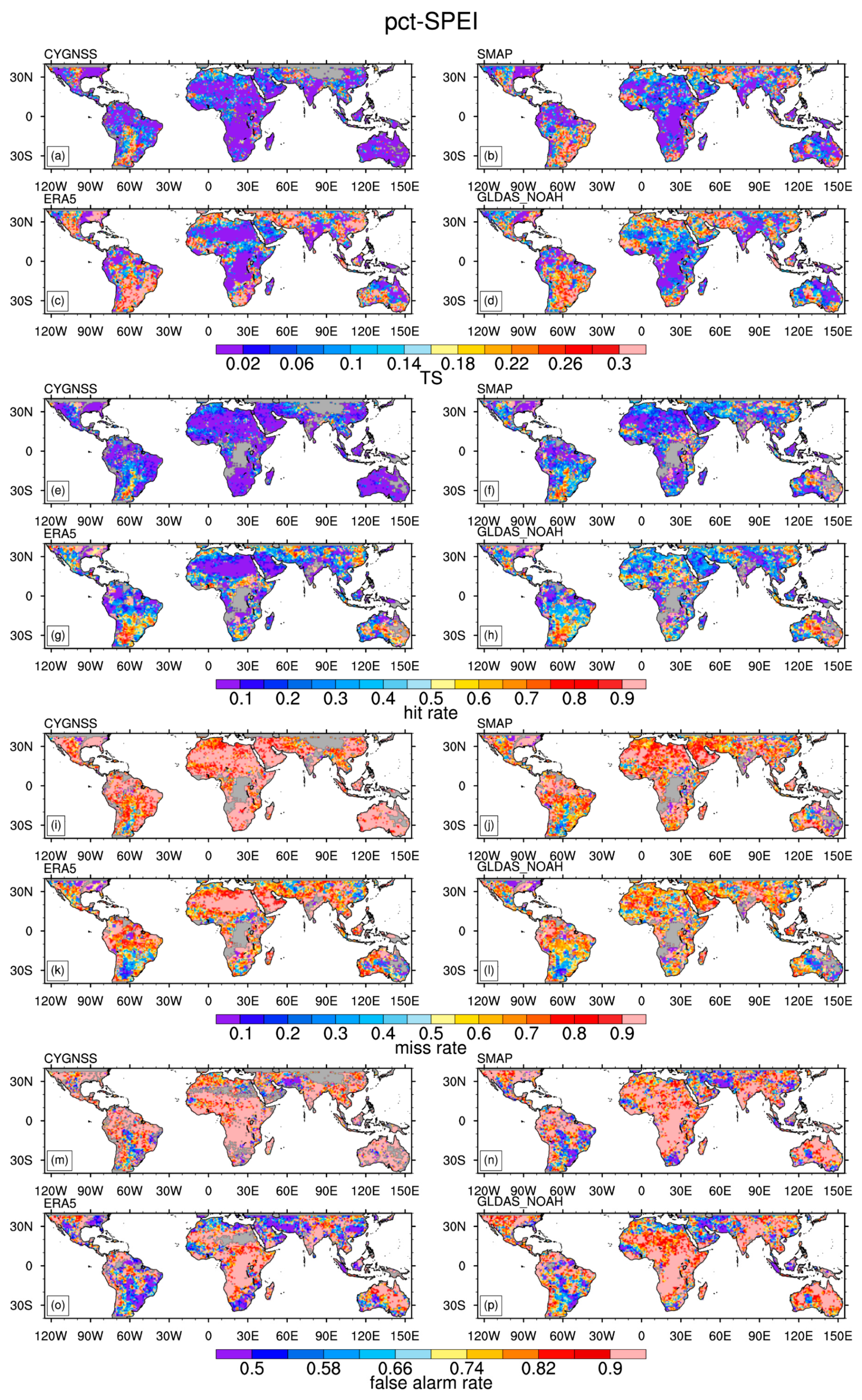
The skill scores for the SMAPI, SMA, and Percentile are presented in Figure 20, Figure 21 and Figure 22, respectively. The spatial patterns of TSs for these indices closely resemble those obtained from the SWDI. Nevertheless, Percentile exhibits a poorer performance compared with the other three drought indicators (the SWDI, SMAPI, and SMA), with high miss rates and false alarm rates. Meanwhile, the TSs from CYGNSS show similar patterns and values to those from the other three soil moisture datasets, although the TS from CYGNSS in southern China consistently lags behind that of the other three datasets.

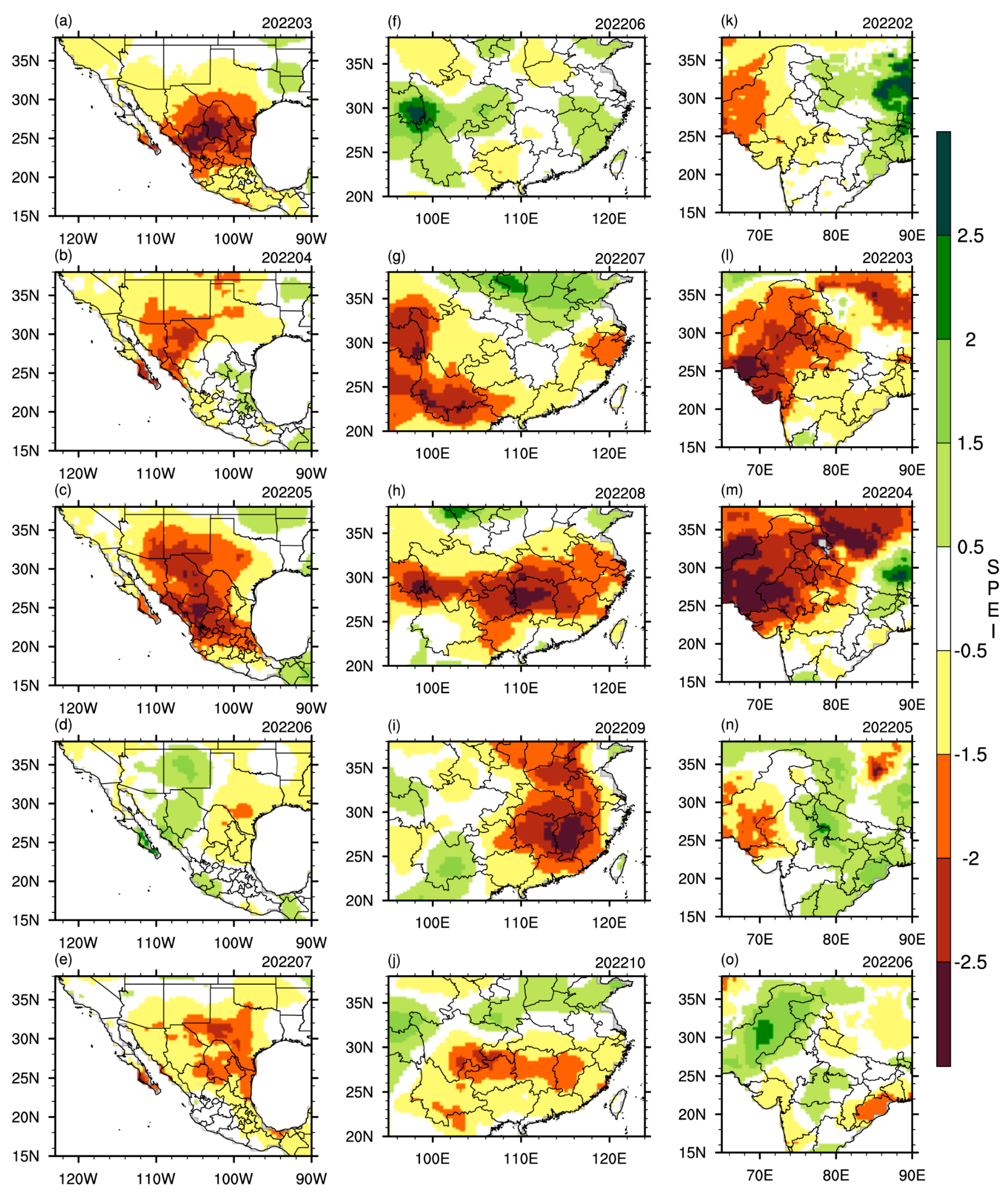
5.3. Drought Case Studies

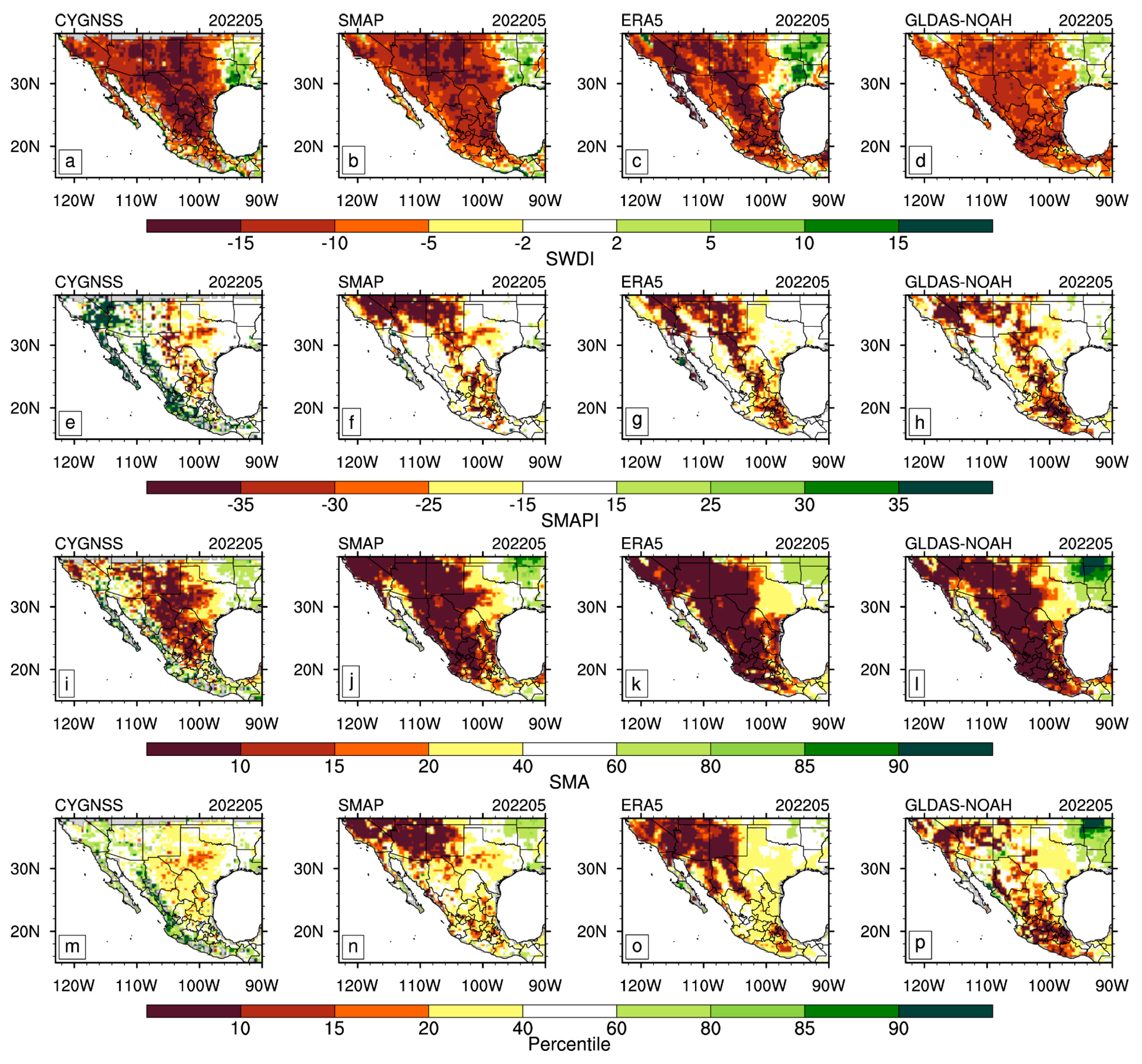
Severe drought events exhibit distinct spatial patterns. In this section, we highlight three extreme drought cases from different regions to illustrate the performance of various drought indicators derived from different soil moisture datasets in depicting these events. In the summer of 2022, southern China experienced prolonged and severe drought conditions, spanning both summer and autumn. The drought, characterized by a wide spatial extent, long duration, and high intensity, peaked in August 2022. This prolonged period of high temperatures and drought significantly impacted agricultural production, water resources, energy supply, and human health in the Yangtze River Basin and its southern regions. Moreover, it adversely affected the local ecosystem. Simultaneously, during the first half of 2022, North America endured intense and consecutive heatwaves, with some regions experiencing daily maximum temperatures exceeding 45 °C. These high-temperature heatwaves exacerbated drought development, with the most extensive and intense drought observed in May, as indicated by the SPEI results (Figure 23a–e). In March and April 2022, India and Pakistan faced severe heat waves, resulting in March being the hottest in India since 1901. These conditions persisted through April, affecting large parts of northwestern India. To delve into these events, we illustrate their drought progression and resolution based on the SPEI in Figure 23. This representation highlights the peak periods of these drought events in May (North America), August (southern China), and April 2022 (India and Pakistan). In comparison, we present the drought conditions from different drought indicators derived from various soil moisture datasets for North America in May 2022 (Figure 24), southern China in August 2022 (Figure 25), and India and Pakistan in April 2022 (Figure 26).

The drought patterns in North America during May 2022 are depicted by various drought indicators derived from different soil moisture datasets in Figure 24. Severe drought events (shown in red) identified with the SWDI and SMA align closely but are larger with the patterns identified with the SPEI. However, areas identified with the SMAPI and Percentile are comparatively smaller and have the wrong spatial structure compared with the SPEI. The results from CYGNSS, apart from the SWDI, demonstrate smaller areas and weaker intensity across other drought indices compared with the other three datasets, indicating its limited performance in describing this specific drought event.

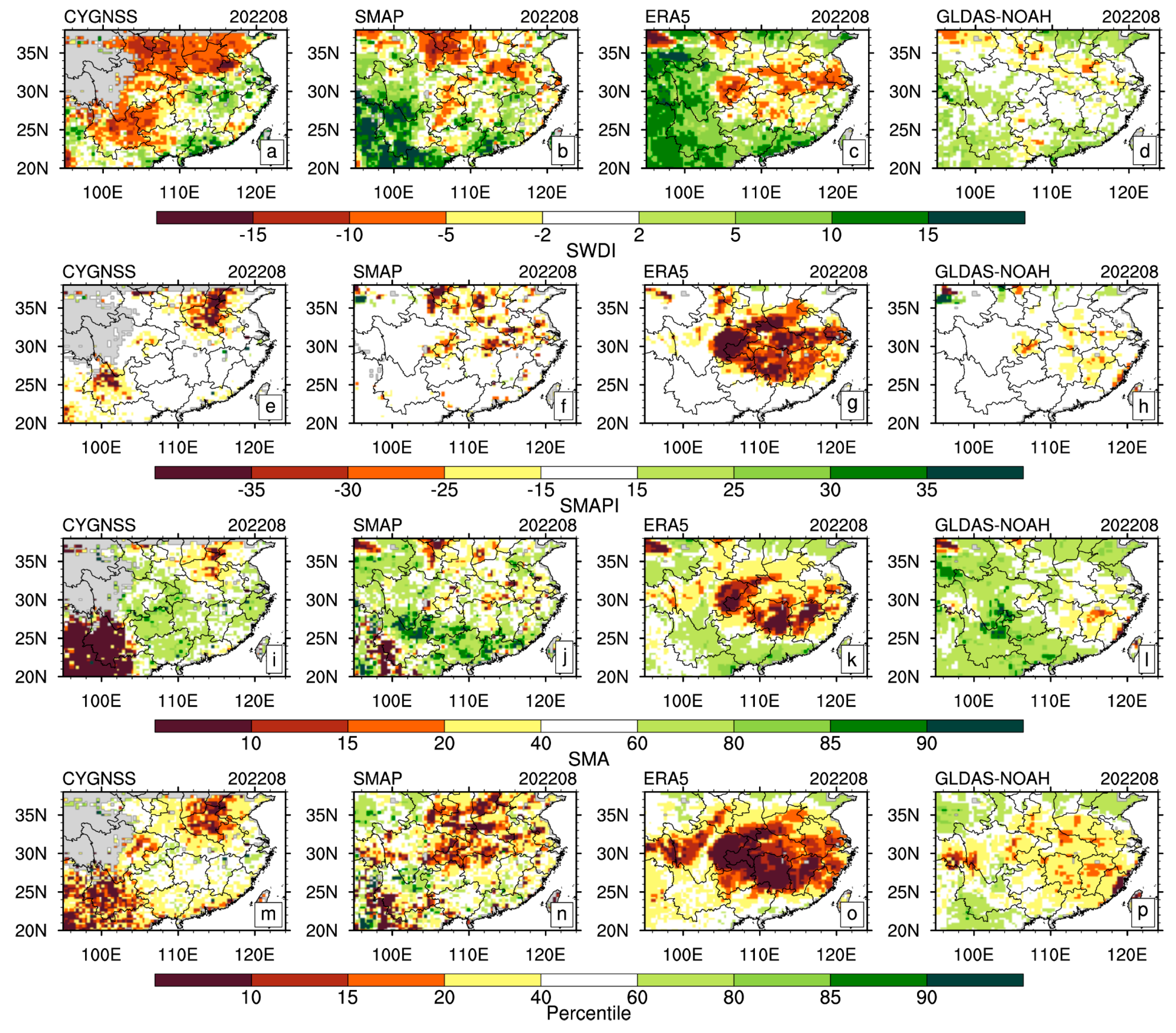
The drought conditions prevalent in southern China in August 2022 are shown in Figure 25. In general, the drought event as represented by diverse drought indicators and soil moisture datasets exhibits a relatively confined geographic extent and limited intensity. Among the datasets, ERA5 consistently yields the most robust results across various drought indicators. It demonstrates remarkable performance, particularly evident in the Percentile index, where it outperforms the SPEI results. In contrast, the performance of the CYGNSS dataset across different drought indicators is notably less effective in capturing the intensity and spatial scope of this specific drought event.

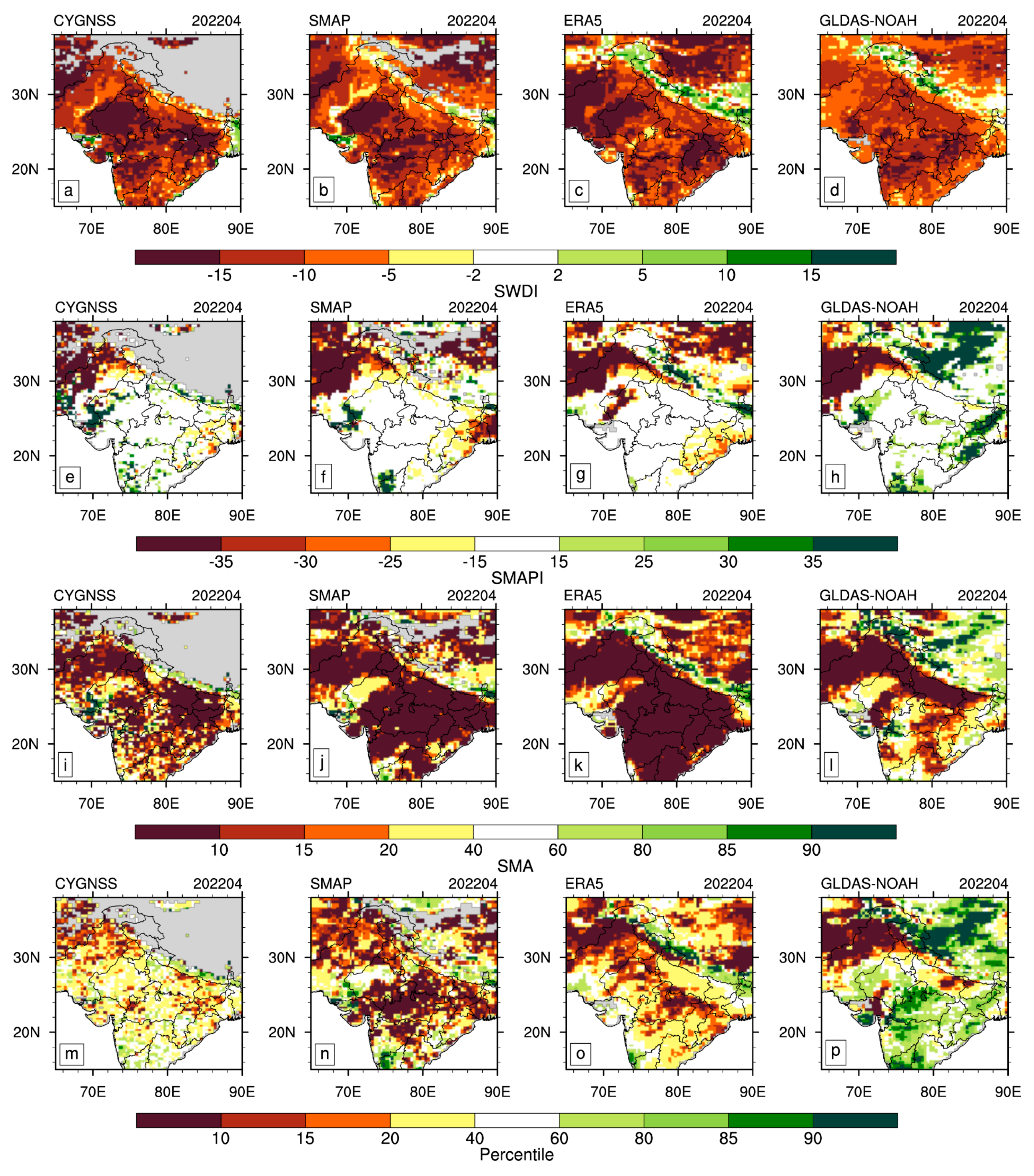
The April 2022 drought affecting India and Pakistan is well replicated by the SWDI across various datasets, as illustrated in Figure 26a–d. However, results from alternative drought indicators and datasets typically portray a comparatively reduced extent and intensity in relation to the SPEI-based findings. The SMA-based results exhibit variations in the range and location of drought occurrence for ERA5 and SMAP (Figure 26j,k). Relative to other datasets, CYGNSS is better equipped to depict drought conditions with the SWDI indicator, although it tends to be suboptimal when utilizing alternative drought indicators, as it typically portrays a limited intensity and spatial extent of drought events.

6. Discussion

The comparative analysis of CYGNSS soil moisture data with SMAP, ERA5, and GLDAS-NOAH indicates that CYGNSS exhibits distinctive temporal coverage variations across regions, with limitations in equatorial rainforests and the Tibetan Plateau. The spatial patterns of the averages and standard deviation in the soil moisture reveal consistent structures across the datasets. However, notable differences in absolute values are observed, especially in regions like the Amazon Basin, southern China, and Southeast Asia. CYGNSS tends to exhibit smaller values in certain regions compared with the other datasets, suggesting potential biases. The standard deviation analysis demonstrates distinct variability patterns, with CYGNSS presenting unique characteristics in specific regions. Examining the influence of climate and land cover on data disparities reveals nuanced relationships. Correlation coefficients and RMSE values vary across climate types, emphasizing the impact of specific climate conditions on soil moisture accuracy. These features of CYGNSS are crucial for interpreting soil moisture dynamics across diverse geographic contexts and are helpful for improving the inversion of soil moisture from CYGNSS data.

When assessing the performance of drought indicators derived from various soil moisture datasets, our study focused on drought percentage and intensity. The drought indicator highlights prolonged water scarcity in desert areas, grasslands, and specific regions such as the Sahara Desert, Arabian Desert, South African grasslands, and parts of Australia. CYGNSS data exhibit broader and more intense long-term drought conditions compared with other datasets, especially in desert areas. However, regions with low drought occurrence are identified in the Amazon River Basin, equatorial Africa, eastern North America, southern China, and Southeast Asia. The drought intensity analysis revealed consistent spatial patterns across all datasets, with higher intensity observed in the Sahara Desert and Arabian regions. However, CYGNSS consistently identifies more regions without significant drought. The performance of drought indicators from CYGNSS showcases the importance of improving the accuracy of CYGNSS data.

The comparison of drought indicators with the SPEI displays some description of their efficacy. Spatial correlations between the SWDI, SMAPI, SMA, and Percentile with the SPEI indicate strong correlations for drought percentage, particularly with ERA5. CYGNSS exhibits notable spatial structures and correlation coefficients, though its performance varies across regions. In describing severe drought events, CYGNSS, while exhibiting similarities with other datasets, may demonstrate reduced scores in specific regions, which emphasizes the need for cautious interpretation. The case studies of severe drought events in southern China, North America, and India/Pakistan illustrate the performance of different drought indicators. CYGNSS tends to depict smaller areas and weaker intensities across various drought indices compared with the other datasets. The soil moisture data from ERA5 usually exhibit a better performance in describing drought in almost all drought indicators. This may be due to its generation process, which assimilates meteorological information such as observation precipitation. Thus, in order to improve the accuracy of CYGNSS soil moisture retrievals, it is necessary to introduce meteorological elements, especially precipitation, into the generation process.

7. Conclusions

In this study, we conducted a comprehensive analysis of CYGNSS satellite soil moisture data spanning from 1 January 2018 to 31 December 2022, comparing them with the SMAP, ERA5, and GLDAS-NOAH datasets. Our analysis revealed that CYGNSS exhibited similar spatial patterns in the mean soil moisture and standard deviation compared with the other datasets. However, CYGNSS displayed a relatively smaller standard deviation in most studied regions. The relationship between CYGNSS and other datasets varied across different climate and land cover types. Specifically, CYGNSS exhibited the strongest correlation with SMAP, followed by ERA5. This relationship was significantly influenced by CYGNSS’s own standard deviation. Higher standard deviations led to higher correlation coefficients. Additionally, the average RMSE was related to CYGNSS’s mean soil moisture values, indicating that larger average values led to higher RMSE values. These relationships underscore the importance of accounting for diverse climate and land cover types when interpreting CYGNSS soil moisture data.

To assess CYGNSS’s ability to characterize drought, we constructed four drought indicators (the SWDI, SMAPI, SMA, and Percentile) using the CYGNSS, SMAP, ERA5, and GLDAS-NOAH soil moisture datasets. These indicators were then compared with the SPEI index on a monthly scale. The results demonstrated that CYGNSS soil moisture data exhibited drought characterization abilities. The spatial patterns of drought characteristics, such as the drought percentage and average intensity, presented by CYGNSS using different drought indicators were comparable to those of the other soil moisture datasets. However, the recognition skill for severe drought events was relatively weak for all datasets, with CYGNSS performing the least effectively and ERA5 exhibiting the highest skill.

In an effort to construct drought indicators based on long-term soil moisture anomalies, we corrected the CYGNSS soil moisture data with the cumulative distribution function. Although the performance of the resulting drought indicators (the SMAPI, SMA, and Percentile) after correction was comparable to that of the SWDI, and the comparison results of the drought event descriptions were consistent, there is still room for improvement. Future research directions could involve correcting soil moisture data based on site-specific observations to enhance accuracy. Additionally, we recommend exploring the weekly or pentad characteristics of drought indicators to provide a more detailed understanding of drought occurrence and development.

This study shows the potential and limitations of CYGNSS satellite soil moisture data in characterizing drought events. While CYGNSS shows promise, addressing its limitations via further calibration and considering different temporal scales will enhance its applicability in drought monitoring and prediction. The findings from this study contribute to our understanding of the evolving landscape of satellite-based soil moisture data and their utility in drought analysis.

References

1. Yuan, X.; Wang, Y.; Ji, P.; Wu, P.; Sheffield, J.; Otkin, J.A. A Global Transition to Flash Droughts under Climate Change. Science 2023, 380, 187–191. [Google Scholar] [CrossRef] [PubMed]
2. Dai, A. Drought under Global Warming: A Review. WIREs Clim. Change 2011, 2, 45–65. [Google Scholar] [CrossRef]
3. Mishra, A.K.; Singh, V.P. A Review of Drought Concepts. J. Hydrol. 2010, 391, 202–216. [Google Scholar] [CrossRef]
4. Saha, A.; Pal, S.C.; Chowdhuri, I.; Roy, P.; Chakrabortty, R.; Shit, M. Vulnerability Assessment of Drought in India: Insights from Meteorological, Hydrological, Agricultural and Socio-Economic Perspectives. Gondwana Res. 2022, 123, 68–88. [Google Scholar] [CrossRef]
5. Haile, G.G.; Tang, Q.; Li, W.; Liu, X.; Zhang, X. Drought: Progress in Broadening Its Understanding. WIREs Water 2020, 7, e1407. [Google Scholar] [CrossRef]
6. Wilhite, D.A.; Glantz, M.H. Understanding: The Drought Phenomenon: The Role of Definitions. Water Int. 1985, 10, 111–120. [Google Scholar] [CrossRef]
7. Liu, X.; Zhu, X.; Pan, Y.; Li, S.; Liu, Y.; Ma, Y. Agricultural Drought Monitoring: Progress, Challenges, and Prospects. J. Geogr. Sci. 2016, 26, 750–767. [Google Scholar] [CrossRef]
8. Javed, T.; Li, Y.; Rashid, S.; Li, F.; Hu, Q.; Feng, H.; Chen, X.; Ahmad, S.; Liu, F.; Pulatov, B. Performance and Relationship of Four Different Agricultural Drought Indices for Drought Monitoring in China’s Mainland Using Remote Sensing Data. Sci. Total Environ. 2021, 759, 143530. [Google Scholar] [CrossRef]
9. Chatterjee, S.; Desai, A.R.; Zhu, J.; Townsend, P.A.; Huang, J. Soil Moisture as an Essential Component for Delineating and Forecasting Agricultural Rather than Meteorological Drought. Remote Sens. Environ. 2022, 269, 112833. [Google Scholar] [CrossRef]
10. Sheffield, J.; Goteti, G.; Wen, F.; Wood, E.F. A Simulated Soil Moisture Based Drought Analysis for the United States. J. Geophys. Res. Atmos. 2004, 109, D24108. [Google Scholar] [CrossRef]
11. Afshar, M.H.; Bulut, B.; Duzenli, E.; Amjad, M.; Yilmaz, M.T. Global Spatiotemporal Consistency between Meteorological and Soil Moisture Drought Indices. Agric. For. Meteorol. 2022, 316, 108848. [Google Scholar] [CrossRef]
12. Xu, L.; Abbaszadeh, P.; Moradkhani, H.; Chen, N.; Zhang, X. Continental Drought Monitoring Using Satellite Soil Moisture, Data Assimilation and an Integrated Drought Index. Remote Sens. Environ. 2020, 250, 112028. [Google Scholar] [CrossRef]
13. West, H.; Quinn, N.; Horswell, M. Remote Sensing for Drought Monitoring & Impact Assessment: Progress, Past Challenges and Future Opportunities. Remote Sens. Environ. 2019, 232, 111291. [Google Scholar] [CrossRef]
14. AghaKouchak, A.; Farahmand, A.; Melton, F.S.; Teixeira, J.; Anderson, M.C.; Wardlow, B.D.; Hain, C.R. Remote Sensing of Drought: Progress, Challenges and Opportunities. Rev. Geophys. 2015, 53, 452–480. [Google Scholar] [CrossRef]
15. Zhou, H.; Geng, G.; Yang, J.; Hu, H.; Sheng, L.; Lou, W. Improving Soil Moisture Estimation via Assimilation of Remote Sensing Product into the DSSAT Crop Model and Its Effect on Agricultural Drought Monitoring. Remote Sens. 2022, 14, 3187. [Google Scholar] [CrossRef]
16. Vreugdenhil, M.; Greimeister-Pfeil, I.; Preimesberger, W.; Camici, S.; Dorigo, W.; Enenkel, M.; van der Schalie, R.; Steele-Dunne, S.; Wagner, W. Microwave Remote Sensing for Agricultural Drought Monitoring: Recent Developments and Challenges. Front. Water 2022, 4, 1045451. [Google Scholar] [CrossRef]
17. Dorigo, W.; Wagner, W.; Albergel, C.; Albrecht, F.; Balsamo, G.; Brocca, L.; Chung, D.; Ertl, M.; Forkel, M.; Gruber, A.; et al. ESA CCI Soil Moisture for Improved Earth System Understanding: State-of-the Art and Future Directions. Remote Sens. Environ. 2017, 203, 185–215. [Google Scholar] [CrossRef]
18. Jung, C.; Lee, Y.; Cho, Y.; Kim, S. A Study of Spatial Soil Moisture Estimation Using a Multiple Linear Regression Model and MODIS Land Surface Temperature Data Corrected by Conditional Merging. Remote Sens. 2017, 9, 870. [Google Scholar] [CrossRef]
19. Babaeian, E.; Sadeghi, M.; Jones, S.B.; Montzka, C.; Vereecken, H.; Tuller, M. Ground, Proximal, and Satellite Remote Sensing of Soil Moisture. Rev. Geophys. 2019, 57, 530–616. [Google Scholar] [CrossRef]
20. Kerr, Y.H. Soil Moisture from Space: Where Are We? Hydrogeol. J. 2007, 15, 117–120. [Google Scholar] [CrossRef]
21. Martínez-Fernández, J.; González-Zamora, A.; Sánchez, N.; Gumuzzio, A.; Herrero-Jiménez, C.M. Satellite Soil Moisture for Agricultural Drought Monitoring: Assessment of the SMOS Derived Soil Water Deficit Index. Remote Sens. Environ. 2016, 177, 277–286. [Google Scholar] [CrossRef]
22. Sadri, S.; Wood, E.F.; Pan, M. Developing a Drought-Monitoring Index for the Contiguous US Using SMAP. Hydrol. Earth Syst. Sci. 2018, 22, 6611–6626. [Google Scholar] [CrossRef]
23. Mishra, A.; Vu, T.; Veettil, A.V.; Entekhabi, D. Drought Monitoring with Soil Moisture Active Passive (SMAP) Measurements. J. Hydrol. 2017, 552, 620–632. [Google Scholar] [CrossRef]
24. Sadri, S.; Pan, M.; Wada, Y.; Vergopolan, N.; Sheffield, J.; Famiglietti, J.S.; Kerr, Y.; Wood, E. A Global Near-Real-Time Soil Moisture Index Monitor for Food Security Using Integrated SMOS and SMAP. Remote Sens. Environ. 2020, 246, 111864. [Google Scholar] [CrossRef]
25. Liu, Y.; Liu, Y.; Wang, W. Inter-Comparison of Satellite-Retrieved and Global Land Data Assimilation System-Simulated Soil Moisture Datasets for Global Drought Analysis. Remote Sens. Environ. 2019, 220, 1–18. [Google Scholar] [CrossRef]
26. Champagne, C.; McNairn, H.; Berg, A.A. Monitoring Agricultural Soil Moisture Extremes in Canada Using Passive Microwave Remote Sensing. Remote Sens. Environ. 2011, 115, 2434–2444. [Google Scholar] [CrossRef]
27. Cao, M.; Chen, M.; Liu, J.; Liu, Y. Assessing the Performance of Satellite Soil Moisture on Agricultural Drought Monitoring in the North China Plain. Agric. Water Manag. 2022, 263, 107450. [Google Scholar] [CrossRef]
28. Shangguan, W.; Zhang, R.; Li, L.; Zhang, S.; Zhang, Y.; Huang, F.; Li, J.; Liu, W. Assessment of Agricultural Drought Based on Reanalysis Soil Moisture in Southern China. Land 2022, 11, 502. [Google Scholar] [CrossRef]
29. Fang, B.; Kansara, P.; Dandridge, C.; Lakshmi, V. Drought Monitoring Using High Spatial Resolution Soil Moisture Data over Australia in 2015–2019. J. Hydrol. 2021, 594, 125960. [Google Scholar] [CrossRef]
30. Carreno-Luengo, H.; Crespo, J.A.; Akbar, R.; Bringer, A.; Warnock, A.; Morris, M.; Ruf, C. The CYGNSS Mission: On-Going Science Team Investigations. Remote Sens. 2021, 13, 1814. [Google Scholar] [CrossRef]
31. Clarizia, M.P.; Pierdicca, N.; Costantini, F.; Floury, N. Analysis of CYGNSS Data for Soil Moisture Retrieval. IEEE J. Sel. Top. Appl. Earth Obs. Remote Sens. 2019, 12, 2227–2235. [Google Scholar] [CrossRef]
32. Senyurek, V.; Lei, F.; Boyd, D.; Kurum, M.; Gurbuz, A.C.; Moorhead, R. Machine Learning-Based CYGNSS Soil Moisture Estimates over ISMN Sites in CONUS. Remote Sens. 2020, 12, 1168. [Google Scholar] [CrossRef]
33. Chew, C.; Small, E. Description of the UCAR/CU Soil Moisture Product. Remote Sens. 2020, 12, 1558. [Google Scholar] [CrossRef]
34. Yang, T.; Wan, W.; Sun, Z.; Liu, B.; Li, S.; Chen, X. Comprehensive evaluation of using TechDemoSat-1 and CYGNSS data to estimate soil moisture over mainland China. Remote Sens. 2020, 12, 1699. [Google Scholar] [CrossRef]
35. Wang, H.; Yuan, Q.; Zhao, H.; Xu, H. In-situ and triple-collocation based assessments of CYGNSS-R soil moisture compared with satellite and merged estimates quasi-globally. J. Hydrol. 2022, 615, 128716. [Google Scholar] [CrossRef]
36. Dong, Z.; Jin, S.; Li, L.; Wang, P. Validation of CYGNSS soil moisture products using in situ measurements: A case study of Southern China. Theor. Appl. Climatol. 2023, 153, 1085–1103. [Google Scholar] [CrossRef]
37. Entekhabi, D.; Njoku, E.G.; O’Neill, P.E.; Kellogg, K.H.; Crow, W.T.; Edelstein, W.N.; Entin, J.K.; Goodman, S.D.; Jackson, T.J.; Johnson, J.; et al. The Soil Moisture Active Passive (SMAP) Mission. Proc. IEEE 2010, 98, 704–716. [Google Scholar] [CrossRef]
38. Muñoz-Sabater, J.; Dutra, E.; Agustí-Panareda, A.; Albergel, C.; Arduini, G.; Balsamo, G.; Boussetta, S.; Choulga, M.; Harrigan, S.; Hersbach, H.; et al. ERA5-Land: A State-of-the-Art Global Reanalysis Dataset for Land Applications. Earth Syst. Sci. Data 2021, 13, 4349–4383. [Google Scholar] [CrossRef]
39. Rodell, M.; Houser, P.R.; Jambor, U.; Gottschalck, J.; Mitchell, K.; Meng, C.-J.; Arsenault, K.; Cosgrove, B.; Radakovich, J.; Bosilovich, M.; et al. The Global Land Data Assimilation System. Bull. Am. Meteorol. Soc. 2004, 85, 381–394. [Google Scholar] [CrossRef]
40. Beck, H.E.; Zimmermann, N.E.; McVicar, T.R.; Vergopolan, N.; Berg, A.; Wood, E.F. Present and Future Köppen-Geiger Climate Classification Maps at 1-Km Resolution. Sci. Data 2018, 5, 180214. [Google Scholar] [CrossRef]
41. Friedl, M.; Sulla-Menashe, D. MODIS/Terra+ Aqua Land Cover Type Yearly L3 Global 500m SIN Grid V061. NASA EOSDIS Land; Processes DAAC: Sioux Falls, SD, USA, 2022. [Google Scholar]
42. Vicente-Serrano, S.M.; Beguería, S.; López-Moreno, J.I.; Angulo, M.; Kenawy, A.E. A New Global 0.5° Gridded Dataset (1901–2006) of a Multiscalar Drought Index: Comparison with Current Drought Index Datasets Based on the Palmer Drought Severity Index. J. Hydrometeorol. 2010, 11, 1033–1043. [Google Scholar] [CrossRef]
43. Vicente-Serrano, S.M.; Beguería, S.; López-Moreno, J.I. A Multiscalar Drought Index Sensitive to Global Warming: The Standardized Precipitation Evapotranspiration Index. J. Clim. 2010, 23, 1696–1718. [Google Scholar] [CrossRef]
44. Martínez-Fernández, J.; González-Zamora, A.; Sánchez, N.; Gumuzzio, A. A Soil Water Based Index as a Suitable Agricultural Drought Indicator. J. Hydrol. 2015, 522, 265–273. [Google Scholar] [CrossRef]
45. Saxton, K.E.; Rawls, W.J. Soil Water Characteristic Estimates by Texture and Organic Matter for Hydrologic Solutions. Soil Sci. Soc. Am. J. 2006, 70, 1569–1578. [Google Scholar] [CrossRef]
46. Hengl, T.; de Jesus, J.M.; Heuvelink, G.B.M.; Gonzalez, M.R.; Kilibarda, M.; Blagotić, A.; Shangguan, W.; Wright, M.N.; Geng, X.; Bauer-Marschallinger, B.; et al. SoilGrids250m: Global Gridded Soil Information Based on Machine Learning. PLoS ONE 2017, 12, e0169748. [Google Scholar] [CrossRef] [PubMed]
47. Brocca, L.; Ciabatta, L.; Massari, C.; Moramarco, T.; Hahn, S.; Hasenauer, S.; Kidd, R.; Dorigo, W.; Wagner, W.; Levizzani, V. Soil as a Natural Rain Gauge: Estimating Global Rainfall from Satellite Soil Moisture Data. J. Geophys. Res. Atmos. 2014, 119, 5128–5141. [Google Scholar] [CrossRef]
48. Vroege, W.; Bucheli, J.; Dalhaus, T.; Hirschi, M.; Finger, R. Insuring Crops from Space: The Potential of Satellite-Retrieved Soil Moisture to Reduce Farmers’ Drought Risk Exposure. Eur. Rev. Agric. Econ. 2021, 48, 266–314. [Google Scholar] [CrossRef]
49. Reichle, R.H.; Koster, R.D. Bias Reduction in Short Records of Satellite Soil Moisture. Geophys. Res. Lett. 2004, 31, L19501. [Google Scholar] [CrossRef]
50. Draper, C.S.; Walker, J.P.; Steinle, P.J.; de Jeu, R.A.M.; Holmes, T.R.H. An Evaluation of AMSR–E Derived Soil Moisture over Australia. Remote Sens. Environ. 2009, 113, 703–710. [Google Scholar] [CrossRef]
51. Singh, A.; Gaurav, K.; Meena, G.K.; Kumar, S. Estimation of Soil Moisture Applying Modified Dubois Model to Sentinel-1; A Regional Study from Central India. Remote Sens. 2020, 12, 2266. [Google Scholar] [CrossRef]
52. Wilks, D.S. Statistical Methods in the Atmospheric Sciences; Academic Press: Cambridge, MA, USA, 2011; Volume 100. [Google Scholar]
53. Jolliffe, I.T.; Stephenson, D.B. (Eds.) Forecast Verification: A Practitioner’s Guide in Atmospheric Science; John Wiley & Sons: Hoboken, NJ, USA, 2012. [Google Scholar]
Figure 1. Köppen–Geiger climate classification (a) and land cover types from the MODIS Terra+Aqua combined land cover product (MCD12C1v061) (b) in the investigated region. In the climate classification (a), distinct codes represent various climatic zones: Af (tropical rainforest), Am (tropical monsoon), Aw (tropical savanna), BW (arid desert), BS (arid steppe), Cs (temperate dry summer), Cw (temperate dry winter), Cf (temperate and no dry season), and DE (cold or polar). Land cover types (b) encompass forests (evergreen needleleaf forest, evergreen broadleaf forest, deciduous broadleaf forest, and mixed forest), shrublands (closed shrubland and open shrubland), savannas (woody savannas and savannas), grasslands, croplands (permanent wetlands, croplands, urban and built-up areas, cropland/natural vegetation mosaic, and snow and ice cover), and barren lands (barren or sparsely vegetated areas). This comprehensive categorization provides a foundation for our in-depth analysis of the region’s ecological and climatic intricacies. The four white dots in the figure indicate the specified location used in Figure 4.
Remotesensing 16 00116 g001
Figure 2. The proportion of daily data volume from (a) CYGNSS and (b) SMAP from 1 January 2018 to 31 December 2022, totaling 1825 days.
Remotesensing 16 00116 g002
Figure 3. The spatial patterns of average daily soil moisture levels from (a) CYGNSS, (b) SMAP, (c) ERA5, and (d) GLDAS_NOAH, along with the corresponding standard deviations depicted in panels (eh). The data span from 1 January 2018 to 31 December 2022.
Remotesensing 16 00116 g003
Figure 4. The mean daily time series of soil moisture at four specified locations from CYGNSS (in red), SMAP (in blue), ERA5-land (in green), and GLDAS-NOAH (in purple). The data span from 2018 to 2022 and are averaged over each day of the year. The longitude and latitude coordinates for each location are provided in the upper left corner of the respective panel.
Remotesensing 16 00116 g004
Figure 5. Correlation analysis of daily soil moisture data from CYGNSS, SMAP, ERA5, and GLDAS_NOAH from 1 January 2018 to 31 December 2022. The datasets used for calculating the correlations are indicated in the upper left corner of each panel: (a) is the correlation between CYGNSS and SMAP, (b) between CYGNSS and ERA5, (c) between CYGNSS and GLDAS_NOAH, (d) between SMAP and ERA5, (e) between SMAP and GLDAS_NOAH, (f) between EAR5 and GLDAS_NOAH.
Remotesensing 16 00116 g005
Figure 6. Root-mean-square error (RMSE) values representing the disparity between the daily soil moisture datasets of CYGNSS, SMAP, ERA5, and GLDAS_NOAH, observed from 1 January 2018 to 31 December 2022. The upper left corner of each panel denotes the datasets employed for calculating the RMSE values: (a) is between CYGNSS and SMAP, (b) between CYGNSS and ERA5, (c) between CYGNSS and GLDAS_NOAH, (d) between SMAP and ERA5, (e) between SMAP and GLDAS_NOAH, (f) between EAR5 and GLDAS_NOAH.
Remotesensing 16 00116 g006
Figure 7. The distributions of correlation (a) and root-mean-square error (RMSE) (b) values based on different Köppen-Geiger climate classifications for various data pairs. The distributions are depicted with dashed lines representing the 95th and 5th percentile values, box lines denoting the interquartile range encompassing the 75th and 25th percentile values, and horizontal lines indicating the average values within each classification.
Remotesensing 16 00116 g007
Figure 8. The same as Figure 7a,b but for different land cover types.
Remotesensing 16 00116 g008
Figure 9. (ad) Drought percentage (%) and (eh) drought severity analysis based on the Soil Water Deficit Index (SWDI) derived from CYGNSS, SMAP, ERA5, and GLDAS-NOAH datasets spanning from January 2018 to December 2022.
Remotesensing 16 00116 g009
Figure 10. The same as Figure 9 but based on the Soil Moisture Anomaly Percentage Index (SMAPI).
Remotesensing 16 00116 g010
Figure 11. The same as Figure 9a–h but based on the Soil Moisture Anomaly (SMA).
Remotesensing 16 00116 g011
Figure 12. The same as Figure 9a–h but based on the Soil Moisture Percentile (Percentile).
Remotesensing 16 00116 g012
Figure 13. (a) Drought percentage (%) and (b) drought severity based on the Standardized Precipitation Evapotranspiration Index (SPEI). The selected drought scenario is defined as SPEI values below −1.5.
Remotesensing 16 00116 g013
Figure 14. Spatial correlation coefficients of (a) drought percentage and (b) drought intensity between SPEI and different soil-moisture-based drought indicators.
Remotesensing 16 00116 g014
Figure 15. Correlation analysis between the Standardized Precipitation Evapotranspiration Index (SPEI) and the Soil Water Deficit Index (SWDI) derived from CYGNSS (a), SMAP (b), ERA5 (c), and GLDAS-NOAH (d) from January 2018 to December 2022.
Remotesensing 16 00116 g015
Figure 16. The same as Figure 15a–d but between the Standardized Precipitation Evapotranspiration Index (SPEI) and the Soil Moisture Anomaly Percentage Index (SMAPI).
Remotesensing 16 00116 g016
Figure 17. The same as Figure 15a–d but between the Standardized Precipitation Evapotranspiration Index (SPEI) and the Soil Moisture Anomaly (SMA).
Remotesensing 16 00116 g017
Figure 18. The same as Figure 15a–d but between the Standardized Precipitation Evapotranspiration Index (SPEI) and the Soil Moisture Percentile.
Remotesensing 16 00116 g018
Figure 19. Evaluation metrics for severe drought events: (ad) total score (TS), (eh) hit rate (HR), (il) miss rate (MR), and (mp) false alarm rate (FAR) obtained from SWDI analysis of the CYGNSS, SMAP, ERA5, and GLDAS-NOAH datasets compared with results identified with SPEI from January 2018 to December 2022.
Remotesensing 16 00116 g019
Figure 20. The same as Figure 19a–p but from SMAPI.
Remotesensing 16 00116 g020
Figure 21. The same as Figure 19a–p but from SMA.
Remotesensing 16 00116 g021
Figure 22. The same as Figure 19a–p but from Percentile.
Remotesensing 16 00116 g022
Figure 23. Drought event development process depicted by the Standardized Precipitation Evapotranspiration Index (SPEI) across North America from March to July (ae), southern China from June to October 2022 (fj), and India and Pakistan from February to June 2022 (ko). (c,h,m) denote the peaks of these drought events.
Remotesensing 16 00116 g023
Figure 24. Drought conditions represented by SWDI (ad), SMAPI (eh), SMA (il), and Percentile (mp) using diverse soil moisture datasets across North America in May 2022. The datasets are organized as follows: first column—CYGNSS dataset; second column—SMAP; third column—ERA5; and fourth column—GLDAS-NOAH.
Remotesensing 16 00116 g024
Figure 25. The same as Figure 24a–p but across southern China in August 2022.
Remotesensing 16 00116 g025
Figure 26. The same as Figure 24a–p but across India and Pakistan in April 2022.
Remotesensing 16 00116 g026