Abstract
The characterization of landslides located in remote areas poses significant challenges due to the costs of reaching the sites and the lack of reliable subsurface data to constrain geological interpretations. In this paper, the advantages of combining field and remote sensing techniques to investigate the deformation and stability of rock slopes are demonstrated. The characterization of the Fels landslide, a large, slowly deforming rock slope in central Alaska, is described. Historical aerial imagery is used to highlight the relationship between glacier retreat and developing instability. Airborne laser scanning (ALS) and Structure-from-Motion (SfM) datasets are used to investigate the structural geological setting of the landslide, revealing a good agreement between structural discontinuities at the outcrop and slope scales. The magnitude, plunge, and direction of slope surface displacements and their changes over time are studied using a multi-temporal synthetic aperture radar speckle-tracking (SAR ST) dataset. The analyses show an increase in displacement rates (i.e., an acceleration of the movement) between 2010 and 2020. Significant spatial variations of displacement direction and plunge are noted and correlated with the morphology of the failure surface reconstructed using the vector inclination method (VIM). In particular, steeper displacement vectors were reconstructed in the upper slope, compared to the central part, thus suggesting a change in basal surface morphology, which is largely controlled by rock mass foliation. Through this analytical approach, the Fels landslide is shown to be a slow-moving, compound rockslide, the displacement of which is controlled by structural geological features and promoted by glacier retreat.
1. Introduction
Landslides pose a threat to nearby communities and infrastructure and can have significant social and economic consequences [1]. Highways, railroads, and pipelines in alpine areas are especially vulnerable to landslide damage due to the location and extent of such linear infrastructure near or at valley floors and adjacent to steep slopes. Damage or blockage of linear infrastructure interrupts the movement of people and goods and can, in some cases, isolate remote communities [2]. The characterization and monitoring of unstable rock slopes is, therefore, critical to ensuring the safety of people, infrastructure, and communities.
However, the investigation of unstable rock slopes, particularly those in remote regions, is often challenging due to difficulties in access and safety on the ground. In such cases, remote sensing techniques can be employed to collect geological data required to assess the state of activity of the slope and to identify the underlying structural, geomechanical, and geomorphic factors and processes responsible for instability.
Terrestrial and airborne laser scanning (TLS and ALS) methods involve the emission of a laser pulse from an instrument, referred to as a laser scanner, and the measurement of the time required for the pulse to reach a sensor mounted on the same instrument after bouncing off the object surface [3]. Such a process, repeated several thousand times per second, allows high-resolution 3D models of the ground surface to be collected in the form of point clouds. The models can then be used to perform discontinuity mapping, rock mass characterization, and slope surface analysis [4,5]. High-frequency sampling of the reflected signal allows a researcher to identify multiple returns for each emitted pulse and enables the removal of vegetation and other minor obstacles in order to create a so-called “bare earth” dataset. Surface features of interest (e.g., cracks, grabens, gullies, fractures) can thus be readily identified and interpreted across heavily vegetated slopes (e.g., [6]). Because such surveys are accurate and can be repeated, both TLS and ALS are now widely used to characterize and monitor unstable slopes (e.g., [7,8,9]).
Digital photogrammetric techniques such as Unmanned Aerial Vehicle-based Structure-from-Motion (UAV-SfM) are capable of reconstructing the 3D geometry of a scene or an object using pairs or groups of digital photographs and are therefore routinely employed to analyze and characterize deforming slopes at a variety of scales [5,7,10,11]. To a more limited extent, these techniques have been exploited to monitor rock slope deformation and landslide displacement [12,13]. Photogrammetric methods take advantage of the concept of “stereoscopic parallax”, which is the relative change in the position of a pixel or feature in photographs taken from different positions. Positions within the 3D space of common features are then precisely determined by comparing their position in the photographs and successively computing, through an iterative process, positions of camera stations (i.e., the position from which each photo was taken) relative to the investigated scene [14,15].
Recently, 3D and 2D datasets have been integrated, enhancing the amount and quality of geological, geomechanical, and hydrogeological data when analyzing rock slopes. In particular, infrared thermography (IRT) datasets, gathered in tandem with TLS datasets, have been used to investigate the degree of fracturing [16] and rock mass quality [17] within rock slopes. To a lesser extent, hyperspectral imagery has also been incorporated with 3D datasets to map lithological changes within quarry walls, exploiting the varied different spectral responses of minerals [18].
A limitation of both laser scanners and photogrammetric surveys is the need to travel to the study site (for ground-based surveys) or fly over it (for airborne surveys) to collect high-resolution data. Repeated flights and travel to a site can be costly but may be required for rock slope monitoring purposes. Alternatively, TLS can be installed at the site to allow for quasi-real-time monitoring of limited sections of rock slopes by automatically repeating the scan at defined intervals [19,20]. Multiple fixed camera systems have also been employed to perform high-temporal-resolution monitoring of sections of rock slopes using the SfM technique [21]. In all cases, however, high-spatial-resolution and high-temporal-resolution monitoring of rock slopes has a significant financial cost, which may limit the use of TLS and SfM in monitoring unstable rock slopes.
Satellite-based radar techniques, such as the differential interferometric synthetic aperture radar (DInSAR) method, aim to address this challenge and allow millimeter- to centimeter-scale measurements of surface displacement and, therefore, are an effective slope monitoring tool [22,23,24]. Measurement of displacements is performed by computing the phase difference between subsequent SAR images collected from a satellite-mounted sensor. However, an important limitation of DInSAR analyses is the insensitivity to the N-S component of slope deformation, which can result in high errors that can only be reduced through complex analyses based on multiple line-of-sight (LoS) satellite geometries [23,25,26] or estimated from differences in slope orientation [27]. The speckle-tracking method (ST) is an innovative SAR technique that extends the use of SAR imagery by deriving the three vector components of displacement (N-S, E-W, up–down) of deformations up to tens of meters with reasonable error margins [28]. Two LoS geometries, one from an ascending satellite path direction and the other from a descending path direction, are required for ST.
SAR and laser scanning techniques, although useful for characterizing rock slope deformation, are seldom used in combination. The limited number of applications described in the literature mostly employ ground-based sensors [17,29,30]. Donati et al. [31] describe an innovative approach that combines SAR ST and ALS to characterize the components and magnitudes of the displacement vectors across the slowly moving Fels landslide in Alaska and to show how the displacement trend and plunge can be computed and used in the interpretation of the failure mechanism of the landslide.
In this paper, the engineering geological workflow introduced by [31] to characterize the Fels landslide is exploited and expanded. Using a combination of remotely sensed and field-based data, a detailed engineering geological analysis of the slide is performed, its evolution in historic time is described, and a sound geological interpretation is provided. Historical aerial and satellite imagery are used to investigate the progressive retreat of the Fels Glacier from the valley floor and adjacent lower slopes. The ST dataset is then employed to analyze in detail the distribution and rates of displacement that occurred within the slide area between 2010 and 2020. Structural and geomorphic slope-scale lineaments are identified and mapped using the ALS dataset and then compared with previously measured outcrop-scale discontinuity data ([32]) to highlight the structure control on the landslide. Profiles across the slope are created to infer, in combination with surface displacement data, the depth and morphology of the failure surface. Infrared thermography (IRT) datasets, collected using long-range, ground-based sensors, are also presented to assess their potential applications in characterizing groundwater seepage across the unstable slope.
The objectives of this study are (1) to perform a comprehensive interpretation of the geological and monitoring data in order to classify the landslide based on the system proposed by [33]; (2) to determine the major factors that control the failure; (3) to document the evolution of the slope stability and morphology; and (4) to demonstrate the usefulness of the SAR ST technique for both preliminary failure characterization and long-term monitoring of slowly moving landslides located in remote locations.
2. Geographic and Geological Overview
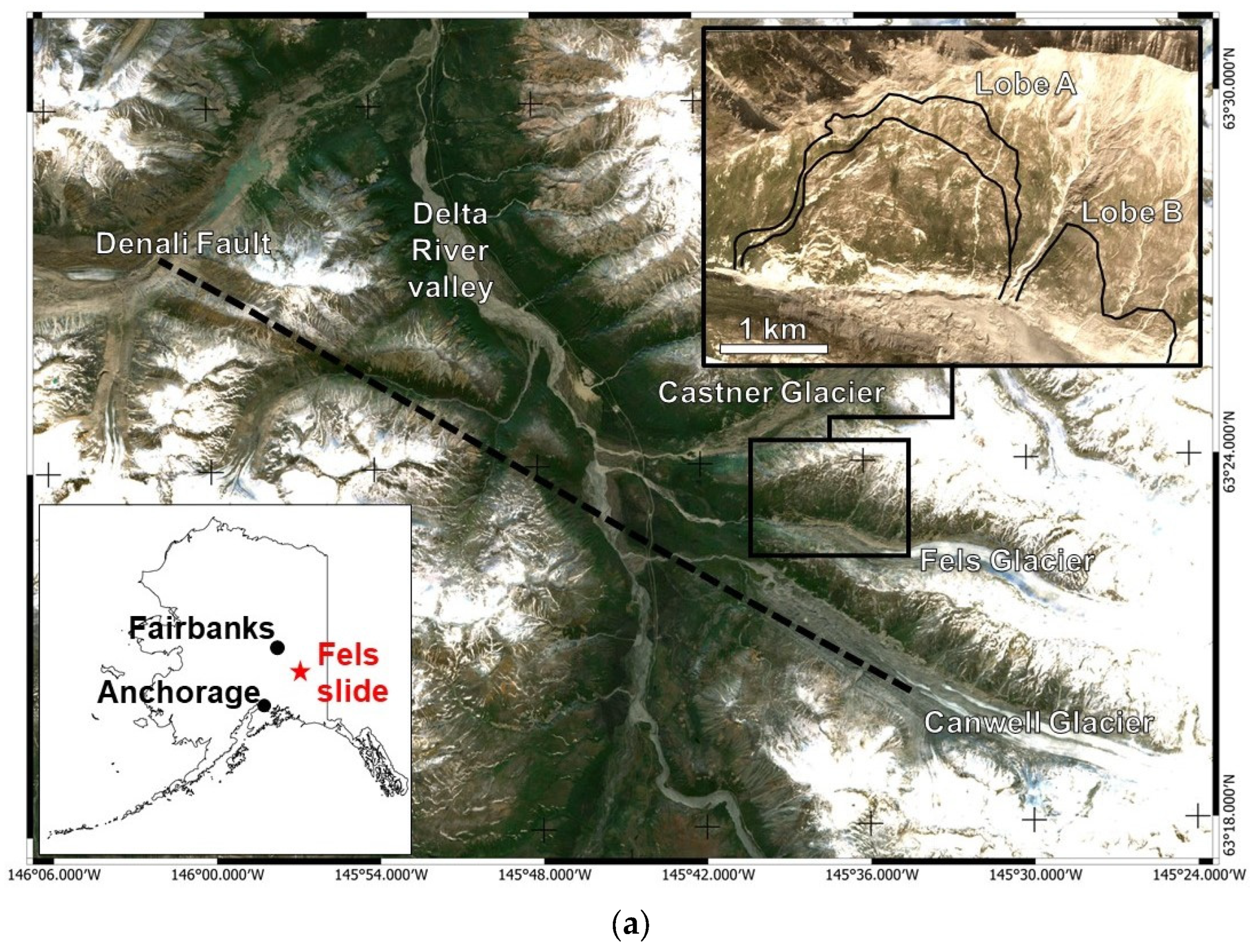
The Fels landslide is located within the Alaska Range, 150 km southeast of Fairbanks, Alaska. The landslide lies on the north slope of the Fels Glacier valley, an E-W-trending tributary of the Delta River valley (Figure 1a), and was first identified in 2013 [32]. The Richardson Highway, which connects Fairbanks to the coastal town of Valdez, and the Trans-Alaska Pipeline, which extends from oil fields on the north shore of Alaska to the Valdez Marine Terminal, pass through the Delta River valley.
Two adjacent and distinct areas of active slope deformation, separated by a prominent gully, referred to as “Lobe A” and “Lobe B”, exist within the Fels Glacier valley (Figure 1a; [32]. The Fels landslide corresponds with the area of Lobe A, which, compared to Lobe B, is characterized by significantly higher deformation rates. Lobe A also displays a spatially varied distribution of displacement rates. The western part of the lower slope displays evidence of active instability, mainly in the form of steep scarps, and is hereafter referred to as “fast-moving toe” (Figure 1b). The central part of the landslide has spatially homogeneous displacement rates. In comparison, the upper part displays an abrupt decrease in displacement rates (upper right inset in Figure 1a). The north slope of the Fels Glacier valley dips about 20–30° SSW, increasing to 40–50° near the Fels Glacier. The landslide has an area of 2.3 km2 and extends down to the toe of the glacier, about 3 km above the mouth of the Fels Glacier valley. It has a measured length of 1400 m in the E-W direction and 1600 m in the N-S direction (between elevations of 920 and 1490 m above sea level (a.s.l.)).
Bedrock on the north slope of the Fels Glacier valley comprises fine-grained Devonian metasedimentary rocks of the Jarvis Creek Glacier subterrane, primarily quartz-mica schist and quartzite, and secondly chlorite-muscovite schist, calc-schist, marble, and basalt [34,35]. Within the landslide area, bedrock is blanketed by colluvium, which is involved in local surficial rotational sliding, especially on the lower part of the slope. Bedrock crops out locally within deeply incised gullies and in sub-vertical geomorphic steps at higher elevations. The bedrock is characterized by a prominent undulatory foliation that dips between 20 and 25° SSW within the landslide area. The foliation is sub-parallel to the slope and possibly controls its morphology, as noted by Newman (2013). On a larger scale, the foliation dips more steeply to the south, reaching up to 50–60° near the Denali Fault [35].
The Denali Fault is an active, right-lateral strike-slip fault that follows the Canwell Glacier valley south of the Fels Glacier valley (Figure 1a). An MW 7.9 earthquake occurred on this fault on 3 November 2002, accompanied by up to 5.3 m of right-lateral slip, as estimated within nearby Delta River valley [36,37], and hundreds of rock avalanches, rockslides, rotational slides, and debris avalanches within the epicentral area [38,39]. The area of the landslide was also affected by ground shaking during the 1964 MW 9.2 Good Friday earthquake, which had a source beneath Prince Williams Sound about 320 km to the WSW. In this case, the ground motions were considerably attenuated over a large distance from the earthquake source [40].

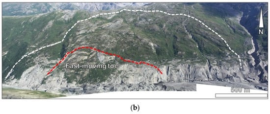
Figure 1.
Overview of the Fels landslide. (a) Satellite view of the intersection of the Delta River and Castner, Fels, and Canwell valleys (Copernicus–Sentinel 2 imagery). The black dashed line marks the trace of the Denali Fault. The insets show the location of the Fels landslide in Alaska and a satellite view of the landslide area [41]. Black curved lines in the upper right inset delineate the areas of “Lobe A” (i.e., the Fels landslide) and “Lobe B” where deformation has also been detected. The upper part of Lobe A, characterized by significantly lower deformation rates, is also outlined. (b) Frontal view of the landslide from the crest of the ridge on the south side of Fels Glacier valley. The white dashed line marks the boundary of the inferred unstable area, and the red dotted line delineates the upslope boundary of its fast-moving toe. Note the absence of a well-defined landslide headscarp.
A full understanding of the Fels landslide requires knowledge of the evolution of the Fels Glacier valley. The valley, in some form, has existed since the Pliocene, possibly since the Miocene, but it was profoundly deepened and widened by glaciers during the Quaternary Period. Repeated glaciations steepened the valley walls and increased the local relief. Glacier flow has exacerbated rock slope instability by damaging the rock mass [42]. During periods of glacier retreat, the removal of lateral slope support provided by the glacier ice further reduced the kinematic constraint of the rock slope [43,44,45]. During the last Pleistocene glaciation, the Cordilleran Ice Sheet extended over the Alaska Range, burying Fels valley beneath up to 1.4–1.5 km of glacier ice [46]. By about 11,000 years ago, the ice sheet had disappeared, but an alpine glacier (Fels Glacier) has remained in the valley ever since. The Fels Glacier achieved its maximum Holocene extent during the Little Ice Age when it extended into Delta River valley and constructed the prominent lateral and end moraines there [35]. At the peak of the Little Ice Age, the surface of the Fels Glacier opposite the fast-moving toe of the Fels landslide had an elevation of about 1115 m a.s.l., about 115–140 m above the present glacier surface. In this paper, the progressive thinning and retreat of the Fels Glacier are investigated to highlight the potential correlation between ongoing climate change and the stability and geomorphic evolution of the slope.
3. Materials and Methods
3.1. Workflow
The present research builds on a study by [32], who presented a slope characterization of the landslide based on a combination of traditional geological and geomechanical mapping. Refs. [32,47] presented preliminary ALS and DInSAR results for motion of the landslide. Our research significantly expands the scope and findings described in these works by combining advanced multi-temporal and multi-sensor remote sensing datasets to provide an improved interpretation of the failure mechanism and to highlight the evolution of the landslide behavior over the past 60 years.
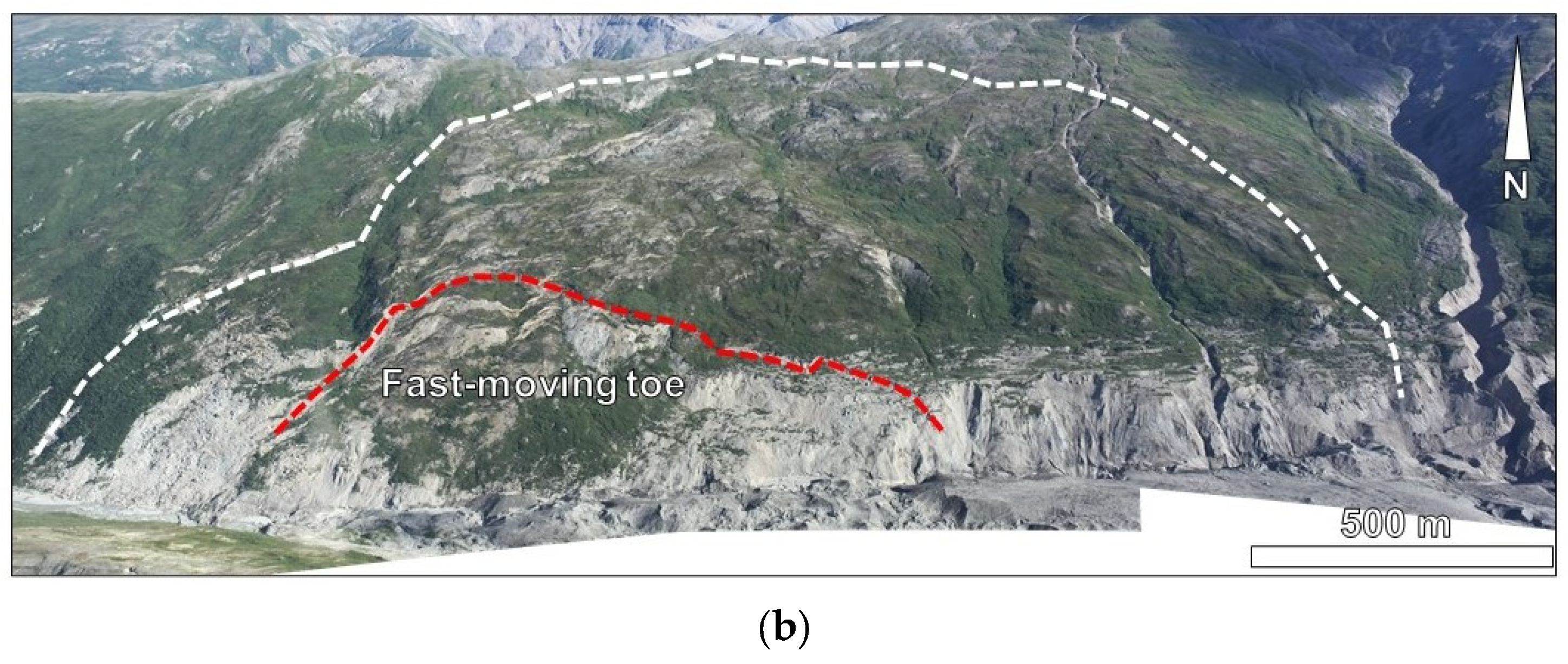
This research follows the workflow summarized in Figure 2. The workflow comprises five stages: field characterization, historical analysis, multi-scale (i.e., slope and rock mass) characterization, SAR data processing, and an integrated interpretation. Alyeska Pipeline Service Company provided ALS for 2014 and 2016 and access to the site for ground-based field and remote sensing characterization. Table 1 provides a summary of the remote sensing datasets used in this research, together with relative information on the source, scale, and resolution.
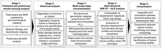
Figure 2.
Research flowchart. Detailed results from Stage 1 are described in [32].

Table 1.
Summary of remote sensing datasets used in this research, ordered by type and scale. For each dataset, source and resolution are reported.
3.2. Stage 1: Field Characterization
Field work was undertaken in 2010 to characterize the Fels landslide from a geological and geomechanical perspective. The location, extent, and orientation of geomorphic features, such as uphill- and downhill-facing scarps, tension cracks, benches and steps, and slope bulging, which are indicative of deep-seated slope deformation, were recorded. Field observations also included geological, structural, and geomechanical data, such as lithology, foliation planes, fold axes, fracture orientation, spacing, persistence, infilling and surface conditions, intact rock strength values [48], and geological strength index [49]. At three stations, intact rock and discontinuity data were systematically recorded using a scanline mapping approach [50]. A detailed description of the field characterization program conducted is beyond the scope of this paper; the interested reader is referred to [32] for details. In this paper, selected extracts of Newman’s work that are relevant to the described remote sensing analyses are presented.
3.3. Stage 2: Historical Analysis
A visual analysis of Fels valley was performed using historical air photographs (August 1949, June 1977, August 1981; resolution about 1 m/pixel), satellite imagery (August 2010; RapidEye image; 5 m/pixel), and an orthophoto obtained during a helicopter survey (August 2017; 0.5 m/pixel). Both historical air photographs and satellite imagery were obtained from the USGS “Earth Explorer” database (https://earthexplorer.usgs.gov/, accessed on 1 October 2023). The available databases were filtered using a polygon with the extent of the investigated area. The 2017 orthophoto was created using an SfM approach, using photographs collected at multiple stations on the opposite side of the valley and during a helicopter survey (see Section 3.4). This analysis enabled an investigation and quantification of both the progressive development of surface cracking through time and retreat of Fels Glacier from the lower part of the valley. Each image was registered in ArcMap 10.6 [51] using the coordinates of natural points obtained from the ALS dataset available for the study. These points are located outside the landslide area and are considered to be stable through time. Surface cracks visible on the air photographs were then digitized as polylines, following the workflow described by [8]. The total length of all polylines was computed for each analyzed air photograph. Based on the distribution of lineaments identified in the historical imagery, the area of the fast-moving toe of the landslide was outlined and computed. The outline of Fels Glacier was manually digitized in each air photograph, and its terminus was identified and mapped. The glacier retreat was estimated by measuring the distance of the terminus along the valley axis in each image from its position in the first (1949) photograph. Finally, the surface elevation of glacier ice was estimated by sampling points on the 2016 ALS dataset at the slope/glacier interface in the mid-point location of the fast-moving toe area.
3.4. Stage 3: Multi-Scale Slope Characterization
The third stage of the investigation is an engineering geomorphic characterization of the slope using remote sensing techniques. The analysis was undertaken at progressively larger scales. First, a slope-scale landslide characterization was undertaken in ArcMap. Hillshade, aspect, and slope maps derived from the 2016, 1 m resolution ALS dataset were created using built-in tools in ArcMap. These thematic maps were employed to identify and map linear geomorphic features such as scarps, antislope scarps, tension cracks, and gullies [6,52]. The geometric characteristics of these elements, for example, trend and length, are commonly controlled by faults and joints, which represent weak planes within the rock mass that are exploited by weathering, erosion, and deformation processes [53]. Consequently, linear geomorphic features can be considered proxies that potentially record the style of deformation of the slope and its geomorphic evolution.
The trends (i.e., the azimuth) of all the mapped lineaments were reported in a summary table, which was then imported into the software DIPS 8 [54] for interpretation. Rosette diagrams were used to identify and visualize the principal trends of geological structures within the slope, which in other studies have been shown to coincide with the orientations of major geomorphic elements such as valleys, gullies, ridges, and landslide boundaries [45,55]. These results were compared with preliminary lineament mapping described by [32], which was completed using a lower resolution digital elevation model (1/3 arc-second, about 10 m), as well as optical satellite imagery and a LiDAR DEM with partial coverage of the landslide.
At a larger scale, a Riegl VZ-4000 laser scanner with a maximum operating range of about 4 km was used to perform a TLS scan of the unstable Fels valley slope in the summer of 2017 from a location 700–2000 m away on the opposite side of the valley. High-resolution photographs were obtained using a 50 MPixel Canon EOS 5Ds-R digital reflex camera mounted on a Gigapan robotic tripod head and coupled with a f = 200 mm focal length lens. Geotagged photographs were taken from four camera stations on the south side of Fels valley and used for the SfM reconstruction of the slope in combination with photographs acquired during a helicopter survey. In addition to the 3D SfM model, the photogrammetric survey provided an updated orthophoto of the area, including the terminus of Fels Glacier. An infrared thermography (IRT) analysis was performed with a FLIR SC7750 thermal camera, coupled with a f = 50 mm focal length lens, to investigate seepage from the unstable slope. The analysis of the IRT dataset was conducted using the software ResearchIR 4 [56].
The previous study by [32] and the multi-stage slope characterization of this study allowed for the identification of locations on the colluvium-blanketed slope where bedrock is exposed, and thus, remote sensing engineering discontinuity mapping could be effectively undertaken. Outcrop-scale remote sensing mapping was conducted along a deeply incised gully that marks the eastern boundary of the landslide area. The gully wall could not be safely accessed; therefore, a close-range SfM approach was used to build an oriented 3D model of the outcrop (i.e., a virtual outcrop). To do so, high-resolution, geotagged photographs of the outcrop were collected from distances ranging from 5 to 15 m at more than 10 stations along the opposite side of the gully. Discontinuity data were then extracted from the 3D model using the software CloudCompare 2.12 [57]. The orientations (i.e., dip and dip direction) of the mapped discontinuities were plotted in a stereonet using DIPS, and the major discontinuity sets, including foliation, within the rock mass were identified.
3.5. Stage 4: Multi-Temporal ALS and SAR ST Analysis
Next, a change detection analysis using the 2014 and 2016 ALS datasets (both with 1 m resolution) was performed. The change detection analysis was conducted by subtracting, pixel-by-pixel, the elevation in 2016 from that in 2014, thus providing the vertical deformation over an equal-sized raster grid.
An advanced ST analysis was then performed, following the workflow outlined in [31], using RADARSAT-2 spotlight mode imagery. Ref. [31] also provides a detailed description of the SAR-ST method applied to landslide analyses, as well as specifications with regard to detail, advantages, limitations, and applicability. The analysis focused on two consecutive five-year time windows, namely 2010–2015 and 2015–2020. For each time window, the ST analysis provided the cumulative surface displacement along the three principal components (E-W, N-S, and vertical) of the displacement vector. ST data were then post-processed in ArcMap, where raster datasets and thematic maps of the magnitude, azimuth, and plunge of the surface deformation were created. By comparing, pixel-by-pixel, the difference between the 2010–2015 and 2015–2020 time windows, it was possible to recognize and quantify the changes in the style of deformation and failure mechanism that occurred over the 10-year period covered by the ST investigation. A qualitative comparison of the deformation maps computed from the ST datasets was performed, and the lineament map developed in the previous stage of this study was examined to identify the geological structures that control slope deformation.
Next, profiles of slope elevation, deformation magnitude, and displacement plunge along the slope were created to infer the state of activity of the landslide and its differences in space (i.e., across the landslide area) and time (i.e., 2010–2015 vs. 2015–2020). Finally, the morphology of the failure surface of the landslide was reconstructed using the vector inclination method (VIM; [58]).
3.6. Stage 5: Integrated Interpretation
In the final stage of the study, the results obtained from the preceding four stages were integrated and analyzed. An interpretation of the landslide, its classification according to the scheme of [33], and an analysis of the factors that controlled the evolution of the landslide are provided.
4. Results
4.1. Historical Analysis
The analysis of historical air photographs and satellite imagery revealed a significant increase in the cumulative length of surface cracks over time (Table 1). Surface cracks were visible near the toe of the slope in the 1949 air photograph, indicating that the landslide has been active since before 1949 (Figure 3a). Between 1949 and 1977, cumulative surface cracking in the landslide area increased from about 1300 m to 2100 m, from which an average increase of surface cracking length of 75 m/year was derived. The cumulative length of the surface cracking increased to 3550 m by 1981, 9750 m by 2010, and 12,760 m by 2017 (Figure 3a,b), corresponding to increases in surface crack length of 890 m/year, 340 m/year, and 1800 m/year for the time windows 1977–1981, 1981–2010, and 2010–2017, respectively (Figure 3b).
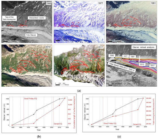
Figure 3.
Summary of historical analysis of Fels Glacier and the deforming slope bordering its toe. (a) Progressive growth of surface slope damage features (solid red lines) mapped on historical air photographs. The tab in the lower left corner provides a summary of the progressive retreat of the toe of Fels Glacier based on historical air photographs. The elevation of the slope–ice interface was sampled at the location of the white line. (b,c) Plots showing changes in, respectively, cumulative crack length and surface area of the fast-moving landslide toe and glacier ice surface elevation over time.
Based on the analysis of aerial and satellite imagery, the Fels Glacier retreated over 1000 m over the 68-year period 1949–2017 (Table 1). Over that time, the total lowering of the glacier surface at the center of the fast-moving toe of the Fels landslide was 79 m. Between 1949 and 1977 and between 1981 and 2010, the glacier retreated approximately 410 m and 430 m, respectively, from which an average rate of retreat of 15 m/year was derived (Figure 3a). Between 1977 and 1981, the glacier retreated about 157 m, yielding an average retreat rate of 39 m/year. The differences in the computed retreat rates may be biased by the different months in which the images were captured (i.e., June in 1977 and August in 1981). Disregarding the 1977 data point, the total retreat between 1949 and 1981 is 567 m, from which an average rate of retreat of 18 m/year was calculated. Notably, between the 1960s and early 1980s, glaciers around the world, including Alaska, stabilized and advanced short distances (e.g., [59,60,61]). It is likely that the Fels Glacier stabilized and advanced during the same period; thus, the average rates for the periods of 1949–1977 and 1977–1981 are biased by this variability. It is estimated that the glacier retreated an additional 30 m between 2010 and 2017 (average rate = 4 m/year).
The area of the fast-moving toe of the Fels landslide progressively increased over time (Table 2). In 1949, the surface area of the fast-moving toe was about 200,000 m2. It increased to about 235,000 m2 in 1977, 236,000 m2 in 1981, 266,000 m2 in 2010, and 320,000 m2 in 2017 (Figure 3c).
Table 2.
Evolution of Fels Glacier and Fels landslide from 1949 to 2017.
4.2. Multi-Scale Slope Characterization
4.2.1. Slope-Scale Analysis
The entire landslide area is characterized by vegetation-free failure scarps that highlight the ongoing instability affecting the slope (Figure 4). Particularly prominent rotational slide scars, with dip angles up to 50° and heights up to 50 m, characterize the fast-moving toe and mark its lateral and rear boundaries (I in Figure 4). No bedrock daylights are seen within these prominent features, suggesting that the minimum thickness of the blanketing colluvial deposit on the lower slope is 50 m. Above the fast-moving toe, rotational slides appear to be more superficial, with elevations and lengths that progressively decrease toward the upper slope.
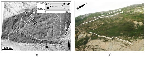
Figure 4.
Overview of the Fels Glacier valley slope. (a) Hillshade map derived from the ALS dataset. Profile A-A’, plotted in the inset, extends across the northwest boundary of the landslide area and intersect the geomorphic steps discussed in the text. (b) Photograph (view to the northwest) taken from a helicopter. Line I is the upper limit of the rotational sliding instability of the fast-moving toe. Lines II and III mark scarps at the northwest boundary of the landslide. Line IV delineates a gully that marks the east boundary of the landslide.
Persistent linear features (i.e., length > 500 m) on the failing slope reflect a significant structural control on their location and orientation. A NE-SW-oriented, sub-vertical scarp with a length of about 800 m and a height of about 10 m crosses the slope between 1240 and 1400 m a.s.l. (II in Figure 4). Just west of this feature is another structurally controlled geomorphic step (III in Figure 4) with a similar orientation and length but a significantly lower dip angle, possibly due to erosion at the crest and deposition at the base of the slope. It likely is older than the sub-vertical scarp, below which a two- to three-fold increase in deformation rates in the SAR ST dataset is observed (see Section 4.3). The trend of these features is similar to that of the prominent gully on the east side of the landslide (IV in Figure 4), suggesting that the gully’s location may also be controlled by bedrock discontinuities. The Fels Glacier flows in an ESE-WNW direction past the landslide area. However, to the east, outside the landslide area but near the gully, the glacier flows in a SE-NW direction, about 20° different from the downvalley flow direction. This change in the orientation of the valley axis is likely controlled by geological structure (Figure 5a).
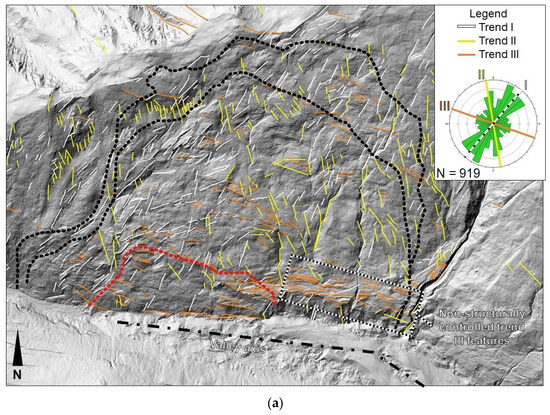
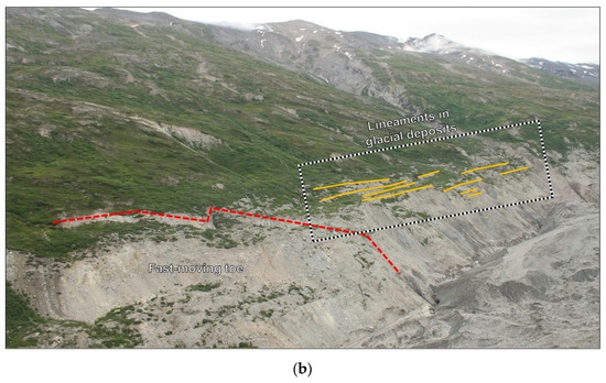
Figure 5.
Results of lineament analysis. (a) Lineament map showing the mapped features, which are color-coded based on orientation. The dotted black lines delineate the approximate upslope boundary of the landslide and, below it, the internal boundary, below which higher displacement rates are observed. The red dashed line marks the boundary of the fast-moving toe. Trend III lineaments on the east part of the lower slope are likely controlled by surface deformation of Little Ice Age glacial deposits. The change in orientation of the valley axis is also highlighted by the dash-dotted black line. (b) Oblique view of the trend III lineaments in glacial deposits on the lower slope, which are independent of geological structures.
Lineaments were placed on the GIS thematic maps to further highlight the potential correlation between geomorphic features and structural geology. Rosette diagrams illustrating the mapped lineament orientations define three major trends (Figure 5a), which are referred to as trends I, II, and III based on the relative number of lineaments mapped. Trend I includes lineaments with a SW-NE orientation, parallel to the geomorphic steps (II and III in Figure 4) and the gully that marks the east boundary of the landslide (IV in Figure 4). Trend II comprises lineaments oriented in an NNW-SSE direction parallel to the east landslide boundary. Trend III comprises lineaments with an ENE-WSW orientation, which is sub-parallel to the orientation of the Denali Fault and the rear boundary of the landslide area. The orientation of the valley axis east of the gully also correlates with trend III and aligns with the rear boundary of the wedge-shaped, fast-moving toe, further supporting the control exerted by the geological structure on the evolution of the valley and landslide (Figure 5a). However, on the east part of the lower slope, features similar in orientation to trend III occur in glacial deposits. Lineaments in this area represent lateral moraines rather than geological structures. Similar results were reported by [32], who identified three prominent lineament trends oriented NNE-SSW, NE-SW, and E-W, in good agreement with trends I, II, and III of our study.
Infrared photographs obtained from the slope opposite the Fels landslide were stitched into a single panoramic image (Figure 6. Groundwater seepage is concentrated on the lower slope, particularly within the colluvial deposit near the valley bottom (Figure 6). It seems likely that the south-dipping foliation exerts some control on groundwater flow. Surface runoff from rainfall and snowmelt is concentrated along gullies within the slide area (Figure 6). Significant snow patches were still visible at the higher elevations when the infrared survey was performed in August 2017.

Figure 6.
IRT dataset showing differences in surface temperature that can be correlated with vegetation (or absence thereof), groundwater seepage, and snow patches. Dotted white and red lines mark the boundary of the landslide area and the fast-moving toe, respectively.
4.2.2. Outcrop-Scale Analysis
The bedrock outcrop that was surveyed is located at an elevation of about 1450 m a.s.l. on the east wall of the gully on the east side of the slide area (Figure 4a). The orientation and persistence of the discontinuities obtained by processing the point cloud in CloudCompare are plotted in the stereonet shown in Figure 7. The rock mass discontinuities can be placed into three main sets that are sub-perpendicular to each other and are referred to as D1, D2, and D3. D1 discontinuities are foliation planes. They are characterized by an average mapped persistence of 8 m and an orientation of 36°/228° (hereafter, all orientations are expressed using a dip/dip direction convention), sub-parallel to the slope surface. D2 discontinuities have an average persistence of 5.7 m and are characterized by a sub-vertical orientation of 87°/135°, sub-parallel to the gully and the outcrop surface. D3 discontinuities, with an average persistence of 4 m, dip into the slope with an orientation of 44°/19°, sub-perpendicular to the slope surface. However, the orientation of this discontinuity set, combined with the low height of the outcrop (6–7 m), results in censoring [62] that is difficult to estimate and correct.
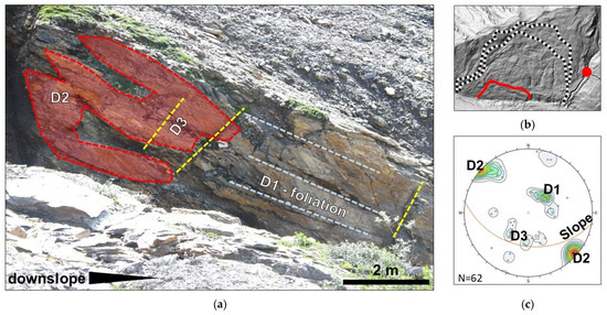
Figure 7.
Outcrop-scale analysis. (a) Close-up view of the investigated outcrop, highlighting the discontinuity sets identified during discontinuity mapping. Note the slope-parallel bedrock foliation (D1); discontinuity set D2, which is sub-parallel to the outcrop; and discontinuity set D3, which is sub-perpendicular to both D1 and D2. (b) Hillshade map of the slope showing the location of the investigated outcrop (red dot), which is outside the slide area. Black and white line mark the boundary of the landslide. Red line marks the boundary of the fast-moving toe. (c) Stereonet (lower hemisphere, equal angle) showing the results of the discontinuity mapping.
The results from the remote sensing outcrop-scale analysis display some agreement with field data reported by [32], including an average foliation orientation of 27°/207° and a sub-vertical northwest-dipping set (referred to as J1) that correlates with D2 in this study. Reference [32] also reported two minor sub-vertical north- and northeast-dipping discontinuity sets in the west part of the landslide area; however, we did not observe them in the investigated outcrop. The observed differences are likely due to the greater number of localities investigated by [32], both within and outside the landslide area. In this study, only rock outcrops outside the slide area were investigated.
4.2.3. Comparison of Slope- and Outcrop-Scale Datasets
A similarity between the outcrop-scale discontinuity data and orientations of slope-scale lineaments was noted after plotting the rosette diagrams. Specifically, correspondence was observed between lineament trend I and discontinuity set D2 and between lineament trend III and discontinuity set D3 (Figure 8a). D1 discontinuities (i.e., bedrock foliation) are unlikely to control surface lineaments due to their slope-parallel orientation. Lineament trend II does not display any obvious correlation with the outcrop-scale discontinuity sets. The correlation between rock mass discontinuities and surface lineaments suggests the latter are primarily controlled by geological structures. In turn, the distribution of surface movements is controlled, to a certain extent, by deformation that occurs at depth within the slope below the colluvial blanket. An example is the fast-moving toe (Figure 8b). The geomorphic processes and features that can be observed within this area, such as the retrogressive behavior and high scarps, are typical of roto-translational or pseudo-rotational failures that occur in soil and weak rock slopes. However, the boundaries of this large, unstable area are clearly aligned with both the interpreted lineaments and the outcrop-scale discontinuities, suggesting that geological structures play an important role in defining the dimension and shape of the fast-moving toe.

Figure 8.
(a) Rosette diagrams showing slope-scale lineaments and the outcrop-scale discontinuities. (b) Potential correlation between the discontinuity sets identified during the outcrop-scale analysis (D2-D3) and the lineaments (I-III) delineating the boundaries of the landslide (dotted black line, excluding the low displacement rate area) and the fast-moving toe (red dotted line).
4.3. Multi-Temporal ALS and SAR ST Analysis
4.3.1. ALS Change Detection
The ALS datasets collected in 2014 and 2016 were compared to identify areas within the investigated slope with vertical deformation over the two-year period (Figure 9a). Significant downward displacements occurred within the fast-moving toe over this period. It was noted that elevation changes progressively increased in magnitude from the west boundary of the landslide (<4 m) to the east part of the fast-moving toe (4–6 m). The raster dataset produced from the change detection analysis displays fringes across the fast-moving toe, with an alternation of stripes with positive and negative vertical displacements. Such a pattern suggests that the fast-moving toe is progressively moving toward the valley bottom while breaking-up in a series of rotational slides. The stripes with different vertical displacements are parallel to lineament trend III, supporting the hypothesis of strong structural control on the evolution and behavior of the fast-moving toe. An area with an elevation gain of up to 1.1 m is located just upslope of the fast-moving toe and exhibits a forward movement (i.e., out of the slope) rather than an actual upward displacement. This interpretation is supported by the generalized elevation loss (up to 50 cm) that we observed across the upper part of the main landslide body, which is the area where most of the elevation changes and total displacement are recorded (Figure 9b).
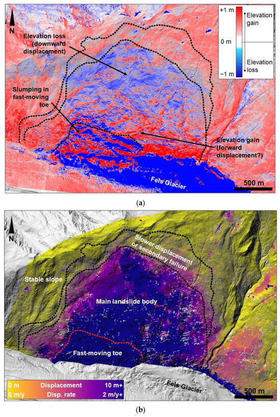
Figure 9.
(a) The 2014–2016 ALS change detection results and (b) total 2010–2020 displacements derived from the ST analysis. Note the significant elevation changes on the lower slope, the elevation gain on the central part of the slope (shades of red, possibly related to a forward, out-of-the-slope displacement), and the elevation loss on the upper slope (shades of blue). The dotted lines mark the boundaries between the fast-moving toe, the main landslide body, the slower displacement (possible secondary failure) area, and the stable part of the slope. In the slower displacement area, observed displacements are greater than the measurement error, but displacement magnitudes and elevation changes are significantly smaller than in the main landslide body.
4.3.2. Characterizing Landslide Displacement Using the Speckle-tracking Datasets
The ST analysis was conducted using SAR images obtained over two subsequent five-year time windows: 2010–2015 and 2015–2020. The displacement magnitude maps for each period (Figure 10a,b) show surface movements of more than 10 m on the fast-moving toe. Over the combined ten-year period, the fast-moving toe locally moved up to 75 m. The wedge shape of the fast-moving toe is clear in both maps. Above the fast-moving toe, the total displacement progressively decreases toward the upper slope. Near the upper boundary of the landslide, the total displacement over the 2010–2015 and 2015–2020 time windows is about 30–60 cm. The achievable accuracy of ST techniques is typically between 1/10th and 1/100th of the spatial resolution of the SAR image dimension (5 × 1.5 m in this case) [63]. Therefore, we consider displacement values lower than 50 cm to be background values for the purpose of this analysis.

Figure 10.
Maps of computed total displacements and displacement rates for the (a) 2010–2015 and (b) 2015–2020 time windows. The yellow and the white dotted lines outline the fast-moving toe and the boundary of the landslide area, respectively. The black dotted lines in (a,b) outline the areas with the largest displacements. Lines II and III mark the geomorphic features shown in Figure 4. Note the increase in displacements between the 2010–2015 and 2015–2020 time windows and the upward propagation of the fast-moving toe highlighted in the 2015–2020 displacement map.
The 2010–2020 displacement magnitude maps highlight the differences in displacement rates across the landslide area (Figure 9b). The limits of resolutions of displacement values (i.e., the computed displacement in the parts of the slope that are considered to be stable), which is 100 cm over the 2010–2020 survey period, were used to identify and trace the landslide boundaries. Areas where the computed displacements exceeded this threshold are considered to be part of the landslide. To the west, displacements are greater than 5–6 m below the 10 m high scarp (II in Figure 10) and significantly decrease above the scarp. Upslope of the 30 m high geomorphic step (III in Figure 10), displacements progressively decrease to background values. This 30 m high scarp roughly divides the main landslide body, where most displacement and elevation changes occur, from the area where instability progresses more slowly. To the east, displacements decrease significantly near the gully where the outcrop-scale survey was performed (IV in Figure 10). There, deformation may be partly affected by surface erosion or by slumping into the gully itself. To the north, in the area where the ALS change detection analysis showed a predominant elevation loss (Figure 9), displacements reached 10 m between 2010 and 2020. Upslope, displacements up to 4–5 m are observed within the slowly moving area of the landslide. Similar displacement magnitudes are also observed to the northeast, but their trend to the SSE (Figure 11a) suggests that they are generated by surface movements toward the gully (e.g., slumping or erosion) and are, therefore, not part of the Fels landslide. East of the gully, within the area referred to as Lobe B (Figure 1a), we observed some displacements (up to 5.5 m) up to an elevation of 1350 m a.s.l. on the lower slope. The absence of obvious, structurally controlled deformation features in this area does not allow the depth of the movement to be confidently inferred. In general, a significant increase (up to 30%) is apparent in total displacement magnitudes across the central and upper parts of the unstable slope between the 2010–2015 and 2015–2020 time windows (Figure 10a,b). Conversely, on the fast-moving toe, total displacements generally decreased (as much as 20 m in places) between the two time windows, although there are local areas of increased displacements. For example, there is a significant increase in displacement magnitude along the northeast boundary of the fast-moving toe, with a difference in displacement magnitudes >10 m between the two time windows. An increase near the northwest boundary was also noted, indicating a generalized upslope propagation of the fast-moving toe (Figure 10b).

Figure 11.
Maps of trends and plunges of displacements based on the 2015–2020 time window. (a) Displacement trends. Note the overall SSW displacement of the landslide. (b) Displacement plunges. Note the changes in plunge over the upper, central, and lower parts of the slope. The fast-moving toe, entire landslide area, and the portion of the landslide area where significant displacements occur are outlined in (a,b).
The displacement trend map shows a near-constant SSE (175°–195°) direction of movement over the entire landslide area, with only minor spatial variations likely due to surficial deformation (Figure 11a). The most significant spatial variations of the movement direction within the fast-moving toe, where displacement trends range between 100° and 230°, are roughly perpendicular to lineament trends I and III, respectively. However, the average trend of movement direction here is in accord with that on the rest of the unstable slope. Conversely, the northwest sector of the landslide area and the east part of the upper slope display a southeast displacement trend (about 100–110° and 140–150°, respectively).
A map of displacement plunge provides information useful for the interpretation of slope deformation (Figure 11b). The fast-moving toe is characterized by displacement plunge values up to 50°. The occurrence of such a strong vertical downward component of deformation agrees with field observations and the progressive breaking-up of the lower slope through a series of roto-translational and pseudo-rotational failures. Behind the fast-moving toe, computed displacement plunge values decrease to 20–22°, with only local increases that are possibly due to surface rotational sliding. At elevations between 1360 m (to the west) and 1160 m (to the east), displacement plunge angles increase to 36°, although there is considerable variability with values as low as 20°. Such variability is also interpreted as resulting from local surface rotational sliding. Consistently high displacement plunge values (up to 50°) are also evident near the northwest boundary of the slide area within the slow displacement area (Figure 9b), possibly related to secondary instability (i.e., slope failures driven by the displacement of the main landslide body).
4.3.3. Profile Construction and Description
Profiles from the GIS maps allow changes in displacement magnitude and plunge between the 2010–2015 and 2015–2020 time windows to be quantified and compared with the topography of the slope (Figure 12). Longitudinal profiles reveal the magnitude of the computed temporal (2010–2015 vs. 2015–2020) change down the slope, with positive and negative changes indicating, respectively, an increase or a decrease in displacement magnitude derived from the ST analyses. Displacement plunge data can also be plotted along longitudinal profiles to highlight details of the deformation mechanism and the morphology of the failure surface, assuming that the trend along the profile is controlled by the orientation of the failure surface. In general, higher positive or negative values indicate, respectively, steeper downward or upward displacement vectors and, in turn, a steeper failure surface. The horizontal parts of longitudinal profiles correspond to areas with a uniform displacement plunge, which likely indicates translational movements along a surface with a constant dip angle (i.e., planar sliding). Conversely, an upward or downward concavity of the displacement plunge profile indicates, respectively, a decrease or increase in the downward component of the displacement vector. Expressed differently, an upward concavity in the displacement plunge profile corresponds to a downward concavity in the failure surface, and vice versa.
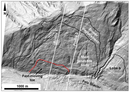
Figure 12.
Locations of profiles 1 and 2. The boundaries of the entire landslide, the fast-moving toe, and the part of the landslide where the greatest displacements occur are shown.
Two longitudinal profiles were constructed down the steepest portion of the slope and parallel to the dip of the rock foliation (Figure 12). Both profiles extend across the entire body of the landslide, including the fast-moving toe. Analysis of profile 1 shows the increase in slope deformation in the 2015–2020 time window relative to the 2010–2015 period (Figure 13a). The increase in displacement begins near the upper boundary of the landslide, which, in this case, does not correlate with any obvious geomorphic feature and is maintained across the entire profile.
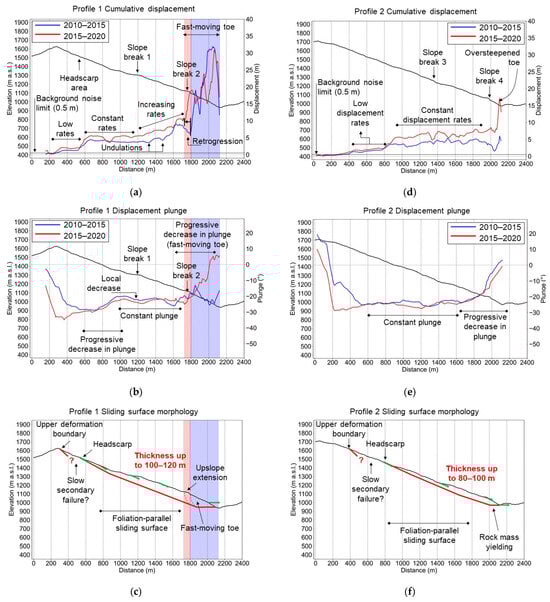
Figure 13.
Summary of profile analysis and VIM failure surface reconstruction. (a) Cumulative displacement (2010–2015 and 2015–2020) along profile 1. (b) Displacement plunge (2010–2015 and 2015–2020) along profile 1. (c) Failure surface reconstruction along profile 1 based on plunge and displacement data. (d) Cumulative displacement (2010–2015 and 2015–2020) along profile 2. (e) Displacement plunge (2010–2015 and 2015–2020) along profile 2. (f) Failure surface reconstruction along profile 2 based on plunge and displacement data. Blue and red zones in the plots indicate, respectively, the extent of the fast-moving toe in the 2010–2015 ST dataset and the upslope extension noted in the 2015–2020 dataset.
Displacements start along profile 1 near the crest of the slope at an elevation of 1600 m a.s.l. However, rates are low (about 25 cm/y) down to 1500 m a.s.l., where displacements are in excess of 5 m (1 m/y) for both the 2010–2015 and 2015–2020 time windows. At about 1300 m a.s.l., there is a change in slope angle at the surface (slope break 1 in Figure 13a) and the displacement magnitude progressively increases downward toward the toe of the slope. A spike in displacement at 1120 m a.s.l. corresponds to the upper limit of the fast-moving toe, a prominent slope break (slope break 2 in Figure 13), and an increase in the slope angle. This abrupt increase in displacement starts about 50 m farther up the slope in 2015–2020 than in 2010–2015, indicating that the area of fast deformation propagated upslope by this amount over the ten-year period (Figure 13a). The total displacement along profile 1 displays, along its entire length, some undulations, which cause deformation to locally decrease downslope (Figure 13a,d). These undulations probably result from the overlapping effects of slope deformation at depth and local surface rotational sliding. In this interpretation, the maximum magnitude of slumping-related displacements correlates with the peaks of the undulations, whereas areas with limited or no surface rotational sliding correlate with negative peaks in displacement magnitude. Displacement plunge values near the slope crest display significant differences between datasets. However, considering the low magnitude of the displacements in that area, these are likely related to data noise. Between 1600 and 1480 m a.s.l., displacement plunge values are approximately 30° in both time windows. Between 1450 and 1380 m a.s.l., displacement plunge progressively decreases from 30° to about 22°. In the central part of the slope, the displacement plunge angle is approximately constant at 20–22°. On the lower slope, near slope break 2, the displacement plunge sharply decreases (i.e., the profile curve moves upwards), albeit with significant superposed spatial undulations. This decrease in displacement plunge is particularly evident in the 2015–2020 time window. Displacement magnitude and topography display a good correlation along longitudinal profile 1. Each slope break correlates with a change in the displacement rate downslope. A significant change in both displacement plunge and displacement magnitude correlates with slope break 2 located at 1100 m a.s.l. (Figure 13). Slope break 1 at 1300 m a.s.l. seems to correlate with a minor, negative peak in the displacement plunge curve, possibly indicating the presence of a secondary failure surface and an increase in displacement rates downslope.
Limited displacements are evident along the upper part of profile 2 (Figure 13d), starting at 1600 m a.s.l. and increasing downslope below 1470 m a.s.l., which is the inferred location of the headscarp. Deformation between 1600 and 1470 m a.s.l. is probably due to secondary failure or the presence of a slow-moving block that is separate from the rest of the landslide. Except for local undulations related to surface roto-translational instabilities, displacement rates between 1470 and 1050 m a.s.l. remain approximately constant at about 1 m/y and 1.4 m/y in the 2010–2015 and 2015–2020 time windows, respectively. A minor slope break (slope break 3 in Figure 13) correlates with a negative peak in displacements in the 2010–2015 and 2015–2020 time windows. A significant slope break at 1050 m a.s.l. correlates with an increase in displacement rates, particularly in the 2015–2020 time window. This slope break and the related increase in displacement may be caused by the erosional steepening of the slope by the Fels Glacier. The displacement plunge along profile 2 is relatively constant (about 25°), with limited undulations between 1600 and 1180 m a.s.l. (Figure 13e). Below 1180 m a.s.l., the displacement plunge progressively decreases from −25° to 0° (i.e., horizontal displacement) at the bottom of the slope. Variations in plunge above 1600 m a.s.l. are not meaningful because the observed displacement magnitude is lower than the estimated error in the ST dataset. In general, displacement plunge values along profile 2 are smaller than those along profile 1, which may indicate that differences in the orientation of the failure surface are less significant along the latter profile.
Displacement plunges along both profiles, in combination with the displacement magnitude data, were used to reconstruct the failure surface using a vector inclination method (VIM; Figure 13c,f). The procedure is described by [58], and its application to the Fels landslide is outlined by [31]. Based on this method, we infer that the basal surface of the Fels landslide has a multi-planar configuration, which is particularly prominent along profile 1 (Figure 13c). Here, the inferred dip angle of the basal surface ranges from 35° on the upper slope (i.e., at the headscarp) to 20°, coinciding with the bedrock foliation on the central and lower slope. Given the low dip of the slope, the failure surface must break through the rock mass on the lower slope for the landslide mass to move. In profile 2, the plunge of the basal surface is approximately 25° on the upper and central slope, but decreases on the lower slope (Figure 13f). The multi-planar configuration is still evident in this profile, but it is less pronounced than in profile 1. Based on our reconstruction, we estimate the maximum thickness of the landslide to be about 100–120 m along profile 1 and 80–100 m along profile 2. A progressive decrease in thickness to the east is expected because of the slight difference in the orientation between the bedrock foliation, along which the failure surface lies, and the ground surface.
To further investigate the form of the failure surface, a preliminary limit equilibrium (LE) analysis in the code SWedge [64] was conducted. For this analysis, trend I and II lineaments were considered lateral release surfaces, trend III lineaments were considered tension cracks, and the foliation was assumed to be the sliding surface (foliation orientation within the slide area from [35]). According to the model, the sliding direction is exclusively controlled by the orientation of the foliation, thus justifying and supporting the progressive westward thickening of the Fels landslide body (Figure 14).

Figure 14.
Simplified reconstruction of the landslide in the LE software SWedge 7, highlighting the correlation between the basal surface orientation and the computed displacement trends (view to the north). Note the progressive increase in landslide thickness toward the west.
5. Discussion
The historical, remote sensing and field-based characterization of the Fels landslide has provided a wealth of data that we have integrated and interpreted to identify relationships among environmental factors (e.g., glacier retreat), geological factors (e.g., characteristics of the hillslope materials), structural factors (e.g., discontinuities at various scales), and slope evolution. Reference [31] concluded, on the basis of spatial differences in displacement magnitude, displacement plunge, and slope morphology, that the main landslide body can be subdivided into lower, central, and upper domains. The style and rates of deformation of the landslide differ significantly across these three domains. The lower domain comprises the fast-moving toe, which is displaced by a roto-translational or pseudo-rotational mechanism at rates up to 5–8 m/year. Roto-translational deformation (i.e., slumping) involves a circular failure surface, whereas the pseudo-rotational deformation involves a partial planar basal failure surface, which at our study site is potentially controlled by the bedrock foliation.
The central domain above the fast-moving toe extends 300–400 m upslope from its boundary with the lower domain. Here, displacement magnitudes decrease significantly (1–2 m/year), although undulations and changes observed in the displacement plunge maps and profiles suggest that incipient roto-translational or pseudo-rotational failures are developing via failure retrogression in the central domain. The upslope propagation of the fast-moving toe documented by comparing the 2010–2015 and 2015–2020 displacement maps (Figure 10) shows the potential evolution of these incipient failures. The central domain transitions into the upper domain, where, based on the ST datasets, slow deformation, up to 1 m/year, is occurring. On the upper part of the slope, near the crest, we note a sharp decrease in displacement rates, although they are above the error of the ST dataset (Figure 10 and Figure 13). Such displacements may be due to secondary failures that occurred after the initiation of the landslide and caused its retrogression both upslope and westward. In particular, displacements in the northwest sector of the landslide area are characterized by rates and directions that differ significantly from the lower, middle, and upper domains, where slope-parallel deformation dominates (Figure 11a). The secondary nature of deformation in the northwest sector, beyond the 30 m high scarp (III in Figure 4 and Figure 10), is supported by the high displacement plunge, possibly indicating a roto-translational mechanism (i.e., with a high displacement plunge to the rear), and by the southeast direction of displacement, which indicates movement toward the void generated by the landslide movement. Due to the lack of pre-2010 monitoring data, it is unclear how long such secondary failures have been active. These areas of secondary failure are indicated as, respectively, the western secondary failure (WSF) and upper secondary failure (USF) domains (Figure 15).
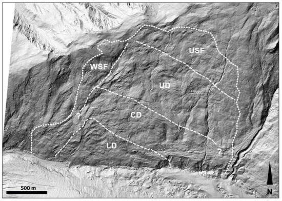
Figure 15.
Slope domain subdivision. UD: upper domain. CD: central domain. LD: lower domain. WSF: western secondary failure. USF: upper secondary failure.
The results of this research suggest that the complex geomorphic configuration of the Fels landslide is linked to the long-term evolution of the valley. Glacier retreat and the structural setting of the valley are the most significant factors in the occurrence and evolution of the landslide. The historical analysis documented a significant increase in surface cracking between 1977 and 1981, which is the time the Fels Glacier terminus retreated past the west boundary of the landslide area. The 30 m high step that marks the west boundary of the main landslide body (III in Figure 4 and Figure 10) is visible in the 1949 imagery, suggesting that the slope was moving before then. It can be argued that the Fels landslide is a reactivation of an older slope instability, which was possibly initiated at the end of the Pleistocene after the Cordilleran Ice Sheet disappeared and an alpine glacier became established in the Fels valley. However, the relatively low height and slope angle of the scarp and the absence of obvious landslide deposits on the valley floor in the Delta River valley suggest that the slope instability has never transitioned into a rapid rockslide or rock avalanche.
The impacts of glacier retreat on the stability of rock slopes have been extensively investigated, and many examples exist of instabilities that are initiated as a result of the down-wasting and recession of glaciers (e.g., [44,65,66,67]). However, the Fels landslide is peculiar, as it is the outcome of a series of events and processes that are connected by cause-and-effect links that enhance the kinematic freedom of the landslide. The historical aerial imagery shows that in 1949, displacements were concentrated on the lower slope. With glacier retreat, particularly since 1977, the fast-moving toe propagated upslope through a roto-translational or pseudo-rotational mechanism. Historic glacier retreat and the upslope propagation of the fast-moving toe induced (1) a decrease in lateral support of the landslide and (2) steepening of the lower slope. The weight of the material upslope of the fast-moving toe and decreased lateral support concentrated stresses at depth within the slope behind the fast-moving toe. This stress concentration appears to have been critical in the evolution of the landslide, as it led to the formation of a persistent multi-planar failure surface. The failure surface on the central and upper slope appears to exploit bedrock foliation (i.e., structural control on slope evolution), as its dip and dip direction are the same as the plunge and directions of surface displacement derived from the ST analysis. Based on the reconstructed profiles and assuming a constant orientation of the foliation, the rock mass must have been broken through for the failure surface to daylight near the valley floor. Stress concentration promotes this process, allowing the failure surface to propagate at a low angle within the lower slope and through the colluvial blanket by means of rock mass dilation, fracture propagation, and shearing of rock bridges. The multi-planar failure surface results in an “active-passive” configuration, in which the weight of the passive block lying on the low-angle part of the rupture surface opposes the displacement of an active block comprising material lying on the high-angle part of the failure surface. Yielding of the rock mass at the interface between active and passive blocks is a kinematic requirement for displacement of landslides with multi-planar failure surfaces [68]. In the case of the Fels landslide, accumulation of slope damage associated with the evolution of the fast-moving toe may have allowed the rock mass upslope to yield kinematically. The upslope propagation of the fast-moving toe, combined with the observed increase in displacement rates in the central and upper slope, appear to support this interpretation. Based on the combined results of our study, we classify the Fels landslide as a slow-moving, compound rockslide [33].
The role of earthquakes and ground shaking in the evolution and behavior of the Fels landslide is unclear. The Denali Fault, which ruptured during the 2002 earthquake, is located just a few kilometers south of the unstable slope. The intense ground shaking did not induce major deformation across the Fels landslide [32]. However, a coseismic surface scarp up to a few tens of centimeters high is present near the east boundary of the landslide. It is likely that coseismic slope damage, in the form of fracture propagation and cracking, may have also occurred at depth within the slope, potentially exacerbating seismic wave amplification in future earthquakes. Further, it is certain that future large earthquakes will occur on the Denali Fault, as it is a major locus of strain accumulation in Alaska [37]. Such damage accumulation and its effects are documented in the literature (e.g., [69], but its characterization in the field remains a challenge. The next stage in our Fels landslide investigation will include numerical modeling focused on the effects of both glacier retreat and ground shaking on the accumulation of internal slope damage and their role in the long-term geomorphic evolution and stability of the slope.
Another significant feature of this landslide is its displacement along a low-angle sliding surface. The factors that contribute to this low-angle surface are currently unclear. It is possible that damage during the earliest stages of the landslide, possibly combined with coseismic damage, decreased the strength available along the sliding surface, lowering its friction angle and cohesion to residual values. The presence of an elevated groundwater table may have also decreased shear strength, in combination with hydromechanical fatigue promoted by seasonal fluctuations. Nevertheless, in the absence of additional subsurface borehole data, these observations, although reasonable from a geomechanical viewpoint, remain speculative for this specific site.
The interpretation of the results obtained in this study is summarized using an “interaction matrix”, which graphically shows the role of selected controlling factors on the evolution, behavior, and stability of the Fels landslide (Figure 16). The use of interaction matrices in rock slope engineering was introduced by [70] and involves the development of a square matrix in which controlling factors are aligned along a diagonal. The off-diagonal cells (Xij) describe the effects of the interaction of the pair of controlling factors indicated by the row (i) and column (j) of the considered factors.
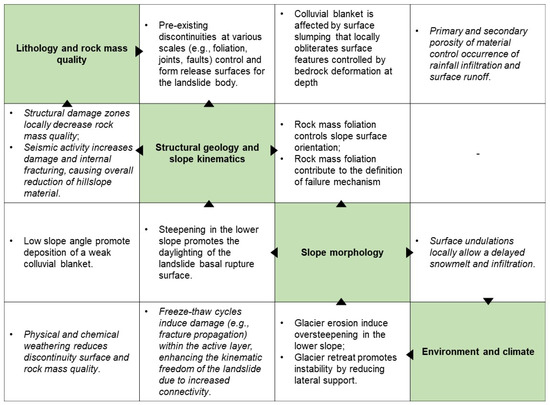
Figure 16.
Interaction matrix summarizing the role of selected principal controlling factors (green cells along the main diagonal) on the stability and evolution of the Fels landslide. Italic font indicates interactions that are assumed but have not been investigated in detail in the present research.
The workflow employed in this study involved a series of activities that can be performed independently before combining their results to provide a solid and geologically sound interpretation of the landslide. While the combination of field and remote sensing methods, including SAR-based monitoring, is often employed for landslide characterization and monitoring (Table 3), this is the first study that describes the application of the SAR ST method to perform long-term (10 years) monitoring of a large landslide and also to exploit the monitoring results to determine the mechanism of slope deformation and infer the morphology and depth of the basal surface. In particular, the use of the SAR ST technique provided estimates of the three components of the displacement vector to be estimated, which is critical in understanding the kinematic configuration of the landslide and its spatial variation across the unstable area. Despite its lower spatial resolution and accuracy compared to traditional InSAR techniques, the ability of SAR ST to document larger displacements both in the E-W and N-S directions were instrumental in characterizing the Fels landslide.
Table 3.
Selected published literature employing remote sensing methods, including SAR, to characterize and monitor landslides in rock.
6. Conclusions
Historical, field, and remote sensing data were acquired to characterize the deformation and failure mechanism of the Fels landslide. Historical aerial photographic imagery since 1949 was used to quantify glacier retreat and the progressive accumulation of surface cracking. Surface slope damage increased when the glacier terminus retreated past the west boundary of the landslide. ALS datasets were employed to map geomorphic lineaments across the landslide area, thus characterizing the structural setting of the slope and highlighting the occurrence of three major lineament trends aligned with the boundaries of the landslide. A significant correlation between the major lineament trends and outcrop-scale discontinuities was also noted. IRT was used to investigate the occurrence of seepage across the slope. An ST analysis was conducted using SAR imagery, and displacement trends, plunges, and magnitudes were derived from the N-S, E-W, and up–down components of the displacement vectors. Displacement data relative to two five-year time windows, namely 2010–2015 and 2015–2020, were derived. A comparison of these datasets showed an increase in displacement rates across the landslide area between 2010 and 2020. The Fels landslide can be classified as a slow-moving compound rockslide (according to [33]) that is displacing along a multi-planar failure surface that exploits bedrock foliation in the central and upper slope areas and is accompanied by rock mass yielding in the lower slope area. The landslide likely represents the reactivation of an older slope instability that was possibly initiated following late Pleistocene deglaciation and never transitioned from a slow creeping deformation to a rapid rockslide or rock avalanche. The style of deformation appears to be controlled by geological structures at different scales. This research provides evidence that ongoing climate change may potentially impact the evolution of the landslide. Specifically, it is shown that surface damage and cracking at the site progressed in combination with glacier thinning and retreat as a result of enhanced kinematic freedom of the slope.
The usefulness of the SAT ST technique for unstable slope characterization has been demonstrated. The main advantage of the work plan used in this study is that it allows researchers to determine geological and structural factors controlling the displacement of large, slow-moving landslides where subsurface or geophysical data are not available and site access is difficult due to challenging logistics or terrain. This research also demonstrated the potential practical applications of multi-temporal SAR ST datasets, not only for slope monitoring but also for characterizing the style of deformation and classifying the failure mechanism of slow-moving landslides. The main limitation of the approach employed in this study is related to its restricted applicability to slow rock slope deformations and displacements. Fast slope instabilities should be investigated and monitored using techniques that allow for more frequent surveys. Additionally, the resolution of the SAR ST datasets is lower than that of other satellite-based monitoring datasets such as InSAR. However, the employed approach is well suited for slow-moving landslides with large surface areas (several hundred square meters to several square kilometers), and a comparatively low resolution is still capable of describing and measuring slope movements with accuracy and a significant level of detail. Additionally, the subsurface configuration of the landslide remains a significant source of uncertainty, and engineering judgment remains important in the interpretation of the failure mechanism and the style of deformation. Nevertheless, this approach adopted in this study can assist in planning geophysical surveys and geotechnical borehole drilling, which, in turn, can confirm the location of the basal rupture surface.
The importance of historical datasets, such as air photographs and maps, for critically assessing the evolution of landslides, glaciers, and valley slopes over the past 100 years is emphasized in this study. Archived maps and air photographs will likely continue to be important resources for slope investigations, at least until several decades of historical LiDAR and SAR datasets become available.
The datasets collected and processed in this study will be instrumental for future numerical simulations of the landslide, which represents the next step in this research project. Numerical modeling is an important complement to any investigation of the long-term evolution of unstable slopes, as it allows the effects of slope damage accumulation due to glacier flow or seismic ground shaking to be determined. In this context, field and remote sensing data collected in this study will serve as input data for numerical modeling that will be conducted using sophisticated approaches, such as the distinct element method. Importantly, monitoring data, particularly SAR ST data, will also be valuable for constraining and validating the results of numerical simulations. Additional SAR ST analyses will also be conducted in order to establish trends of displacement of the landslide to improve understanding of the style of deformation and potential future evolution in terms of morphological changes and long-term stability.
Even if located in remote regions, large landslides can still affect people, either directly by endangering communities located near unstable slopes or indirectly by disrupting food, water, and power supply chains. Effectively characterizing and managing landslide risk requires identification and subsequent monitoring of unstable slopes using a combination of remote sensing methods.
Author Contributions
Conceptualization, D.D., D.S. and B.R.; methodology, D.D. and B.R.; formal analysis, D.D., J.E. and B.R.; investigation, D.D. and S.D.N.; writing—original draft preparation, D.D.; writing—review and editing, B.R., J.E., D.S., J.J.C., M.F. and S.D.N.; funding acquisition, D.S. and B.R.; supervision, D.S. and B.R. All authors have read and agreed to the published version of the manuscript.
Funding
The authors acknowledge the financial support provided through an NSERC Discovery Grant (ID: RGPIN 05817) and FRBC Endowment funds provided to Doug Stead. The speckle-tracking analysis part of this work was funded through the research program of the NSERC-MDA-CSA Industrial Research Chair in Synthetic Aperture Radar Technologies, Methods, and Applications (SAR Chair) at Simon Fraser University. The authors thank MDA Inc., through their in-kind support for the SAR Chair, for providing access to the high-resolution RADARSAT-2 data used for the speckle-tracking analysis.
Data Availability Statement
The data are not publicly available due to third-party restrictions and are partly available on reasonable request from the corresponding author.
Acknowledgments
We gratefully acknowledge Frank Wuttig (Trans-Alaska Pipeline Service Company) for providing the ALS datasets and helicopter access to the site. We also thank Franz Meyer of the University of Alaska Fairbanks for his assistance during this research and Jesse Mysiorek for assistance in the field.
Conflicts of Interest
J.E. was employed by the company BGC Engineering, Inc. The remaining authors declare that the research was conducted in the absence of any commercial or financial relationships that could be construed as a potential conflict of interest.
References
- Froude, M.J.; Petley, D.N. Global Fatal Landslide Occurrence from 2004 to 2016. Nat. Hazards Earth Syst. Sci. 2018, 18, 2161–2181. [Google Scholar] [CrossRef]
- Winter, M.G.; Shearer, B.; Palmer, D.; Peeling, D.; Harmer, C.; Sharpe, J. The Economic Impact of Landslides and Floods on the Road Network. Procedia Eng. 2016, 143, 1425–1434. [Google Scholar] [CrossRef]
- Shan, J.; Toth, C.K. Topographic Laser Ranging and Scanning. Principles and Processing; Taylor & Francis Group: Abingdon, UK, 2008; ISBN 978-1-4200-5142-1. [Google Scholar]
- Agliardi, F.; Crosta, G.B.; Meloni, F.; Valle, C.; Rivolta, C. Structurally-Controlled Instability, Damage and Slope Failure in a Porphyry Rock Mass. Tectonophysics 2013, 605, 34–47. [Google Scholar] [CrossRef]
- Stead, D.; Donati, D.; Wolter, A.; Sturzenegger, M. Application of Remote Sensing to the Investigation of Rock Slopes: Experience Gained and Lessons Learned. ISPRS Int. J. Geo-Inf. 2019, 8, 296. [Google Scholar] [CrossRef]
- Donati, D.; Westin, A.M.; Stead, D.; Clague, J.J.; Stewart, T.W.; Lawrence, M.S.; Marsh, J. A Reinterpretation of the Downie Slide (British Columbia, Canada) Based on Slope Damage Characterization and Subsurface Data Interpretation. Landslides 2021, 18, 1561–1583. [Google Scholar] [CrossRef]
- Francioni, M.; Salvini, R.; Stead, D.; Giovannini, R.; Riccucci, S.; Vanneschi, C.; Gullì, D. An Integrated Remote Sensing-GIS Approach for the Analysis of an Open Pit in the Carrara Marble District, Italy: Slope Stability Assessment through Kinematic and Numerical Methods. Comput. Geotech. 2015, 67, 46–63. [Google Scholar] [CrossRef]
- Donati, D.; Stead, D.; Lato, M.; Gaib, S. Spatio-Temporal Characterization of Slope Damage: Insights from the Ten Mile Slide, British Columbia, Canada. Landslides 2020, 17, 1037–1049. [Google Scholar] [CrossRef]
- Jaboyedoff, M.; Derron, M.-H. Chapter 7—Landslide Analysis Using Laser Scanners. In Developments in Earth Surface Processes; Tarolli, P., Mudd, S.M., Eds.; Remote Sensing of Geomorphology; Elsevier: Amsterdam, The Netherlands, 2020; Volume 23, pp. 207–230. [Google Scholar]
- Lindner, G.; Schraml, K.; Mansberger, R.; Hübl, J. UAV Monitoring and Documentation of a Large Landslide. Appl. Geomat. 2016, 8, 1–11. [Google Scholar] [CrossRef]
- Francioni, M.; Coggan, J.; Eyre, M.; Stead, D. A Combined Field/Remote Sensing Approach for Characterizing Landslide Risk in Coastal Areas. Int. J. Appl. Earth Obs. Geoinf. 2018, 67, 79–95. [Google Scholar] [CrossRef]
- Casagli, N.; Frodella, W.; Morelli, S.; Tofani, V.; Ciampalini, A.; Intrieri, E.; Raspini, F.; Rossi, G.; Tanteri, L.; Lu, P. Spaceborne, UAV and Ground-Based Remote Sensing Techniques for Landslide Mapping, Monitoring and Early Warning. Geoenviron. Disasters 2017, 4, 9. [Google Scholar] [CrossRef]
- Walton, G.; Christiansen, C.; Kromer, R.; Silaev, A. Evaluation of Rockfall Trends at a Sedimentary Rock Cut near Manitou Springs, Colorado, Using Daily Photogrammetric Monitoring. Landslides 2023, 20, 2657–2674. [Google Scholar] [CrossRef]
- Westoby, M.J.; Brasington, J.; Glasser, N.F.; Hambrey, M.J.; Reynolds, J.M. "Structure-from-Motion" Photogrammetry: A Low-Cost, Effective Tool for Geoscience Applications. Geomorphology 2012, 179, 300–314. [Google Scholar] [CrossRef]
- Sturzenegger, M.; Stead, D. Close-Range Terrestrial Digital Photogrammetry and Terrestrial Laser Scanning for Discontinuity Characterization on Rock Cuts. Eng. Geol. 2009, 106, 163–182. [Google Scholar] [CrossRef]
- Teza, G.; Marcato, G.; Pasuto, A.; Galgaro, A. Integration of Laser Scanning and Thermal Imaging in Monitoring Optimization and Assessment of Rockfall Hazard: A Case History in the Carnic Alps (Northeastern Italy). Nat. Hazards 2015, 76, 1535–1549. [Google Scholar] [CrossRef]
- Franzosi, F.; Crippa, C.; Derron, M.-H.; Jaboyedoff, M.; Agliardi, F. Slope-Scale Remote Mapping of Rock Mass Fracturing by Modeling Cooling Trends Derived from Infrared Thermography. Remote Sens. 2023, 15, 4525. [Google Scholar] [CrossRef]
- Kurz, T.H.; Buckley, S.J.; Howell, J. A Close-Range Hyperspectral Imaging for Geological Field Studies: Workflow and Methods. Int. J. Remote Sens. 2013, 34, 1798–1822. [Google Scholar] [CrossRef]
- Kromer, R.A.; Abellán, A.; Hutchinson, D.J.; Lato, M.; Chanut, M.-A.; Dubois, L.; Jaboyedoff, M. Automated Terrestrial Laser Scanning with Near-Real-Time Change Detection—Monitoring of the Séchilienne Landslide. Earth Surf. Dyn. 2017, 5, 293–310. [Google Scholar] [CrossRef]
- Williams, J.G.; Rosser, N.J.; Hardy, R.J.; Brain, M.J.; Afana, A.A. Optimising 4-D Surface Change Detection: An Approach for Capturing Rockfall Magnitude–Frequency. Earth Surf. Dyn. 2018, 6, 101–119. [Google Scholar] [CrossRef]
- Kromer, R.; Walton, G.; Gray, B.; Lato, M.; Group, R. Development and Optimization of an Automated Fixed-Location Time Lapse Photogrammetric Rock Slope Monitoring System. Remote Sens. 2019, 11, 1890. [Google Scholar] [CrossRef]
- Colesanti, C.; Wasowski, J. Investigating Landslides with Space-Borne Synthetic Aperture Radar (SAR) Interferometry. Eng. Geol. 2006, 88, 173–199. [Google Scholar] [CrossRef]
- Sharifi, S.; Macciotta, R.; Hendry, M.; Rotheram-Clarke, D.; Huntley, D. Evaluating Topography-Based Methods in 3D Decomposition of InSAR 1D Velocities Obtained for Translational Landslides: Thompson River Valley in Canada. Landslides 2023. [Google Scholar] [CrossRef]
- Yao, J.; Yao, X.; Liu, X. Landslide Detection and Mapping Based on SBAS-InSAR and PS-InSAR: A Case Study in Gongjue County, Tibet, China. Remote Sens. 2022, 14, 4728. [Google Scholar] [CrossRef]
- Wright, T.J.; Parsons, B.E.; Lu, Z. Toward Mapping Surface Deformation in Three Dimensions using InSAR. Geophys. Res. Lett. 2004, 31, 169–178. [Google Scholar] [CrossRef]
- Jo, M.J.; Jung, H.S.; Won, J.S.; Poland, M.P.; Miklius, A.; Lu, Z. Measurement of Slow-Moving along-Track Displacement from an Efficient Multiple-Aperture SAR Interferometry (MAI) Stacking. J. Geod. 2015, 89, 411–425. [Google Scholar] [CrossRef]
- Isya, N.H.; Niemeier, W.; Gerke, M. 3D Estimation of Slow Ground Motion using InSAR and the Slope Aspect Assumption, a Case Study: The Puncak Pass Landslide, Indonesia. ISPRS Ann. Photogramm. Remote Sens. Spat. Inf. Sci. 2019, IV-2/W5, 623–630. [Google Scholar] [CrossRef]
- Raspini, F.; Ciampalini, A.; Conte, S.D.; Lombardi, L.; Nocentini, M.; Gigli, G.; Ferretti, A.; Casagli, N. Exploitation of Amplitude and Phase of Satellite SAR Images for Landslide Mapping: The Case of Montescaglioso (South Italy). Remote Sens. 2015, 7, 14576–14596. [Google Scholar] [CrossRef]
- Teza, G.; Atzeni, C.; Balzani, M.; Galgaro, A.; Galvani, G.; Genevois, R.; Luzi, G.; Mecatti, D.; Noferini, L.; Pieraccini, M.; et al. Ground-based Monitoring of High-risk Landslides through joint use of Laser Scanner and Interferometric Radar. Int. J. Remote Sens. 2008, 29, 4735–4756. [Google Scholar] [CrossRef]
- Agliardi, F.; Crosta, G.B.; Frattini, P.; Malusà, M.G. Giant Non-Catastrophic Landslides and the Long-Term Exhumation of the European Alps. Earth Planet. Sci. Lett. 2013, 365, 263–274. [Google Scholar] [CrossRef]
- Donati, D.; Rabus, B.; Engelbrecht, J.; Stead, D.; Clague, J.; Francioni, M. A Robust SAR Speckle Tracking Workflow for Measuring and Interpreting the 3D Surface Displacement of Landslides. Remote Sens. 2021, 13, 3048. [Google Scholar] [CrossRef]
- Newman, S.D. Deep-Seated Gravitational Slope Deformations Near the Trans-Alaska Pipeline, East-Central Alska Range. Master’s Thesis, Simon Fraser University, Burnaby, BC, Canada, 2013. [Google Scholar]
- Hungr, O.; Leroueil, S.; Picarelli, L. The Varnes Classification of Landslide Types, an Update. Landslides 2014, 11, 167–194. [Google Scholar] [CrossRef]
- Nokleberg, W.J.; Aleinikoff, J.N. Summary of Stratigraphy, Structure, and Metamorphism of Devonian Igneous-Arc Terranes, Northeastern Mount Hayes Quadrangle, Eastern Alaskan Range. In The United States Geological Survey in Alaska; Accomplishments during 1984: U.S. Geological Survey Circular 967; U.S. Geological Survey: Reston, VA, USA, 1985. [Google Scholar]
- Nokleberg, W.J.; Aleinikoff, J.N.; Bond, G.C.; Ferrians, O.J.; Herzon, P.L.; Lange, I.M.; Miyaoka, R.T.; Richter, D.H.; Schwab, C.E.; Silva, S.R.; et al. Geologic Maps of the Eastern Alaska Range, Alaska (44 Quadrangles, 1:63,360 Scale), with Descriptions and Interpretations of Map Units: Alaska Division of Geological & Geophysical Surveys Report of Investigation; Alaska Division of Geological & Geophysical Surveys: College, AK, USA, 2015.
- Eberhart-Phillips, D.; Haeussler, P.J.; Freymueller, J.T.; Frankel, A.D.; Rubin, C.M.; Craw, P.; Ratchkovski, N.A.; Anderson, G.; Carver, G.A.; Crone, A.J.; et al. The 2002 Denali Fault Earthquake, Alaska: A Large Magnitude, Slip-Partitioned Event. Science 2003, 300, 1113–1118. [Google Scholar] [CrossRef]
- Haeussler, P.J. Surface Rupture and Slip Distribution of the Denali and Totschunda Faults in the 3 November 2002 M 7.9 Earthquake, Alaska. Bull. Seismol. Soc. Am. 2004, 94, S23–S52. [Google Scholar] [CrossRef]
- Jibson, R.W.; Harp, E.L.; Schulz, W.; Keefer, D.K. Landslides Triggered by the 2002 Denali Fault, Alaska, Earthquake and the Inferred Nature of the Strong Shaking. Earthq. Spectra 2004, 20, 669–691. [Google Scholar] [CrossRef]
- Jibson, R.W.; Harp, E.L.; Schulz, W.; Keefer, D.K. Large Rock Avalanches Triggered by the M 7.9 Denali Fault, Alaska, Earthquake of 3 November 2002. Eng. Geol. 2006, 83, 144–160. [Google Scholar] [CrossRef]
- Grantz, A.; Plafker, G.; Kachadoorian, R. Alaska’s Good Friday Earthquake, March 27, 1964: A Preliminary Geologic Evaluation; Geolological Survey Circular 491; U.S. Department of the Interior, Geological Survey: Washington, DC, USA, 1964; pp. 1–35. [CrossRef]
- Planet Team Planet Application Program Interface: In Space for Life on Earth. San Francisco, CA. 2019. Available online: https://developers.planet.com (accessed on 1 July 2023).
- Grämiger, L.M.; Moore, J.R.; Gischig, V.S.; Ivy-Ochs, S.; Loew, S. Beyond Debuttressing: Mechanics of Paraglacial Rock Slope Damage during Repeat Glacial Cycles. J. Geophys. Res. Earth Surf. 2017, 122, 1004–1036. [Google Scholar] [CrossRef]
- Kos, A.; Amann, F.; Strozzi, T.; Delaloye, R.; von Ruette, J.; Springman, S. Contemporary Glacier Retreat Triggers a Rapid Landslide Response, Great Aletsch Glacier, Switzerland. Geophys. Res. Lett. 2016, 43, 12, 412–466, 474. [Google Scholar] [CrossRef]
- Clayton, A.; Stead, D.; Kinakin, D.; Wolter, A. Engineering Geomorphological Interpretation of the Mitchell Creek Landslide, British Columbia, Canada. Landslides 2017, 14, 1655–1675. [Google Scholar] [CrossRef]
- Donati, D.; Stead, D.; Brideau, M.A.; Ghirotti, M. Using Pre-Failure and Post-Failure Remote Sensing Data to Constrain the Three-Dimensional Numerical Model of a Large Rock Slope Failure. Landslides 2021, 18, 827–847. [Google Scholar] [CrossRef]
- Howley, M.W. A Late Glacial and Holocene Chronology of the Castner Glacier, Delta River Valley, Alaska. Master’s Thesis, University of New Hampshire, Durham, NH, USA, 2008. [Google Scholar]
- Sharma, J.; Busler, J.; Francioni, M.; Stead, D.; Donati, D.; Onsel, E.; Clague, J.J.; Brideau, M.A. Monitoring Landslides along Pipeline Corridors using a Combined Satellite-Based InSAR and Geomechanical Modelling Approach. In Proceedings of the 69th Canadian Geotechnical Conference, Vancouver, BC, Canada, 2–5 October 2016. [Google Scholar]
- Hoek, E.; Brown, E.T. Practical Estimates of Rock Mass Strength. Int. J. Rock Mech. Min. Sci. 1997, 34, 1165–1186. [Google Scholar] [CrossRef]
- Hoek, E.; Brown, E.T. The Hoek–Brown Failure Criterion and GSI—2018 Edition. J. Rock Mech. Geotech. Eng. 2019, 11, 445–463. [Google Scholar] [CrossRef]
- Barton, N.R. ISRM Suggested Methods for the Quantitative Description of Discontinuities in Rock Masses. Int. J. Rock Mech. Min. Sci. Geomech. Abstr. 1978, 15, 319–368. [Google Scholar] [CrossRef]
- ESRI ArcMap 10.6. 2019. Available online: https://www.esri.com/ (accessed on 15 March 2023).
- Francioni, M.; Stead, D.; Clague, J.J.; Westin, A. Identification and Analysis of Large Paleo-Landslides at Mount Burnaby, British Columbia. Environ. Eng. Geosci. 2018, 24, 221–235. [Google Scholar] [CrossRef]
- Stead, D.; Wolter, A. A Critical Review of Rock Slope Failure Mechanisms: The Importance of Structural Geology. J. Struct. Geol. 2015, 74, 1–23. [Google Scholar] [CrossRef]
- Rocscience DIPS. 2022. Available online: https://www.rocscience.com/software/dips (accessed on 15 March 2023).
- Brideau, M.-A.; Yan, M.; Stead, D. The Role of Tectonic Damage and Brittle Rock Fracture in the Development of Large Rock Slope Failures. Geomorphology 2009, 103, 30–49. [Google Scholar] [CrossRef]
- FLIR ResearchIR. 2019. Available online: https://www.flir.com/support-center/Instruments/researchir/ (accessed on 15 March 2023).
- CloudCompare 2.12 [GPL Software]. 2022. Available online: https://www.danielgm.net/cc/ (accessed on 15 March 2023).
- Intrieri, E.; Frodella, W.; Raspini, F.; Bardi, F.; Tofani, V. Using Satellite Interferometry to Infer Landslide Sliding Surface Depth and Geometry. Remote Sens. 2020, 12, 1462. [Google Scholar] [CrossRef]
- Wood, F.B. Global Alpine Glacier Trends, 1960s to 1980s. Arct. Alp. Res. 1988, 20, 404–413. [Google Scholar] [CrossRef]
- Molnia, B.F. Late Nineteenth to Early Twenty-First Century Behavior of Alaskan Glaciers as Indicators of Changing Regional Climate. Glob. Planet. Chang. 2007, 56, 23–56. [Google Scholar] [CrossRef]
- Koch, J.; Menounos, B.; Clague, J.J. Glacier Change in Garibaldi Provincial Park, Southern Coast Mountains, British Columbia, since the Little Ice Age. Glob. Planet. Chang. 2009, 66, 161–178. [Google Scholar] [CrossRef]
- Sturzenegger, M.; Stead, D.; Elmo, D. Terrestrial Remote Sensing-Based Estimation of Mean Trace Length, Trace Intensity and Block Size/Shape. Eng. Geol. 2011, 119, 96–111. [Google Scholar] [CrossRef]
- Boncori, J.P.M. Measuring Coseismic Deformation with Spaceborne Synthetic Aperture Radar: A Review. Front. Earth Sci. 2019, 7, 1–20. [Google Scholar] [CrossRef]
- Rocscience SWEDGE. 2022. Available online: https://www.rocscience.com/software/swedge (accessed on 15 March 2023).
- Holm, K.; Bovis, M.; Jakob, M. The Landslide Response of Alpine Basins to Post-Little Ice Age Glacial Thinning and Retreat in Southwestern British Columbia. Geomorphology 2004, 57, 201–216. [Google Scholar] [CrossRef]
- Riva, F.; Agliardi, F.; Amitrano, D.; Crosta, G.B. Damage-Based Time-Dependent Modeling of Paraglacial to Postglacial Progressive Failure of Large Rock Slopes. J. Geophys. Res. Earth Surf. 2018, 123, 124–141. [Google Scholar] [CrossRef]
- Roberti, G.; Ward, B.; van Wyk de Vries, B.; Friele, P.; Perotti, L.; Clague, J.J.; Giardino, M. Precursory Slope Distress Prior to the 2010 Mount Meager Landslide, British Columbia. Landslides 2018, 15, 637–647. [Google Scholar] [CrossRef]
- Kvapil, R.; Clews, M. An Examination of the Prandtl Mechanism in Large Dimension Slope Failures. Trans. Inst. Min. Metall. Sect. A 1979, 88, A1–A5. [Google Scholar]
- Gischig, V.S.; Eberhardt, E.; Moore, J.R.; Hungr, O. On the Seismic Response of Deep-Seated Rock Slope Instabilities—Insights from Numerical Modeling. Eng. Geol. 2015, 193, 1–18. [Google Scholar] [CrossRef]
- Hudson, J.A. Rock Engineering Systems—Theory and Practice; Ellis Horwood Limited: Hemel Hempstead, UK, 1992. [Google Scholar]
- Barla, G.; Antolini, F.; Barla, M.; Mensi, E.; Piovano, G. Monitoring of the Beauregard Landslide (Aosta Valley, Italy) Using Advanced and Conventional Techniques. Eng. Geol. 2010, 116, 218–235. [Google Scholar] [CrossRef]
- Ambrosi, C.; Crosta, G.B. Large Sackung along Major Tectonic Features in the Central Italian Alps. Eng. Geol. 2006, 83, 183–200. [Google Scholar] [CrossRef]
- Ganerød, G.V.; Grøneng, G.; Rønning, J.S.; Dalsegg, E.; Elvebakk, H.; Tønnesen, J.F.; Kveldsvik, V.; Eiken, T.; Blikra, L.H.; Braathen, A. Geological Model of the Åknes Rockslide, Western Norway. Eng. Geol. 2008, 102, 1–18. [Google Scholar] [CrossRef]
- Kristensen, L.; Rivolta, C.; Dehles, J.; Blikra, L.H. GB Insar Measurement at the Åknes Rockslide, Norway. Ital. J. Eng. Geol. Environ. 2013, 339–348. [Google Scholar] [CrossRef]
- Prager, C.; Zangerl, C.; Nagler, T. Geological Controls on Slope Deformations in the Kofels Rockslide Area (Tyrol, Austria). Austrian J. Earth Sci. 2009, 102, 4–19. [Google Scholar]
- Eriksen, H.Ø.; Lauknes, T.R.; Larsen, Y.; Corner, G.D.; Bergh, S.G.; Dehls, J.; Kierulf, H.P. Visualizing and Interpreting Surface Displacement Patterns on Unstable Slopes Using Multi-Geometry Satellite SAR Interferometry (2D InSAR). Remote Sens. Environ. 2017, 191, 297–312. [Google Scholar] [CrossRef]
- Vick, L.M.; Böhme, M.; Rouyet, L.; Bergh, S.G.; Corner, G.D.; Lauknes, T.R. Structurally Controlled Rock Slope Deformation in Northern Norway. Landslides 2020, 17, 1745–1776. [Google Scholar] [CrossRef]


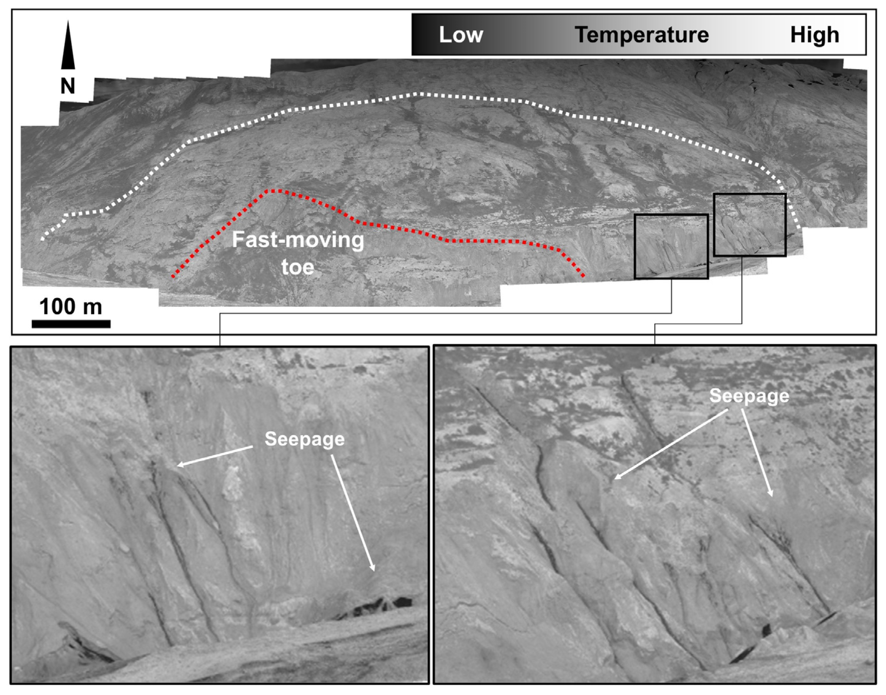
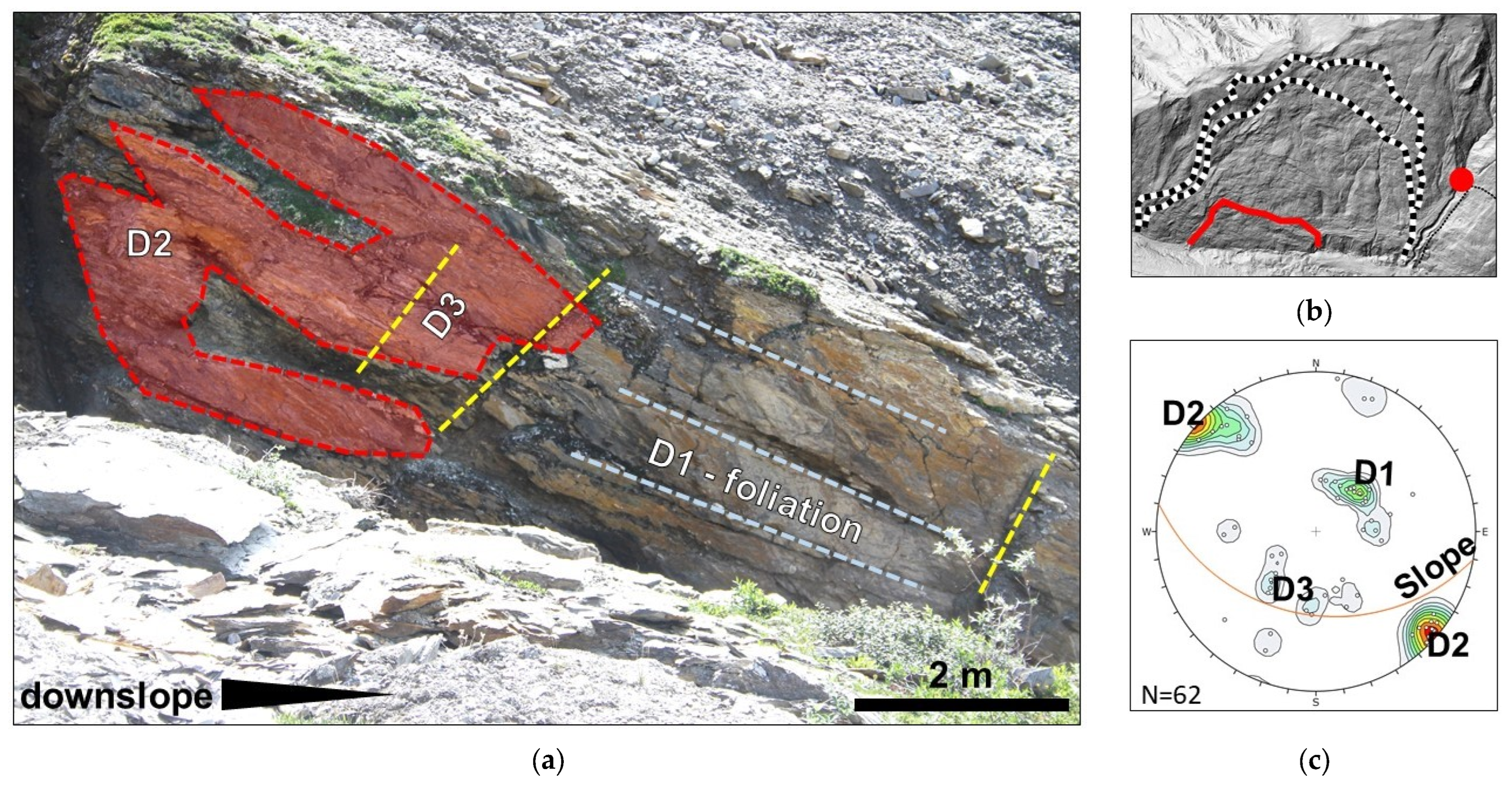
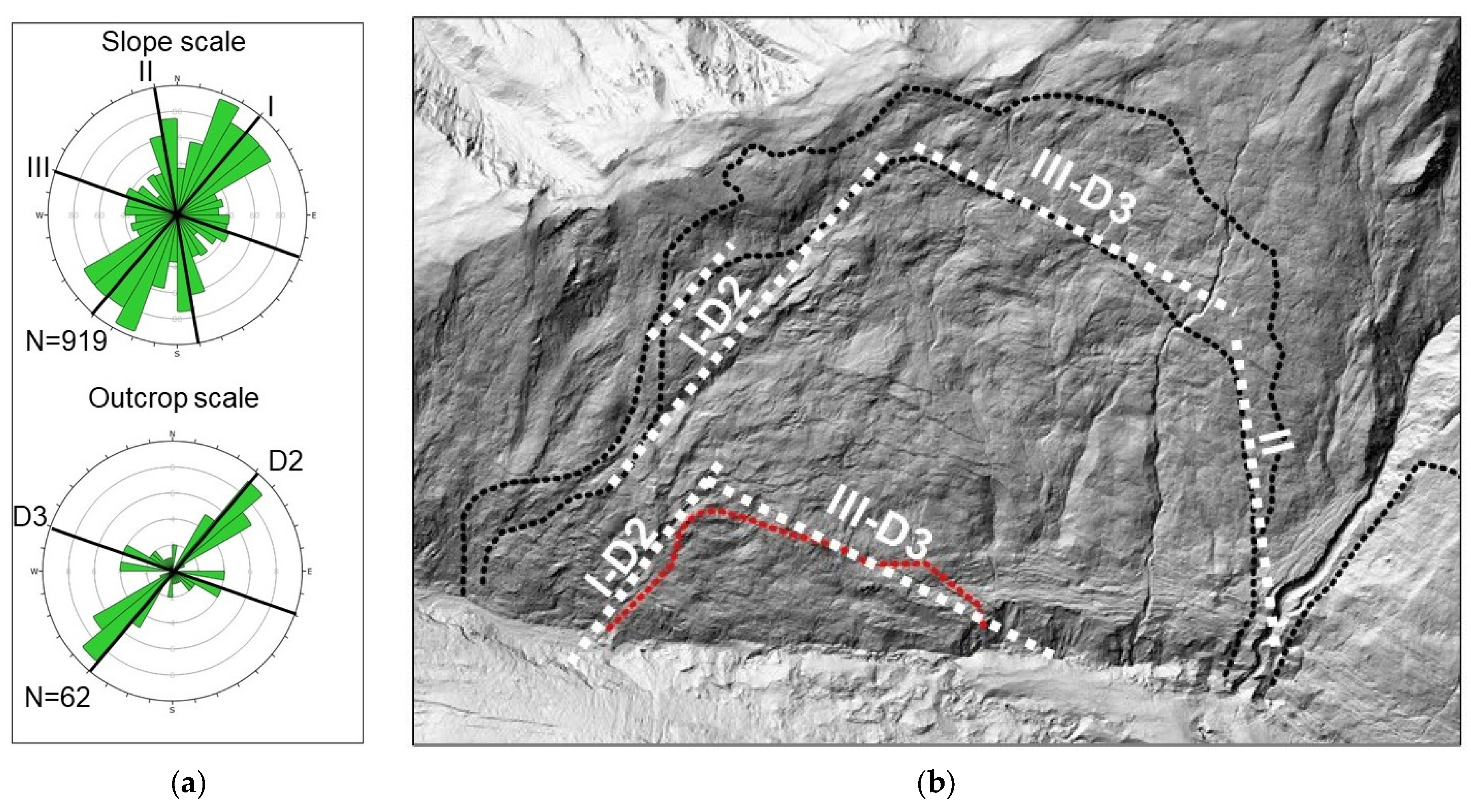

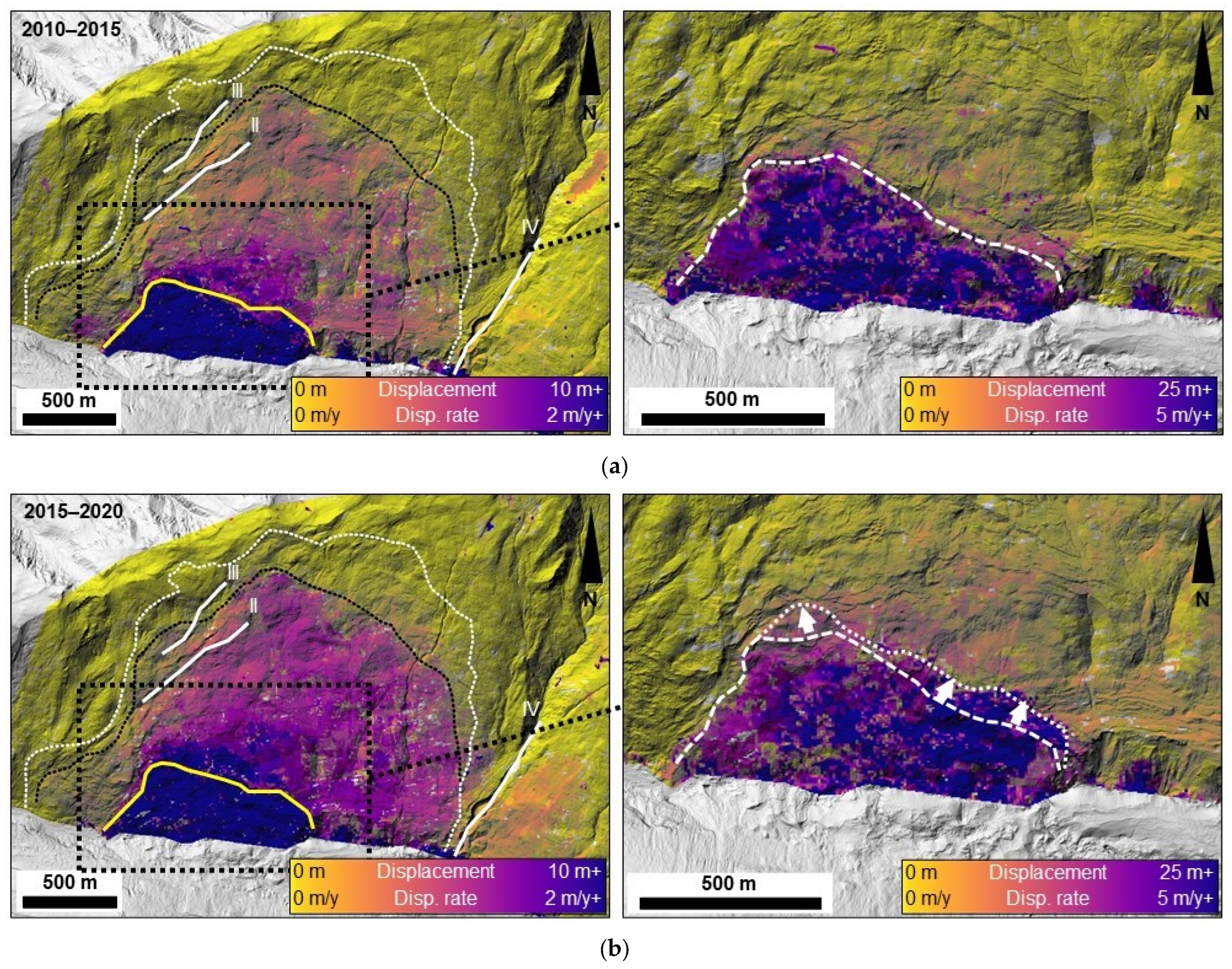
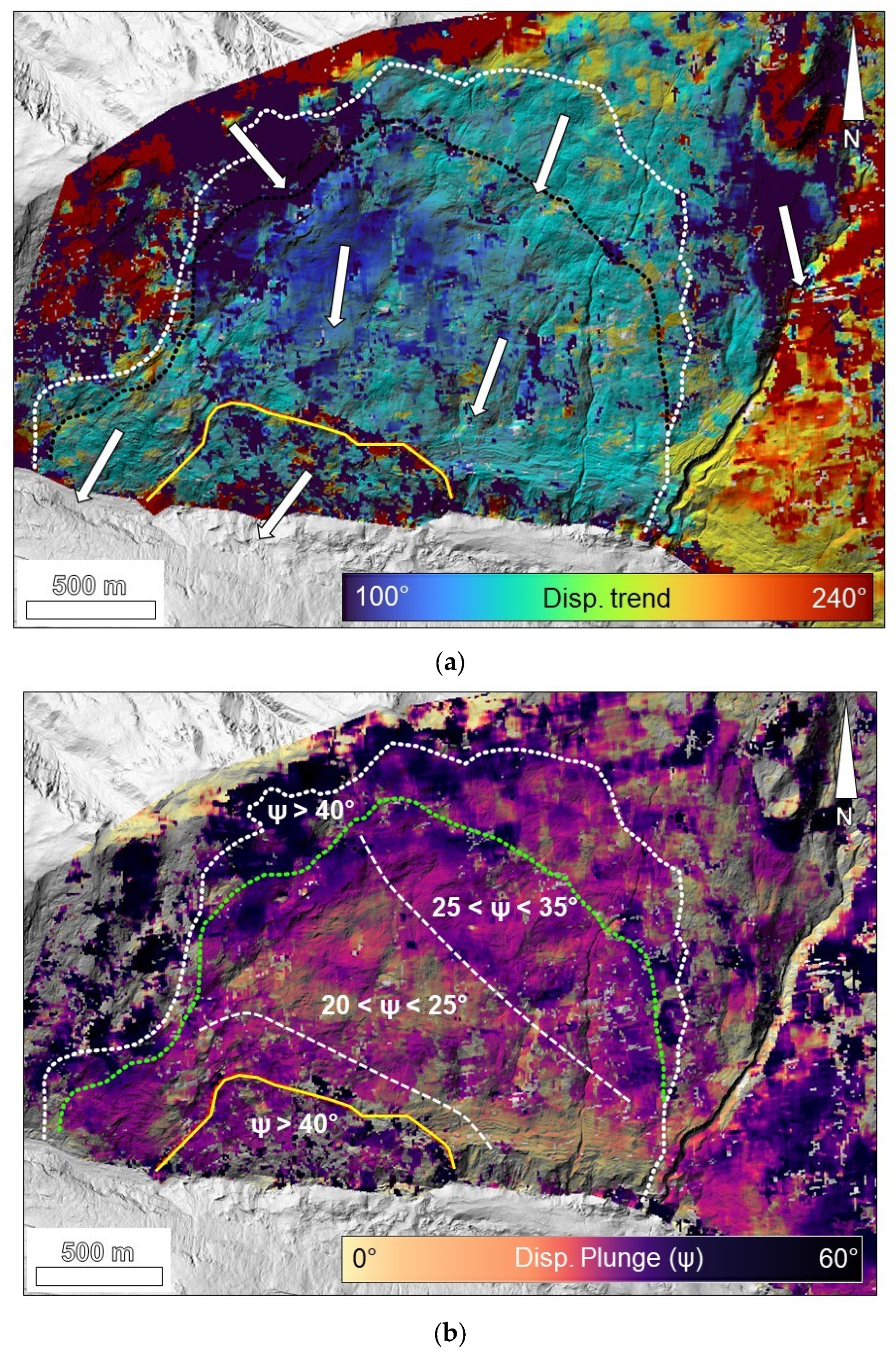

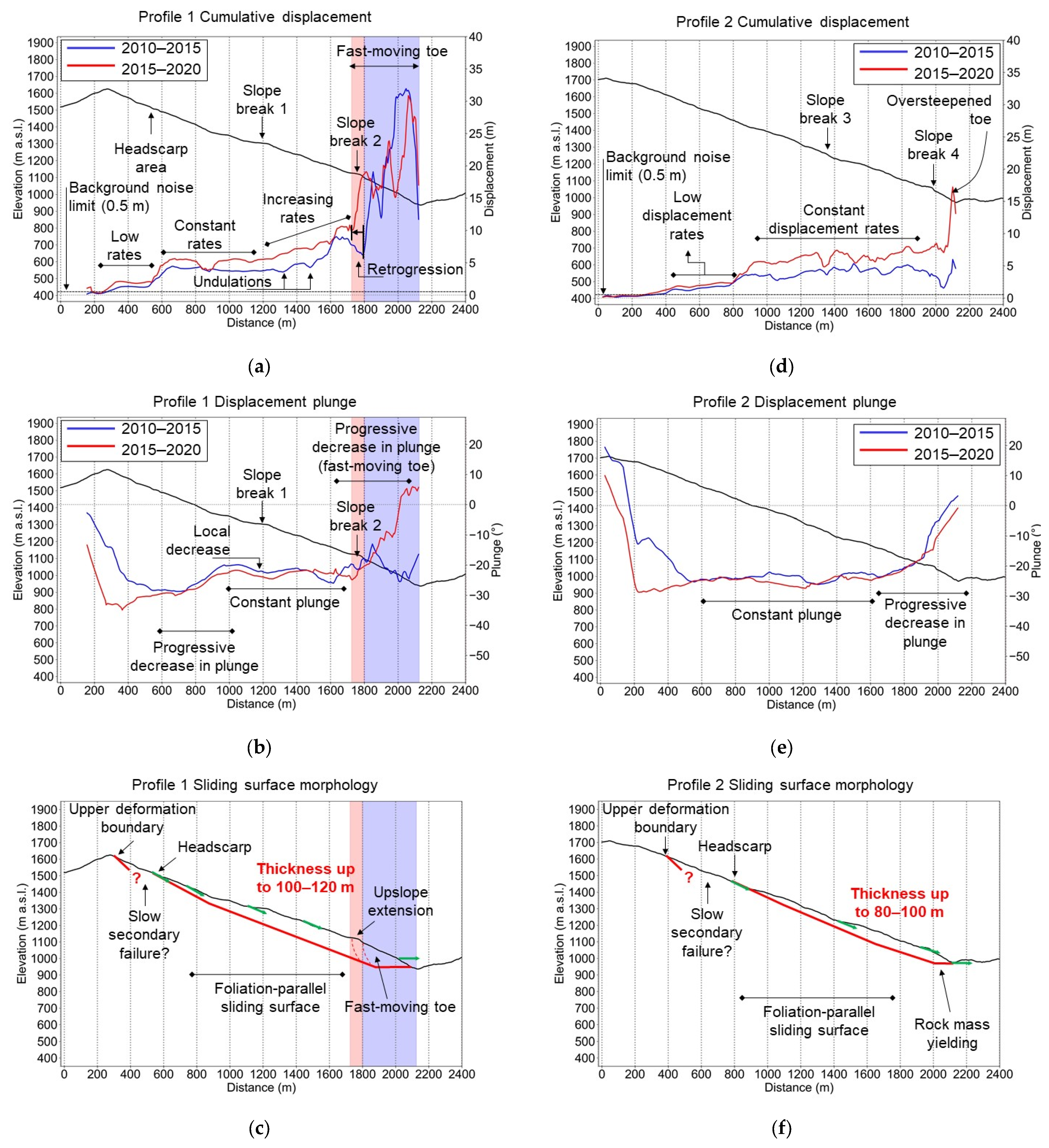
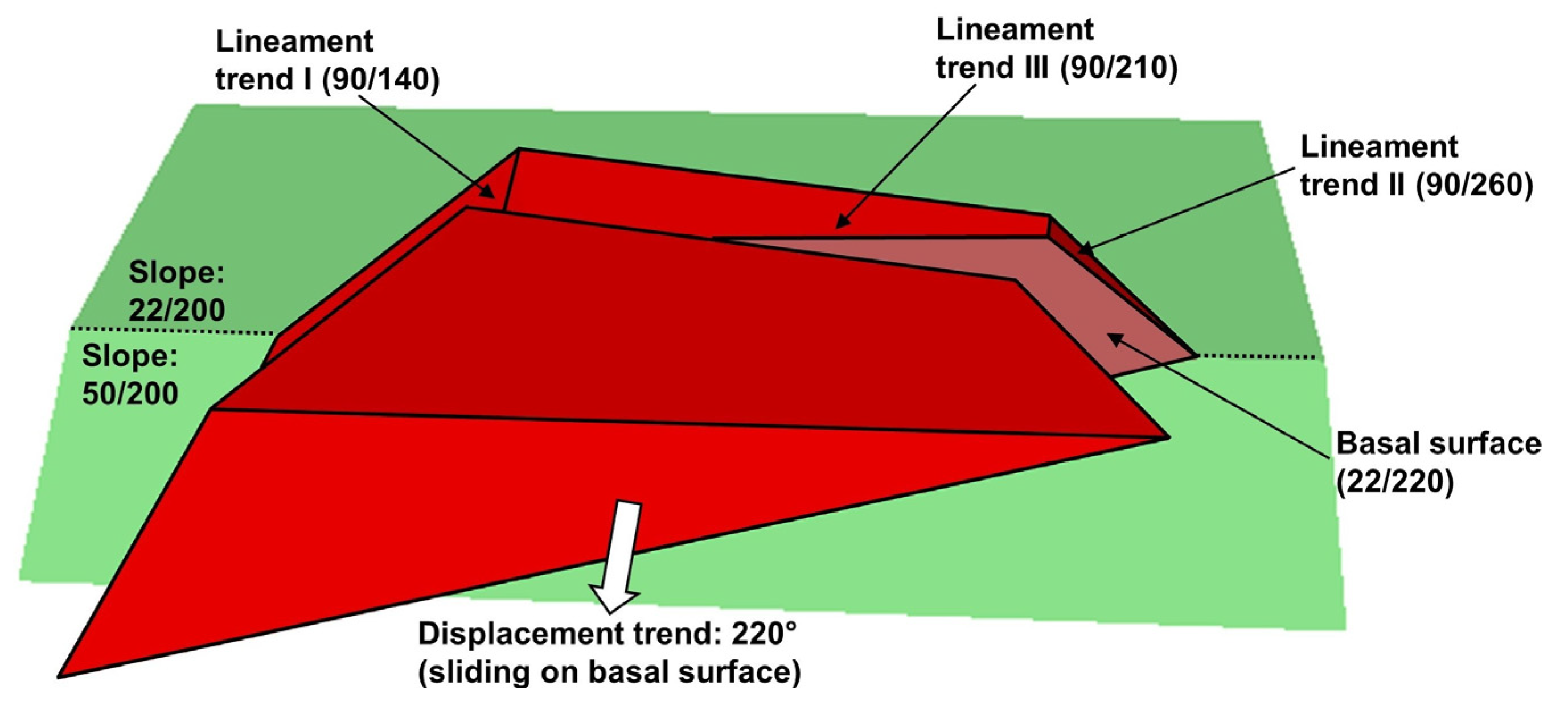

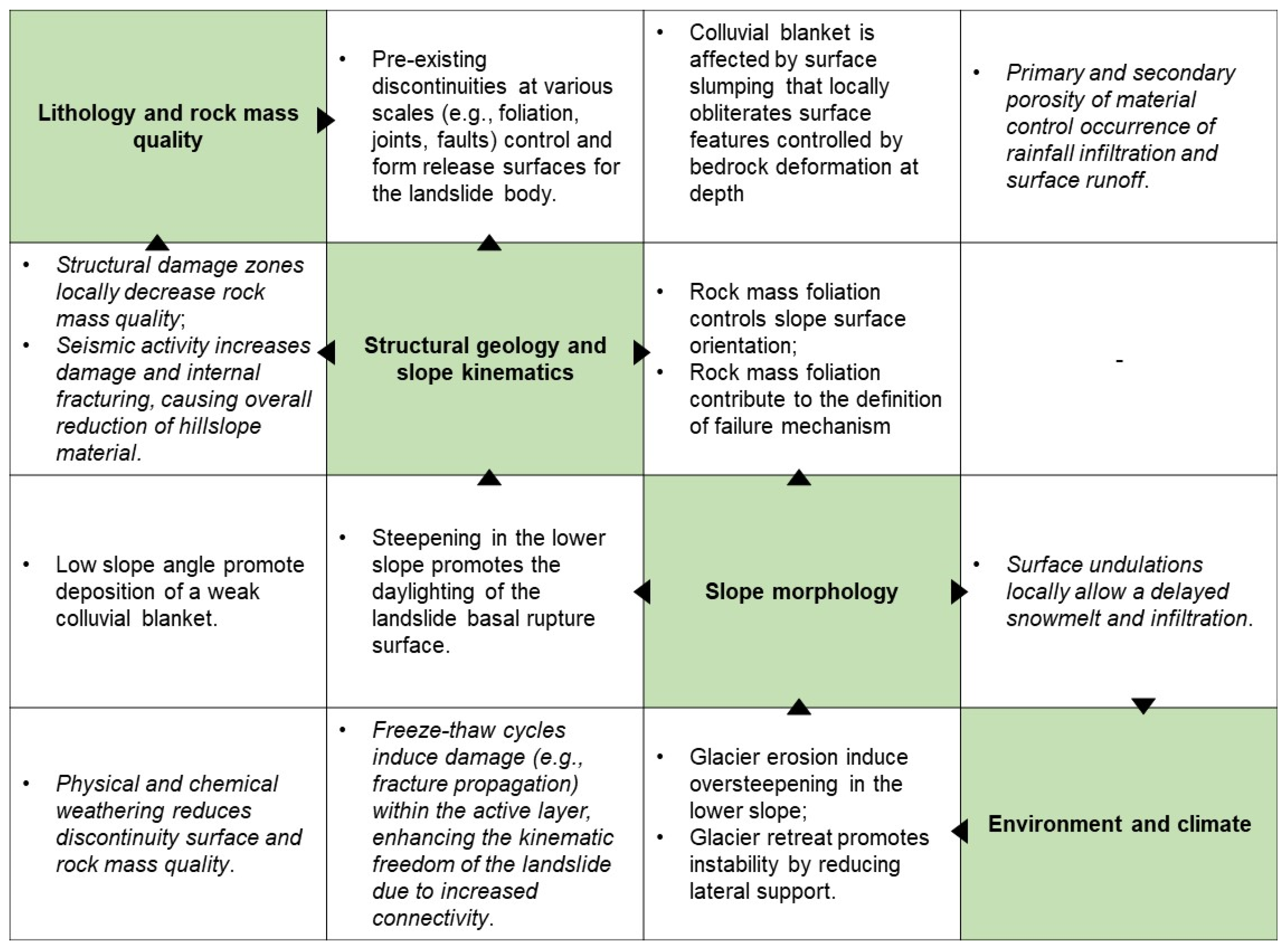
Disclaimer/Publisher’s Note: The statements, opinions and data contained in all publications are solely those of the individual author(s) and contributor(s) and not of MDPI and/or the editor(s). MDPI and/or the editor(s) disclaim responsibility for any injury to people or property resulting from any ideas, methods, instructions or products referred to in the content. |
© 2023 by the authors. Licensee MDPI, Basel, Switzerland. This article is an open access article distributed under the terms and conditions of the Creative Commons Attribution (CC BY) license (https://creativecommons.org/licenses/by/4.0/).