Abstract
As a typical application of geodesy, the GNSS/INS (Global Navigation Satellite System and Inertial Navigation System) integrated navigation technique was developed and has been applied for decades. For the integrated systems with multiple sensors, data fusion is one of the key problems. As a well-known data fusion algorithm, the Kalman filter can provide optimal estimates with known parameters of the models and noises. In the literature, however, the data fusion algorithm of the GNSS/INS integrated navigation and positioning systems is performed under a certain norm, and performance of the conventional filtering algorithms are improved only under this fixed and limited frame. The mixed norm-based data fusion algorithm is rarely discussed. In this paper, a mixed norm-based data fusion algorithm is proposed, and the hypothesis test statistics are constructed and adopted based on the chi-square distribution. Using the land vehicle data collected through the multi-GNSS and the IMU (Inertial Measurement Unit), the proposed algorithm is tested and compared with the conventional filtering algorithms. Results show that the influences of the outlying measurements and the uncertain noises are weakened with the proposed data fusion algorithm, and the precision of the estimates is further improved. Meanwhile, the proposed algorithm provides an open issue for geodetic applications with mixed norms.
1. Introduction
It is well known that GNSS is able to provide precise information of the position and velocity under a favorable observation environment, and the positioning errors do not accumulate over time. Thus, the GNSS technique has been applied in broad fields for many years [1,2,3]. Although different satellite navigation and positioning systems can be selected and the number of visible satellites is increasing, the performance of GNSS can be degraded by the signal problems, such as the lock-lost and unknown interferences. On the other hand, no signal is sent and received by INS, and it has been widely applied in the navigation of kinematic carriers. INS can provide precise and short-term navigation and positioning information, and the observation frequency is much higher than that of the GNSS receivers. Moreover, INS has many other advantages such as anti-electronic jamming. Nevertheless, the positioning errors of INS accumulate quickly over time [4], especially for the low-cost IMU, hence it cannot independently undertake the task of long-term navigation under fast kinematic conditions. Naturally, the properties of GNSS and INS are complementary, and the integrated systems provide an ideal solution in kinematic positioning and navigation applications [5,6,7].
One of the most imperative techniques for the GNSS/INS integrated navigation systems lies in the data fusion, and the most frequently used data fusion recursive algorithm for the discrete linear system is the Kalman filter [8,9]. In the Kalman filter, the estimates are optimal when the models and statistical information of the noises are exactly known. However, in the practical applications of the Kalman filter, the prior models and statistical information of the noises can hardly be specified due to the complex environment and uncertain circumstances. Thus, some outlying measurements and uncertain errors may significantly degrade the performance of the filtering. Moreover, the conventional Kalman filter is applicable for linear systems only, but more systems in practice exert nonlinear characters [10]. Aimed at addressing the shortcomings of the conventional Kalman filter, many types of filters were developed in practical applications. These improved filters mainly consist of nonlinear filters, robust filters and adaptive filters, et al. The extended Kalman filter (EKF) was proposed to deal with the nonlinear problem, and it is one of the most commonly used nonlinear Kalman filters. Proximate with the EKF, other types of nonlinear filters were proposed based on different norms, such as the particle filter [11], the unscented Kalman filter (UKF) [12] and the cubature Kalman filter (CKF) [13,14], et al. The central difference is that the Kalman filter (CDKF) can also conduct the nonlinear transformation by polynomial fitting [15]. With these nonlinear filters, the applications of the Kalman filter are extended further. The outlier detection method was developed to control the influences of the outlying measurements with a relatively low efficiency [16]. Then, the detection, identification and adaptation, namely, the D.I.A. methods were developed [17], but the process of identification is still a difficult problem. Based on the robust estimation theory and other robust algorithms, the robust filter was developed to weaken the influences of the outliers by the covariance inflation factor [18].
In terms of the model errors and the uncertain noises, a series of adaptive filters were developed. For the adaptive filters, the function model-based and the stochastic model-based adaptive filters are conventional solutions. Then, the multiple model-based and the innovation-based adaptive estimation were developed and applied in the GNSS/INS integrated navigation systems [19]. Furthermore, Chinese researchers developed a different type of adaptive filter through the adaptive factor [20], and four different factors and detection statistics were constructed and applied in the kinematic navigation and positioning field. Similarly, the finite impulse response filter was developed against the model errors. This filter requires no noise statistics and is not so sensitive to the model errors [21]. The centroid weighted Kalman filter is another improved filter aimed at the state model and the observation model uncertainty, and the centroid weighted method is applied to optimize the predicted state value [22]. By minimizing the estimated error in the worst case, the H∞ filter was proposed to control the uncertain noises in the measurements. However, the performance may be seriously degraded under an abnormal environment [23], and may be improved if the outliers are controlled effectively. By integrating the advantages of different state estimation filters, their combination becomes another way to improve the filtering performance. For example, the applications of the particle filter are limited by the problem of particle degradation, and this problem can be improved with the suitable and precise importance density function [24,25]. In order to solve this problem, the Kalman filter, the EKF, the UKF, and the CKF are adopted to construct the importance density function. Thus, the Kalman particle filter, the extended particle filter, and the unscented particle filter were proposed and applied [26,27]. Based on the reduced INS and the GNSS, an autonomous vehicle sideslip angle estimation algorithm was proposed based on the consensus and the vehicle kinematics/dynamics synthesis, and a multi-sensor framework was developed [28,29]. This framework provides an important and extendable platform for multi-sensor integration; for example, the IMU and automotive onboard sensors are integrated to estimate the yaw misalignment [30]. Under the above framework, the vehicle dynamics/kinematics fusion algorithm was proposed and applied in the actual experiments [31]. There are, of course, other filtering algorithms not discussed in this paper.
For the GNSS/INS integrated navigation systems, the current data fusion algorithm is performed under a certain norm, and most improved algorithms were also developed under this fixed frame. Therefore, performance of the conventional filtering algorithms are improved and compared under this fixed frame as well. Under this background, in order to test and compare the performance out of the fixed frame, another algorithm should be explored and developed. In literature, the multiple norm-based algorithm is rarely discussed. In fact, different norms correspond to different performance of the filtering, and mixed norm-based algorithms can combine the advantages of different algorithms. In the fields of mathematics and computer techniques, the mixed norm-correlated algorithm was discussed and applied in face recognition, et al., and the validity of the constructed algorithm was demonstrated [32]. Accordingly, the mixed norm-based algorithm may become a new and quite different way to improve the solution of the GNSS/INS integrated navigation systems, and the algorithm with mixed norms may achieve a better performance compared with the conventional filtering algorithm.
In this paper, a new data fusion algorithm is proposed and applied in the actual data processing work of the multi-GNSS/IMU integrated systems. Contrary to the conventional data fusion algorithms, the proposed data fusion algorithm for the multi-GNSS/IMU integrated systems is implemented based on the mixed norms, and this improvement is performed from the perspective of the application of different cost functions. In the proposed algorithm, the measurements for the data fusion are addressed with the hypothesis test, and the hypothesis test statistics are constructed based on the chi-square to distinguish different circumstances. The application of different circumstances depends on the results of the hypothesis test, and the different norm is adopted to estimate the state parameters under different circumstances. Besides different cost functions, the covariance inflation factor is duly applied according to the results of the hypothesis test to weaken the influences of the outlying measurements.
The rest of this paper is listed as follows. First, the corresponding theory of the Kalman filter and the H∞ filter is introduced, and the nonlinear H∞ filter is applied. Second, the basic equations of the GNSS/INS integrated navigation systems are provided and discussed. Third, different experiments are designed and performed with the actual data to test the performance of the proposed filtering scheme. Last, the conclusions are summarized.
2. Kalman Filter and H∞ Filter
In the kinematic positioning and navigation fields, the Kalman filter is the basic data fusion algorithm. Meanwhile, the Kalman filter provides the basic structure of the filter, and many improved filters are developed based on the Kalman filter.
2.1. Iterative Solution of the Kalman Filter
Assume that is the parameter vector, is the transition matrix of , is the estimated state vector at the epoch , is the system noise, is the observation vector, is the observation matrix, and is the observation noise. Then the kinematic model and the observation model are defined by:
In the conventional Kalman filter, the processes of time update and measurement update are listed below [8]:
where is the predicted state vector at the epoch , is the covariance matrix of , is the covariance matrix of , is the covariance matrix of , is the estimated state vector at the epoch , is the gain matrix, is the covariance matrix of , and is the covariance matrix of . In the conventional Kalman filter, it should be noted that the extremum condition is defined as follows:
where and are the residuals of and , respectively.
2.2. Principles of the H∞ Filter
With the given restricted parameter , the H∞ filter was proposed to overcome the uncertain interference in the measurements [18]. Simultaneously, assume that is another state vector, and , where is usually a fixed matrix. Contrary to the conventional Kalman filter, the exact statistical information of the noises need not be known. For the cost function :
where and are the estimated state vectors of and , respectively, is the initial value of the state vector , and is the covariance matrix of . With this cost function, the parameters are estimated when . Performance of the filter is determined by the threshold parameter , and improper value of may cause a negative definite covariance or filter divergence. It should be noted that the H∞ filter can be robust to some extent through changing the value of , but it breaks down in the face of outliers [18]. Therefore, the threshold parameter should be fixed appropriately according to the detailed applications and performance.
In practice, more systems are nonlinear, and the linear H∞ filter should be transformed to the nonlinear filter. In order to implement the nonlinear transformation, assume that and , and and are the innovation covariance matrix and the cross-covariance matrix, respectively. Then, the covariance matrix of the state vector in the nonlinear H∞ filter is given by:
Through the above transformation, the linear can be implemented in the nonlinear filters.
Apparently, both the conventional Kalman filter and the H∞ filter are performed under a single and certain norm, and this becomes the main difference between the conventional filters and the proposed filtering algorithm of this paper.
3. Proposed Data Fusion Algorithm Based on the Mixed Norms
3.1. Multi-GNSS/IMU Integration and the Chi-Square-Based Hypothesis Test
In the kinematic positioning and navigation field, a single navigation technique can hardly be suitable for all scenarios. Therefore, the integrated navigation technique becomes the ideal choice for different scenarios. The combination of GNSS and INS is one of the commonly used integrated navigation techniques, and it has been adopted in broad applications. With the Multi-GNSS and the IMU, the loosely-coupled integration mode is applied in this paper, and the CKF is applied to deal with the nonlinear problem. Errors of the position, velocity, and attitude of the kinematic carrier, and the bias of the accelerometer and the gyroscope are the parameters of the state vector , namely,
where and denotes the variates defined under the earth frame and the body frame, respectively. With the cubature Kalman filter, the iterative solution of the state parameters is derived as follows:
where the measurement vector consists of the position and velocity differences between GNSS and IMU.
For the kinematic model and the observation model in Equation (1), the models are usually known and exact when the measurements meet the Gaussian distribution. Assume that () and are the mean and the covariance of the measurements, respectively, then the probability density function of is given by:
where is the dimension of , and is the determinant of . If no outliers exist, is suitable to depict the measurements. Otherwise, another probability density function should be constructed. Therefore, whether the initial probability density function holds or not can be treated as the condition to detect the outlying measurements. Considering the probability density function, the expression , namely, the square of the Mahalanobis distance from to , is adopted as the error detection statistic [33]. Assuming equals and the quantile of a fixed confidence level is marked as , should obey the chi-square distribution if the measurements are normal, and should be less than . Otherwise, some outliers may exist and their influences should be eliminated or weakened. Therefore, the chi-square hypothesis test based on the Mahalanobis distance is adopted to detect the abnormal observation environment.
In the face of the outliers, the common strategy is to eliminate the corresponding measurements or decrease the outlying measurements’ weights. Therefore, the robust estimation method and the covariance inflation factor are introduced. is calculated based on the standardized predicted residual, and the covariance matrix of the measurements is redefined by:
Consequently, aimed at the uncertain noises and the outliers, a new multi-GNSS/IMU data fusion algorithm is proposed based on the mixed norms and the chi-square hypothesis test, and the effects of the outlying measurements are controlled through the covariance inflation factor. Then, the proposed algorithm is applied and compared with the conventional algorithms in the multi-GNSS/IMU integrated navigation systems.
3.2. Theoretical Analysis of the Proposed Algorithm
On one hand, the hypothesis test process of the proposed data fusion algorithm is similar with that of the conventional fault detection method, and they are both implemented at each epoch with the fixed confidence level. On the other hand, it is quite different in terms of the filtering calculation process. In the proposed algorithm, the filtering calculation process is implemented according to the result of the hypothesis test. The null hypothesis will be accepted if is less than , and the cubature Kalman filter should be performed based on the Equation (7). Otherwise, the null hypothesis should be rejected, and the nonlinear H∞ filter will be performed. For the static positioning, the position information of the GNSS points is calculated under the Least Squares (LS) estimation criterion, and the solution of the LS estimation is given by:
For the LS estimation method, the basic criterion is to minimize the quadratic sum of the measurement error, and the measurements at different epochs are regarded as independent of each other. Namely, the current measurements cannot be affected by the previous measurements. For the kinematic navigation and positioning, the Kalman filter is more suitable to calculate the position of the moving carrier at different epochs. According to the matrix identity transformation [34], the Equation (16) can be rewritten by:
Apparently, this equation is the same as for the Kalman filter. However, according to the basic theory of the Kalman filter, the state vector at the current epoch is estimated based on the previous state estimates and the current measurements. The current state estimates will be affected by the previous measurements, especially when some outlying measurements exist. Therefore, although the overall solution is calculated based on the Equation (7), it is difficult to guarantee the optimal estimation at every epoch. In terms of the data fusion for the multi-GNSS/IMU integrated navigation systems of this paper, the state vector can be set to zero after feedback to the IMU data at each epoch. Thus, the state estimation is implemented based on the certain fixed norm such as the Equation (7), the Equation (8) and other applicable norms, and the influences of the outlying measurements are well controlled with the Mahalanobis distance-based hypothesis test and the robust estimation method at each epoch. In this paper, the calculation criterion of the multi-GNSS/IMU integrated navigation systems is determined by the result of the hypothesis test of the current epoch, and the mixed norms are adopted on the whole process of the calculation. Consequently, the proposed estimation algorithm can be applied in the data fusion of the multi-GNSS/IMU integrated navigation systems. The flowchart of the proposed algorithm is depicted in Figure 1.
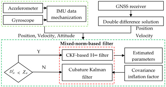
Figure 1.
Flowchart of the mixed norm-based filter applied in the multi-GNSS/IMU integrated systems. After mechanization, the IMU can provide the initial position, velocity and attitude information, and the GNSS can provide the initial position and velocity information. The position and velocity differences between IMU and GNSS are regarded as the measurements input into the filter. Square of the Mahalanobis distance is adopted as the test statistics, and the hypothesis test is implemented at each epoch. If the zero hypothesis is rejected, the CKF is implemented and the covariance inflation factor is applied to control the bad effects of the outlying measurements. Otherwise, the H∞ filter is performed.
4. Experiments and Analysis
The performance of the proposed data fusion algorithm is applied and tested in the data processing of the multi-GNSS/IMU integrated navigation systems. The main equipment of the multi-GNSS/IMU integrated navigation systems consist of two GNSS receivers and an IMU, and the IMU consists of the three-axis accelerometers and the three-axis fiber-optic gyroscope. The GNSS receivers are Trimble R8 geodetic receivers, and they were set to receive the signals of multiple GNSS constellations. One of the receivers was set as the reference station, and another receiver, together with the IMU, was set on the land vehicle to detect its position, velocity, and attitude information. The equipment of these integrated systems is plotted in Figure 2. The nominal RMSE (Root Mean Square Error) for the GNSS receivers and the key technical specifications of the IMU are provided in Table 1.
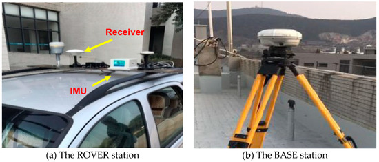
Figure 2.
The basic equipment of the integrated systems.

Table 1.
Key technical specifications of the GNSS receivers and the IMU.
The experiment dataset was collected with the above multi-GNSS/IMU integrated navigation systems. The diagonal elements of the covariance matrix correspond to the errors of the position, and the velocity was set as 0.25 m2 and 0.0025 m2/s2, respectively. According to the technical specifications, the initial position and velocity bias are set to 1.0 m and 0.1 m/s, respectively. After mechanization, the observation information of the IMU and GNSS is constructed and input into the filter. According to the dataset, the motion trajectory and distance of the land vehicle is plotted in Figure 3.
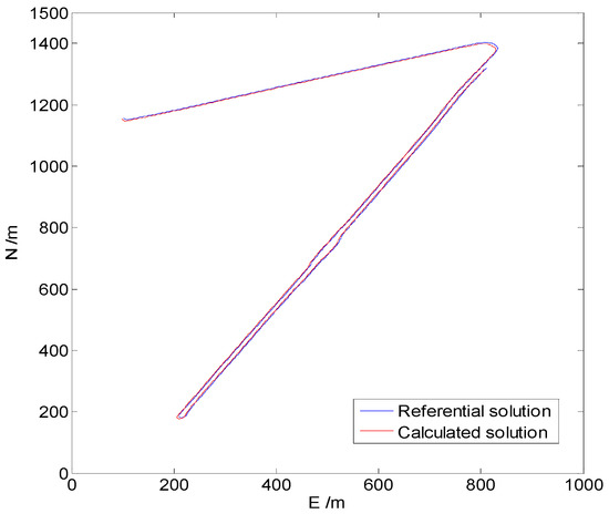
Figure 3.
Motion trajectory and distance of the land vehicle in north and east directions. The trajectory shows that the land vehicle moves in an almost straight direction, except for several turns. The red line denotes the referential solution, and the blue line denotes the solution calculated with self-developed software.
In the experiments, two different cases were designed and organized to compare the performance of different algorithms. Each case consisted of four different algorithms, and these four algorithms were implemented with the same dataset, respectively. The GNSS double-difference carrier phase results calculated from the commercial Inertial Explorer software were adopted as the referential solution, and the results of all four algorithms were compared with the referential solution, respectively. These four algorithms are listed below.
Algorithm 1: the cubature Kalman filter (CKF);
Algorithm 2: the H∞ filter based on the cubature Kalman filter (HF);
Algorithm 3: the mixed norm-based filter with the confidence level of 95% (MC-95);
Algorithm 4: the mixed norm-based filter with the confidence level of 99% (MC-99);
For the H∞ filter of the above algorithms in each case, the threshold parameter was set to 2.
4.1. Case 1
In this case, the four designed algorithms were performed with the initial dataset, respectively. In the filtering process of this paper, the predicted state vector consist of fifteen elements, and the first three elements are the position error variables during the filtering. The values of these three elements of the predicted state vector for different algorithms are plotted in Figure 4, Figure 5, Figure 6 and Figure 7.
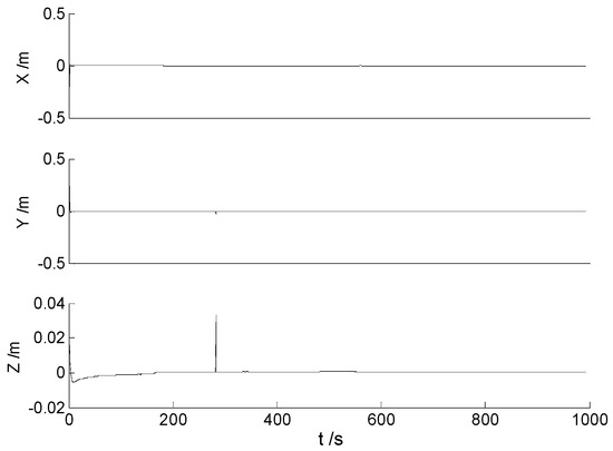
Figure 4.
The position error variables of the predicted state vector for the CKF.
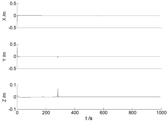
Figure 5.
The position error variables of the predicted state vector for the HF.
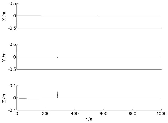
Figure 6.
The position error variables of the predicted state vector for the MC-95.
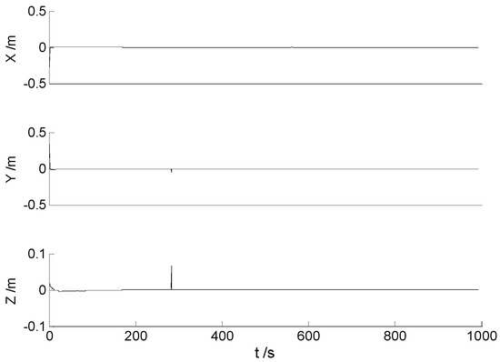
Figure 7.
The position error variables of the predicted state vector for the MC-99.
Figure 4, Figure 5, Figure 6 and Figure 7 demonstrate the position error variables of the predicted state vector for different algorithms. It is found from the above figures that the values of these variables are quite small. However, these are just the process variables, and can hardly demonstrate the performance of different algorithms. Since the final position errors (namely, the differences between the referential solution and the calculated solution) are easier to demonstrate the differences of these algorithms, they are plotted to distinguish the performance of different algorithms. Then, the differences from the referential solution of different algorithms are demonstrated in Figure 8, Figure 9, Figure 10 and Figure 11.
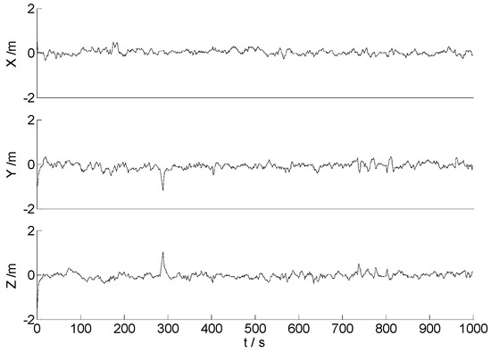
Figure 8.
Position errors of the CKF.

Figure 9.
Position errors of the HF.
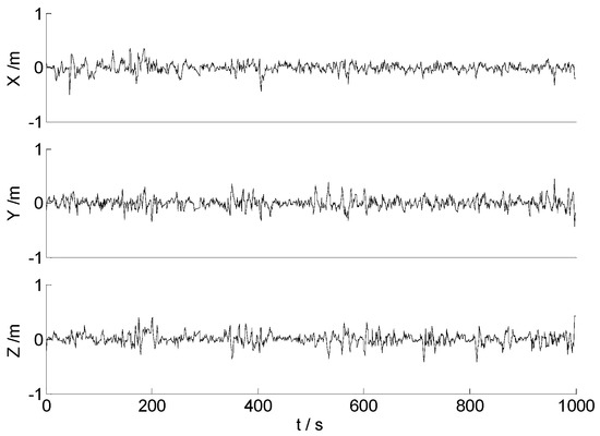
Figure 10.
Position errors of the MC-95.
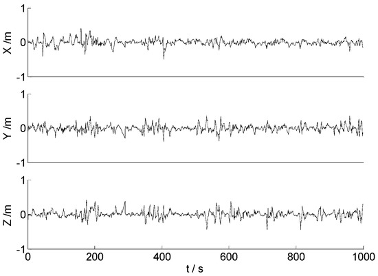
Figure 11.
Position errors of the MC-99.
As the land vehicle travels on the urban road, the complex environment may bring some unpredictable influences to the signals, such as the shelter, the electromagnetic interference, and other uncertain noises. When the land vehicle travels over the speed bumps, the equipped sensors generate an abnormal vibration. This results in some apparent disturbances, as demonstrated in Figure 8. Therefore, the apparent disturbance indicates that the CKF algorithm is sensitive to the abnormal measurements, and the ability of robustness for the CKF algorithm should be enhanced further. Compared with the CKF algorithm, the performance of the HF algorithm plotted in Figure 9 manifests an apparent ability of robustness. Since the dataset contains little disturbances, the null hypothesis is accepted at most epochs, and performance of the algorithms 2–4 is mainly determined by the H∞ filter. Accordingly, in Figure 9, Figure 10 and Figure 11, the positioning errors of different algorithms are similar, since the process of the H∞ filter is relatively stable. In practical applications, the position of the carrier, together with its velocity and attitude, are important parameters to help to make decisions. Therefore, the RMSE of the position (Px, PY, Pz), the velocity (Vx, VY, Vz) and the attitude (Pitch, Yaw) for different algorithms are adopted to depict their performance quantificationally, and the statistical information is presented in Table 2.

Table 2.
RMSE of different algorithms in Case 1.
Table 2 demonstrates that the RMSE values of the CKF algorithm are bigger than those of the other algorithms, especially the RMSE values of the velocity and the attitude. This indicates that the performance of the CKF algorithm is improved by the H∞ filter, since the uncertain noises were well controlled. Compared with the HF algorithm, the MC-95 and MC-99 algorithms performed better with the relatively smaller RMSE values. In fact, for the MC-95 and MC-99 algorithms, the influences of the abnormal measurements were weakened, and the IMU measurements became more accurate after the closed-loop feedback. Compared with the MC-95 algorithm, the null hypothesis was rejected at more epochs in the MC-99 algorithm. More measurements were detected and identified as abnormal, and the weights of these measurements were degraded in the filtering. Therefore, the parameters estimated through the multi-GNSS/IMU integrated navigation systems are more likely to be precise and reliable.
4.2. Case 2
In this case, some significant outliers (40 m) were artificially added into the initial GNSS measurements; thus, the second dataset was constructed. Then, the four designed algorithms were implemented with the second dataset, respectively. Similarly, the position differences from the referential solution are demonstrated in Figure 12, Figure 13, Figure 14 and Figure 15, respectively.
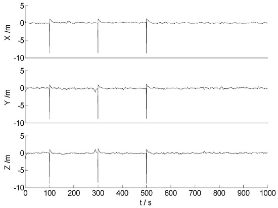
Figure 12.
Position errors of the CKF.
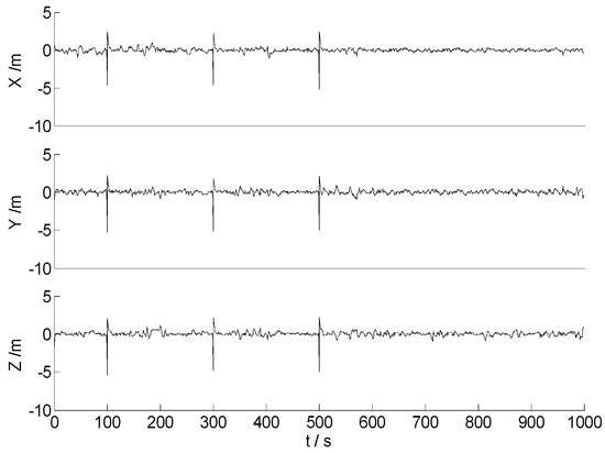
Figure 13.
Position errors of the HF.
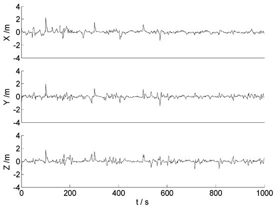
Figure 14.
Position errors of the MC-95.
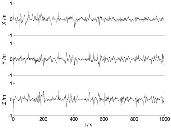
Figure 15.
Position errors of the MC-99.
In Figure 12 and Figure 13, it is demonstrated that both the CKF and the HF algorithms are seriously affected by the significant outliers. Compared with the CKF algorithm, the HF algorithm exerts stronger robustness, and the influences of the significant outliers are weakened further. For the algorithms with mixed norms, the amplitudes of the position errors become much smaller, and no apparent outlying value is found in Figure 14 and Figure 15. This indicates that the effects of the outlying measurements are controlled effectively. In contrast to the MC-95 algorithm, the MC-99 algorithm performs the hypothesis test with a smaller quantile, and more outlying measurements are detected and identified. Therefore, the MC-99 algorithm performs better with the relatively smaller error amplitudes, and the filtering become more stable. It is worth noticing that the threshold should not be too small, as the data utilization efficiency is decreased with an unreasonably small threshold, and the precision of the filtering may become inferior under this scenario. Therefore, the reasonable threshold should be set according to the practical applications. Then, the corresponding statistical information is provided in Table 3.

Table 3.
RMSE of different algorithms in Case 2.
In this case, the influences of the significant outlying measurements become the main factor that affects the precision of the estimates, and it is suitable to test the robustness of different algorithms. In Table 3, the RMSE values indicate that the precision of different algorithms are degraded by the significant outliers, and the RMSE values of the CKF and HF algorithms are several times bigger than those in Case 1, respectively. In terms of the errors of the position, the velocity and the attitude, influences to the velocity and the attitude of the significant outliers are lighter than those in the position. RMSE values of both the MC-95 and MC-99 algorithms are much smaller than those of the CKF and HF algorithms, since the advantages of the H∞ filter and the robust estimation method are combined in the mixed norm-based filtering. Comparing the CKF and the mixed norm-based algorithms, it is demonstrated that the precision of the velocity and the attitude are improved with the mixed norm-based algorithms. For the MC-95 algorithm, considering Table 2 and Table 3, it can be summarized that it is more likely to achieve a better attitude estimation precision with the mixed norm-based algorithms. In this case, the outlying measurement often has an affect not only at the current epoch, but also at the following several epochs. Namely, the significant outliers may cause some new outliers, and the influences at the following epochs usually become lighter than the initial significant outliers. In the hypothesis test, the smaller the threshold, the more outliers can be detected and identified, and the influences of the outliers can be weakened further with the smaller to some extent. Consequently, the MC-99 algorithm performed better than the MC-95 algorithm in this case. Moreover, along with the development of the intelligent PNT (Positioning, Navigation and Timing), more sensors and other available information are integrated and applied in the vehicle positioning, such as the camera [35], the high definition map [36], the laser radar [37], et al. The integration of multiple sensors combines the advantages of different sensors, but the data fusion should always be addressed carefully. Meanwhile, as these above two cases have demonstrated, the proposed data fusion algorithm provides another way to improve the performance of the multi-sensor integration systems, and it can provide some useful references in the practical applications of the parameter estimation.
5. Conclusions
For the data fusion algorithm of the multi-GNSS/IMU integrated navigation systems, the conventional filtering algorithm and most improved algorithms are developed under a single certain norm. In this paper, a different way to improve the performance of the filtering is explored, and a new multi-GNSS/IMU data fusion algorithm with mixed norms is proposed. In the proposed algorithm, the hypothesis test statistics are constructed based on the chi-square distribution to distinguish different scenarios, and the filtering algorithm under different norms is implemented according to different scenarios. The detailed conclusions summarized from the experiments of this paper are listed below.
- (1)
- Compared with the conventional cubature Kalman filter, the H∞ filter manifests a better ability of robustness, since the influences of the uncertain noises are controlled effectively, and the precision of the estimated parameters are improved. However, the performance of the cubature Kalman filter and the H∞ filter is affected significantly by the outlying measurements.
- (2)
- Besides the filtering algorithms, collecting a valid and stable dataset is still an important way to achieve a better filtering solution. A relatively higher precision of the velocity and the attitude estimated in the multi-GNSS/IMU integrated navigation systems is achieved with the H∞ filter, regardless of the existence of some outlying measurements.
- (3)
- By integrating the advantages of the robust estimation and different filtering algorithms, a better performance is achieved with the mixed norm-based algorithms. In this paper, the results of these experiments indicate that it is more likely to achieve a better attitude estimation precision with the mixed norm-based algorithms, but a reasonable threshold for the hypothesis test should be set according to the detailed applications.
- (4)
- In this paper, the cubature Kalman filter and the H∞ filter are selected to construct the mixed norm-based parameter estimation algorithms. Therefore, it is still an open issue to construct different algorithms with different norms, and can provide another way to improve the filtering performance in practical data processing applications.
Author Contributions
C.J. put forward the algorithm, designed the experiments methods, and prepared this manuscript; D.Z. and Q.Z. helped to discuss the experimental results; and W.L. reviewed the whole manuscript. All authors have read and agreed to submit the manuscript.
Funding
This research was partially supported by the Pre-research Project of Songshan Laboratory (YYJC062022013) and the Natural Science Foundation of Henan Province (212300410198).
Data Availability Statement
The data supporting the results in this paper can be obtained through the email jcddtg@163.com.
Conflicts of Interest
The authors declare no conflict of interest.
References
- Yang, Y.X.; He, H.B.; Xu, T.H. Adaptive robust filtering for kinematic GPS positioning. Acta Geod. Et Cartogr. Sin. 2001, 30, 293–298. [Google Scholar]
- Godha, S.; Cannon, M.E. GPS/MEMS INS integrated system for navigation in urban areas. GPS Solut. 2007, 11, 193–203. [Google Scholar] [CrossRef]
- Yang, Y.; Xu, J. GNSS receiver autonomous integrity monitoring (RAIM) algorithm based on robust estimation. Geod. Geodyn. 2016, 7, 117–123. [Google Scholar] [CrossRef]
- Cui, B.; Chen, X.; Tang, X. Improved cubature Kalman filter for GNSS/INS based on transformation of posterior sigma-points error. IEEE Trans. Signal Process. 2017, 65, 2975–2987. [Google Scholar] [CrossRef]
- Jiang, W.; Liu, D.; Cai, B.; Rizos, C.; Wang, J.; Shangguan, W. A Fault-Tolerant Tightly Coupled GNSS/INS/OVS Integration Vehicle Navigation System Based on an FDP Algorithm. IEEE Trans. Veh. Technol. 2019, 68, 6365–6378. [Google Scholar] [CrossRef]
- Chiang, K.; Tsai, G.; Chang, H.; Joly, C.; EI-Sheimy, N. Seamless navigation and mapping using an INS/GNSS/grid-based SLAM semi-tightly coupled integration scheme. Inf. Fusion 2019, 50, 181–196. [Google Scholar] [CrossRef]
- Doostdar, P.; Keighobadi, J.; Hamed, M.A. INS/GNSS integration using recurrent fuzzy wavelet neural networks. GPS Solut. 2020, 24, 1–15. [Google Scholar] [CrossRef]
- Kalman, R.E. A new approach to linear filtering and prediction problems. J. Basic Eng. 1960, 82, 35–45. [Google Scholar] [CrossRef]
- Zhong, M.Y.; Guo JYang, Z.H. On real time performance evaluation of the inertial sensors for INS/GPS integrated systems. IEEE Sens. J. 2016, 16, 6652–6661. [Google Scholar] [CrossRef]
- Ma, C.; Pan, S.; Gao, W.; Ye, F.; Liu, L.; Wang, H. Improving GNSS/INS Tightly Coupled Positioning by Using BDS-3 Four-Frequency Observations in Urban Environments. Remote Sens. 2022, 14, 615. [Google Scholar] [CrossRef]
- Majidi, M.; Erfanian, A.; Khaloozadeh, H. Prediction-discrepancy based on innovative particle filter for estimating UAV true position in the presence of the GPS spoofing attacks. IET Radar Sonar Navig. 2020, 14, 887–897. [Google Scholar] [CrossRef]
- Impraimakis, M.; Smyth, A.W. An unscented Kalman filter method for real time input-parameter-state estimation. Mech. Syst. Signal Process. 2022, 162, 108026. [Google Scholar] [CrossRef]
- Zhao, Y.W. Performance evaluation of cubature Kalman filter in a GPS/IMU tightly-coupled navigation system. Signal Process. 2016, 119, 67–79. [Google Scholar] [CrossRef]
- Arasaratnam, I.; Haykin, S.; Hurd, T.R. Cubature Kalman filtering for continuous-discrete systems: Theory and simulations. IEEE Trans. Signal Process. 2010, 58, 4977–4993. [Google Scholar] [CrossRef]
- Amini Tehrani, H.; Bakhshi, A.; Yang, T.Y. Online jointly estimation of hysteretic structures using the combination of central difference Kalman filter and Robbins–Monro technique. J. Vib. Control. 2021, 27, 234–247. [Google Scholar] [CrossRef]
- Almas, M.A.; Sharma, K. A two stage mean and iterative median filter approach for image denoising. Int. J. Adv. Sci. Technol. 2020, 29, 5355–5361. [Google Scholar]
- Teunissen, P.J.G. Quality control in integrated navigation systems. In Proceedings of the 1990’-A Decade of Excellence in the Navigation Sciences, IEEE PLANS’90 Position Location and Navigation Symposium, Las Vegas, NV, USA, 20 March 1990; pp. 158–165. [Google Scholar]
- Chang, G. Robust Kalman filtering based on Mahalanobis distance as outlier judging criterion. J. Geod. 2014, 88, 391–401. [Google Scholar] [CrossRef]
- Mohamed, A.H.; Schwarz, K.P. Adaptive Kalman filtering for INS/GPS. J. Geod. 1999, 73, 193–203. [Google Scholar] [CrossRef]
- Yang, Y.X.; Ren, X.; Xu, Y. Main progress of adaptively robust filter with applications in navigation. J. Navig. Position. 2013, 1, 9–15. [Google Scholar]
- Xu, Y.; Ahn, C.K.; Shmaliy, Y.S.; Chen, X.; Li, Y. Adaptive robust INS/UWB-integrated human tracking using UFIR filter bank. Measurement 2018, 123, 1–7. [Google Scholar] [CrossRef]
- Fu, Z.; Han, Y. Centroid weighted Kalman filter for visual object tracking. Measurement 2012, 45, 650–655. [Google Scholar] [CrossRef]
- Rigatos, G.; Siano, P.; Wira, P.; Busawon, K.; Binns, R. A nonlinear H-infinity control approach for autonomous truck and trailer systems. Unmanned Syst. 2020, 8, 49–69. [Google Scholar] [CrossRef]
- Gustafsson, F. Particle filter theory and practice with positioning applications. IEEE Aerosp. Electron. Syst. Mag. 2010, 25, 53–82. [Google Scholar] [CrossRef]
- Doucet, A.; Godsill, S.; Andrieu, C. On sequential Monte Carlo sampling methods for Bayesian filtering. Stat. Comput. 2000, 10, 197–208. [Google Scholar] [CrossRef]
- Sun, W.; Liu, J.Z. Cooperative navigation method based on the Huber robust cubature fission particle filter. Chin. J. Sci. Instrum. 2022, 43, 166–175. [Google Scholar]
- Aslan, M.F.; Durdu, A.; Sabanci, K.; Mutluer, M.A. CNN and HOG based comparison study for complete occlusion handling in human tracking. Measurement 2020, 158, 107704. [Google Scholar] [CrossRef]
- Xia, X.; Hashemi, E.; Xiong, L.; Khajepour, A. Autonomous Vehicle Kinematics and Dynamics Synthesis for Sideslip Angle Estimation Based on Consensus Kalman Filter. IEEE Trans. Control. Syst. Technol. 2022, 31, 179–192. [Google Scholar] [CrossRef]
- Liu, W.; Xia, X.; Xiong, L.; Lu, Y.; Gao, L.; Yu, Z. Automated Vehicle Sideslip Angle Estimation Considering Signal Measurement Characteristic. IEEE Sens. J. 2021, 21, 21675–21687. [Google Scholar] [CrossRef]
- Xia, X.; Xiong, L.; Huang, Y.; Lu, Y.; Gao, L.; Xu, N.; Yu, Z. Estimation on IMU yaw misalignment by fusing information of automotive onboard sensors. Mech. Syst. Signal Process. 2021, 162, 107993. [Google Scholar] [CrossRef]
- Gao, L.; Xiong, L.; Xia, X.; Lu, Y.; Yu, Z.; Khajepour, A. Improved Vehicle Localization Using On-Board Sensors and Vehicle Lateral Velocity. IEEE Sens. J. 2022, 22, 6818–6831. [Google Scholar] [CrossRef]
- Zhang, F.X.; Yu, X.R.; He, W.F.; Li, C. Face recognition with improved loss function and multiple norm. Comput. Eng. Appl. 2020, 56, 144–150. [Google Scholar]
- Izenman, A.J. Modern Multivariate Statistical Techniques: Regression, Classification, and Manifold Learning; Springer: New York, NY, USA, 2008. [Google Scholar]
- Yang, Y.; He, H.; Xu, G. Adaptively robust filtering for kinematic geodetic positioning. J. Geod. 2001, 75, 109–116. [Google Scholar] [CrossRef]
- Liu, W.; Xiong, L.; Xia, X.; Lu, Y.; Gao, L.; Song, S. Vision-aided intelligent vehicle sideslip angle estimation based on a dynamic model. IET Intell. Transp. Syst. 2020, 14, 1183–1189. [Google Scholar] [CrossRef]
- Xia, X.; Meng, Z.; Han, X.; Li, H.; Tsukiji, T.; Xu, R.; Zhang, Z.; Ma, J. Automated Driving Systems Data Acquisition and Processing Platform. arXiv 2022, arXiv:2211.13425. [Google Scholar]
- Liu, W.; Quijano, K.; Crawford, M.M. YOLOv5-Tassel: Detecting tassels in RGB UAV imagery with improved YOLOv5 based on transfer learning. IEEE J. Sel. Top. Appl. Earth Obs. Remote Sens. 2022, 15, 8085–8094. [Google Scholar] [CrossRef]
Disclaimer/Publisher’s Note: The statements, opinions and data contained in all publications are solely those of the individual author(s) and contributor(s) and not of MDPI and/or the editor(s). MDPI and/or the editor(s) disclaim responsibility for any injury to people or property resulting from any ideas, methods, instructions or products referred to in the content. |
© 2023 by the authors. Licensee MDPI, Basel, Switzerland. This article is an open access article distributed under the terms and conditions of the Creative Commons Attribution (CC BY) license (https://creativecommons.org/licenses/by/4.0/).