An Improved Backward Smoothing Method Based on Label Iterative Processing

Abstract

Effective target detection and tracking has always been a research hotspot in the field of radar, and multi-target tracking is the focus of radar target tracking at present. In order to effectively deal with the issue of outlier removal and track initiation determination in the process of multi-target tracking, this paper proposes an improved backward smoothing method based on label iterative processing. This method corrects the loophole in the original backward smoothing method, which can cause estimated target values to be erroneously removed due to missing detection, so that it correctly removes outliers in target tracking. In addition, the proposed method also combines label iterative processing with track initiation determination to effectively eliminate invalid target short-lived tracks. The results of simulation experiments and actual data verification showed that the proposed method correctly removed outliers and invalid short-lived tracks. Compared with the original method, it improved the accuracy of target cardinality estimation and tracking performance to a certain extent. Moreover, without affecting the algorithm performance, the method’s processing efficiency could be improved by increasing the track pruning threshold. Finally, the proposed method was compared with existing methods, verifying that its tracking performance was better than that of existing methods.

1. Introduction

Most radar targets are non-cooperative, numbers of targets vary, and the measurements obtained may be missing detection or false alarms, which bring considerable difficulties to detection and tracking. False alarms, missing detection (or a Doppler blind area), and other problems in radar target detection will lead to target track breaking and false target/outlier interference during tracking. Moreover, with the continuous increase in low, small, and slow targets such as floating balloons, it is becoming more and more difficult for existing radar to detect targets [1]. Such targets have weak backscattering of radar-transmitted electromagnetic waves, leading to a significant reduction in the signal-to-noise ratio of signals obtained by radar, which greatly reduce the detection performance of radar. The simultaneous departure of multiple aircraft also tests the radar’s multi-target tracking ability. In addition, in terms of the multi-target tracking problem under different radar systems, for example, the existence of a Doppler blind zone (DBZ) increases the complexity of the multi-target tracking process with Doppler radar, and the resulting continuous missing detection will seriously deteriorate the radar’s multi-target tracking performance. Therefore, effectively achieving multi-target tracking in such a complex scene has always been a research challenge [2].

For the multi-target tracking problem in complex scenes, methods based on RFS theory model the state and measurement of the target as a random finite set that represents the target’s status, such as birth, survival, and extinction, corresponding to the measurement status, such as detection, false alarms, and missing detection. Therefore, this became a research hotspot once proposed. RFS-based tracking methods include the Probability Hypothesis Density (PHD) filter [3], Cardinalized PHD (CPHD) filter [4], Cardinality–Balanced Multi-Bernoulli (CB-MeMBer) filter [5], Generalized Labeled Multi-Bernoulli (GLMB) filter [6], Labeled Multi-Bernoulli (LMB) filter [7], etc. In particular, the LMB filter can efficiently output the continuous track of the target, which has great application value. Therefore, this paper took the LMB filter as the core of the processing algorithm.

In order to further improve tracking accuracy, researchers introduced smoothing, which utilize all measurements at the current time to correct the target’s state in the past. With the introduction of RFS/Labeled-RFS theory, the application efficiency of smoothing processing has been further improved. The authors of [8] proposed a Bernoulli smoother that had significantly better tracking performance than the Bernoulli filter and was an accurate tracking smoother, but it was only suitable for tracking problems with no more than one target. For multi-target tracking problems, the authors of [9] proposed a forward–backward PHD smoother, which could improve the accuracy of target location estimation compared to the PHD filter but may not necessarily improve the accuracy of cardinality estimation. The authors of [10] proposed a CPHD smoother that used an approximate structure to overcome the computational complexity of the typical CPHD smoother, which was complex and difficult to implement. The authors of [11] proposed a multi-Bernoulli (MB) smoother with a backward smoothing step similar to an update step. The MB smoother had the problem of early target extinction, where the estimated extinction time was earlier than the actual extinction time of the target. However, the smoothers and corresponding filters mentioned above did not consider the target’s label and did not provide track information corresponding to the target.

Subsequently, multi-target trackers based on Labeled-RFS theory, represented by the LMB and GLMB filters, could efficiently output continuous tracks of targets and have significant application value. The authors of [12] proposed a GLMB smoother, which was the first exact closed form solution for the Labeled-RFS smoothing algorithm. However, its data association was very complex and not easy to implement. The authors of [13] proposed a multi-frame GLMB filter, which had a structure of simultaneous filtering and smoothing. Previous experiments have shown that its performance was better than that of other filters. However, in order to reduce the computational complexity, an NP hard multidimensional assignment problem needed to be solved during implementation. Even if the Gibbs sampling method was used, the computational complexity of the method was still significant.

The authors of [14] proposed a one-step lagged δ-GLMB smoother, which was superior to the δ- GLMB filter and CPHD smoother with the same delay in target cardinality and state estimation, and it was also superior to the LMB smoother and an approximate δ- GLMB smoother with the same delay in target cardinality estimation. Under the pulse Doppler radar system, the authors of [15] proposed the sequential Monte Carlo implementation form of the forward–backward LMB smoother based on the forward–backward LMB smoother proposed in [16], and through theoretical derivation and numerical analysis it was found that the proposed LMB smoother could improve the accuracy of target cardinality and state estimations and the main computational complexity was linear with the number of targets. Finally, the effectiveness and computational efficiency of the proposed smoother was verified through experiments. The authors of [17] provided a detailed comparison of the tracking performance of the forward–backward LMB smoother mentioned above with that of the LMB filter, PHD filter, PHD smoother, CB-MeMBer filter, and MB smoother, further verifying its effectiveness. The authors of [18] took pulse Doppler radar as the application scenario, and for actual data processing, the forward–backward LMB smoother based on label iterative processing was used to eliminate filtered outliers during the tracking process and output smooth estimated tracks to improve tracking accuracy. In addition, continuity judgment of tracks and effective track extraction were introduced to eliminate false tracks and obtain the final output track. However, during the research process, it was found that this method had problems that led to erroneous removal of target estimation points due to missing detection of the target and was accompanied by a certain length of track breakage formed by the backward smoothing step, thereby reducing the overall target tracking performance.

In the process of multi-target tracking, state and track estimations are processed to improve tracking performance. In the existing research algorithms, most rely on certain track management strategies to achieve the purpose of track processing, such as in [18,19], and are usually managed and processed in the form of batch processing, which makes the algorithm lose the possibility of real-time processing. The Labeled-RFS-based method includes processing of the target’s birth, survival, and death. There is no need to consider the problem of target track management (data association, track initiation, maintenance, and termination) as with the traditional method during individual processing. Due to the introduction of labels, the radar multi-target tracking algorithm based on Labeled-RFS theory can realize track processing and management more effectively through label iterative processing to achieve high performance. Therefore, exploring label iterative processing is a feasible way to realize the sequential processing of tracks.

This paper takes the tracking issue of typical unmanned aerial vehicle targets under the pulse Doppler (PD) radar system as the research background. In order to optimize the false alarm/outlier processing and invalid short-lived problem in radar multi-target tracking, an improved backward smoothing method (improved method: I-BS smoother) is proposed based on the LMB filter. The advantages of this method lie in: (1) correcting the problem of the original backward smoothing method (original method: O-BS smoother) in [18], so that it is not affected by missing detection, can correctly remove outliers, and output smoothing estimation tracks; (2) integrating the label iteration processing with track initiation determination to sequentially process invalid short-lived tracks; and (3) the proposed algorithm can ensure algorithm performance while reducing the computational burden of real-time processing by reducing the track pruning threshold. Figure 1 shows the processing flowchart and novelties of the proposed method, with the improvements marked in the red box. Finally, this paper verifies the effectiveness of the proposed algorithm in removing outliers and invalid short-lived tracks through simulation experiments and measured data validation. Compared with the original method, the accuracy of target cardinality and state estimations was improved to a certain extent, and the processing efficiency of the algorithm was further improved due to the reduction of the track pruning threshold. Finally, this paper compares the proposed method with the forward–backward LMB smoother [17] and the One Time Step Lagged δ-GLMB smoother [14] under the same experimental conditions to verify that the proposed method has better tracking performance than existing methods.

The rest of this article is organized as follows. Section 2 first briefly introduces the theoretical background of the proposed method—the LMB filter. In Section 3, the theoretical derivation of the proposed smoother is given. Section 4 presents the simulation and experimental results to verify the effectiveness of the proposed method. Section 5 introduces the conclusion of the paper and future research expectations.

2. LMB Filters

The labeled multi-target state can be expressed as $\mathrm{X}=\{{\mathrm{x}}_1,\cdots ,{\mathrm{x}}_i,\cdots ,{\mathrm{x}}_{\left|\mathrm{X}\right|}\}$, where ${\mathrm{x}}_i=(x_i,{{\displaystyle \mathit{\ell }}}_i)$ is the labeled single-target state, ${\mathit{\ell }}_i$ is the label of target $x_i$, $\left|\mathrm{X}\right|$ is the cardinality (or the number of targets) of the multi-target state, $\mathrm{X}\subset X\times L$, and $X$ and $L$ are the state and label spaces, respectively.

If $\mathrm{X}$ obeys the LMB distribution [7], its density function can be expressed as:

$$\pi (\mathrm{X})=\Delta (\mathrm{X})\omega (L(\mathrm{X}))p^{\mathrm{X}}$$

(1)

where mapping $L:X\times L\to L$ makes $L(x,\mathit{\ell })=\mathit{\ell }$, $L(\mathrm{X})=\{\mathit{\ell }:(x,\mathit{\ell })\in \mathrm{X}\}$. $\Delta (\mathrm{X})={\delta }_{\left|\mathrm{X}\right|}(\left|L(\mathrm{X})\right|)$ is defined as indicator functions of different labels: when the labels in $\mathrm{X}$ are different, $\Delta (\mathrm{X})=1$; If $\mathrm{X}\ne \varnothing$, then $p^{\mathrm{X}}={\displaystyle {\prod }_{x\in X}p(x,\mathit{\ell })}$, $p(x,\mathit{\ell })$ are the probability density functions of the target. If $\mathrm{X}=\varnothing$, then $p^{\mathrm{X}}=1$.

Assume that the weight $\omega (L(\mathrm{X}))$ can be expressed as:

$$\omega (L(\mathrm{X}))={\displaystyle \prod _{\mathit{\ell }\in L}(1-r^{\mathit{\ell }})}{\displaystyle \prod _{\mathit{\ell }\in L(\mathrm{X})}\frac{1_L(\mathit{\ell })r^{\mathit{\ell }}}{1-r^{\mathit{\ell }}}}$$

(2)

where $1_L(\mathit{\ell })$ is the containing function when $\mathit{\ell }\in L$, $1_L(\mathit{\ell })=1$, otherwise, it is equal to 0. $r^{\mathit{\ell }}$ is the probability of existence of target $x$ marked with $\mathit{\ell }$, $\mathit{\ell }\in L$. The equivalent parameter form of the LMB distribution density function can be expressed as:

$$\pi ={\{(r^{\mathit{\ell }},p^{\mathit{\ell }})\}}_{l\in L}$$

(3)

The LMB smoothing filter consists of forward filtering and backward smoothing. The forward filtering adopts the standard LMB filter [20], which also includes the prediction and update process. Therefore, the LMB smoothing filter consists of prediction, update, and backward smoothing, and the standard LMB filter is described below.

2.1. Predict

Suppose that the probability density of multiple targets at time $t-1$ follows the LMB distribution, expressed as ${\pi }_{t-1\left|t-1\right.}={\{(r_{t-1\left|t-1\right.}^{\mathit{\ell }},p_{t-1\left|t-1\right.}^{\mathit{\ell }})\}}_{\mathit{\ell }\in L}$. The newborn target also obeys the LMB distribution, expressed as ${\pi }_{B,t}={\{(r_{B,t}^{\mathit{\ell }},p_{B,t}^{\mathit{\ell }})\}}_{\mathit{\ell }\in B}$, and the total label set is expressed as $L_{+}=L\cup B$, so the prediction probability density can be expressed as [20]:

$${\pi }_{t\left|t-1\right.}={\{(r_{t\left|t-1\right.}^{\mathit{\ell }},p_{t\left|t-1\right.}^{\mathit{\ell }})\}}_{\mathit{\ell }\in L_{+}}={\{(r_{B,t}^{\mathit{\ell }},p_{B,t}^{\mathit{\ell }})\}}_{\mathit{\ell }\in B}\cup {\{(r_{s,t\left|t-1\right.}^{\mathit{\ell }},p_{s,t\left|t-1\right.}^{\mathit{\ell }})\}}_{\mathit{\ell }\in L}$$

(4)

where

$$r_{s,t|t-1}^{\mathit{\ell }}={\eta }_{s,t|t-1}^{\mathit{\ell }}{r}_{t-1|t-1}^{\mathit{\ell }}$$

(5)

$${\eta }_{s,t|t-1}^{\mathit{\ell }}=〈p_{s,t\left|t-1\right.}^{\mathit{\ell }}(\cdot ),p_{t-1\left|t-1\right.}^{\mathit{\ell }}(\cdot )〉$$

(6)

$$p_{s,t\left|t-1\right.}^{\mathit{\ell }}=\frac{〈p_{s,t\left|t-1\right.}(\cdot ,\mathit{\ell })f_{t\left|t-1\right.}(x_{+}|(\cdot ,\mathit{\ell })),p_{t-1\left|t-1\right.}^{\mathit{\ell }}(\cdot ,\mathit{\ell })〉}{{\eta }_{s,t|t-1}^{\mathit{\ell }}}$$

(7)

$$p_{t\left|t-1\right.}^{\mathit{\ell }}(x_{+},\mathit{\ell })=1_L(\mathit{\ell })p_{s,t\left|t-1\right.}^{\mathit{\ell }}(x_{+},\mathit{\ell })+1_B(\mathit{\ell })p_{B,t}^{\mathit{\ell }}(x_{+},\mathit{\ell })$$

(8)

where $f_{t\left|t-1\right.}(x_{+}|(\cdot ,\mathit{\ell }))$ is the Markov transfer density of target $x$, and $p_{s,t\left|t-1\right.}(\cdot ,\mathit{\ell })$ is the survival probability of target $x$. $“+”$ represents the current time $t$.

2.2. Update

Suppose that the probability density function of the prediction step at time $t$ follows the LMB distribution, which can be expressed as:

$${\pi }_{t\left|t-1\right.}={\{(r_{t\left|t-1\right.}^{\mathit{\ell }},p_{t\left|t-1\right.}^{\mathit{\ell }})\}}_{\mathit{\ell }\in L_{+}}=\Delta ({\rm X}){\omega }_{t\left|t-1\right.}(L({\rm X})){[p_{t\left|t-1\right.}^{\mathit{\ell }}]}^{{\rm X}}$$

(9)

At this time, the multiple objective posterior probability density function at time $t$ obeys the GLMB distribution [18], and the specific form is given by:

$${\pi }_{t\left|t\right.}=\Delta ({\rm X})\cdot {\displaystyle \sum _{(I_{+},\theta )\in F(L_{+})\times {\Theta }_{I_{+}}}{\omega }_{t\left|t\right.}^{(I_{+},\theta )}(Z){\delta }_{I_{+}}\left(L\left({\rm X}\right)\right){[p_{t\left|t\right.}^{\theta }\left(x,\mathit{\ell }\right)]}^{{\rm X}}}$$

(10)

where

$${\omega }_{t\left|t\right.}^{(I_{+},\theta )}\propto {\omega }_{t|t-1}(I_{+}){[{\eta }_Z^{\theta }]}^{I_{+}}$$

(11)

$$p_{t\left|t\right.}^{\theta }(x,\mathit{\ell })=\frac{p_{t|t-1}(x,\mathit{\ell })\cdot {\psi }_Z(x,\mathit{\ell };\theta )}{{\eta }_Z^{\theta }(\mathit{\ell })}$$

(12)

$${\eta }_Z^{\theta }(\mathit{\ell })=〈p_{t|t-1}(\cdot ,\mathit{\ell }),{\psi }_Z( ,\mathit{\ell };\theta )〉$$

(13)

$${\psi }_Z(x,\mathit{\ell };\theta )=\left\{\begin{array}{l}\frac{p_D(x,\mathit{\ell }) \cdot g(z_{\theta \left(\mathit{\ell }\right)}|x,\mathit{\ell })}{\kappa (z_{\theta \left(\mathit{\ell }\right)})} ,\theta (\mathit{\ell })>0\\ 1-p_D(x,\mathit{\ell }) , \theta (\mathit{\ell })=0\end{array}\right.$$

(14)

where $I_{+}=\{{\mathit{\ell }}_1,\dots ,{\mathit{\ell }}_{\left|I_{+}\right|}\}$ is a hypothetical label set. ${\delta }_{\mathrm{Y}}(\mathrm{X})=\left\{\begin{array}{l}1,\mathrm{X}=\mathrm{Y}\\ 0,\mathrm{X}\ne \mathrm{Y}\end{array}\right.$ is the generalized Kronecker Delta function, for which the independent variable ${\delta }_{\mathrm{Y}}(\mathrm{X})$ can take any form, such as set, vector, matrix, etc. ${\Theta }_{I_{+}}$ is a set of mappings $\theta :I_{+}\to \{0,1,\dots ,\left|Z\right|\}$, and when $\theta \left({\mathit{\ell }}_i\right)=\theta \left({\mathit{\ell }}_{i^{\prime }}\right)>0$, ${\mathit{\ell }}_i={\mathit{\ell }}_{i^{\prime }}$; ${\omega }_{t\left|t\right.}^{(I_{+},\theta )}$ is the weight value of hypothesis $(I_{+},\theta )$. $g\left(z_{\theta \left(\mathit{\ell }\right)}|x,\mathit{\ell }\right)$ is the detection probability of the target. $\kappa (\cdot )$ is the density function of clutter. $p_D(x,\mathit{\ell })$ is the detection probability of target $(x,\mathit{\ell })$. If it is approximated by the LMB distribution that is the same as its own first moment, then the posterior density of multiple objects at time t can be approximately written as [19]:

$${\pi }_{t\left|t\right.}\approx {\{(r_{t\left|t\right.}^{\mathit{\ell }},p_{t\left|t\right.}^{\mathit{\ell }}(x,\mathit{\ell }))\}}_{\mathit{\ell }\in L_{+}}$$

(15)

where

$$r_{t\left|t\right.}^{\mathit{\ell }}={\displaystyle \sum _{(I_{+},\theta )\in F(L_{+})\times {\Theta }_{I_{+}}}{\omega }_{t\left|t\right.}^{(I_{+},\theta )}(Z)1_{I_{+}}\left(\mathit{\ell }\right)}$$

(16)

$$p_{t\left|t\right.}^{\mathit{\ell }}\left(x,\mathit{\ell }\right)=\frac{1}{r_{t\left|t\right.}^{\mathit{\ell }}}{\displaystyle \sum _{(I_{+},\theta )\in F(L_{+})\times {\Theta }_{I_{+}}}{\omega }_{t\left|t\right.}^{(I_{+},\theta )}(Z)1_{I_{+}}\left(\mathit{\ell }\right)p_{t\left|t\right.}^{\theta }\left(x,\mathit{\ell }\right)}$$

(17)

3. Improved Backward Smoothing Method Based on Label Iterative Processing

3.1. Improved Backward Smoothing Method

On the basis of the standard LMB filter, this paper introduced backward smoothing to manage and process outliers and tracks, so the LMB filter was improved into the LMB smoothing filter. The LMB smoothing filter was composed of forward filtering and backward smoothing. The forward filtering adopted the standard LMB filter [7], which also included the prediction and update process. The specific derivation was given in Section 2. Therefore, the LMB smoothing filter was composed of prediction, update, and backward smoothing. This paper focused on improving the backward smoothing process. The improved algorithm steps of backward smoothing are given below.

First, the standard backward smoothing process is described. Suppose that the forward filtering reaches time $t$, the backward smoothing density from time $t$ to time $k(k<t)$ is ${\pi }_{k\left|t\right.}(\mathrm{X})$, and the backward smoothing density from time $t$ to time $k-1$ is ${\pi }_{k-1\left|t\right.}(Y)$. It is known from LMB forward filtering that ${\pi }_{k-1\left|k-1\right.}(\mathrm{X})$ and ${\pi }_{k\left|k-1\right.}(\mathrm{X})$ obey the LMB distribution. If ${\pi }_{k\left|t\right.}(\mathrm{X})$ obeys the LMB distribution, ${\pi }_{k-1\left|t\right.}(\mathrm{X})$ still obeys the LMB distribution, and ${\pi }_{k-1\left|t\right.}(\mathrm{X})$ can be expressed as [15,16]:

$${\pi }_{k-1\left|t\right.}={\left\{(r_{k-1\left|t\right.}^{\mathit{\ell }},p_{k-1\left|t\right.}(x,\mathit{\ell }))\right\}}_{l\in L}$$

(18)

where

$$r_{k-1\left|t\right.}^{\mathit{\ell }}=1-\frac{(1-r_{k-1\left|k-1\right.}^{\mathit{\ell }})(1-r_{k\left|t\right.}^{\mathit{\ell }})}{(1-r_{k\left|k-1\right.}^{\mathit{\ell }})}$$

(19)

$$p_{k-1\left|t\right.}^{\mathit{\ell }}(x,\mathit{\ell })=\frac{p_{k-1\left|t\right.}^{\mathit{\ell }}(x,\mathit{\ell })\left({\alpha }_{s,k\left|t\right.}(x,\mathit{\ell })+{\displaystyle \int \frac{{\beta }_{s,k\left|t\right.}(x,\mathit{\ell })f_{k\left|k-1\right.}(y|x,\mathit{\ell })p_{k\left|t\right.}(y,\mathit{\ell })}{p_{k\left|k-1\right.}(y,\mathit{\ell })}dy}\right)}{{\displaystyle \int p_{k-1\left|k-1\right.}(x,\mathit{\ell })\left({\alpha }_{s,k\left|t\right.}(x,\mathit{\ell })+{\displaystyle \int \frac{{\beta }_{s,k\left|t\right.}(x,\mathit{\ell })f_{k\left|k-1\right.}(y|x,\mathit{\ell })p_{k\left|t\right.}(y,\mathit{\ell })}{p_{k\left|k-1\right.}(y,\mathit{\ell })}dy}\right)dx}}$$

(20)

where ${\alpha }_{s,k\left|t\right.}(x,\mathit{\ell })$ and ${\beta }_{s,k\left|t\right.}(x,\mathit{\ell })$ are defined as:

$${\alpha }_{s,k\left|t\right.}(x,\mathit{\ell })=\frac{(1-r_{k\left|t\right.}^{\mathit{\ell }})(1-p_{s,k\left|k-1\right.}(x,\mathit{\ell }))}{(1-r_{k\left|k-1\right.}^{\mathit{\ell }})}$$

(21)

$${\beta }_{s,k\left|t\right.}(x,\mathit{\ell })=\frac{r_{k\left|t\right.}^{\mathit{\ell }}(p_{s,k\left|k-1\right.}(x,\mathit{\ell })}{r_{k\left|k-1\right.}^{\mathit{\ell }}}$$

(22)

In the backward smoothing processing step in [18], in order to eliminate outliers, it only considered the target’s posterior probability density ${\pi }_{k\left|t\right.}\cap {\pi }_{k-1\left|k-1\right.}$ corresponding to label set $L_{k-1\left|t\right.}=L_{persistent}=L_{k\left|t\right.}\cap L_{k-1\left|k-1\right.}$ for processing. That is, it only considered backward smoothing of targets (labels) that existed at time $k$ and $k-1$, and then estimated and outputted the state of the targets. This led to the problem of track fracture due to the target being wrongly deleted when the target was missing.

In order to solve the above problem, this paper proposed an improved backward smoothing processing method integrating the track initiation determination function, which could effectively eliminate outliers and invalid short-lived target tracks at the same time. The detailed steps are as follows.

Step 1: Find out the persistent target label (both at $k$ and $k-1$), and perform backward smoothing filtering:

$$L_{persistent}=L_{k\left|t\right.}\cap L_{k-1\left|k-1\right.}$$

(23)

Then obtain below according to the backward smoothing Equations (18)–(20):

$${\{(r_{k-1\left|t\right.}^{\mathit{\ell }},p_{k-1\left|t\right.}(x,\mathit{\ell }))\}}_{l\in L_{persistent}}$$

(24)

Step 2: Through tracing and statistics on target labels, find out which of these target labels have been wrongly rejected due to missing detection, and eliminate the labels corresponding to outliers and invalid short-lived targets.

First, find the target label set below that vanishes at time $k-1$.

$$L_{death}=setxor(L_{k-1\left|k-1\right.},L_{persistent}=L_{k\left|t\right.}\cap L_{k-1\left|k-1\right.})$$

(25)

where $setxor$ represents the XOR operation.

Then, in the vanishing label set $L_{death}$, we could determine which target labels were outliers and which target labels were wrongly eliminated due to missing detection by the tracing and statistics of the labels. The determination principle is described as follows: for the backward smoothing processing step at time $k-1$, we can count the number of occurrences of each label at $1:t$, and then determine whether the number of occurrences of each label in the vanishing target label set at time $k-1$ exceeds the effective limit $dt$. If it exceeds the limit, it will be determined as the target label that has been wrongly rejected due to missing detection. If it does not exceed the limit, it will be determined as an outlier or invalid short-lived target.

$$L_{missed}=\{{\mathit{\ell }}_i\in L_{death},i=1,\dots ,\left|L_{death}\right| \left|\mathrm{num}\left({\mathit{\ell }}_i\in L_{1:t}\right)>dt\right.\}$$

(26)

where $\mathrm{num}(\cdot )$ is the number of labels in ${\mathit{\ell }}_i=L_{1:t}$.

Step 3: Perform backward smoothing of the output with iterative label processing, eliminate outliers and invalid short-lived tracks, and output the modified processing result.

$$\begin{array}{l}{\pi }_{k-1\left|t\right.}={\left\{(r_{k-1\left|t\right.}^{\mathit{\ell }},p_{k-1\left|t\right.}(x,\mathit{\ell }))\right\}}_{l\in L_{k-1\left|t\right.}}\\ ={\left\{(r_{k-1\left|t\right.}^{\mathit{\ell }},p_{k-1\left|t\right.}(x,\mathit{\ell }))\right\}}_{l\in L_{persistent}}\cdots \\ \cup {\left\{(r_{k-1\left|k-1\right.}^{\mathit{\ell }},p_{k-1\left|k-1\right.}(x,\mathit{\ell }))\right\}}_{l\in L_{missed}}\end{array}$$

(27)

The above processing steps effectively solved the problem brought about in [18] and could also eliminate invalid short-lived tracks, thus improving the target tracking performance. The effectiveness of the proposed method was verified through later experiments.

3.2. State Estimation

After particle resampling, we needed to use clustering technology to extract the multi-target state, that is, to complete multi-target state estimation. The position dimensions of all particles were clustered according to the K-means clustering algorithm [21], with the multi-target state estimation at time $t$ given by:

$${\left\{\right\{({\hat{x}}_{t,1},{\mathit{\ell }}_{t,1})\},\dots ,({\hat{x}}_{t,\left|L_t\right|},{\mathit{\ell }}_{t,\left|L_t\right|})\}}_{\mathit{\ell }\in L_t}$$

(28)

where ${\hat{x}}_{t,i}$ is the $i\mathrm{th}$ target state extracted, ${\mathit{\ell }}_{t,i}$ represents the label of the target state, and $L_t$ is the set of estimated labels corresponding to all estimated target states at time $t$.

3.3. Algorithm Model and Implementation

The algorithm was implemented by sequential Monte Carlo (SMC), namely a particle filter. Since this paper focused on processing at the label level and did not care about the specific implementation form, this paper does not give the specific implementation form of the algorithm, whether it is Gaussian Mixture (GM) [22], Sequential Monte Carlo (SMC) technology/particle filter [23,24], or box particle filter [25]. The specific implementation form can be found in [15]. Readers can refer to the paper’s ideas and apply them to other forms and models.

State transfer equation: This paper considered the discrete acceleration model as the state transfer equation. The state variable of a single target is expressed as ${\mathrm{x}}_t=(x_t,{\mathit{\ell }}_t)$, where ${\mathrm{x}}_t={\left[p_t,{\dot{p}}_t,{\ddot{p}}_t,\right]}^{{\rm T}}$ represents the distance, radial velocity and radial acceleration of the target. The state transfer equation is:

$${\mathrm{x}}_t=F{\mathrm{x}}_{t-1}+G{w}_{t-1}$$

(29)

where $w_{t-1}$ is the state noise of ${\mathrm{x}}_t$, $w_{t-1}~N(w;0,{\sigma }_w^2)$, $F$ is the state transition matrix, and $G$ is the noise transformation matrix.

$$F=\left[\begin{array}{ccc}1& T& \frac{T^2}{2}\\ 0& 1& T\\ 0& 0& 1\end{array}\right]$$

(30)

$$G=\left[\begin{array}{ccc}\frac{T^2}{2}& T& 1\end{array}\right]$$

(31)

The measurement is the distance and speed with noise, and the measurement equation is:

$${\mathrm{z}}_k={\left[r_k,v_k\right]}^{{\rm T}}+{\epsilon }_k$$

(32)

where the measured noise is ${\epsilon }_k~N( \cdot ; 0 , P_{\epsilon })$, $P_{\epsilon }=diag({\sigma }_r^2,{\sigma }_v^2)$.

In this paper, measurement was used to drive the birth. The target tracked in the application was a non-cooperative target, and there was no prior information about the target’s birth position. The measurement was generated by the target or clutter. The target was near the measurement, and the target’s birth information could be inverted by the measurement, which is called measurement-driven birth (or adaptive birth). Suppose that the target birth distribution follows the LMB distribution, and each component of the LMB distribution follows the Gaussian distribution. With reference to [18], the LMB birth distribution of time $t$ is determined by measurement $Z_{t-1}$ of time $t-1$$,$ and each component corresponds to a measurement value of time $t-1$. The target birth distribution can be written as:

$${\pi }_{B,t}={\left\{(r_{B,t}^{\mathit{\ell }}(z),p_{B,t}^{\mathit{\ell }}(x|z))\right\}}_{l\in B}$$

(33)

where $r_{B,t}^{\mathit{\ell }}(z)$ is the birth probability of the newborn target $\mathit{\ell }$ corresponding to measurement $z(z\in Z_{t-1})$, $p_{B,t}^{\mathit{\ell }}(x|z)$ is the corresponding probability density, and $\left|B\right|=\left|Z_{t-1}\right|$ represents the number of hypothetical components. On the one hand, if a measurement has been associated with many assumptions, that is, it has been associated with a living target, it is likely that it will not drive another newborn target because one measurement can only correspond to one target. On the other hand, if a measurement is not included in any hypothesis, it is more likely to drive a newborn target. Therefore, the larger the correlation probability between measurement $z$ and hypothesis $r_{U,t-1}(z)$, the smaller the probability of a measurement-driven target birth. The correlation probability of measurement $z$ is given by:

$$r_{U,t-1}(z)={\displaystyle \sum _{(I,\theta )\in F(L)\times {\theta }_I}{1}_{\theta }(z) }{\omega }_{t-1\left|t-1\right.}^v$$

(34)

where $1_{\theta }(z)$ judges whether a hypothetical weight is associated with measurement $z$. If it is associated, the weight value is added to the association probability. If measurement $z$ is not associated with any hypothesis, then $r_{U,t-1}(z)=0$. The birth probability of the measured corresponding component can be defined as:

$$r_{B,t}^{\mathit{\ell }}(z)=\min (r_{B,\max }(z),\frac{(1-r_{U,t-1}(z){\lambda }_{B,t})}{{\displaystyle \sum _{\xi \in Z_{t-1}}1-r_{U,t-1}(\xi )}}$$

(35)

where $r_{B,\max }$ is the maximum of the set newborn probability and ${\lambda }_{B,t}$ is the expected target birth number at time $t$.

3.4. Evaluation Benchmark

The analysis of the tracking performance of the algorithm in the experiment was mainly carried out from two aspects: tracking accuracy (estimation error) and tracking integrity (cardinality estimation). From the perspective of RFS, the essence of the target tracking algorithm is to measure the difference between finite sets. Therefore, the commonly used multi-target kinematic state evaluation algorithms is the Optimal Sub Pattern Assignment (OSPA) distance [26], which is defined as:

$$d_{p,c}^{Dist}(X,Y)=\left\{\begin{array}{cc}{\left(\underset{\pi \in {\Pi }_n}{\min }\frac{1}{n}{\displaystyle \sum _{i=1}^m{d}^{(c)}{(x_i,y_{\pi (i)})}^p}+\frac{c^p(n-m)}{n}\right)}^{1/p}& ,m\le n\\ d_{p,c}^{Dist}(Y,X)& ,m>n\\ \\ 0& ,m=n=0\end{array}\right.$$

(36)

where $X=\left\{x_1,\cdots ,x_m\right\}$ and $Y=\left\{y_1,\cdots ,y_n\right\}$ are the unlabeled estimated state set and the target real state set, respectively; $m$ and $n$ are the number of these finite non-empty state subsets; ${\Pi }_n$ represents all possible permutations on the set $\left\{1,2,\cdots ,n\right\}$, of which $\pi (i)$ is one of them; $d^{(c)}( \cdot , \cdot )=\min \left(c,‖x-y‖\right)$, with $‖ \cdot ‖$ representing the Euclidean distance and $c$ is the truncation distance. There are two parameters in OSPA, $c$ and $p$. $c$ controls the weight of the cardinality and location errors, where the larger the value of $c$, the stronger the influence of OSPA’s cardinality error. $p$ determines the sensitivity to outliers.

The OSPA distance is composed of the OSPA location and cardinality error components, respectively defined as:

$$d_{p,c}^{Loc}(X,Y)={\left(\underset{\pi \in {\Pi }_n}{\min }\frac{1}{n}{\displaystyle \sum _{i=1}^m{d}^{(c)}{(x_i,y_{\pi (i)})}^p}\right)}^{1/p}$$

(37)

$$d_{p,c}^{Card}(X,Y)=c{\left(\frac{n-m}{n}\right)}^{1/p}$$

(38)

which are used to evaluate the accuracy of location and cardinality estimations, respectively.

4. Experiment Analysis

In this paper, the tracking of typical targets in the pulse Doppler (PD) radar system was taken as the research background, and the effectiveness of the proposed method was verified by simulation and measured data combined with actual background parameters. The

Table 1. Radar parameters.

Parameter	Value	Unit
Carrier frequency	35	GHz
Pulse repetition frequency	32	kHz
Distance sampling interval	1.875	m
Distance sampling points	319	-

gives the basic parameters of the radar.

According to the basic parameters above, the wavelength of the radar was 0.0086 m, the maximum unambiguous speed was 137.14 m/s (the range of unambiguous speed was 0~137.14 m/s), and the maximum unambiguous distance was 4688 m. In order to avoid the impact of speed and distance ambiguity, this paper set the target speed and observation scene width with reference to the above data.

Scene parameter setting: because the method performance of [18] was mainly being compared, the scene setting in this paper and the measured data source were the same as in [18], and the scene setting depended on the measured data parameters. In this paper, the distance range of the actual observation scene was $1.875 \times 319 \approx 598 \mathrm{m}$, and the speed did not exceed $120 \mathrm{m}/\mathrm{s}$. Considering the fluctuation of the gate opening time and retaining some redundancy, the observation area was set to $\left[800,2200\right] \mathrm{m} \times \left[-120,120\right] \mathrm{m}/\mathrm{s}$.

Although this paper mainly considered target tracking, the sampling period $T$ was determined by the pulse accumulation time. When the pulse accumulation time was 800 pulses, $T=0.025 s$. When the pulse accumulation time was 1600 pulses, $T=0.05 s$. Considering the calculation efficiency, this paper adopted a compromise of coherent accumulation time of 25 ms, that is, 800 pulses for coherent accumulation, $T=0.025 s$. Under the condition of accurate focusing, the velocity accuracy could reach 0.086 m/s.

Target motion noise: when $T=0.025 s$, the standard deviation of process noise at each time step could be set as ${\sigma }_w=0.5$, and the survival probability of the target could be set as $p_s=0.99$.

Target measurement noise: to calculate the approximate variance of target distance and speed of measured data, ${\sigma }_r\approx 1.875 \mathrm{m}$ and ${\sigma }_v\approx 0.23 \mathrm{m}/\mathrm{s}$ were selected. The detection probability of the target was subject to the actual scene settings.

Target birth probability density parameter setting: $r_{B,\max }=0.01$, $p_{B,t}^{\mathit{\ell }}(\mathrm{x}|z)$ could be set. To obey the Gaussian distribution, the mean value was $z$, and the variance referred to the above measurement of noise and process noise settings.

Considering that the tracking phase was mainly processed, measurements of the simulation experiment were obtained after the CFAR detection values were condensed. The estimated value was the filtered output value of the LMB smoother. In addition, the experiment used measurement to generate newborn targets.

4.1. Effect Description

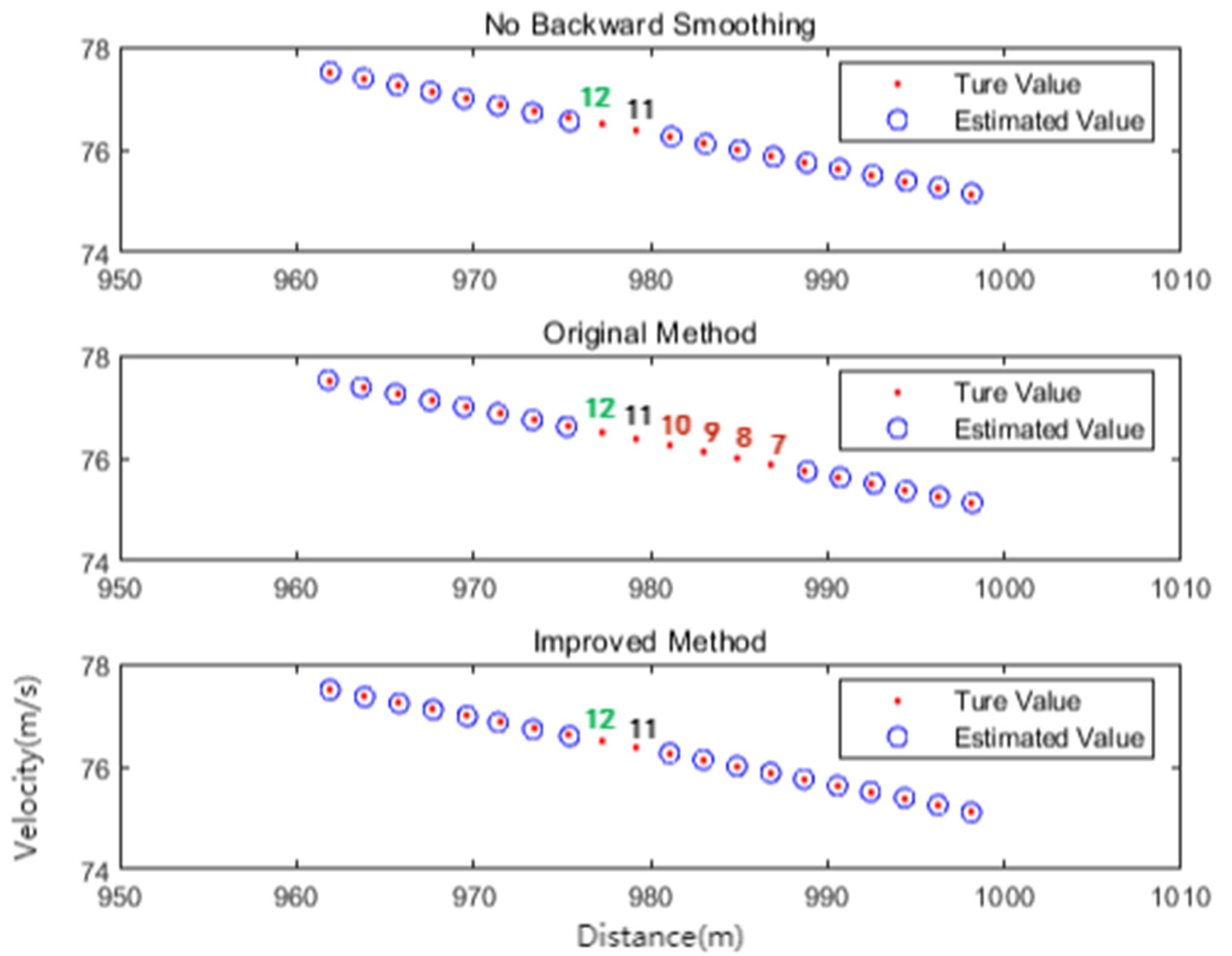
As mentioned above, in order to effectively eliminate the filtered outliers and output the smooth estimated track, the authors of [18] introduced a backward smoothing method combined with label iterative processing (hereafter referred to as the original backward smoothing method). However, this method led to the wrong removal of target estimated points due to missing detection of the target and with the growth of the backward smoothing step, a certain length of track fracture would be formed, thus deteriorating the target tracking performance. In order to intuitively explain the problem of the original backward smoothing method, this paper first conducted a single target simulation experiment according to the parameters set in

Table 2. Scene settings.

Target	Starting Position (m; m/s; m/s2)	Acceleration Description (m/s)
Target 1	[1000; 75; 0]	a (1:20) = 5
Motion noise	0 × [0.5 × T2;T;1]	Measurement noise(m; m/s)	0 × [1.875;0.24]
Clutter quantity	0	Track pruning threshold	0.001
Detection probability	0.95	Backward smoothing step	4
Missing detection description	Z1 (11) missing	Simulation length	20

, which avoided the influences of motion noise, measurement noise, and clutter interference factors (the following simulation experiments further verified that the problems in the original backward smoothing method were not affected by the above factors).

The experiment compared the real and estimated values of the state of the target using the three processing methods: no backward smoothing (N-BS), original backward smoothing (O-BS), and improved backward smoothing (I-BS), as shown in Figure 2. The experiment assumed that the 11th measurement point was missing. It can be seen from the figure that none of the three method had estimated values at the 11th point. In addition, there were no estimated values at the 12th point because the experiment used the measurement-driven target birth method, which was not the focus of discussion here. In addition to the normal number of points 11 and 12, the experimental results of the original backward smoothing method also lacked the estimated values for points 7–10, and the missing length was the same as the backward smoothing step. This was because the original backward smoothing method only retained the target estimation point corresponding to the persistent label to eliminate outliers. When the target was undetected, the corresponding label was also undetected. As a result, undetected targets within the backward smoothing step length were eliminated as outliers, resulting in track breakage, which was the problem in the original backward smoothing method. The improved backward smoothing method perfectly solved this problem.

4.2. Performance Verification

4.2.1. The Influence of the Backward Smoothing Step

On the basis of the simulation experiments in Section 4.1, we further explored the impact of the backward smoothing step size on the target tracking performance of the two backward smoothing methods. The experiment was carried out in the form of Monte Carlo simulation, the simulation times were set to 100, and the final experimental results were analyzed. In this experiment, the influences of motion noise, measurement noise, and clutter interference factors were considered. The specific parameter settings are shown in

Table 3. Scene settings.

Target	Starting Position (m; m/s; m/s2)	Acceleration Description (m/s)
Target 1	[1000; 75; 0]	a (1:20) = 5; a (21:40) = 3; a (41:50) = 1;
Motion noise	1 × [0.5 × T2;T;1]	Measurement noise(m; m/s)	1 × [1.875;0.24]
Clutter quantity	10	Track pruning threshold	0.001
Detection probability	0.9	Backward smoothing step	1,2,3,4,5
Missing detection description	Z1 (25:29) missing	Simulation length	50

. The backward smoothing steps $S_{bs}$ of the experimental variables were 1, 2, 3, 4, and 5, respectively.

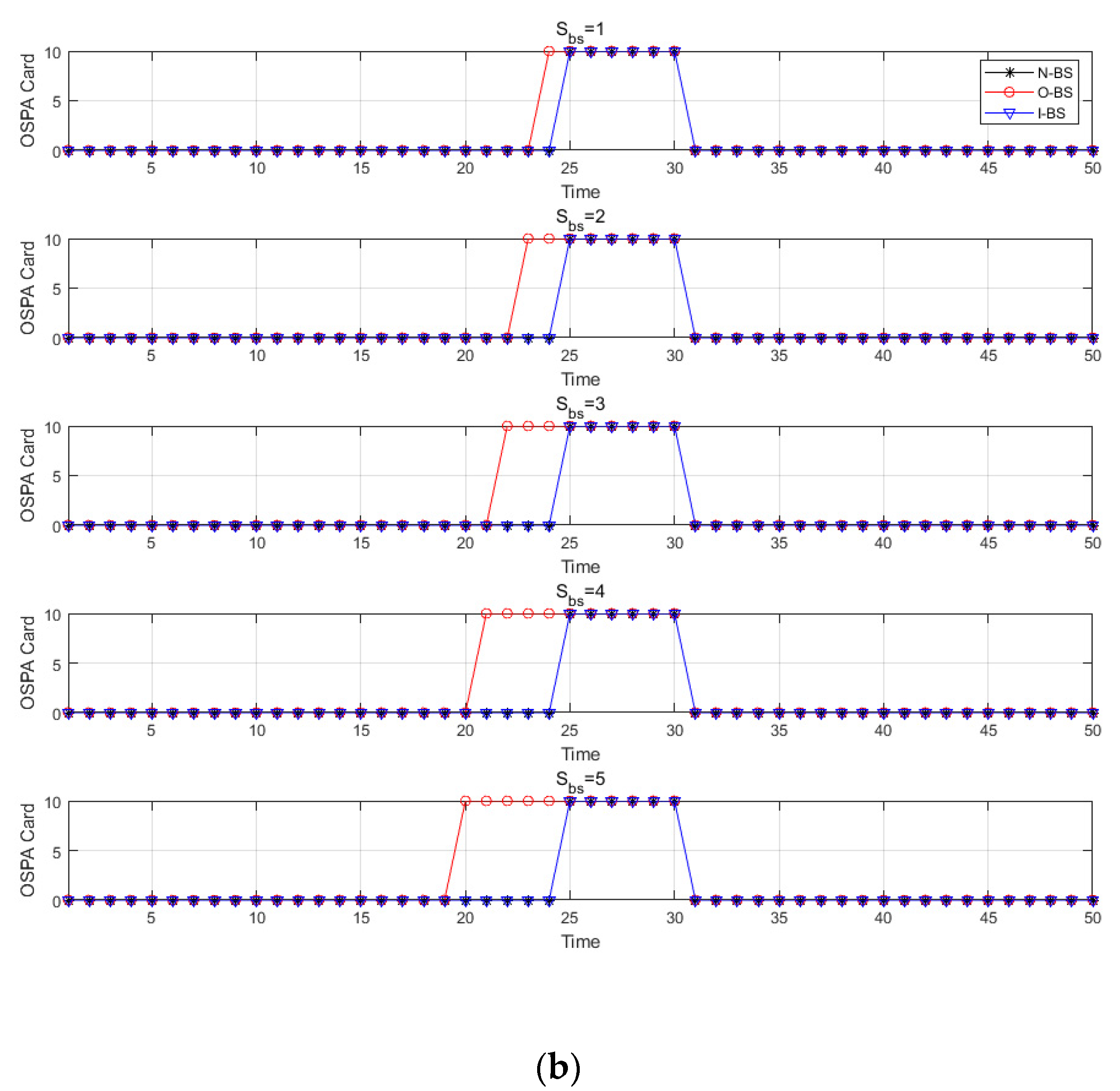
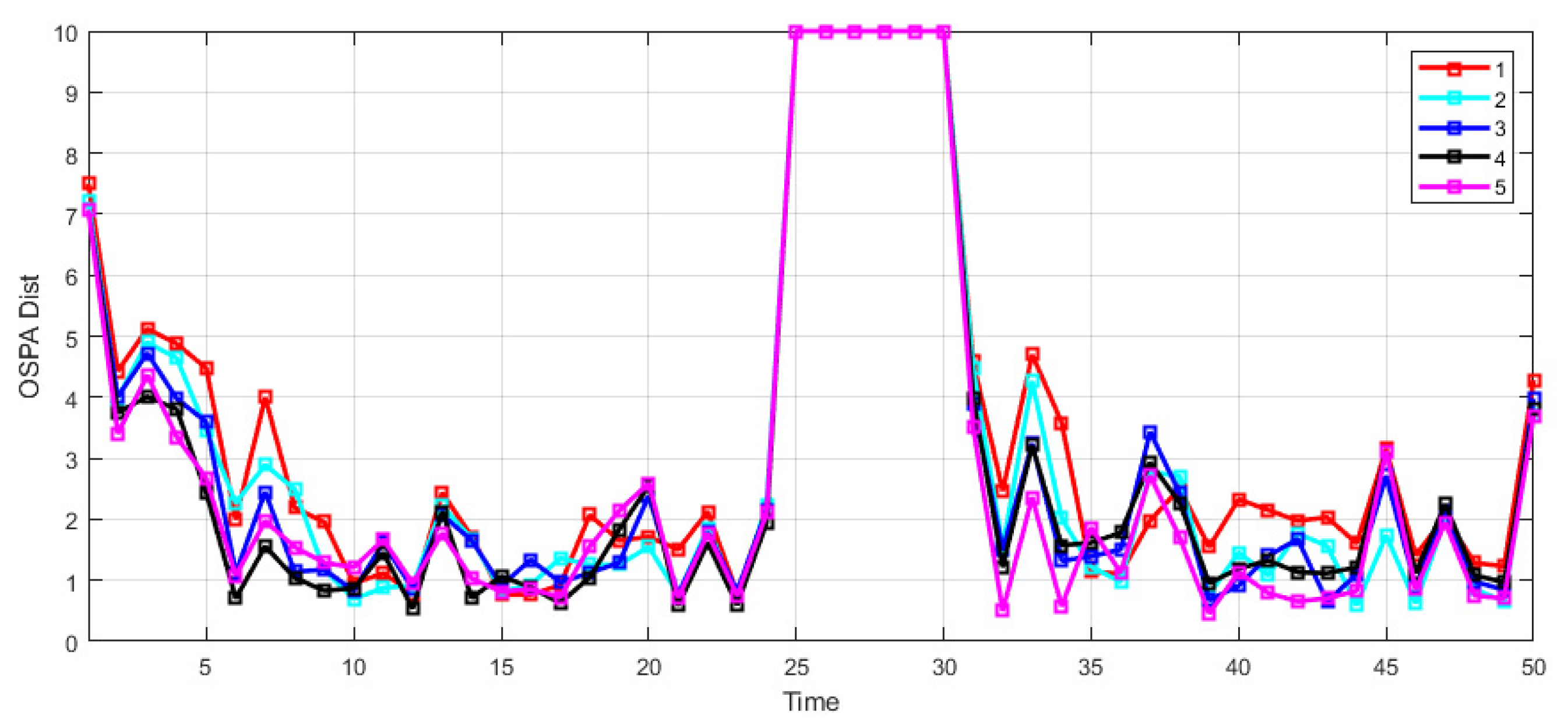
It can be seen from Figure 3b that there were outliers in the estimation results of the non-backward smoothing method, while the other two methods did not have outliers, which verified the ability of the backward smoothing method to eliminate outliers. It was also further verified in Figure 3b and Figure 4 that the original backward smoothing method had the problem of track fracture caused by incorrect elimination of estimated points due to missing detection of the target, and the track fracture was equal to the backward smoothing step. It can be seen from Figure 3a that the tracking performance of the improved backward smoothing method was significantly better than that of the non-backward smoothing method, and it had a certain performance improvement compared with the original backward smoothing method. Figure 5 and Figure 6 show the comparisons of tracking performance and runtime of the proposed methods under different backward smoothing steps. From the experimental results, it could be seen that with the increase in backward smoothing step size, the tracking performance gradually improved, but the increase amplitude gradually decreased and the runtime increased in proportion. Therefore, the setting of the backward smoothing step size should be compromised during processing.

4.2.2. The Influence of the Track Initiation Determination Length

The original backward smoothing processing method wrongly eliminated target points with backward smoothing length due to missing detection, while the improved backward smoothing processing method used this loophole to combine it with track initiation determination to achieve effective processing of invalid short-lived target tracks. In order to illustrate the processing effect, this paper simulated the algorithms of different track start decision lengths. The parameter settings are shown in

Table 4. Scene settings.

Target	Starting Position (m; m/s; m/s2)	Acceleration Description (m/s)
Target 1	[1000; 75; 0]	a (1:20) = 5; a (21:40) = 3; a (41:50) = 1;
Jamming target 1	[1020; 78; 0]	a (8:10) = 5; (3 points)
Jamming target 2	[990; 77; 0]	a (17:20) = 5; (4 points)
Jamming target 3	[920; 76; 0]	a (27:31) = 5; (5 points)
Jamming target 4	[930; 80; 0]	a (38:43) = 5; (6 points)
Motion noise	0 × [0.5 × T2;T;1]	Measurement noise(m; m/s)	0 × [1.875;0.24]
Clutter quantity	10	Track pruning threshold	0.001
Detection probability	0.9	Backward smoothing step	6
Missing detection description	Z1 (25:29) missing	Simulation length	50

, and the track start decision lengths $L_{tid}$ were taken as 3, 4, 5, and 6, respectively. The simulation results are shown in Figure 7. In order to intuitively show the problem, the experiment also avoided the influences of motion noise, measurement noise, and clutter (the following simulation experiments further verified that the problems in the original backward smoothing method were not affected by the above factors).

In the experiment, in addition to normal target 1, there were also jamming targets 1–4, which formed short tracks with lengths of 3, 4, 5, and 6, respectively. It can be seen from Figure 7 that with the gradual increase in track initiation determination length setting, the tracks of jamming targets 1–4 with different lengths of 3, 4, 5, and 6 were eliminated one by one, while the normal targets were not affected. The above result verified the role of the improved backward smoothing method in track initiation determination and invalid short-lived track elimination. In addition, the initial determination length of the track only played a role in determining whether the track was effective. The specific elimination function and length depended on the backward smoothing length. Therefore, in the process of setting the algorithm parameters, the initial determination length of the track should not be greater than the backward smoothing length, and the above parameter should be set according to the actual scene.

4.3. Multi-Target Scene Simulation

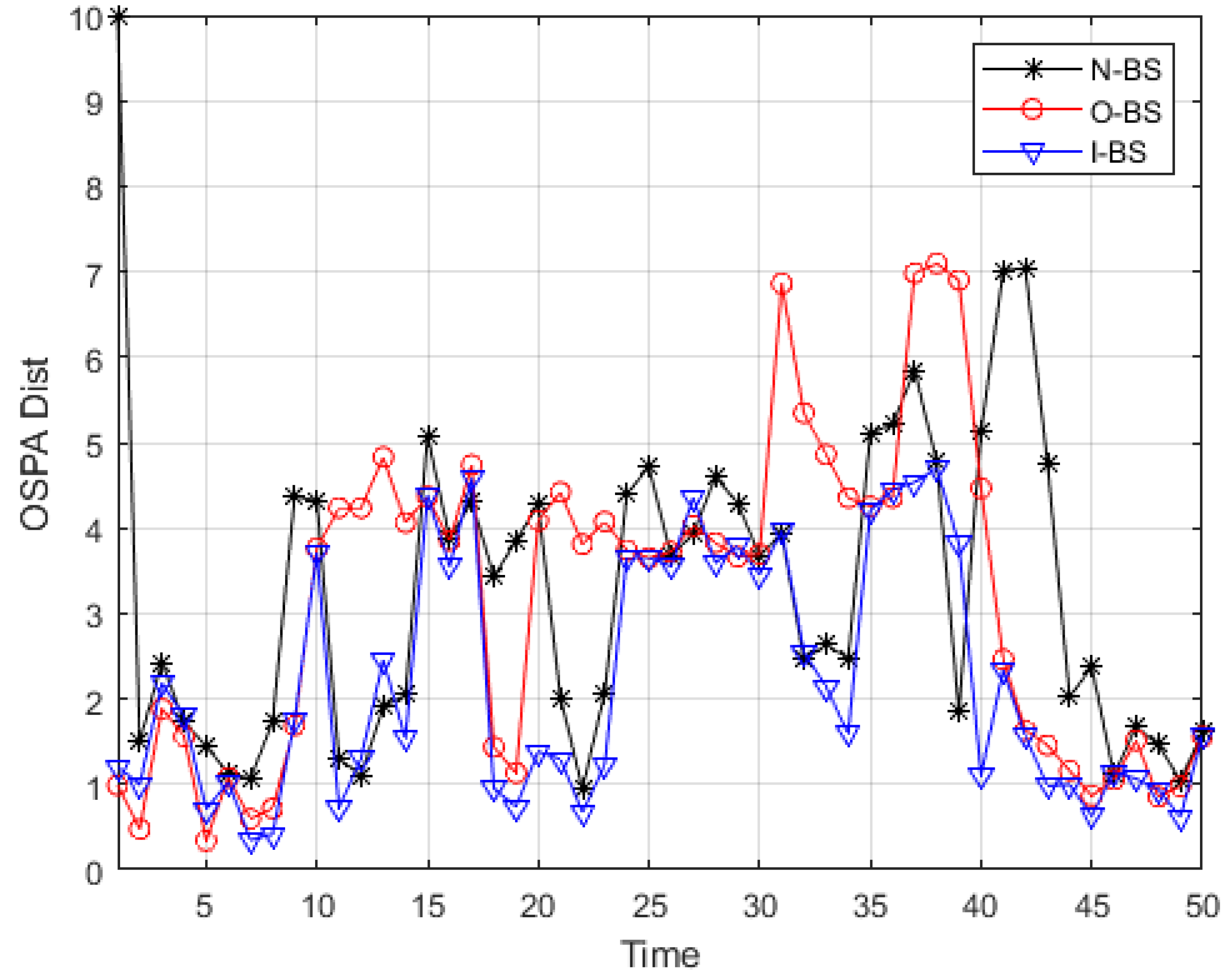
In order to further verify the multi-target tracking performance of the improved method, a multi-target simulation experiment with the parameters set in

Table 5. Scene settings.

Target	Starting Position (m; m/s; m/s2)	Acceleration Description (m/s)
Target 1	[1000; 75; 0]	a (1:20) = 5; a (21:40) = 3; a (41:50) = 1;
Target 2	[1020; 70; 0]	a (1:25) = 5; a (26:50) = 3;
Target 3	[980; 68; 0]	a (1:30) = 3; a (31:50) = 1;
Jamming target 1	[1000; 70; 0]	a (8:10) = 5; (3 points)
Jamming target 2	[990; 77; 0]	a (17:20) = 3; (4 points)
Jamming target 3	[920; 76; 0]	a (27:31) = 1; (5 points)
Jamming target 4	[930; 80; 0]	a (38:43) = 1; (6 points)
Jamming target 5	[940; 72; 0]	a (38:42) = −3; (6 points)
Jamming target 6	[920; 69; 0]	a (38:42) = −5; (6 points)
Motion noise	1 × [0.5 × T2;T;1]	Measurement noise(m; m/s)	1 × [1.875;0.24]
Clutter quantity	5	Track pruning threshold	0.001
Detection probability	0.76	Backward smoothing step	6
Missing detection description	Z1 (35:38,1) missing Z3 (15:16;24:30,2) missing	Simulation length	50

was carried out. The experiment included three targets, six short-lived jamming targets, and clutter. The experiment still carried out Monte Carlo simulation experiments with 100 simulation times, and the final experimental results were analyzed. The experimental results are shown in Figure 8, Figure 9 and Figure 10.

Table 6. The total OSPA errors of three methods.

Method	OSPA Dist Error	OSPA Card Error	OSPA Loc Error
N-BS smoother	134.1907	53.2	80.9907
O-BS smoother	141.939	90.6667	51.2724
I-BS smoother	102.4238	45.3333	57.0905

shows the total OSPA error of all methods over the entire time period for all of the Monte Carlo simulation experiments, for which the OSPA distance error was equal to the OSPA location error plus the OSPA cardinality error.

From the experimental results, it could be seen that the improved backward smoothing method could accurately estimate the number of targets, which was mainly due to its function of removing outliers and invalid short-lived tracks. In addition, it could be seen from Figure 10 and Table 6 that the tracking performance of the improved backward smoothing method was better than that of the other two methods.

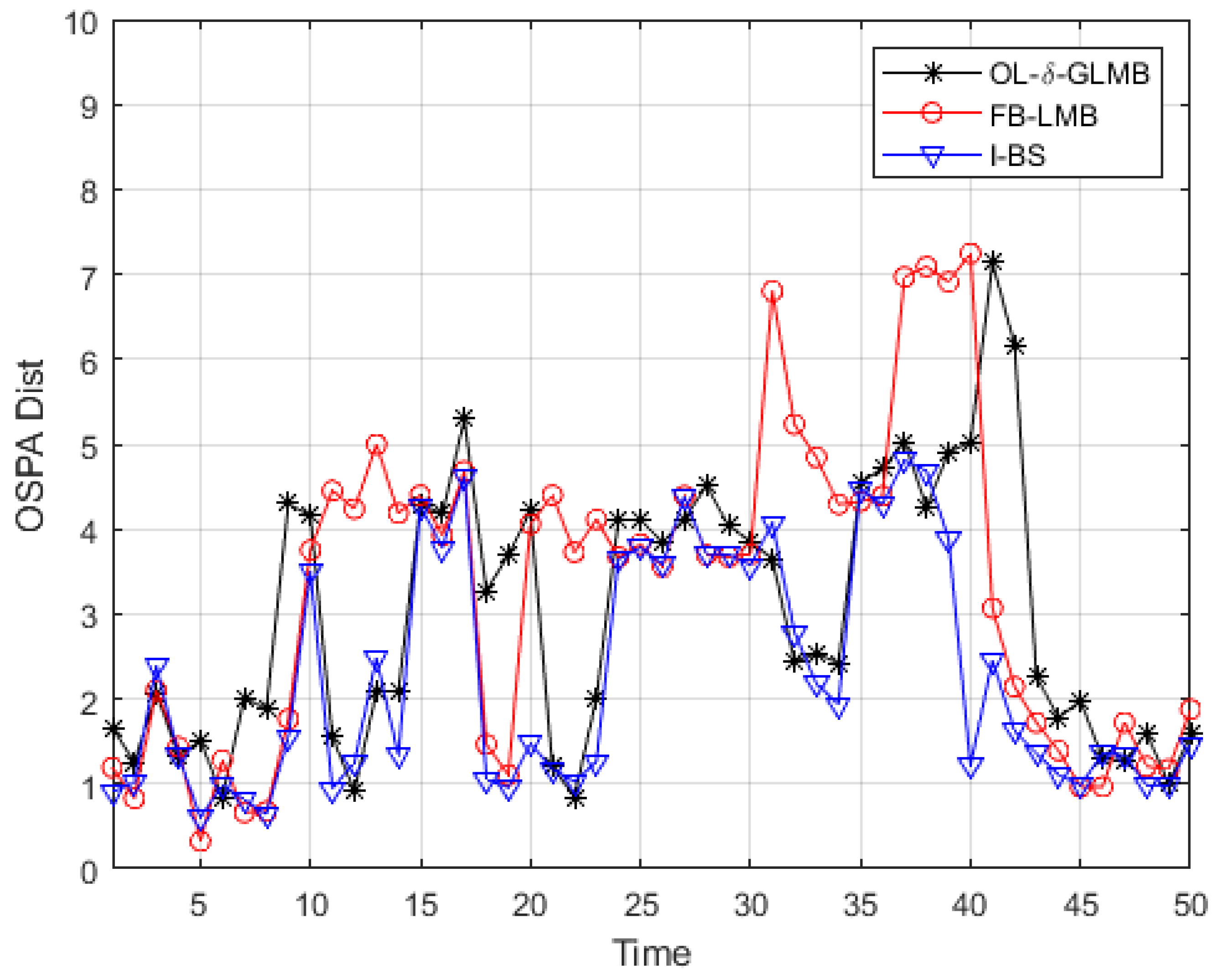
On this basis, this paper compared the proposed method with the OL-δ- GLMB smoother (One Time Step Lagged δ-GLMB Smoother [14]) and the FB-LMB smoother (Forward Backward LMB [17]). The authors of [14] provided a detailed comparison of the proposed OL-δ-GLMB smoother, LMB smoother [16], δ-GLMB-A smoother [27] smoother, and δ-GLMB filter [28] and verified its great performance. The authors of [17] thoroughly compared the tracking performance of the proposed FB-LMB smoother with that of the LMB filter, PHD filter, PHD smoother, CB-MeMBer filter, and MB smoother, verifying its effectiveness. This paper aimed to further validate the effectiveness of the proposed algorithm by comparing it with the two methods mentioned above.

In Figure 11 and Figure 12, the OSPA distance and cardinality estimation results of three methods are presented. Combined with the total OSPA distance error, total OSPA cardinality error, and total OSPA location error of each method shown in

Table 7. The total OSPA errors of three methods.

Method	OSPA Dist Error	OSPA Card Error	OSPA Loc Error	Runtime(s)
OL-δ-GLMB smoother	150.824	66.5	84.324	6.385
FB-LMB smoother	164.6057	113.333	51.2724	18.52
I-BS smoother	113.7572	56.667	57.0905	23.4

, it could be seen that the proposed algorithm had better cardinality estimation performance than the other two methods due to correctly eliminating the outliers and invalid short-lived tracks, which could be seen from the total OSPA cardinality error. Due to the improvement in cardinality estimation performance, the total OSPA distance was also better than that obtained by the other two smoothers, indicating that the proposed method had better tracking performance.

4.4. Verification of Measured Data

The measured data used in this paper were from the same source as the data used in [18], thus enabling comparative experiments to be carried out in order to verify the improvement of the proposed algorithm. Table 1 lists the radar parameters. The basic parameter settings of the measured data scene are shown in

Table 8. Scene settings.

Target	Starting Position (m; m/s; m/s2)	Simulation Length	40
Target 1	[1290; 40.43; 0]	Backward smoothing step	5
Target 2	[1148; 84.24; −4]	Clutter quantity	4
Clutter quantity	0.5 × [0.5 × T2;T;1]	Measurement noise(m; m/s)	1 × [1.875;0.24]
Detection probability	0.9	Track pruning threshold	0.001, 0.1, 0.3, 0.5

. Monte Carlo simulation experiments were conducted for 100 times, and the final experimental results were analyzed. The simulation results are shown in Figure 13, Figure 14, Figure 15 and Figure 16.

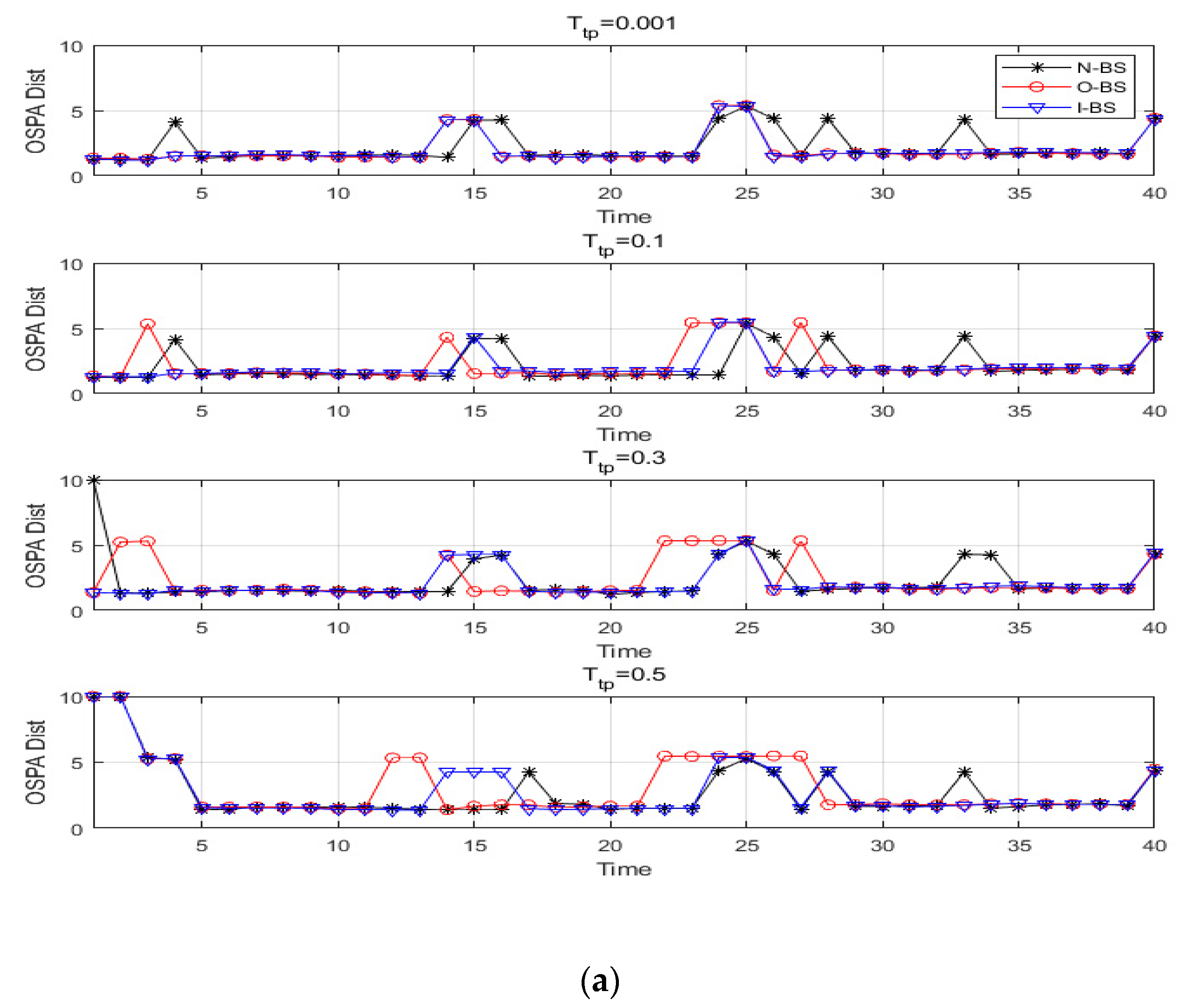
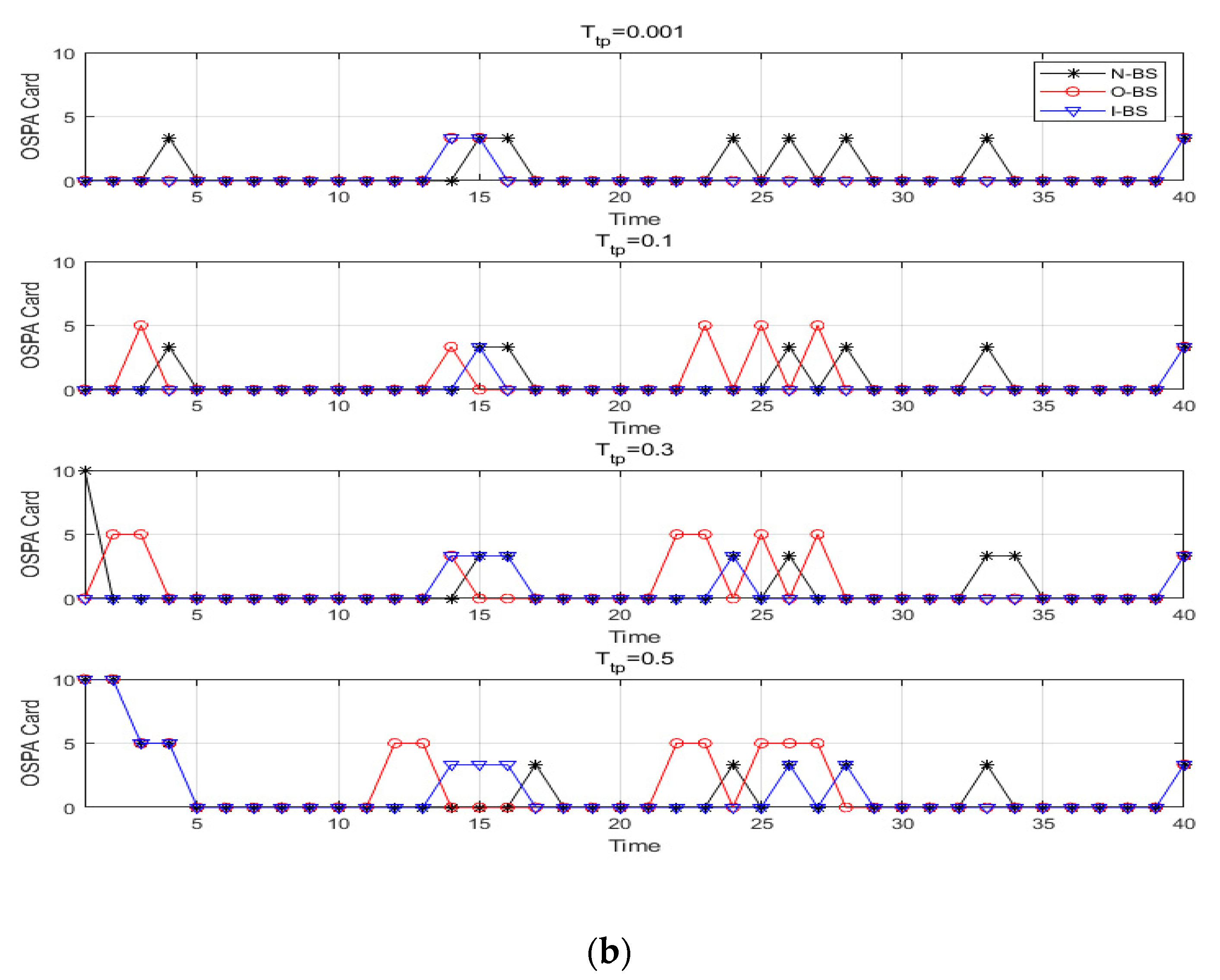
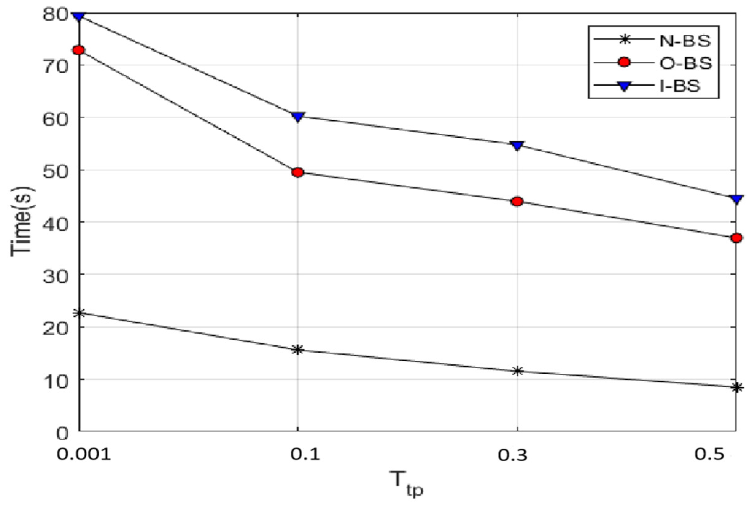
The measured data included two targets, for which the real and measured values of the target states are shown in Figure 13. There was a velocity ambiguity in the measured data. In this paper, the corresponding estimation points were selected directly according to the prior information, regardless of the specific velocity ambiguity resolution process. In addition to the average OSPA distance and cardinality estimation results with a track pruning threshold $T_{tp}$ of 0.001, the verification experiments of the measured data also gave experimental results for 0.1, 0.3, and 0.5. This was because the original backward smoothing process chose a lower track pruning threshold to reduce the impact of missed detection of the target in order to reduce the impact of missing detection, but this caused the algorithm to retain too many track assumptions in the process, which reduce the operation efficiency of the algorithm. The improved backward smoothing method solved the problems in the original backward smoothing method, so that the threshold value of track pruning need not be reduced too much, thus ensuring the processing efficiency of the algorithm. It can be seen from Figure 14 and Figure 16 that when the track pruning threshold was 0.001, the original method was similar to the improved method in terms of algorithm performance. However, when the track pruning threshold was 0.1, the performance of the original method began to deteriorate whereas the improved method still maintained good tracking performance. When the track pruning threshold was 0.3 or 0.5, the tracking performance of all methods dropped rapidly, and the original method deteriorated more seriously. This was caused by its own problems. The high track pruning threshold resulted in the loss of a large number of target estimation points, which seriously affected the tracking performance. From the point of view of processing time, reducing the track pruning threshold could reduce the processing time, but a low track pruning threshold would deteriorate the tracking performance. From the further analysis of the above experimental results, it could be concluded that the tracking performance of the improved method with a track pruning threshold of 0.1 was close to that of the original method with a track pruning threshold of 0.001, but the runtime was obviously shorter, which reflected the improved performance in processing efficiency.

Based on the above analysis results and experimental data, this paper further compared the proposed method with the OL-δ-GLMB smoother and FB-LMB smoother. The experimental results are shown Figure 17 and

Table 9. The total OSPA errors and runtimes of three methods.

Method	OSPA Dist Error	OSPA Card Error	OSPA Loc Error	Runtime(s)
OL-δ-GLMB smoother	87.9549	33.3333	54.6216	30.47
FB-LMB smoother	90.4184	28.3333	62.0851	78.75
I-BS smoother	82.1882	13.3333	68.8549	67.53

.

From the experimental results, it could be seen that the proposed algorithm had better cardinality estimation performance than the other two methods, which was consistent with the results of the multi-target simulation experiments in Section 4.3. This was entirely due to the effective handling of outliers and tracks, making the proposed method superior to the OL-δ-GLMB smoother and FB-LMB smoother in overall tracking performance.

5. Conclusions

In order to optimize the impact of false alarm/outlier and track initiation on radar multi-target tracking performance, this paper proposed an improved backward smoothing method based on label iterative processing on the basis of the LMB filter. This method corrected the problems in the original backward smoothing method in [18], effectively eliminated the filtered outliers, and outputted a smoothing estimated track. The method also incorporated the function of track initiation determination, which could sequentially process short-lived tracks and reduce the computational burden of real-time processing. The numerical analysis results showed that the proposed method could correctly remove outliers and invalid short-lived tracks, improve the accuracy of target cardinality and state estimations to a certain extent, and further improve the processing efficiency of the algorithm by reducing the track pruning threshold. During the research process, it was found that using label iterative processing could help the labeled-RFS-class filter/smoother achieve sequential processing of tracks, which is of great significance for batch processing, thus solving the problems of track initiation determination and track continuity processing in conventional methods without track output. Therefore, we plan to further explore the use of label iterative processing to achieve target track continuity processing. At the theoretical level, mature fast-processing methods were introduced to reduce the computational burden of the labeled-RFS theory based filter/smoother and promote its application in practical engineering.

References

1. Cai, F. Research on Detection and Tracking Technologies for Dim-Targets in Radar. Ph.D. Thesis, National University of Defense Technology, Changsha, China, 2015. (In Chinese). [Google Scholar]
2. Mahler, R.P.S.; Ebrary, I. Statistical Multisource-Multitarget Information Fusion; Artech House Publishers: Boston, MA, USA, 2007. [Google Scholar]
3. Mahler, R.P.S. Multi-target Bayes Filtering via First-Order Multi-target Moments. IEEE Trans. Aerosp. Electron. Syst. 2003, 39, 1152–1178. [Google Scholar] [CrossRef]
4. Mahler, R.P.S. Filters of Higher Order in Target Number. IEEE Trans. Aerosp. Electron. Syst. 2007, 43, 1523–1543. [Google Scholar] [CrossRef]
5. Vo, B.T.; Vo, B.N.; Cantoni, A. The Cardinality Balanced Multi-Tar-get Multi-Bernoulli Filter and Its Implementations. IEEE Trans. Signal Process. 2009, 57, 409–423. [Google Scholar]
6. Vo, B.T.; Vo, B.N. Labeled Random Finite Sets and Multi-Object Conjugate Priors. IEEE Trans. Signal Process. 2013, 61, 3460–3475. [Google Scholar] [CrossRef]
7. Reuter, S.; Vo, B.N.; Dietmayer, K. The Labeled Multi-Bernoulli Filter. IEEE Trans. Signal Process. 2014, 62, 3246–3260. [Google Scholar]
8. Vo, B.T.; Clark, D.; Vo, B.N.; Ristic, B. Bernoulli Forward-Backward Smoothing for Joint Target Detection and Tracking. IEEE Trans. Signal Process. 2011, 59, 4473–4477. [Google Scholar] [CrossRef]
9. Vo, B.N.; Vo, B.T.; Mahler, R.P.S. Closed-Form Solutions to Forward–Backward Smoothing. IEEE Trans. Signal Process. 2011, 60, 2–17. [Google Scholar] [CrossRef]
10. Nagappa, S.; Delande, E.D.; Clark, D.E.; Houssineau, J. A Tractable Forward-Backward CPHD Smoother. IEEE Trans. Aerosp. Electron. Syst. 2017, 53, 201–217. [Google Scholar] [CrossRef]
11. Dong, L.; Hou, C.; Yi, D. Multi-Bernoulli Smoother for Multi-target Tracking. Aerosp. Sci. Technol. 2016, 48, 234–245. [Google Scholar]
12. Beard, M.; Vo, B.T.; Vo, B. Generalised Labelled Multi-Bernoulli Forward-Backward Smoothing. In Proceedings of the 2016 19th International Conference on Information Fusion (FUSION), Heidelberg, Germany, 5–8 July 2016; pp. 688–694. [Google Scholar]
13. Vo, B.-N.; Vo, B.-T. A Multi-Scan Labeled Random Finite Set Model for Multi-Object State Estimation. IEEE Trans. Signal Process. 2019, 67, 4948–4963. [Google Scholar] [CrossRef]
14. Liang, G.; Li, Q.; Qi, B.; Qiu, L. Multi-target Tracking Using One Time Step Lagged Delta-Generalized Labeled Multi-Bernoulli Smoothing. IEEE Access 2020, 8, 28242–28256. [Google Scholar] [CrossRef]
15. Liu, R.; Fan, H.Q.; Li, T.C.; Xiao, H. A Computationally Efficient Labeled Multi-Bernoulli Smoother for Multi-Target Tracking. Sensors 2019, 19, 4226. [Google Scholar] [CrossRef] [PubMed]
16. Liu, R.; Fan, H.Q.; Xiao, H.T. A Forward-Backward Labeled Multi-Bernoulli Smoother. In Proceedings of the 16th International Conference on Distributed Computing and Artificial Intelligence, Avila, Spain, 26–28 June 2019; pp. 244–252. [Google Scholar]
17. Liu, R. Research on Radar Target Tracking with Labeled Random Finite Sets. Ph.D. Thesis, National University of Defense Technology, Changsha, China, 2020. (In Chinese). [Google Scholar]
18. Liang, P.; Liu, R.; Chen, X.; Shang, Z.; Yi, T.; Lu, D. Radar Weak Target Tracking Based on LMB Smoothing. Aero Weapon. 2021, 28, 80–85. [Google Scholar]
19. Li, X. A Study of Radar Target Detection under Heterogeneous Background. Master’s Thesis, Xi’an University of Electronic Science and Technology, Xi’an, China, 2020. [Google Scholar]
20. Rahamathullah, A.S.; Garcia-Fernandez, A.F.; Svensson, L. Generalized optimal sub-pattern assignment metric. In Proceedings of the 2017 20th International Conference on Information Fusion (Fusion), Xi’an, China, 10–13 July 2017; pp. 1–8. [Google Scholar]
21. Anil, K.J. Data clustering: 50 years beyond K-means. Pattern Recognit. Lett. 2010, 31, 651–666. [Google Scholar]
22. Vo, B.N.; Ma, W.K. The Gaussian mixture probability hypothesis density filter. IEEE Trans. Signal Process. 2006, 54, 4091–4104. [Google Scholar] [CrossRef]
23. Doucet, A.; Freitas, N.; Gordon, N. Sequential Monte Carlo Methods in Practice; Springer: Berlin/Heidelberg, Germany, 2001. [Google Scholar]
24. Arulampalam, M.S.; Maskell, S.; Gordon, N.; Clapp, T. A tutorial on particle filters for online nonlinear/non-Gaussian Bayesian tracking. IEEE Trans. Signal Process. 2002, 50, 174–188. [Google Scholar] [CrossRef]
25. Gning, A.; Ristic, B.; Mihaylova, L.; Abdallah, F. An introduction to box particle filtering. IEEE Signal Process. Mag. 2013, 30, 165–170. [Google Scholar] [CrossRef]
26. Schuhmacher, D.; Vo, B.-T.; Vo, B.-N. A consistent metric for performance evaluation of multi-object filters. IEEE Trans. Signal Process. 2008, 56, 3447–3457. [Google Scholar] [CrossRef]
27. Li, Q.-R.; Qi, B.; Liang, G.-L. Approximate Bayes multi-target tracking smoother. IET Radar Sonar Navigat. 2019, 13, 428–437. [Google Scholar] [CrossRef]
28. Vo, B.-N.; Vo, B.-T.; Phung, D. Labeled random finite sets and the Bayes multi-target tracking filter. IEEE Trans. Signal Process. 2014, 62, 6554–6567. [Google Scholar] [CrossRef]
Figure 1. Processing flow chart of improved backward smoothing method based on LMB filtering.
Remotesensing 15 02438 g001
Figure 2. Effect description of the proposed method.
Remotesensing 15 02438 g002
Figure 3. (a) Real and measured values of target states. (b) State estimation result of three methods with different backward smoothing steps (the results of the non-backward smoothing method are introduced on the left for comparison).
Remotesensing 15 02438 g003aRemotesensing 15 02438 g003b
Figure 4. (a) Average OSPA distances under different backward smoothing steps of three methods. (b) Average OSPA cardinality estimations under different backward smoothing steps of three methods.
Remotesensing 15 02438 g004aRemotesensing 15 02438 g004b
Figure 5. Average OSPA distances of the improved method under different backward smoothing steps.
Remotesensing 15 02438 g005
Figure 6. Comparison of runtimes of three methods.
Remotesensing 15 02438 g006
Figure 7. Processing results of different track initial determination lengths.
Remotesensing 15 02438 g007
Figure 8. (a) Real and measured values of target states. (b) Processing results of three methods.
Remotesensing 15 02438 g008
Figure 9. Cardinality estimations of three processing methods.
Remotesensing 15 02438 g009
Figure 10. OSPA distances of three methods.
Remotesensing 15 02438 g010
Figure 11. OSPA distances of three methods.
Remotesensing 15 02438 g011
Figure 12. Cardinality estimations of three methods.
Remotesensing 15 02438 g012
Figure 13. Comparison of real and measured values of measured-data target states.
Remotesensing 15 02438 g013
Figure 14. (a) OSPA distances of three methods under different track pruning thresholds. (b) OSPA cardinality estimations of three methods under different track pruning thresholds.
Remotesensing 15 02438 g014aRemotesensing 15 02438 g014b
Figure 15. Runtimes of three methods under different track pruning thresholds.
Remotesensing 15 02438 g015
Figure 16. The total OSPA errors of three methods under different track pruning thresholds.
Remotesensing 15 02438 g016
Figure 17. (a) OSPA distances of three methods. (b) OSPA cardinality estimations of three methods.
Remotesensing 15 02438 g017