Sentinel-2 and Sentinel-1 Bare Soil Temporal Mosaics of 6-Year Periods for Soil Organic Carbon Content Mapping in Central France

Abstract

Satellite-based soil organic carbon content (SOC) mapping over wide regions is generally hampered by the low soil sampling density and the diversity of soil sampling periods. Some unfavorable topsoil conditions, such as high moisture, rugosity, the presence of crop residues, the limited amplitude of SOC values and the limited area of bare soil when a single image is used, are also among the influencing factors. To generate a reliable SOC map, this study addresses the use of Sentinel-2 (S2) temporal mosaics of bare soil (S2Bsoil) over 6 years jointly with soil moisture products (SMPs) derived from Sentinel 1 and 2 images, SOC measurement data and other environmental covariates derived from digital elevation models, lithology maps and airborne gamma-ray data. In this study, we explore (i) the dates and periods that are preferable to construct temporal mosaics of bare soils while accounting for soil moisture and soil management; (ii) which set of covariates is more relevant to explain the SOC variability. From four sets of covariates, the best contributing set was selected, and the median SOC content along with uncertainty at 90% prediction intervals were mapped at a 25-m resolution from quantile regression forest models. The accuracy of predictions was assessed by 10-fold cross-validation, repeated five times. The models using all the covariates had the best model performance. Airborne gamma-ray thorium, slope and S2 bands (e.g., bands 6, 7, 8, 8a) and indices (e.g., calcareous sedimentary rocks, “calcl”) from the “late winter–spring” time series were the most important covariates in this model. Our results also indicated the important role of neighboring topographic distances and oblique geographic coordinates between remote sensing data and parent material. These data contributed not only to optimizing SOC mapping performance but also provided information related to long-range gradients of SOC spatial variability, which makes sense from a pedological point of view.

1. Introduction

Cropland soils cover a total of ~1500 million hectares worldwide, distributed across different agroecosystems and climatic conditions, as well as diverse cropping systems and management practices [1]. Soil organic carbon (SOC) monitoring in croplands is crucial for climate change mitigation and food security [2,3]. The four per 1000 global initiative has increased interest in more sustainable soil management and conservation in agricultural regions [4]. For about 20 years, the high demand for detailed soil information for policy implementation has driven digital soil mapping (DSM, [5]). For instance, projects such as SoilGrids [6,7] and GlobalSoilMap [8,9,10] aim, through different approaches and techniques, to produce soil property maps over the entire globe. Chen et al. [11] recently published a review of GlobalSoilMap products on a broad scale, and SOC was the target soil property with the highest number of studies.

The use of satellite imagery to estimate SOC has been widely used, including bands from the Satellite Pour l’Observation de la Terre (SPOT) [12], the Thematic Mapper (TM) imaging system of the Landsat satellite [13], and more recently, studies of spectra obtained from bare soil imagery by Sentinel-2 (S2) [14,15,16]. The S2 mission of the EU Copernicus program is a constellation of two satellites (Sentinel-2A and Sentinel-2B) launched in 2015 and 2017, respectively. Both satellites are equipped with the Multi-Spectral Instrument (MSI), with a revisit period of every 5 days and spatial resolutions of 10 m (bands 2, 3, 4 and 8) and 20 m (bands 5, 6, 7, 8A, 11 and 12). These high resolutions open up a wide range of applications, such as SOC mapping in crop soils. Some previous studies at local and regional scales using S2 images in Brazil [17], Belgium [18], France [16,19,20], the Czech Republic [15,21] and Germany [14] reported that the capability of S2 images to predict SOC performed better in some regions with different environmental and pedological characteristics than in others. For example, Vaudour et al. [20] reported different performances in two different regions in France: Versailles Plain (R² of 0.56, RMSE of 1.23 g.kg⁻¹) and La Peyne Valley (R² of 0.02, RMSE of 3.71 g.kg⁻¹).

SOC mapping is generally hampered by several reasons: (i) low sample density for model calibration due to time and high analysis costs; (ii) soil sampling period of legacy data, when intensive agriculture and soil management practices vary over a period [19]; (iii) impact of topsoil conditions and acquisition date of satellite imagery [16,19]; (iv) area of bare soil limited or covered by crop vegetation from single date images [16,22]; and (v) heterogeneous sampling in space and the presence of sampling clusters. Alternatives to overcome some of these issues have been proposed, for example, choosing the best period of the cropping calendar to use images between sowing and emergence [18] or extending the bare soil area through composite imaging using spectral indices alone [22,23,24,25] or in combination with values of soil moisture products (SMPs) derived from Sentinel 1 and 2 images [22]. However, there is still a gap related to the study of the ability to detect SOC via satellite images over large regional areas influenced by different soil-landscape formations, altitude, parent material, land-use history and management practices, which is crucial to supporting national or global mapping projects. Therefore, some frequent questions are, for example, (i) is it feasible or not to use S2 imagery to map SOC in a particular area where there might be a large or narrow spectral variation (e.g., an area X with different landforms or a flat area Y with a large or slight variation of soil classes)? Or (ii) which environmental covariates are relevant and how do they help to map SOC spatial variability? Addressing these questions is important not only to optimize model prediction performances but also to understand in which cases (X or Y area) it is more or less useful to use satellite spectral data to support SOC digital mapping.

The Beauce region, located southwest of Paris, is a limestone plateau known as “the granary of France” for its large production of cereal crops for more than 50 years at least [26]. Cambisols and Luvisols are the main soil classes in this region. In addition, it is common to find silt, silt loam, or silt clay loam layers derived from sediments formed by peri-glacial winds that redistributed loess deposits across the area [27]. A higher SOC content favors aggregate stability, i.e., there is greater physical stability that promotes soil structure, which is important in agriculture (e.g., [28,29]). SOC improves water retention and drainage capacity, soil aeration and reduces the risk of erosion and nutrient loss by leaching [30]. Knowing SOC is essential for agricultural soil management practices such as the application of exogenous organic matter (EOM, e.g., manure and green waste compost) to increase organic carbon and supply crop nutrient demand [31]. Therefore, there is a need to provide accurate information on SOC content variability through remote sensing data to contribute to the elaboration of maps of soil carbon status in agricultural regions, especially since organic amendment spreading is increasingly common in agricultural regions [32].

The overall objective of this study is to assess the capability of Sentinel-2 imagery to map top SOC content over croplands in the Beauce region of France. In order to achieve this, we addressed (i) the use of S2 temporal mosaics of bare soil (S2Bsoil) over a 6-year period; (ii) the use of soil moisture maps (SMPs) estimated at plot scale from Sentinel-1/2 images; and (iii) the use of legacy data and a number of environmental covariates derived from the digital elevation model, remote sensing data, lithology (soil parent material) maps and airborne gamma-ray data. In addition to intending to generate a reliable SOC map at a 25-m resolution, this paper also aims to answer two questions: (i) is it worthwhile to construct temporal mosaics of bare soils considering as many dates as possible or selecting dates using criteria such as soil moisture and periods with different soil management practices instead to obtain a better modeling performance? Additionally, (ii) in such an intensively managed agricultural region, is it possible, through DSM, to determine if the use of legacy data and environmental covariates explains the SOC variability and which set of covariates is more relevant?

2. Materials and Methods

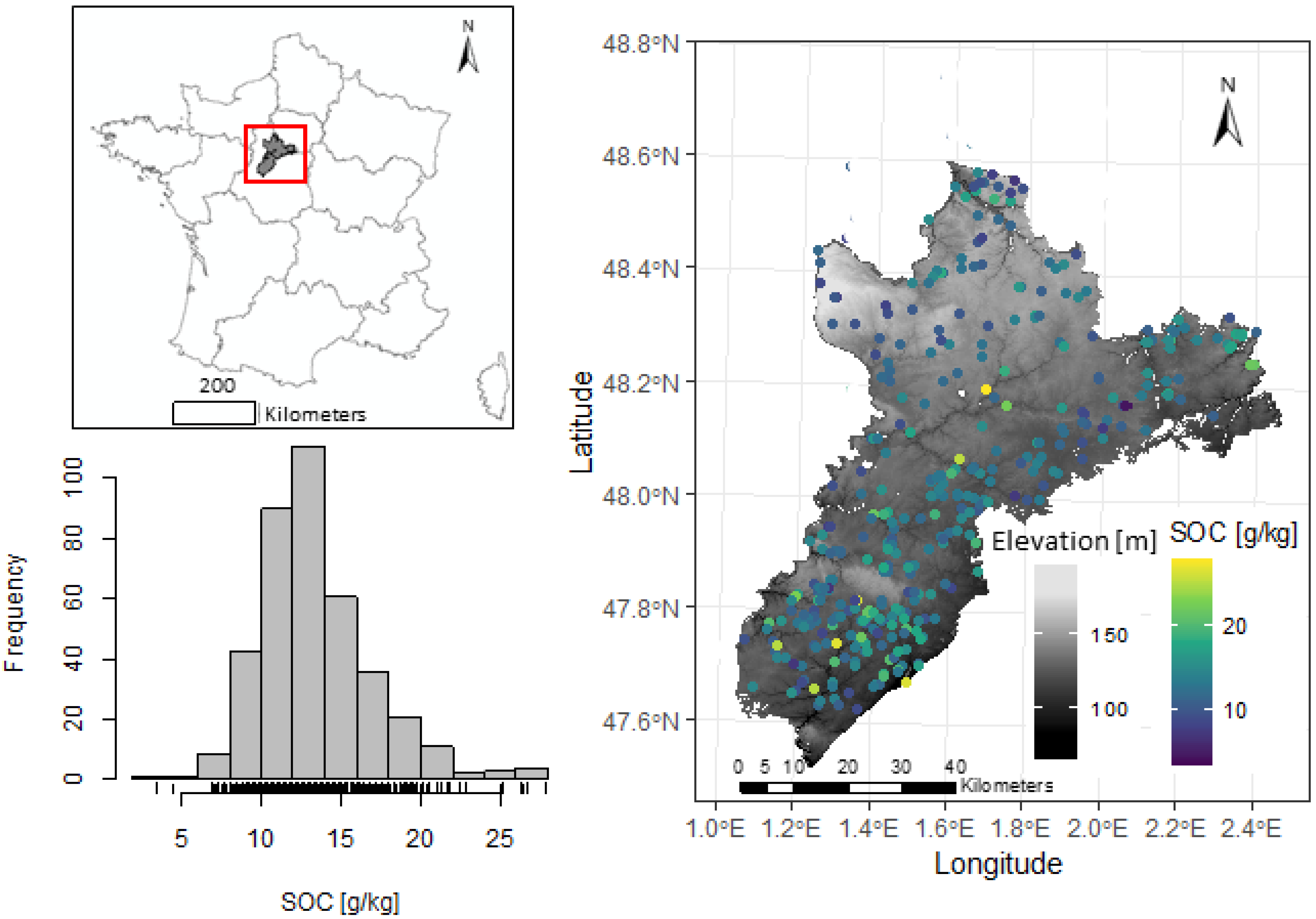
2.1. Study Area and Soil Data

This study was conducted in the administrative region of Centre Val de Loire, southwest of Paris, in an agricultural region known as “Beauce”, covering 4838 km² (Figure 1). The Land Parcel Identification System (LPIS, in French, “registre parcellaire graphique”) of 2019 (French National Institute of Geographic and Forest Information (IGN)) determined that about 84% of the total area consists of croplands. Different crops are cultivated, mainly winter cereals and malting barley, with crop rotations: rapeseed, sugar beet, maize, or vegetables [33]. This study area covers three departments (Eure-et-Loir, Loir-et-Cher and Loiret) and is located over the Beauce aquifer, one of the main groundwater reservoirs in France [34]. The climate is continental–oceanic, with a mean annual temperature of 11.5 °C and a mean annual rainfall of 700 mm [35]. Cambisols and Luvisols are the main soil classes observed in the region [36]. These soils are developed from loess deposits that covered a bedrock of tertiary continental lacustrine limestone that was karstified and slightly weathered [37]. However, some Podzols, Gleysols, Fluvisols, Arenosols and Vertisols are more locally present, mainly at the southern border of the region.

We used the LPIS system to identify and use 391 cropland topsoil samples from two databases used for DSM in France (Figure 1). The first set (341 topsoil SOC content data) corresponds to the French soil profile database (DoneSol) (to see more details, visit http://www.gissol.fr/, accessed on 4 April 2023), in which soil information (soil profiles and analyses) mainly came from data gathered for conventional soil mapping using points that were spread irregularly across the French mainland territory [38]. The second set (50 topsoil SOC content data) is the 2015 Land Use and Land Cover Survey (LUCAS) from the European Union Statistical Office (EUROSTAT) [39]. As the soils were all cultivated and regularly ploughed, the depth of sampling for DoneSol samples was the depth of ploughing, which varied between 20 and 25 cm. The depth of sampling for the LUCAS soil was 20 cm. As tillage homogenized the SOC content in these layers, both samplings were comparable. Both the LUCAS and French samples were analyzed through dry combustion. Before starting modeling, we checked the data set and removed SOC values equal to 0 and NA. Then we used the “duplicated” function of the R software to eliminate possible duplicate records.

2.2. Sentinel-2 Time Series

The Sentinel-2 (S2) images were acquired between 2016 and 2021; three tiles were required to cover the entire study area (T31TCN, T31UCP and T31UDP). Therefore, a total of 213 images (from 71 different single dates) were downloaded from the Muscate platform from the French Land Data Centre (Theia, https://www.theia-land.fr/, accessed on 4 April 2023) (Figure 2a). These dates were selected according to the availability of S2 images on Theia’s website as well as the presence of clouds. We selected those images with lower percentages of clouds (≤30%) covering their surfaces. Bands B2, B3, B4, B5, B6, B7, B8, B8A, B11 and B12 were used with slope effects atmospherically corrected (“flat reflectance” or FRE). In order to prepare the S2 images, the tiles of each band were mosaicked (into 71 single-date images) and subsequently stacked and resampled at 25 m to match the Digital Elevation Model (DEM) resolution using the “resample” function and the “nearest neighbor” method in R software, in order to ensure the same spatial extent of all spectral bands.

2.3. Soil Moisture Products

The soil moisture products (SMPs) derived from the Sentinel-1/Sentinel-2 satellites were provided by the Theia platform (https://www.theia-land.fr/product/humidite-du-sol-a-tres-haute-resolution-spatiale/ (accessed on 4 April 2023)). SM image dates that were as close as possible to the acquisition dates of the S2 images were selected (Supplementary Material Tables S1 and S2). The SMPs were obtained over croplands and grasslands at plot scale and provided SM estimates with an approximate accuracy of 5 vol.% [40] with a six-day temporal resolution [40,41]. To estimate SM values (0–10 cm depth), El Hajj et al. [40] inverted the water cloud model parameterized by Baghdadi et al. [42] for the C-band combined with the integral equation model as modified by Baghdadi et al. [43]. This algorithm inverts Sentinel-1 radar data to SM values and uses the normalized differential vegetation index (NDVI) derived from S2 optical data from agricultural plots as an input. SMPs were clipped to the size of the study area, and the main statistics were computed. For some dates (27 March 2020, 23 August 2016 and 25 July 2019), full coverage of the area was not achieved because no data was available for the same date in some parts of the study area on Theia’s web platform (Supplementary Material Figures S1 and S2).

2.4. Temporal Mosaics for Extending Bare Topsoil

One of the main challenges in obtaining information on soil properties such as SOC through spectral reflectance acquired by satellites is achieving a sufficient percentage of bare soil coverage. A large extent of bare topsoil makes it possible to use a larger number of soil samples over the whole area to detect SOC spatial variations. Bare topsoil extension techniques with satellite data have been developed around the world, reporting good accuracy in obtaining bare soil and as input for soil attribute modeling [21,22,23,44]. Therefore, we focused our study on bare soil using S2 data. To create the Sentinel-2 temporal mosaic of bare soil (S2Bsoil) (Figure 2a), the processing involved 4 main steps:

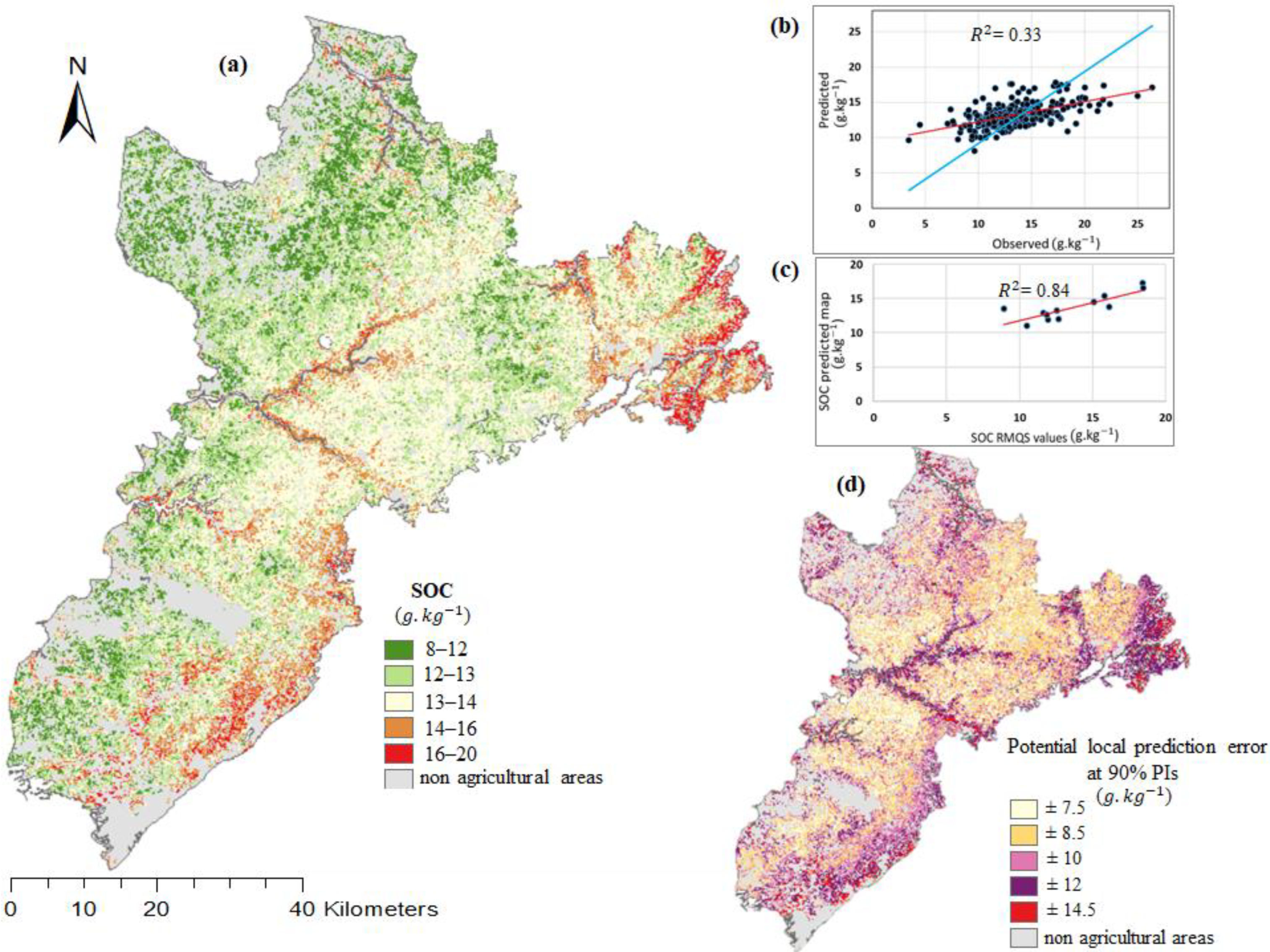
• Vaudour et al. [22] reported better performance in predicting SOC when soils with mean volumetric water content values higher than 25 vol.% were excluded. In order to eliminate highly wet soils, we chose S2 images using as criteria the mean pixel values of SMPs (<20 vol.%) for each date. In total, 57 S2 images were considered for the next step, and the LPIS was used to mask all non-agricultural sites (Figure 2a).
• A geophysical mask was used to remove clouds and/or topographic shadows and/or snow cover in each single-date S2 image (“masque géophysique” or MG2) [45]; this mask is available for all S2 images that can be downloaded from the Theia website.
• NDVI (Normalized Difference Vegetation Index) and NBR2 (Normalized Burn Ratio 2) were calculated to mask the vegetated (or covered by crop residues) pixels. Following some previous studies [19,22], we considered bare soil NDVI values between 0 and 0.30, and the values above were flagged as NA. NBR2 values > 0.175 were marked as NA to exclude sites covered by straw or crop residues. Castaldi et al. [14] reported that the most suitable threshold for good performance in SOC prediction models was considering NBR2 index values up to 0.175. At this point, 57 single-date images of bare soil were obtained.
• Finally, we calculated the median reflectance of all the images to obtain S2Bsoil.

According to previous studies [16,19,22], climatic conditions, soil physical conditions and maximum bare soil coverage (conditioning the sample size) influence the digital mapping performance of soil organic carbon. In this sense, we selected all 57 images and separated them by subsemester to evaluate two periods where soil conditions vary by crop rotation and management practices as well as seasonal changes: “late winter–spring” and “summer–autumn”. These two periods were chosen because they correspond to the maximum number of bare soils linked to winter crops (mainly wheat) and summer crops (mainly maize, sugar beet and sunflower) cultivated in this region. Therefore, we obtained an S2Bsoil image based on all the images (S2Bsoil_0), one using the images between February and May (25 bare soil images) (S2Bsoil_1) and another from the images between July and November (32 bare soil images) (S2Bsoil_2) over a 6-year period (Figure 2a).

2.5. Environmental Covariates

The covariates used in this study are listed in

Table 1. Environmental covariates are used as predictors for digital soil mapping.

Variable	Number	Scale/ Resolution	Expression a	Reference
Remote sensing
S2Bsoil_0 b	10	25 m		This study
S2Bsoil_1 b	10	25 m		This study
S2Bsoil_2 b	10	25 m		This study
SM_0 c	1	25 m		This study
SM_1 c	1	25 m		This study
SM_2 c	1	25 m		This study
Hue Index (HI)	3	25 m	(2 × R − G − B)/(G − B)	Mathieu et al. [47]
Grain Size Index (GSI)	3	25 m	(R − B)/(R + G+B)	Xiao et al. [48]
Calcareous Sedimentary rocks (CalcI)	3	25 m	(SWIR 1 − G)/(SWIR 1 + G)	Boettinger et al. [49]
Saturation Index (SI)	3	25 m	(R − B)/(R + B)	Mathieu et al. [47]
Brightness Index (BI)	3	25 m	$\surd ($(R² + G² + B²)/3)	Escadafal. [50]
Coloration Index (CI)	3	25 m	(R − G)/(R + G)	Pouget et al. [51]
Carbonate Index (CaI)	3	25 m	R/G	Boettinger et al. [49]
Geological response (Geol)	3	25 m	(SWIR 1 − SWIR 2)/(SWIR 1 + SWIR 2)	Nield et al. [52]
First three PCs of NDVI S2Bsoil d	9	25 m		This study
First three PCs of monthly MODIS NDVI d	3	500,300 m		Loiseau et al. [25]
Topography and position
Elevation	4	25 m		IGN [53]; Chen et al. [54]
Slope	4	25 m		IGN [53]; Chen et al. [54]
Slope position (PS)	4	25 m		IGN [53]; Chen et al. [54]
Slope length (LS)	4	25 m		IGN [53]; Chen et al. [54]
Terrain wetness index (TWI)	4	25 m		IGN [53]; Chen et al. [54]
Valley depth (VD)	4	25 m		IGN [53]; Chen et al. [54]
Vertical distance to channel network (VDCN)	4	25 m		IGN [53]; Chen et al. [54]
Multiresolution index of valley bottom flatness (MrVBF)	4	25 m		IGN [53]; Chen et al. [54]
Channel network base level (CNBL)	4	25 m		IGN [53]; Chen et al. [54]
Plan curvature	4	25 m		IGN [53]; Chen et al. [54]
Profile curvature	4	25 m		IGN [53]; Chen et al. [54]
Coordinates (Latitude, Longitude)	2	25 m
Oblique coordinates (OC) e	10	25 m		Chen et al. [54]; Møller et al. [55]
Parent material
Parent material	1	1:1 M		King et al. [56]
Gamma ray (K, U, Th, TC)	4	250 m		Martelet et al. [37]

^a R: Red; G: Green; B: Blue; SWIR1: short-wave infrared1; SWIR2: short-wave infrared2. ^b S2Bsoil (0,1,2): Sentinel-2 temporal mosaics of bare soil images. ^c SM (0,1,2): soil moisture product means calculated for the same dates as S2Bsoil (0,1,2). ^d PCs, principal components; NDVI, normalized difference vegetation index. ^e Oblique coordinates at angles of 15°, 30°, 45°, 60°, 75°, 105°, 120°, 135°, 150° and 165°.

, separated into remote sensing data, topography, position and parent material. We used these covariates based on the main environmental factors of the scorpan model that may control the variability of the SOC proposed by McBratney et al. [5]. The resolution and scales of the environmental covariates were different. Therefore, we harmonized them to a 25-m resolution using the nearest neighbor method for spatial predictive modeling and mapping at non-visited locations. In addition, the nearZeroVar function of the caret package [46] in R (R Core Team, 2020) was used to remove covariates with zero or near-zero variance (Figure 2b).

2.5.1. Remote Sensing

The 10 bands of the three S2Bsoil were used, and SMPs pixelwise means were calculated considering the same bare soil mosaic periods: using all images (SM_0), between February and May (SM_1) and between July and November (SM_2). Several spectral indices related to parent material and soil were derived from the bands of the three S2Bsoil. Table 1 provides more details on the 8 indices calculated from the S2 spectral bands for each mosaic.

NDVI by single date was used in this study; the 57 NDVI dates were collected and reduced to the first three principal components (PCs) (keeping the same periods of the S2Bsoil) by principal component analysis (PCA) to eliminate their multicollinearity. We chose to use PCA under the assumption that the sensitivity of spectral indices such as NDVI to SOC and soil texture is linked to different soil types and parent materials [15,57]. In addition, the use of PCA applied to the NDVI time series has shown the potential to identify seasonal changes in land cover [58]. We also included the three PCs of 24 monthly NDVI data in 2003 (an extremely warm and dry year) and 2016 (a normal year) acquired from MODIS (500 m resolution) and the PROBA-V 10-day product level 2B TOC (300 m resolution). For more details, we refer to Loiseau et al. [25].

2.5.2. Topography and Position

The Digital Elevation Model (DEM) of mainland France (25 m resolution) derived from the BD TOPO 3 of the French National Geographic Institute [53] was used. The covariates derived from the DEM were computed in the SAGA GIS Channels Library [59] (Table 1). According to McBratney et al. [5], neighboring locations on the topography can provide useful information in soil modeling. Grinand et al. [60] and Loiseau et al. [25] investigated the potential of incorporating local neighborhood information into training pixels using convolution filtering operations to predict soil class distribution and clay content, respectively. In a recent study, Chen et al. [54] used mean convolution circular windows to calculate the focal means to map the soil thickness of loess deposits in our study area. We, therefore, included the focal means of topography covariates with radius at 200, 500 and 1000 m, which were produced earlier. For more details, we refer to Chen et al. [54]. Finally, the position covariates (latitude and longitude) extracted for each recorded pixel were used for modeling. In addition, 10 oblique geographic coordinates (OGC) at angles of 15°, 30°, 45°, 60°, 75°, 105°, 120°, 135°, 150° and 165° computed by Chen et al. [54] were included as covariates.

2.5.3. Parent Material

The parent material raster was obtained from the French national parent material map [56]. Alluvial deposits, clayey materials and sandy materials are present in the study area. However, calcareous rocks and loamy materials are the most common parent materials (42 and 49% of the area, respectively) (Figure 2b). Parent material was also characterized by means of airborne gamma-ray spectrometry, which measures the emission of three naturally occurring elements that have radioisotopes with sufficient energy and intensity to be measured from the air: uranium (U), thorium (Th) and potassium (K) [61]. K is measured directly through the isotope 40 K, whereas 232 Th and 238 U are measured through their radioactive daughters (208 Tl and 214 Bi, respectively). These emissions capture information from the upper 50 cm of the soil/rocks that is related to their geochemical composition, mineralogy and weathering. The gamma-ray data (K, Th, U) and total count (TC) used in this study were acquired by an airborne high-resolution magnetic and radiometric survey over the Région Centre by Terraquest Ltd. Canada, under the supervision of the BRGM [37]. The survey was conducted during the autumn and winter of 2008–2009. In order to minimize the effects of soil moisture from rainfall on gamma-ray emissions during rainy days, the measurements were interrupted for several hours after rainfall. The footprint of each measurement is an ellipse of approximately 150 × 300 m² and the data were interpolated using a standard minimum curvature interpolation on 250 m grids. Gamma-ray emissions being presumably stable over the time span since the airborne acquisition, there was no need to match Sentinel-2 data.

2.6. Datasets for Modeling

The flowchart in Figure 2c summarizes that before SOC modeling (see Section 2.7), we focused on the bare soil mosaics elaborated in Section 2.4. First, we extracted the band values of all S2Bsoil and other covariates (Table 1) and obtained our regression matrix. Then, the set of covariates was divided into 4 sets for each S2Bsoil:

-

M1, the bare soil reflectance of the 10 S2Bsoil bands was used (10 covariates);

-

M2, the 10 S2Bsoil bands plus spectral indices were considered (24 covariates);

-

M3, the same covariates used in M2 and soil moisture were used (25 covariates);

-

M4, all covariates used in the previous models plus covariates of topography, position and parent material were integrated (85 covariates).

Note that for each S2Bsoil, we obtained four different models, i.e., sixteen models in total were run.

2.7. Quantile Regression Forest and Model Performance Evaluation for SOC Prediction

The challenge of producing more accurate and robust digital soil property maps has driven the use of several machine learning models. Quantile regression forest (QRF, Meinshausen, [62]), based on the random forest model (RF, Breiman, [63]), has been largely used at regional and national scales [25,54,64,65,66]. Therefore, QRF was used to model SOC in this study (Figure 2c).

The QRF algorithm estimates a large set of bootstrap trees by randomly sampling n independent observations. For each node of a bootstrap tree, several dependent variables (covariates) are randomly sampled to split the observations. For all decision nodes, QRF, in contrast to RF, keeps the value of all observations, not just their mean, as RF does. In addition, based on an analysis of the conditional distribution based on the stored information, the prediction intervals are calculated.

We used the package quantregForest [67] in R version 4.2.0 for implementing QRF to derive the median prediction (50% quantile) and 90% prediction intervals (PIs, 5% and 95% quantiles). In order to obtain comparable and robust statistics, we optimized the selection of observations from the dataset in each model (see Section 2.6.) by 10-fold cross-validation with the caret package [46] in R [68]. Ten models were generated by selecting a different calibration and validation set each time. This process was repeated 5 times, i.e., 50 repeated models were obtained. QRF is often described as a method that is not very sensitive to overfitting. However, this is not completely true. The repeated k-fold cross-validation avoids putting all the samples in model fitting and allows for control a posteriori if over-fitting occurs (i.e., if learning performances are much better than validation performances). A basic rule to avoid overfitting consists of putting in the learning covariates set covariates that have a real soil process meaning. More sophisticated selections of covariates, such as recursive feature elimination [69] or the Boruta algorithm [70] exist, but they are often used when the set of covariates is very large and/or redundant. We did not use these selections in this study.

The default number of trees (ntree = 500) and the minimum node size (nodsize = 5) were considered. The number of variables randomly sampled as candidates in each split (mtry) was set as the default (total number/3) for each model. The QRF includes the option to calculate the variable importance determined by the increased mean squared error (IncMSE, in %) between the model excluding and including a given variable [54]. Variable importance was calculated by averaging the 50 repeated models mentioned above. Performance was evaluated on the validation sets by the coefficient of determination (R², Equation (1)); root mean square error (RMSE, Equation (2)); bias (Equation (3)) and concordance (Equation (4)) [71].

$$R^2=1-\frac{\sqrt{{{\displaystyle \sum }}_{i=1}^n{\left(y_i-{\widehat{y}}_i\right)}^2}}{\sqrt{{{\displaystyle \sum }}_{i=1}^n{\left(y_i-\overline{y}\right)}^2}},$$

(1)

$$RMSE=\sqrt{{{\displaystyle \sum }}_{i=1}^n\frac{{\left(y_i-{\widehat{y}}_i\right)}^2}{n}},$$

(2)

$$bias={{\displaystyle \sum }}_{i=1}^n\frac{\left({\widehat{y}}_i-y_i\right)}{n},$$

(3)

$$Concordance=\frac{2*{{\displaystyle \sum }}_{i=1}^n\frac{\left(y_i-\overline{y}\right)*\left({\widehat{y}}_i-\mathsf{Ÿ}\right)}{n}}{{\sigma }_{y_i}^2+{\sigma }_{{\widehat{y}}_i}^2+{\left(\overline{y}-\mathsf{Ÿ}\right)}^2},$$

(4)

where n is the number of samples, $y_i$ and ${\widehat{y}}_i$ are the the observed value and the predicted value for sample i, $\overline{y}$ and $\mathsf{Ÿ}$ is the mean of the observed and predicted values; ${\sigma }_{y_i}^2$ and ${\sigma }_{{\widehat{y}}_i}^2$ are the observation and prediction variances.

After predictions and performance assessments, we selected, mapped and discussed the model approach that performed the best. The 90% PIs were used to display the local uncertainty of the SOC map. In addition, we used 12 independent soil samples from the French soil monitoring network (RMQS; Jolivet et al. [72]; Mulder et al. [9,73]) to evaluate the SOC values of the predicted map in agricultural plots regarding this monitoring network that extends across France in a 16 km × 16 km square grid sampling.

3. Results

In the following paragraphs, the three temporal bare soil mosaics (S2Bsoil_0, S2Bsoil_1, S2Bsoil_2) generated in this study are first presented. Subsequently, the SOC content prediction performance is presented according to the aforementioned mosaics, and the influence of the most important environmental covariates on the modeling is discussed. Lastly, a predicted top SOC content map (average predicted SOC values from the 50 models) at a 25 m resolution per pixel and its uncertainty are provided and analyzed.

3.1. Maximum Bare Topsoil Area Mapped and Description of Spectral Patterns

The mean percentage of bare soils on single dates between February and May was lower than the mean between July and November (~24% and ~41% of bare soil pixels, respectively) (Supplementary Material Tables S3 and S4). S2Bsoil_0, with 57 images considered, achieved the highest percentage of bare topsoil mapping (81.8%), followed by S2Bsoil_2 and S2Bsoil_1 (81.4% and 70.9%, respectively) (Figure 3). The difference between S2Bsoil_0 and S2Bsoil_2 (0.4%) showed that detecting a bare soil cover higher than 80% of the agricultural area was possible with a 32-date time series. Furthermore, we found that all S2Bsoil obtained an acceptable potential to recover bare soil pixels, confirmed by the closeness of the scattering points to the 1:1 soil line [74]. The coefficients of determination in the soil line analysis were high (R² > 0.8) (Figure 3); similar results were reported by Silvero et al. [17], who used Sentinel and Landsat images to extend the area of bare soil.

Table 2. SOC sample set statistics for each S2Bsoil used for modeling.

		SOC g.kg−1
S2Bsoil	Sites	Minimum	Q1	Median	Mean	Q3	Maximum	SD	Skewness	Kurtosis
S2Bsoil_0	353	3.46	11.40	13	13.4	15	27.8	3.34	0.86	4.83
S2Bsoil_1	304	3.46	11.41	13	13.4	15	27.8	3.32	0.93	5.18
S2Bsoil_2	350	3.46	11.39	13	13.4	15	27.8	3.35	0.85	4.82

Q1, the first quartile; Q3, the third quartile.

displays the statistics of SOC content in the Beauce area for the sites of each bare soil mosaic. As expected, due to their percentage of bare soil, S2Bsoil_0 and S2Bsoil_2 obtained the highest number of sites from our database (353 and 350 sites, respectively), while S2Bsoil_1 used 304. The statistics among the three sets were similar; SOC ranged from 3.5 to 27.8 g.kg⁻¹ (mean of 13.4 g.kg⁻¹; median of 13 g.kg⁻¹; standard deviation of three g.kg⁻¹). A skewness between 0.85 and 0.93 indicated that the data were positively but moderately skewed, while a kurtosis > three showed that the data had a heavy-tailed leptokurtic kurtosis. A logarithmic transformation was used to convert the data to a normal distribution; however, this did not improve the model’s performance. Therefore, we used the original SOC data for spatial modeling in this study.

Figure 4 shows for each bare soil mosaic (S2Bsoil_0, S2Bsoil_1 and S2Bsoil_2) the spectral patterns of median reflectance calculated from the quartile values of the SOC samples used for each S2Bsoil. As expected, the spectral features of the first quartiles (i.e., the lowest SOC content ≤ 11.4 g.kg⁻¹) showed the highest reflectance values, while the spectral features with the lowest reflectance corresponded to the quartiles with the highest SOC content. Generally, a difference between SOC quartiles was observed, confirming the quality of each mosaic. However, in S2Bsoil_1, such a difference was more noticeable, especially in quartiles three and four, whereas in S2Bsoil_0 and S2Bsoil_2, these two quartiles had quite similar values. The number of samples used for each bare soil mosaic in Figure 4 was lower than the number of samples mentioned in Section 2.1 (391 samples) because they were the only available samples located in bare soil pixels for each mosaic (S2bsoil). That is, as each S2Bsoil was elaborated with images in different periods, the bare soil pixels and their location varied, and then for each mosaic, the number of samples varied and was always lower than 391.

3.2. SOC Model Performance

The performance of the SOC content predictions varied according to the S2Bsoil and the environmental covariate datasets used. The best model performances were obtained using all covariates for each S2Bsoil (sets M4, e.g., 0.26 ≤ R² ≤ 0.33 and 2.59 g.kg⁻¹ ≤ RMSE ≤ 2.75 g.kg⁻¹) (

Table 3. Model performance of a Quantile Random Forest to predict soil organic carbon by mosaics of bare soil over a 6-year period (the values presented correspond to the mean values of the 50 repetitions mentioned in Section 2.7).

S2Bsoil	Modeling Dataset	R2	RMSE (g.kg−1)	Bias	Concordance
S2Bsoil_0	M1	0.18	3.00	−0.33	0.32
	M2	0.19	2.98	−0.31	0.33
	M3	0.15	2.98	−0.30	0.29
	M4	0.26	2.75	−0.20	0.40
S2Bsoil_1	M1	0.19	2.97	−0.32	0.35
	M2	0.22	2.90	−0.30	0.35
	M3	0.22	2.79	−0.28	0.34
	M4	0.33	2.59	−0.22	0.42
S2Bsoil_2	M1	0.11	3.17	−0.35	0.25
	M2	0.11	3.14	−0.30	0.24
	M3	0.12	3.00	−0.29	0.25
	M4	0.27	2.71	−0.21	0.39

R², coefficient of determination; RMSE, root mean square error.

). We obtained decreasing performances when only the S2 bands were considered. All M1 models exhibited the lowest performance, 0.11 ≤ R² ≤ 0.18, RMSE ≥ 2.97 g.kg⁻¹ and a maximum bias of −0.35 g.kg⁻¹. The performances of the models considering S2Bsoil_0 and S2Bsoil_2 showed a close result; however, the maximum RMSE reached (3.17 g.kg⁻¹) was obtained using only the set of spectral bands (M1) of the bare soil mosaic produced from S2 images between July and November (S2Bsoil_2). The poor performance of the S2BSoil_2 models may presumably be associated with the SM measured at each single date; the SMPs between July and November of our time series showed a slightly higher mean value (SM ≈ 13.9 vol.%) compared to those between February and May (SM ≈ 13.2 vol.%) for S2Bsoil_1 (Supplementary Material Figures S1 and S2). In addition, the inter-day difference (ds2–DSM) between SMPs and S2 images between July and November was higher with respect to the scenes considered between February and May, so it is possible that a bias of the real moisture values in the single dates of this particular period affected the modeling performance.

3.3. Influential Covariates

Figure 5 displays the top 25 environmental covariates in the computed QRF models. This figure compares three models for each temporal bare soil mosaic using the M4 dataset. The number of contributing covariates originating from remote sensing (satellite S2, S2 indices and SM in addition to gamma-ray) was 13 or 14 out of 25 for the temporal mosaics of all dates (S2Bsoil_0) or of “late winter–spring” dates (S2Bsoil_1), while that of topography and position was slightly higher (15) for the temporal mosaic of “summer–autumn” (S2Bsoil_2) only. It is worth noting that satellite and gamma-ray covariates prevailed in the top five influent covariates, whatever the S2 temporal mosaic, and that all S2 bands were among the influent covariates. The most significant bands among the best-performing models were from the near-infrared (b6, b7, b8 and b8a) and SWIR (b11, b12) regions, and, to a lesser extent, from the visible region through the CalcI index (b3). While all S2 bands turned out to be influent, only three out of eight soil spectral indices (CalcI, followed by BI and then HI) had a predictive weight for Beauce. The best temporal series was composed of “late winter–spring” dates when bare soil is not likely to be disturbed by crop residues; the S1-derived soil moisture appears influent using only this temporal mosaic, which makes sense noting the closeness of the dates between the S2 images with which S2Bsoil_1 was constructed and the SMPs mentioned above in Section 3.2.

Our results also indicate the fundamental role played by the information of neighboring distances of topography in the three models, particularly for the “summer–autumn” temporal mosaic: slope (with 200 m radius, SLOPE8), slope length (with 200 m radius, LS8), DEM (with 1000 m radius, DEM40) and MrVBF (with 1000 m radius, MRVBF40). The OGC at an angle of 135° (oblique135) was among the 25 most important covariates in all bare soil mosaics.

Furthermore, both thorium and uranium surface concentrations derived from airborne gamma-ray surveys also played an important role in the prediction of SOC, especially for S2Bsoil_2 and S2Bsoil_0. In DSM, gamma-ray spectrometry can be used as a substitute for lithological maps [75]. A recent review [76] pointed out the main applications of gamma rays in mapping some soil attributes (e.g., parent material, topsoil soil texture, clay mineralogy, weathering intensity and soil type). A strong limitation is that gamma-ray data are far from covering the whole world (and even the whole of France) because of their cost and because they have been mainly used for mining purposes. Although the use of airborne gamma-ray data in soil science has been mainly explored to assist digital soil mapping and to understand landscape processes, lithology and mineralogy [54,77,78], there are still a few papers that relate soil attributes to gamma radiation emissions at a rather broad scale [75,79,80,81]. Thorium is rather stable under conditions of soil at about or higher than pH seven, where it can be adsorbed to the surface of clay minerals and organic matter [82]. Note that under intensive cultivation and over calcareous bedrock, this is the case [83]. Therefore, it is not surprising that gamma-ray data emitted by thorium contributes to this study by predicting SOC. Note that in Figure 1, in the southeast of the study area, high SOC values are observed in the sampling sites and in Figure 2b, in the same part, the thorium image shows the highest values. This zone is characterized by the presence of soils with a clayey texture. An opposite effect is observed to the north on a large plateau with a deep loess thickness that was prone to a loss of clay content in topsoil by a process of illuviation [54]. In this area, the values of gamma radiation emitted by thorium are lower.

3.4. SOC Variability and Predicted Spatial Uncertainty

Figure 6a displays the predicted SOC map calculated from the S2Bsoil_1 bands and all covariates in the M4 data set. The mean and standard deviation of the predicted SOC content values were 13.2 g.kg⁻¹ and 1.6 g.kg⁻¹ respectively, i.e., quite similar to the mean and distribution of SOC observed values (Table 2 and Figure 1). The map of SOC clearly exhibits some gradients in SOC distribution. These gradients depict some general trends that could be linked to relationships between clay and SOC content [84] (Supplementary Material Figure S3). Indeed, the northern area, which is highly depleted in clay due to illuviation, has very low SOC contents. This area corresponds to a wide loessic plateau already identified by Chen et al. [54] when studying the thickness of loess in the same region. The effect of local topography is also very striking, with numerous high values close to the valleys.

Note, however, that the validation results are far from the 1:1 line (Figure 6b). In other words, there is a general tendency to overestimate the low SOC values and underestimate the high ones. The low sample density of higher and lower SOC values in our set (Figure 1) might have influenced the prediction accuracy at the extreme values in the modeling. Note also that the same trend is observed for the 12 points of the systematic independent grid (Figure 6c).

The remote sensing data and covariates used in our model were significant in mapping mainly mean SOC values in mid-elevation areas to lower values in flat areas over plateaus at high elevation (Figure 6d). Nevertheless, 90% prediction intervals were large. The wind direction of the loess deposits observed mainly in the large plateau to the north was from the northwest [54,85,86] and interestingly, one of the most important covariates was oblique135. Figure 7a shows this covariate divided into four classes. Dividing our predicted SOC map and thorium gamma image into the same classes provides striking matching (Figure 7b,c, respectively), in which a trend from lower SOC and thorium values from the northwest to higher values towards the southwest is observed.

4. Discussion

Over an intensively managed agricultural region such as Beauce, the SOC content of the top horizon is rather low with a narrow range of values, which hampers a good prediction using only spectral optical models [20,87], and indeed, the use of a more diversified and relevant set of covariates enabled the best-performing model to be reached. This study demonstrates that it is worthwhile to include temporal mosaics of bare soils in such a DSM approach, especially in conjunction with airborne gamma-ray and morphometric data.

4.1. The More Relevant Set of Covariates in SOC Modeling

4.1.1. The Importance of Both Satellite-Derived and Morphometric Covariates in SOC Modelling

Previous studies have reported that the importance of S2 bands for predicting SOC can vary depending on the study area and soil conditions during the date of image acquisition [15,19,20,88,89]. Similar results about the importance of the S2 bands of a temporal mosaic of bare soil were found by Žížala et al. [21], but these authors did not include spectral indices as covariates.

Behrens et al. [90] stated that spatial context influences the content of soil attributes when considering long-range processes (teleconnected systems). These authors suggested that including covariates derived from multi-scale neighboring information can enable the identification of spatial trends in the data using machine learning models to improve their accuracy. In our case, the importance of slope and MrVBF might be related to a long-range effect from lower SOC values at high-elevation plateaus, medium values at mid-elevation locations and a higher increase at steep slopes surrounding valleys, mainly near rivers. Previous studies have shown promising results on the performance of models including covariates of neighboring information in DSM [54,91]. Recently, in a national-scale SOC mapping, Žížala et al. [21] used a mixed approach of octave formation (Gaussian pyramids) for relief covariates and reported multi-scale derivatives of elevation among the most important covariates. Another method to fill the gap with respect to the ability to identify spatial trends over large regions that enable the estimation of soil attributes using Random Forest is the calculation of OGC that are used as covariates [55]. The use of OGC (specifically, “oblique135”) in Beauce confirms the results obtained by Møller et al. [55], who reported in an agricultural field in Denmark that including OGC contributes to the prediction of organic matter due to the ability of these to identify from terrain features to management practices in a geographic space.

4.1.2. The Major Importance of Airborne Gamma-Ray Covariates in SOC Modelling

Interestingly, our results emphasize the importance that airborne gamma-ray data plays in SOC modeling. Our results confirm an indirect relationship between gamma-ray emissions and SOC. This confirms the results of Dierke and Werban [92], who stated at a field site that it is possible to indirectly estimate organic carbon through thorium concentrations. In a nearby region of France, Loiseau et al. [75] demonstrated that thorium was among the most important co-variates to predict clay content. Therefore, in soils that have been cultivated for many decades, it cannot be excluded that a large proportion of the remaining SOC in topsoil is controlled by stabilization by clay [84,93,94]. Indeed, we observed a positive relationship between clay and SOC content in the Beauce French topsoil used in this study for plots for which both parameters were measured (Supplementary Material Figure S2).

The results obtained with uranium are more difficult to explain since the behavior of uranium in soils is quite complex. Uranium is fairly mobile and may significantly vary according to soil physicochemical conditions; in particular, the redox state and saturation of soils play an important role in the adsorption of uranium on clays and organic matter. It is, however, difficult to relate U and SM contents since dedicated acquisition methodology and processing are applied to reduce as much as possible the effect of soil moisture on gamma-ray data [95]. Lastly, despite specific corrections taken in the preprocessing of gamma-ray data [96], the presence of radon gas in the disintegration chain of uranium also complicates the reading of this variable. The relationship between SOC and uranium content in soils is, however, well evidenced in our study, and further specific analysis would be needed to clearly explain this relationship.

4.2. SOC Variability and Predicted Spatial Uncertainty

The validation by the 12-point grid should be taken with caution because it has been demonstrated that using a very small number of independent sites may lead to erroneous conclusions [64]. Large 90% prediction intervals are rather common for DSM SOC prediction at such resolution and over a rather wide area [97]. It is quite likely that the uncertainty could be traced to the underestimation of the extreme values mentioned above. In our study, it was very difficult to establish one main reason that impacts the confidence level of prediction at sites with higher uncertainty. Still, management practices in agricultural plots, topography, soil physical conditions and historical soil-forming environmental processes in Beauce may influence SOC content and its detection via satellite [16,19,32,55]. The SOC gradient that we observed along the study area might be influenced in some way by the direction of the winds that deposited the loess. In other words, considering OGC, it was possible to detect a spatial trend related to the SOC content [55].

4.3. Perspectives for SOC Mapping over Large Agricultural Regions

The availability of satellite imagery at no cost (e.g., Sentinel and Landsat) has been a turning point that has driven the use of remote sensing-derived techniques and products in soil science for bare soil retrieval, attribute mapping and quantification (e.g., SCMaP, Rogge et al. [98]; GEOS3, Demattê et al. [23]; HISET, Heiden et al. [99]; R90, Castaldi et al. 2023 [89]; moisture maps, El Hajj et al. [40]). The development of these products enables us to obtain information about the soil surface (e.g., soil moisture maps) and to extend the percentage of bare soil. This last point is, however, questionable, as cover cropping is more and more recommended to increase SOC inputs in soils and favor SOC sequestration. This is one paradox of science for SOC remote sensing: bare soils favor better detection of SOC by remote sensing, but practices recommended to increase SOC include having soils continuously covered by vegetation. Our results obtained by evaluating S2Bsoil in two different periods of the year demonstrate that a given period, here the “late winter–spring” for Beauce, significantly favors the performance of topsoil prediction by DSM at the regional scale while including different covariates in the modeling such as airborne gamma-ray data, DEM derivatives and coordinates. The uncertainty, however, remained quite high, which raises questions about the feasibility of transitioning from mapping to monitoring over short-term time ranges. An important finding in this study was the observation of a spectral trend in neighboring pixel information in the entire region related to natural soil-forming processes. However, although SOC detection using spectral information from satellite images has grown exponentially in the last 5 years, mainly in farms and small regions (areas with a median of 118 km²) [87], there are still few studies for large agricultural regions that describe such trends in cultivated areas.

Previous studies in small regions reported that soil surface condition (e.g., SM, soil roughness, plant residues) and hence the date of image acquisition should be considered as one of the main factors impacting SOC retrieval via satellite [14,16,89]. Therefore, increasing the number of soil surface condition variables for a single date or time series to be used as input covariates in models should be further explored in large agricultural regions. Temporal images of soil moisture are becoming available and are constantly being improved [40,41], while soil roughness products are still very limited and barely tested in small regions [100]. Information about land use history could also be interesting, but such information is much more tedious to gather at the scale of a region as large as Beauce. This information could have been crucial if some drastic changes in land use had happened in recent decades (e.g., deforestation), but the Beauce region has been cultivated for a very long time. It is important to note that a large number of covariates providing information on soil surface conditions might not necessarily improve modeling performance but may be useful information to identify factors influencing SOC detection. Our results suggest that some additional co-variates could be useful, such as clay content maps. However, we should keep in mind that these maps are also not error-free and that adding them as co-variates may induce some more error propagation. However, the continuous accumulation of soil data through ongoing French and EU programs will progressively help to obtain more and more precise maps and data for monitoring.

Regional models often require more in-depth study than on-farm or small-region models due to the short time step of SOC variability influenced by climate, landforms, parent material, management practices and crop rotation [19,22]. Obviously, we also missed some information about long-term soil management and carbon inputs to the soil in the past, such as the application of EOM as an amendment to increase the productivity of agricultural soils [31]. Green waste compost and manure application change SOC content as well as the spectral information detected by the satellite. These increasingly common practices are driving studies that aim to develop spectral indices in agricultural plots capable of detecting whether or not there was any application of any type of soil amendment [32,101]. Therefore, further studies could include this information as a tool for increasing performance in SOC prediction in wide regions where these types of practices may be present. Obtaining information on agricultural practices, crop yields and SOC inputs thanks to remote sensing is, for sure, a key input for SOC modeling, mapping and forecasting.

5. Conclusions

This study was conducted over a large area of intensive agriculture to evaluate the Sentinel-2 satellite’s ability to predict SOC. Our approach was based on bare soil areas from temporal mosaics (S2Bsoil) over a 6-year period. Although the maximum bare soil coverage (81.8%) was reached using a series of 57 single dates, the performance for predicting SOC was not the best. The use of S2Bsoil by periods considering management practices and activities related to crop rotation (e.g., soil seedbed condition at the end of winter and potentially high presence of straw after harvest in late summer) slightly showed a difference in the accuracy of the models. Therefore, it is worth taking into account the soil management practices in a given region prior to building temporal bare soil mosaics over long time series to map SOC. We highlight that the use of SMPs is a valuable tool that helps to choose the best dates to create temporal bare soil mosaics; however, the SMPs uncertainty associated with the days of difference between the study dates and the products may induce biases, leading to an increase in SOC prediction uncertainty.

The relative importance of environmental covariates indicated the weight of S2 bands jointly with airborne gamma-ray imagery and morphometric covariates in the SOC modeling of the top horizon. Topography neighbor distances, OGC and gamma thorium were also key covariates in this study for their contribution not only to SOC mapping but also to providing information related to the impact of long-range effects on SOC content in such a specific region.

The produced SOC map makes sense from a topographical and historical perspective related to past natural processes and the intense agricultural activity present for decades in the area. This map can be used in soil management decision-making from a global perspective in Beauce. However, for farmers, i.e., at a local farm scale, the uncertainty map shows that more detailed studies would be required. Further studies might use this information to better locate new soil sampling efforts and reduce the error. Surveys of farmers’ practices would be a useful tool to identify management practices, such as organic amendments, that could distort SOC prediction at the local scale. Conversely, methods to produce variables from neighboring information might be useful in regional-scale machine learning models in order to better detect broad spatial trends related to SOC variability.

References

1. Ramankutty, N.; Evan, A.T.; Monfreda, C.; Foley, J.A. Farming the planet: 1. Geographic distribution of global agricultural lands in the year 2000. Glob. Biogeochem. Cycles 2008, 22, 1–19. [Google Scholar] [CrossRef]
2. Lal, R. Carbon sequestration. Philos. Trans. R. Soc. B Biol. Sci. 2008, 363, 815–830. [Google Scholar] [CrossRef]
3. Paustian, K.; Lehmann, J.; Ogle, S.; Reay, D.; Robertson, G.P.; Smith, P. Climate-smart soils. Nature 2016, 532, 49–57. [Google Scholar] [CrossRef]
4. Minasny, B.; Malone, B.P.; McBratney, A.B.; Angers, D.A.; Arrouays, D.; Chambers, A.; Chaplot, V.; Chen, Z.S.; Cheng, K.; Das, B.S.; et al. Soil carbon 4 per mille. Geoderma 2017, 292, 59–86. [Google Scholar] [CrossRef]
5. McBratney, A.B.; Mendonça Santos, M.L.; Minasny, B. On digital soil mapping. Geoderma 2003, 117, 3–52. [Google Scholar] [CrossRef]
6. Hengl, T.; De Jesus, J.M.; Heuvelink, G.B.M.; Gonzalez, M.R.; Kilibarda, M.; Blagotić, A.; Shangguan, W.; Wright, M.N.; Geng, X.; Bauer-Marschallinger, B.; et al. SoilGrids250m: Global gridded soil information based on machine learning. PLoS ONE 2017, 12, e0169748. [Google Scholar] [CrossRef]
7. Poggio, L.; De Sousa, L.M.; Batjes, N.H.; Heuvelink, G.B.M.; Kempen, B.; Ribeiro, E.; Rossiter, D. SoilGrids 2.0: Producing soil information for the globe with quantified spatial uncertainty. Soil 2021, 7, 217–240. [Google Scholar] [CrossRef]
8. Arrouays, D.; Grundy, M.G.; Hartemink, A.E.; Hempel, J.W.; Heuvelink, G.B.M.; Hong, S.Y.; Lagacherie, P.; Lelyk, G.; McBratney, A.B.; McKenzie, N.J.; et al. GlobalSoilMap. Toward a Fine-Resolution Global Grid of Soil Properties. Adv. Agron. 2014, 125, 93–134. [Google Scholar] [CrossRef]
9. Mulder, V.L.; Lacoste, M.; Richer-de-Forges, A.C.; Arrouays, D. GlobalSoilMap France: High-resolution spatial modelling the soils of France up to two meter depth. Sci. Total Environ. 2016, 573, 1352–1369. [Google Scholar] [CrossRef] [PubMed]
10. Sanchez, P.A.; Ahamed, S.; Carré, F.; Hartemink, A.E.; Hempel, J.; Huising, J.; Lagacherie, P.; McBratney, A.B.; McKenzie, N.J.; De Lourdes Mendonça-Santos, M.; et al. Digital soil map of the world. Science 2009, 325, 680–681. [Google Scholar] [CrossRef]
11. Chen, S.; Arrouays, D.; Mulder, V.L.; Poggio, L.; Minasny, B.; Roudier, P.; Libohova, Z.; Lagacherie, P.; Shi, Z.; Hannam, J.; et al. Digital mapping of GlobalSoilMap soil properties at a broad scale: A review. Geoderma 2022, 409, 115567. [Google Scholar] [CrossRef]
12. Vaudour, E.; Bel, L.; Gilliot, J.M.; Coquet, Y.; Hadjar, D.; Cambier, P.; Michelin, J.; Houot, S. Potential of SPOT Multispectral Satellite Images for Mapping Topsoil Organic Carbon Content over Peri-Urban Croplands. Soil Sci. Soc. Am. J. 2013, 77, 2122–2139. [Google Scholar] [CrossRef]
13. Nanni, M.R.; Demattê, J.A.M. Spectral Reflectance Methodology in Comparison to Traditional Soil Analysis. Soil Sci. Soc. Am. J. 2006, 70, 393–407. [Google Scholar] [CrossRef]
14. Castaldi, F.; Chabrillat, S.; Don, A.; van Wesemael, B. Soil organic carbon mapping using LUCAS topsoil database and Sentinel-2 data: An approach to reduce soil moisture and crop residue effects. Remote Sens. 2019, 11, 2121. [Google Scholar] [CrossRef]
15. Gholizadeh, A.; Žižala, D.; Saberioon, M.; Borůvka, L. Soil organic carbon and texture retrieving and mapping using proximal, airborne and Sentinel-2 spectral imaging. Remote Sens. Environ. 2018, 218, 89–103. [Google Scholar] [CrossRef]
16. Vaudour, E.; Gomez, C.; Loiseau, T.; Baghdadi, N.; Loubet, B.; Arrouays, D.; Ali, L.; Lagacherie, P. The impact of acquisition date on the prediction performance of topsoil organic carbon from Sentinel-2 for croplands. Remote Sens. 2019, 11, 2143. [Google Scholar] [CrossRef]
17. Silvero, N.E.Q.; Demattê, J.A.M.; Amorim, M.T.A.; dos Santos, N.V.; Rizzo, R.; Safanelli, J.L.; Poppiel, R.R.; Mendes, W.d.S.; Bonfatti, B.R. Soil variability and quantification based on Sentinel-2 and Landsat-8 bare soil images: A comparison. Remote Sens. Environ. 2021, 252, 112117. [Google Scholar] [CrossRef]
18. Dvorakova, K.; Heiden, U.; Van Wesemael, B. Sentinel-2 exposed soil composite for soil organic carbon prediction. Remote Sens. 2021, 13, 1791. [Google Scholar] [CrossRef]
19. Urbina-Salazar, D.; Vaudour, E.; Baghdadi, N.; Ceschia, E.; Richer-De-forges, A.C.; Lehmann, S.; Arrouays, D. Using sentinel-2 images for soil organic carbon content mapping in croplands of southwestern france. The usefulness of sentinel-1/2 derived moisture maps and mismatches between sentinel images and sampling dates. Remote Sens. 2021, 13, 5115. [Google Scholar] [CrossRef]
20. Vaudour, E.; Gomez, C.; Fouad, Y.; Lagacherie, P. Sentinel-2 image capacities to predict common topsoil properties of temperate and Mediterranean agroecosystems. Remote Sens. Environ. 2019, 223, 21–33. [Google Scholar] [CrossRef]
21. Žížala, D.; Minařík, R.; Skála, J.; Beitlerová, H.; Juřicová, A.; Reyes Rojas, J.; Penížek, V.; Zádorová, T. High-resolution agriculture soil property maps from digital soil mapping methods, Czech Republic. CATENA 2022, 212, 106024. [Google Scholar] [CrossRef]
22. Vaudour, E.; Gomez, C.; Lagacherie, P.; Loiseau, T.; Baghdadi, N.; Urbina-Salazar, D.; Loubet, B.; Arrouays, D. Temporal mosaicking approaches of Sentinel-2 images for extending topsoil organic carbon content mapping in croplands. Int. J. Appl. Earth Obs. Geoinf. 2021, 96, 102277. [Google Scholar] [CrossRef]
23. Demattê, J.A.M.; Fongaro, C.T.; Rizzo, R.; Safanelli, J.L. Geospatial Soil Sensing System (GEOS3): A powerful data mining procedure to retrieve soil spectral reflectance from satellite images. Remote Sens. Environ. 2018, 212, 161–175. [Google Scholar] [CrossRef]
24. Diek, S.; Fornallaz, F.; Schaepman, M.E.; de Jong, R. Barest Pixel Composite for agricultural areas using landsat time series. Remote Sens. 2017, 9, 1245. [Google Scholar] [CrossRef]
25. Loiseau, T.; Chen, S.; Mulder, V.L.; Román Dobarco, M.; Richer-de-Forges, A.C.; Lehmann, S.; Bourennane, H.; Saby, N.P.A.; Martin, M.P.; Vaudour, E.; et al. Satellite data integration for soil clay content modelling at a national scale. Int. J. Appl. Earth Obs. Geoinf. 2019, 82, 101905. [Google Scholar] [CrossRef]
26. Viel, E. Etude des Processus de Transport des Solutés Hors Equilibre Physique: Application à la Zone non Saturée des Calcaires de Beauce. Ph.D. Thesis, University of Orleans, Orléans, France, 2016. [Google Scholar]
27. Macaire, J.M. Etude Sédimentologique des Formations Superficielles sur le Tracé de L’autoroute A10 Entre Artenay et Meung sur Loire. Ph.D. Thesis, University of Orleans, Orléans, France, 1971. [Google Scholar]
28. Le Bissonnais, Y.; Arrouays, D. Aggregate stability and assessment of soil crustability and erodibility: II. Application to humic loamy soils with various organic carbon contents. Eur. J. Soil Sci. 1997, 48, 39–48. [Google Scholar] [CrossRef]
29. Dexter, A.R.; Richard, G.; Arrouays, D.; Czyz, E.A.; Jolivet, C.; Duval, O. Complexed organic matter controls soil physical properties. Geoderma 2008, 144, 620–627. [Google Scholar] [CrossRef]
30. Lal, R. Carbon management in agricultural soils. Mitig. Adapt. Strateg. Glob. Chang. 2007, 12, 303–322. [Google Scholar] [CrossRef]
31. Moinard, V.; Levavasseur, F.; Houot, S. Current and potential recycling of exogenous organic matter as fertilizers and amendments in a French peri-urban territory. Resour. Conserv. Recycl. 2021, 169, 105523. [Google Scholar] [CrossRef]
32. Dodin, M.; Smith, H.D.; Levavasseur, F.; Hadjar, D.; Houot, S.; Vaudour, E. Potential of sentinel-2 satellite images for monitoring green waste compost and manure amendments in temperate cropland. Remote Sens. 2021, 13, 1616. [Google Scholar] [CrossRef]
33. Bouarfa, S.; Brunel, L.; Granier, J.; Mailhol, J.C.; Morardet, S.; Ruelle, P. Évaluation en partenariat des stratégies d’irrigation en cas de restriction des prélèvements dans la nappe de Beauce (France). Cah. Agric. 2011, 20, 124–129. [Google Scholar] [CrossRef]
34. Verley, F. Lessons from twenty years of local volumetric groundwater management: The case of the Beauce Aquifer, Central France. In Sustainable Groundwater Management; Springer: Berlin/Heidelberg, Germany, 2020; pp. 93–108. [Google Scholar] [CrossRef]
35. Paroissien, J.; Saby, N.; de Forges, A.; Arrouays, D.; Louis, B. Populating soil maps with legacy data from a soil testing databases. In GlobalSoilMap: Basis of the Global Spatial Soil Information System; Taylor & Francis, CRC Press: London, UK, 2014; pp. 319–324. [Google Scholar]
36. IUSS Working Group WRB. World Reference Base for Soil Resources 2014, Update 2015 International Soil Classification System for Naming Soils and Creating Legends for Soil Maps; FAO: Rome, Italy, 2015. [Google Scholar]
37. Martelet, G.; Nehlig, P.; Arrouays, D.; Messner, F.; Tourlière, B.; Laroche, B.; Deparis, J.; Saby, N.; Richer-de-Forges, A.C.; Jolivet, C.; et al. Airborne gamma-ray spectrometry: Potential for regolith-soil mapping and characterization. In GlobalSoilMap: Basis of the Global Spatial Soil Information System; Taylor & Francis, CRC Press: London, UK, 2014; pp. 401–408. [Google Scholar]
38. Arrouays, D.; Richer-de-Forges, A.C.; Héliès, F.; Mulder, V.L.; Saby, N.P.A.; Chen, S.; Martin, M.P.; Román Dobarco, M.; Follain, S.; Jolivet, C.; et al. Impacts of national scale digital soil mapping programs in France. Geoderma Reg. 2020, 23, e00337. [Google Scholar] [CrossRef]
39. Jones, A.; Fernandez Ugalde, O.; Scarpa, S. LUCAS 2015 Topsoil Survey; Publications Office of the European Union: Luxembourg, 2020. [Google Scholar] [CrossRef]
40. El Hajj, M.; Baghdadi, N.; Zribi, M.; Bazzi, H. Synergic use of Sentinel-1 and Sentinel-2 images for operational soil moisture mapping at high spatial resolution over agricultural areas. Remote Sens. 2017, 9, 1292. [Google Scholar] [CrossRef]
41. Bazzi, H.; Baghdadi, N.; El Hajj, M.; Zribi, M.; Belhouchette, H. A Comparison of Two Soil Moisture Products S2MP and Copernicus-SSM over Southern France. IEEE J. Sel. Top. Appl. Earth Obs. Remote Sens. 2019, 12, 3366–3375. [Google Scholar] [CrossRef]
42. Baghdadi, N.; El Hajj, M.; Zribi, M.; Bousbih, S. Calibration of the Water Cloud Model at C-Band for winter crop fields and grasslands. Remote Sens. 2017, 9, 969. [Google Scholar] [CrossRef]
43. Baghdadi, N.; Holah, N.; Zribi, M. Calibration of the Integral Equation Model for SAR data in C-band and HH and VV polarizations. Int. J. Remote Sens. 2006, 27, 805–816. [Google Scholar] [CrossRef]
44. Zepp, S.; Heiden, U.; Bachmann, M.; Wiesmeier, M.; Steininger, M.; van Wesemael, B. Estimation of soil organic carbon contents in croplands of bavaria from scmap soil reflectance composites. Remote Sens. 2021, 13, 3141. [Google Scholar] [CrossRef]
45. Baetens, L.; Desjardins, C.; Hagolle, O. Validation of copernicus Sentinel-2 cloud masks obtained from MAJA, Sen2Cor, and FMask processors using reference cloud masks generated with a supervised active learning procedure. Remote Sens. 2019, 11, 433. [Google Scholar] [CrossRef]
46. Kuhn, M. Caret: Classification and Regression Training. R Packag. Version 6.0-93. 2022. Available online: https://cran.r-project.org/web/packages/caret/index.html (accessed on 4 April 2023).
47. Mathieu, R.; Pouget, M.; Cervelle, B.; Escadafal, R. Relationships between Satellite-Based Radiometric Indices Simulated Using Laboratory Reflectance Data and Typic Soil Color of an Arid Environment. Remote Sens. Environ. 1998, 66, 17–28. [Google Scholar] [CrossRef]
48. Xiao, J.; Shen, Y.; Tateishi, R.; Bayaer, W. Development of topsoil grain size index for monitoring desertification in arid land using remote sensing. Int. J. Remote Sens. 2006, 27, 2411–2422. [Google Scholar] [CrossRef]
49. Boettinger, J.L.; Ramsey, R.D.; Bodily, J.M.; Cole, N.J.; Kienast-Brown, S.; Nield, S.J.; Saunders, A.M.; Stum, A.K. Landsat Spectral Data for Digital Soil Mapping. In Digital Soil Mapping with Limited Data; Hartemink, A.E., McBratney, A., Mendonça-Santos, M.d.L., Eds.; Springer: Dordrecht, The Netherlands, 2008; pp. 193–202. ISBN 978-1-4020-8591-8. [Google Scholar]
50. Escadafal, R. Remote Sensing of Arid Soil Surface Color with Landsat Thematic Mapper. Adv. Space Res. 1989, 9, 159–163. [Google Scholar] [CrossRef]
51. Pouget, M.; Madeira Netto, J.; Le Floc’h, E.; Kamal, S. Caractéristiques spectrales des surfaces sableuses de la région côtière Nord-Ouest de l’Egypte: Application aux données satellitaires SPOT. In Caractérisation et Suivi des Milieux Terrestres en Régions Arides et Tropicales; Pouget, M., Ed.; ORSTOM: Paris, France, 1991; pp. 27–38. ISBN 2-7099-1051-9. Available online: https://horizon.documentation.ird.fr/exl-doc/pleins_textes/pleins_textes_6/colloques2/34605.pdf (accessed on 4 April 2023).
52. Nield, S.J.; Boettinger, J.L.; Ramsey, R.D. Digitally Mapping Gypsic and Natric Soil Areas Using Landsat ETM Data. Soil Sci. Soc. Am. J. 2007, 71, 245–252. [Google Scholar] [CrossRef]
53. IGN. IGN (Institut Géographique National). 2011. Available online: https://geoservices.ign.fr/sites/default/files/2021-07/DC_BDALTI_2-0.pdf (accessed on 4 April 2023).
54. Chen, S.; Richer-de-Forges, A.C.; Leatitia Mulder, V.; Martelet, G.; Loiseau, T.; Lehmann, S.; Arrouays, D. Digital mapping of the soil thickness of loess deposits over a calcareous bedrock in central France. CATENA 2021, 198, 105062. [Google Scholar] [CrossRef]
55. Møller, A.; Beucher, A.M.; Pouladi, N.; Humlekrog Greve, M. Oblique geographic coordinates as covariates for digital soil mapping. Soil 2020, 6, 269–289. [Google Scholar] [CrossRef]
56. King, D.; Daroussin, J.; Tavernier, R. Development of a soil geographic database from the Soil Map of the European Communities. CATENA 1994, 21, 37–56. [Google Scholar] [CrossRef]
57. Demattê, J.A.M.; Sayão, V.M.; Rizzo, R.; Fongaro, C.T. Soil class and attribute dynamics and their relationship with natural vegetation based on satellite remote sensing. Geoderma 2017, 302, 39–51. [Google Scholar] [CrossRef]
58. Bellón, B.; Bégué, A.; Seen, D.L.; de Almeida, C.A.; Simões, M. A remote sensing approach for regional-scale mapping of agricultural land-use systems based on NDVI time series. Remote Sens. 2017, 9, 600. [Google Scholar] [CrossRef]
59. Conrad, O.; Bechtel, B.; Bock, M.; Dietrich, H.; Fischer, E.; Gerlitz, L.; Wehberg, J.; Wichmann, V.; Böhner, J. System for Automated Geoscientific Analyses (SAGA) v. 2.1.4. Geosci. Model Dev. 2015, 8, 1991–2007. [Google Scholar] [CrossRef]
60. Grinand, C.; Arrouays, D.; Laroche, B.; Martin, M.P. Extrapolating regional soil landscapes from an existing soil map: Sampling intensity, validation procedures, and integration of spatial context. Geoderma 2008, 143, 180–190. [Google Scholar] [CrossRef]
61. Minty, B. Fundamentals of airborne gamma-ray spectrometry. AGSO J. Aust. Geol. Geophys. 1997, 17, 39–50. [Google Scholar]
62. Meinshausen, N. Quantile regression forests. J. Mach. Learn. Res. 2006, 7, 983–999. [Google Scholar]
63. Breiman, L. Random Forests. Mach. Learn. 2001, 45, 5–32. [Google Scholar] [CrossRef]
64. Lagacherie, P.; Arrouays, D.; Bourennane, H.; Gomez, C.; Martin, M.; Saby, N.P.A. How far can the uncertainty on a Digital Soil Map be known? A numerical experiment using pseudo values of clay content obtained from Vis-SWIR hyperspectral imagery. Geoderma 2019, 337, 1320–1328. [Google Scholar] [CrossRef]
65. Lombardo, L.; Saia, S.; Schillaci, C.; Mai, P.M.; Huser, R. Modeling soil organic carbon with Quantile Regression: Dissecting predictors’ effects on carbon stocks. Geoderma 2018, 318, 148–159. [Google Scholar] [CrossRef]
66. Vaysse, K.; Lagacherie, P. Using quantile regression forest to estimate uncertainty of digital soil mapping products. Geoderma 2017, 291, 55–64. [Google Scholar] [CrossRef]
67. Meinshausen, N. QuantregForest: Quantile Regression Forests; Version 1.3-7. 2017. Available online: https://cran.r-project.org/web/packages/quantregForest/quantregForest.pdf (accessed on 4 April 2023).
68. R Core Team. R: A Language and Environment for Statistical Computing; R Foundation for Statistical Computing: Vienna, Austria, 2020. [Google Scholar]
69. Guyon, I.; Weston, J.; Barnhill, S.; Vapnik, V. Gene Selection for Cancer Classification using Support Vector Machines. Mach. Learn. 2002, 46, 389–422. Available online: https://link.springer.com/article/10.1023/A:1012487302797 (accessed on 4 April 2023). [CrossRef]
70. Kursa, M.B.; Rudnicki, W.R. Feature Selection with the Boruta Package. J. Stat. Softw. 2010, 36, 1–13. [Google Scholar] [CrossRef]
71. Lin, L.I.-K. A Concordance Correlation Coefficient to Evaluate Reproducibility. Biometrics 1989, 45, 255–268. [Google Scholar] [CrossRef]
72. Jolivet, C.; Arrouays, D.; Boulonne, L.; Ratié, C.; Saby, N. Le réseau de mesures de la qualité des sols de France (RMQS)-Etat d’avancement et premiers résultats. Rev. Etude Gest. Sols 2006, 13, 149–164. (In French) [Google Scholar]
73. Mulder, V.L.; Lacoste, M.; Richer-de-Forges, A.C.; Martin, M.P.; Arrouays, D. National versus global modelling the 3D distribution of soil organic carbon in mainland France. Geoderma 2016, 263, 16–34. [Google Scholar] [CrossRef]
74. Baret, F.; Jacquemoud, S.; Hanocq, J.F. About the soil line concept in remote sensing. Adv. Sp. Res. 1993, 13, 281–284. [Google Scholar] [CrossRef]
75. Loiseau, T.; Richer-de-Forges, A.C.; Martelet, G.; Bialkowski, A.; Nehlig, P.; Arrouays, D. Could airborne gamma-spectrometric data replace lithological maps as co-variates for digital soil mapping of topsoil particle-size distribution? A case study in Western France. Geoderma Reg. 2020, 22, e00295. [Google Scholar] [CrossRef]
76. Reinhardt, N.; Herrmann, L. Gamma-ray spectrometry as versatile tool in soil science: A critical review. J. Plant Nutr. Soil Sci. 2019, 182, 9–27. [Google Scholar] [CrossRef]
77. Martelet, G.; Drufin, S.; Tourliere, B.; Saby, N.P.A.; Perrin, J.; Deparis, J.; Prognon, F.; Jolivet, C.; Ratié, C.; Arrouays, D. Regional Regolith Parameter Prediction Using the Proxy of Airborne Gamma Ray Spectrometry. Vadose Zone J. 2013, 12, 1–14. [Google Scholar] [CrossRef]
78. Wilford, J.; Minty, B. Chapter 16 The Use of Airborne Gamma-ray Imagery for Mapping Soils and Understanding Landscape Processes. Dev. Soil Sci. 2006, 31, 207–218, 609–610. [Google Scholar] [CrossRef]
79. Van Egmond, F.M.; Loonstra, E.H.; Limburg, J. Gamma Ray Sensor for Topsoil Mapping: The Mole. In Proximal Soil Sensing; Springer: Dordrecht, The Netherlands, 2010; pp. 323–332. [Google Scholar] [CrossRef]
80. Van Der Klooster, E.; Van Egmond, F.M.; Sonneveld, M.P.W. Mapping soil clay contents in Dutch marine districts using gamma-ray spectrometry. Eur. J. Soil Sci. 2011, 62, 743–753. [Google Scholar] [CrossRef]
81. Mello, D.C.; Veloso, G.V.; Lana, M.G.; Mello, F.A.D.O.; Poppiel, R.R.; Cabrero, D.R.O.; Di Raimo, L.A.D.L.; Schaefer, C.E.G.R.; Filho, E.I.F.; Leite, E.P.; et al. A new methodological framework for geophysical sensor combinations associated with machine learning algorithms to understand soil attributes. Geosci. Model Dev. 2022, 15, 1219–1246. [Google Scholar] [CrossRef]
82. Von Gunten, H.R.; Surbeck, H.; Rössler, E. Uranium series disequilibrium and high thorium and radium enrichments in Karst formations. Environ. Sci. Technol. 1996, 30, 1268–1274. [Google Scholar] [CrossRef]
83. de Forges, A.C.R. Référentiel Pédologique de la Région Centre. Notice Explicative de la Carte des Pédopaysages du Loiret à 1/50,000; INRA: Versailles, France, 2008; 270p. (In French) [Google Scholar]
84. Arrouays, D.; Saby, N.; Walter, C.; Lemercier, B.; Schvartz, C. Relationships between particle-size distribution and organic carbon in French arable topsoils. Soil Use Manag. 2006, 22, 48–51. [Google Scholar] [CrossRef]
85. Bertran, P.; Liard, M.; Sitzia, L.; Tissoux, H. A map of Pleistocene aeolian deposits in Western Europe, with special emphasis on France. J. Quat. Sci. 2016, 31, 844–856. [Google Scholar] [CrossRef]
86. Borderie, Q.; Chamaux, G.; Roussaffa, H.; Douard, M.; Fencke, É.; Rodot, M.; Perrichon, P.; Selles, H. La couverture lœssique d’Eure-et-Loir (France): Potentiel pédo-sedimentaire et organisation spatiale. Quaternaire 2017, 28, 389–400. [Google Scholar] [CrossRef]
87. Vaudour, E.; Gholizadeh, A.; Castaldi, F.; Saberioon, M.; Borůvka, L.; Urbina-Salazar, D.; Fouad, Y.; Arrouays, D.; Richer-de-forges, A.C.; Biney, J.; et al. Satellite Imagery to Map Topsoil Organic Carbon Content over Cultivated Areas: An Overview. Remote Sens. 2022, 14, 2917. [Google Scholar] [CrossRef]
88. Castaldi, F.; Hueni, A.; Chabrillat, S.; Ward, K.; Buttafuoco, G.; Bomans, B.; Vreys, K.; Brell, M.; van Wesemael, B. Evaluating the capability of the Sentinel 2 data for soil organic carbon prediction in croplands. ISPRS J. Photogramm. Remote Sens. 2019, 147, 267–282. [Google Scholar] [CrossRef]
89. Castaldi, F.; Koparan, M.H.; Wetterlind, J.; Žydelis, R.; Vinci, I.; Savaş, A.Ö.; Kıvrak, C.; Tunçay, T.; Volungevičius, J.; Obber, S.; et al. Assessing the capability of Sentinel-2 time-series to estimate soil organic carbon and clay content at local scale in croplands. ISPRS J. Photogramm. Remote Sens. 2023, 199, 40–60. [Google Scholar] [CrossRef]
90. Behrens, T.; MacMillan, R.A.; Viscarra Rossel, R.A.; Schmidt, K.; Lee, J. Teleconnections in spatial modelling. Geoderma 2019, 354, 113854. [Google Scholar] [CrossRef]
91. Behrens, T.; Zhu, A.X.; Schmidt, K.; Scholten, T. Multi-scale digital terrain analysis and feature selection for digital soil mapping. Geoderma 2010, 155, 175–185. [Google Scholar] [CrossRef]
92. Dierke, C.; Werban, U. Relationships between gamma-ray data and soil properties at an agricultural test site. Geoderma 2013, 199, 90–98. [Google Scholar] [CrossRef]
93. Bruun, T.B.; Elberling, B.; Christensen, B.T. Lability of soil organic carbon in tropical soils with different clay minerals. Soil Biol. Biochem. 2010, 42, 888–895. [Google Scholar] [CrossRef]
94. Chen, S.; Arrouays, D.; Angers, D.A.; Martin, M.P.; Walter, C. Soil carbon stocks under different land uses and the applicability of the soil carbon saturation concept. Soil Tillage Res. 2019, 188, 53–58. [Google Scholar] [CrossRef]
95. IAEA. Guidelines for Radioelement Mapping Using Gamma Ray Spectrometry Data; IAEA-TECDOC-1363; IAEA: Vienna, Austria, 2003. [Google Scholar]
96. Grasty, R.L. Radon emanation and soil moisture effects on airborne gamma-ray measurements. Geophysics 1997, 62, 1379–1385. [Google Scholar] [CrossRef]
97. Lemercier, B.; Lagacherie, P.; Amelin, J.; Sauter, J.; Pichelin, P.; Richer-de-Forges, A.C.; Arrouays, D. Multiscale evaluations of global, national and regional digital soil mapping products in France. Geoderma 2022, 425, 116052. [Google Scholar] [CrossRef]
98. Rogge, D.; Bauer, A.; Zeidler, J.; Mueller, A.; Esch, T.; Heiden, U. Building an exposed soil composite processor (SCMaP) for mapping spatial and temporal characteristics of soils with Landsat imagery (1984–2014). Remote Sens. Environ. 2018, 205, 1–17. [Google Scholar] [CrossRef]
99. Heiden, U.; d’Angelo, P.; Schwind, P.; Karlshöfer, P.; Müller, R.; Zepp, S.; Wiesmeier, M.; Reinartz, P. Soil Reflectance Composites—Improved Thresholding and Performance Evaluation. Remote Sens. 2022, 14, 4526. [Google Scholar] [CrossRef]
100. Baghdadi, N.; El Hajj, M.; Choker, M.; Zribi, M.; Bazzi, H.; Vaudour, E.; Gilliot, J.M.; Ebengo, D.M. Potential of Sentinel-1 images for estimating the soil roughness over bare agricultural soils. Water 2018, 10, 131. [Google Scholar] [CrossRef]
101. Gomez, C.; Dharumarajan, S.; Lagacherie, P.; Riotte, J.; Ferrant, S.; Sekhar, M.; Ruiz, L. Mapping of tank silt application using Sentinel-2 images over the Berambadi catchment (India). Geoderma Reg. 2021, 25, e00389. [Google Scholar] [CrossRef]
Figure 1. Study area, histogram and density of SOC samples and sampling locations.
Remotesensing 15 02410 g001
Figure 2. Flowchart methodology. Sentinel-2 temporal mosaics of bare soil (S2Bsoil) over 6 years: subfigures (ac) are input data for modelling; S2Bsoil_0, 57 images used; S2Bsoil_1, 25 images between February and May; S2Bsoil_2, 32 images between July and November. Sets of covariates: M1, the 10 S2Bsoil bands; M2, the 10 S2Bsoil bands plus spectral indices were considered (24 covariates); M3, the same covariates used in (M2) plus soil moisture were used (25 covariates); M4, all covariates used in (M1 to M3) plus covariates of topography and position and parent material (85 covariates).
Remotesensing 15 02410 g002
Figure 3. Sentinel-2 temporal mosaics of bare soil images (S2Bsoil_0, S2Bsoil_1 and S2Bsoil_2), infrared false color composition (R,G,B: 8,4,3). The relationship between NIR (Band 8) and Red (Band 4) bands is presented to show the soil line for each S2Bsoil. The value of the coefficient of determination (R2) was used as an indication of bare soil retrieval.
Remotesensing 15 02410 g003
Figure 4. Spectral patterns of S2Bsoil_0, S2Bsoil_1 and S2Bsoil_2 considering the median of the SOC sample values by quartiles.
Remotesensing 15 02410 g004
Figure 5. Relative importance of the first 25 environmental covariates for SOC prediction (M4 datasets). The color palette (light green to blue) indicates the degree of importance of the covariates; the least important covariates are in light green and the most influential covariates are in blue.
Remotesensing 15 02410 g005
Figure 6. (a) SOC predicted map (S2Bsoil_1, using the M4 dataset); (b) scatter plot of observed versus predicted values on the validation set (red line corresponds to the line fitted to the points and blue line to the 1:1 line); (c) scatter plot of SOC values from the RMQS monitoring network versus predicted map values; and (d) map of potential local prediction error.
Remotesensing 15 02410 g006
Figure 7. (a) Oblique geographic coordinates at an angle of 135° (oblique135) divided into four classes; (b) SOC content of the predicted map based on the oblique135 classes; and (c) thorium content of the gamma airborne image based on the oblique135 classes.
Remotesensing 15 02410 g007