Article

A CNN-Transformer Network Combining CBAM for Change Detection in High-Resolution Remote Sensing Images

1
School of Information Science and Technology, Beijing Forestry University, Beijing 100083, China
2
Engineering Research Center for Forestry-Oriented Intelligent Information Processing of National Forestry and Grassland Administration, Beijing 100083, China
*
Author to whom correspondence should be addressed.
Remote Sens. 2023, 15(9), 2406; https://doi.org/10.3390/rs15092406
Submission received: 29 March 2023 / Revised: 27 April 2023 / Accepted: 2 May 2023 / Published: 4 May 2023

Abstract

:
Current deep learning-based change detection approaches mostly produce convincing results by introducing attention mechanisms to traditional convolutional networks. However, given the limitation of the receptive field, convolution-based methods fall short of fully modelling global context and capturing long-range dependencies, thus insufficient in discriminating pseudo changes. Transformers have an efficient global spatio-temporal modelling capability, which is beneficial for the feature representation of changes of interest. However, the lack of detailed information may cause the transformer to locate the boundaries of changed regions inaccurately. Therefore, in this article, a hybrid CNN-transformer architecture named CTCANet, combining the strengths of convolutional networks, transformer, and attention mechanisms, is proposed for high-resolution bi-temporal remote sensing image change detection. To obtain high-level feature representations that reveal changes of interest, CTCANet utilizes tokenizer to embed the features of each image extracted by convolutional network into a sequence of tokens, and the transformer module to model global spatio-temporal context in token space. The optimal bi-temporal information fusion approach is explored here. Subsequently, the reconstructed features carrying deep abstract information are fed to the cascaded decoder to aggregate with features containing shallow fine-grained information, through skip connections. Such an aggregation empowers our model to maintain the completeness of changes and accurately locate small targets. Moreover, the integration of the convolutional block attention module enables the smoothing of semantic gaps between heterogeneous features and the accentuation of relevant changes in both the channel and spatial domains, resulting in more impressive outcomes. The performance of the proposed CTCANet surpasses that of recent certain state-of-the-art methods, as evidenced by experimental results on two publicly accessible datasets, LEVIR-CD and SYSU-CD.

1. Introduction

Remote sensing image change detection is the process of identifying and analysing changes [1] that have occurred over time in satellite or aerial images of a specific area or region. The process can quickly and accurately identify changes on the surface, thus providing valuable information for both research and practice. Change detection is widely used in various contexts, including urban expansion [2], disaster assessment [3,4,5], and land cover mapping [6]. Conventional change detection methods, which require handcrafted features to complement detection, are less general and more costly [7]. With the advancement of remote sensing technology, the spatial resolution of remote sensing images has increased. High-resolution remote sensing images have more intricate spatial structures and finer details than their low- and medium-resolution counterparts, resulting in objects with the same semantic concept displaying different spectral characteristics in different temporal and spatial contexts [8]. Additionally, as the resolution rises, background details and noise interference in the images expand, resulting in greater difficulty in accurately detecting and characterizing changes of interest. In summary, conventional change detection methods have become insufficient to meet contemporary requirements. There is a high demand for effective and intelligent change detection algorithms on high-resolution remote sensing images.
In recent years, the advent of convolutional neural networks (CNN) and their powerful feature extraction ability has given rise to numerous change detection methodologies based on CNN [2,9,10,11,12,13,14,15,16]. These methods convert bi-temporal images into deep features and conduct change analysis at the feature level. Many academics have applied segmentation networks, such as UNet [17], to change detection [18,19,20]. However, unlike the segmentation task, change detection focuses on identifying semantic changes of interest in multi-temporal images rather than classifying each pixel individually. Moreover, the restricted receptive field of CNN-based methods impedes their capacity to model contextual information at a global scale, both temporally and spatially. This holistic modelling of context is imperative for the identification of real changes in bi-temporal images. To address this issue, several strategies have been devised, among which the incorporation of attention mechanisms, such as spatial attention [12,13,14,16], channel attention [12,13,14,15,16], and self-attention [2,9], has proved effective in enabling networks to model global information. However, in most attention-based methods, attention mechanisms are applied independently to every temporal image [12,16] or directly to fused features [13,14,15], without accounting for the interrelation between bi-temporal features. Aside from the integration of attention mechanisms, various existing methods have successfully leveraged the generative adversarial network (GAN) [21,22,23] or recurrent neural network (RNN) [24,25] to obtain more discriminative features. These strategies improve the effectiveness of models, but they are still deficient in establishing long-range dependencies in the spatial–temporal domain.
First introduced in 2017, transformers [26] have gained widespread employment in natural language processing (NLP) for processing sequential data, concurrently exhibiting a notable aptitude for effectively handling long-range dependencies. Subsequently, the emergence of vision transformer (ViT) [27] shows that transformers can be applied to visual data with impressive performance. The potential and role of transformers in change detection for remote sensing were investigated by Chen et al. [8] through their initial implementation of transformers, which resulted in a successful inquiry. Bandara et al. [28] utilized Siamese hierarchically structured transformer encoders and multi-layer perception (MLP) decoders to effectively present multi-scale details across long ranges. Based on a fine-grained self-attention mechanism, Ke et al. [29] introduced a hybrid multi-scale transformer module that effectively models the representation of each image at hybrid scales. Compared with CNN-based methods, transformer-based methods do not encounter limitations in receptive field size and are capable of comprehensively modelling context, a crucial factor in deriving the desired semantic feature representation. It is worth noting that although these methods capture the spatio-temporal context, they do not consider the subtle details of shallow features, leading to irregular boundaries in the change map.
To resolve the aforementioned issues, an innovative end-to-end approach, denoted as CTCANet, is developed for change detection. By combining CNN, transformer, and attention mechanisms, this approach enhances both the accuracy and effectiveness of change detection. First, hierarchical features from raw images are extracted by the Siamese backbone for succeeding processing. The semantic tokens obtained by the tokenizer are then forwarded to the transformer module for global context modelling. Here, we design three bi-temporal information fusion strategies, early-concatenation, middle-difference, and late-difference, comparing their effects through experiments to select the optimal one. Subsequently, the resulting discriminative features are restored to full-resolution layer by layer through skip connections in the cascaded decoder, thus reducing the loss of details. Additionally, to effectively incorporate the fine-grained low-level features and context-rich high-level features, and to alleviate the semantic gaps between heterogeneous features, the convolutional block attention module (CBAM) [30] is introduced to the cascaded decoder for high-quality change maps.
In summary, our research makes the following contributions:
  • We propose CTCANet, a novel CNN-transformer change detection method, which leverages the transformer module for global spatio-temporal context modelling in token space, leading to context-rich representations that reveal changes of interest.
  • The design of a cascaded decoder allowing for the full learning of both shallow fine-grained and highly abstract representations, thus preserving change boundaries and enhancing the recognition of small change targets.
  • For bridging the semantic gaps between heterogeneous features, CBAM is integrated into the cascaded decoder. Simultaneously, it draws more emphasis to actual changes while downplaying irrelevant ones, enhancing the quality of the change map.
The rest of this article is structured as follows. Section 2 introduces deep learning-based remote sensing change detection methods in two aspects. Section 3 describes the overall structure of our model as well as the specifics of each module. Section 4 and Section 5 are our experiments and discussion, respectively. Section 6 is the conclusion of this article.

2. Related Work

2.1. CNN-Based Methods

In the early stage, deep learning-based change detection approaches utilize CNNs to classify bi-temporal images separately and generate change maps by comparing the classification results [31,32,33]. Subsequently, the patch-level approaches [34,35,36] directly produce the change map by performing similarity detection on pairs of patches grouped from bi-temporal images. A current mainstream approach uses a combination of convolution and attention mechanisms to derive features from bi-temporal images, utilizing a feature decoder or Euclidean distance to calculate change maps. Peng et al. [14], for example, proposed a dense-attention method that captures change information by introducing spatial and channel attention to CNN. Zhang et al. [13] developed a deeply supervised image fusion network comprised of a shared two-stream architecture for deep feature extraction and a deeply supervised difference discriminating network for change detection. Chen and Shi [2] designed a change detection self-attention module to model spatio-temporal relations between pixels of bi-temporal images.
Since change detection needs to process two-time domain inputs, how to effectively fuse the information of bi-temporal images is the main problem to be solved. The existing methods can be approximately classified into two categories based on the stage of bi-temporal information fusion, which are image-level methods and feature-level methods. The image-level method [18,19,20,21,37,38] entails concatenating the raw images in the channel dimension and subsequently passing them as a single input into the semantic segmentation network to generate the change map. The feature-level method [2,9,10,12,13,14,15,16,18,22,39,40,41] utilizes Siamese neural networks to extract distinct features from bi-temporal images and merges those from two branches to make change decisions. Given the limitation of the inherent receptive field, the above CNN-based approaches cannot adequately model global relations in spatial–temporal scope. However, this article solves the problem by introducing the transformer module.

2.2. Transformer-Based Methods

Transformers [26] are deep neural networks wholly based on attention mechanisms. Different from traditional CNNs and RNNs, transformers employ stacked multi-head self-attention blocks to capture long-range dependencies among token embeddings. There is a current trend of employing transformers in visual tasks. ViT divides images into non-overlapping patches [27] and feeds them into the modified transformer encoder for image classification. This landmark work on utilizing transformers in computer vision has sparked subsequent research, including the pyramid vision transformer (PVT) [42] and Swin transformer [43]. At present, transformers have exhibited outstanding performance in various visual tasks, including but not limited to image classification [27,44,45], semantic segmentation [44,46,47], object detection [48,49], super-resolution [50,51], and image generation [52,53].
The success of transformers in vision tasks has attracted the attention of the remote sensing community. Several tasks, such as remote sensing image classification [54,55], scene classification [56,57], object detection [58,59], and image segmentation [60,61,62], have seen work utilizing transformers. For example, in terms of remote sensing image classification, Li et al. [54] presented a CNN-transformer method for crop classification and verified its effectiveness on multi-sensor images. For scene classification, Deng et al. [56] designed a joint framework integrating a CNN and ViT to enhance the discrimination of features. For object detection, Xu et al. [58] introduced several improvements over the existing Swin transformer-based models, such as multi-scale feature fusion and adaptive scale modelling, to increase the accuracy for small-sized objects. Furthermore, for image segmentation, Xu et al. [60] developed a transformer-based framework employing hierarchical Swin transformers with an MLP head for lightweight edge classification.
The implementation of transformers in remote sensing change detection has also been witnessed. Inspired by ViT, Chen et al. [8] first proposed a bi-temporal image transformer to model contextual information in token-based space-time. Zhang et al. [63] designed a transformer-based Siamese U-shaped architecture for change detection. The network consists of three parts: encoder, fusion, and decoder, and each part uses Swin transformer blocks as the fundamental units. Wang et al. [64] developed a change detection method combining CNN and ViT to complete the temporal information interaction between different temporal features. Moreover, Wang et al. [65] used multi-scale transformers to capture information at various scales of bi-temporal images, and further enhanced the features by modelling spatial and channel information. Unlike CNN with local information extraction capabilities, transformers model the semantic tokens globally, which is crucial to distinguish real changes from irrelevant changes in a complex scene.

3. Materials and Methods

Within this section, we initially provide a comprehensive description of the proposed model, followed by an introduction of the datasets utilized in the experiments.

3.1. CTCANet

The present subsection commences with an introduction to the overall architecture of CTCANet, which is followed by a detailed description of its primary constituents, encompassing the Siamese backbone, transformer module, cascaded decoder, and CBAM.

3.1.1. Network Overview

The pipeline of our model is shown in Figure 1a. Given the raw bi-temporal images I ( 1 ) , I ( 2 ) of size H 0 × W 0 , a modified Siamese ResNet18 [66] is employed to extract their hierarchical features. The tokenizer converts the highest features of each raw image into token sequences, which are then supplied to the transformer module. The transformer module models global spatio-temporal context in token space and outputs pixel-level discriminative features. In this way, features with enhanced representation abilities are acquired as compared to the ones that are solely derived through convolutional networks. The strongly discriminative features then enter the cascaded decoder to gradually recover to the original size by concatenating with the corresponding features of the raw images via skip connections (see Figure 1b). The CBAM is applied to smooth the semantic gaps among different-level features. Finally, the full-resolution features pass through a classifier to generate predicted change probability maps.

3.1.2. Siamese Backbone

The CTCANet employs a modified Siamese ResNet18 as the underlying framework for feature extraction from bi-temporal images. ResNet18 is a convolutional network integrated with residual connections, enabling the network to effectively learn and reuse residual information from preceding layers during the training process. The introduction of residual connections addresses the issue of vanishing gradients that can arise in deep neural networks. Compared with the initial convolutional networks, the networks using residual connections converge more easily and the number of parameters remains unchanged.
The ResNet18 utilized in our study is derived from the original ResNet18 by removing both the global pooling layer and the fully connected layer. The modified ResNet18 preserves the first convolutional layer and four basic blocks for a total of five stages. The features output by these five stages are denoted as F c o n v 1 i , F c o n v 2 i , F c o n v 3 i , F c o n v 4 i , and F ( i ) in turn, where i = 1 , 2 represents two different time phases. The calculation of the first convolutional layer is as follows:
F c o n v 1 i = R e L U ( B N ( f 3 × 3 ( I ( i ) ) ) ) , i = 1 , 2
where f 3 × 3 ( · ) is 3 × 3 convolution operation, B N ( · ) refers to the batch normalization (BN) layer, and R e L U ( · ) denotes the rectified linear unit (ReLU) layer.
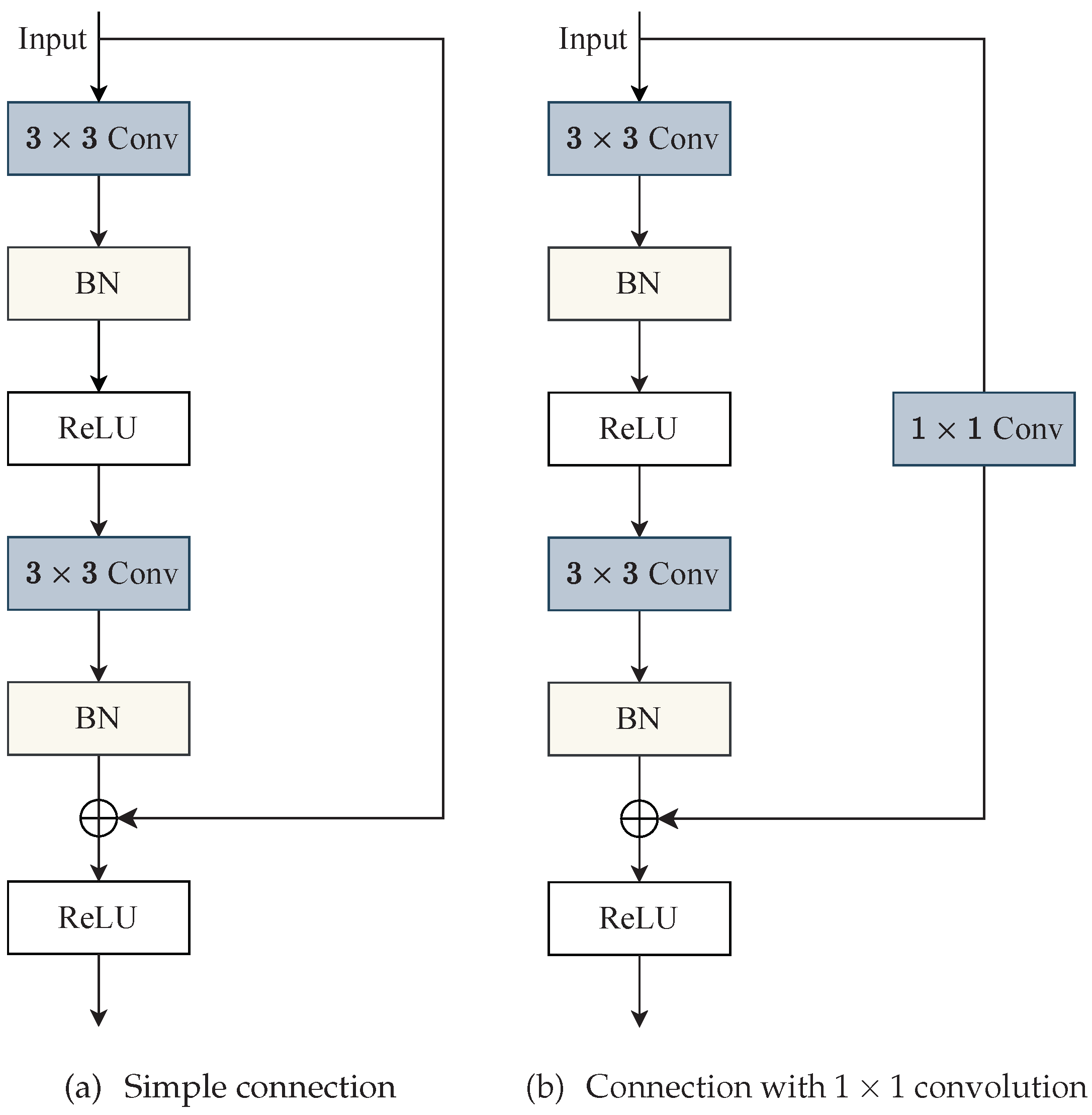
In ResNet18, a basic block is the simplest building block of the network architecture. It consists of two convolutional layers with a residual connection between them. Figure 2 shows that the basic blocks have two different forms depending on the stride used. When the stride is 1, residual connections enable the input to be directly merged with the output of the second convolutional layer by element-wise summation (see Figure 2a). When the stride is not 1, the input is forwarded to a 1 × 1 convolutional layer to achieve dimension increase and downsampling before transferring to the output (see Figure 2b). In practice, all four basic blocks in our ResNet18 have a stride of 2, each of which downsamples the features by half. As a result, aside from the ones produced in the initial phase, the features generated in the successive stages exhibit a decreasing size ratio of 1 / 2 , 1 / 4 , 1 / 8 , and 1 / 16 relative to the original images. The depths of the five stages are 64, 64, 128, 256, and 512 in succession. Except for the output of the last basic block, which is projected into semantic tokens by the tokenizer and further processed by the transformer module, the producing features of the remaining four stages are transmitted to the cascaded decoder to concatenate with high-level features.

3.1.3. Tokenizer and Transformer Module

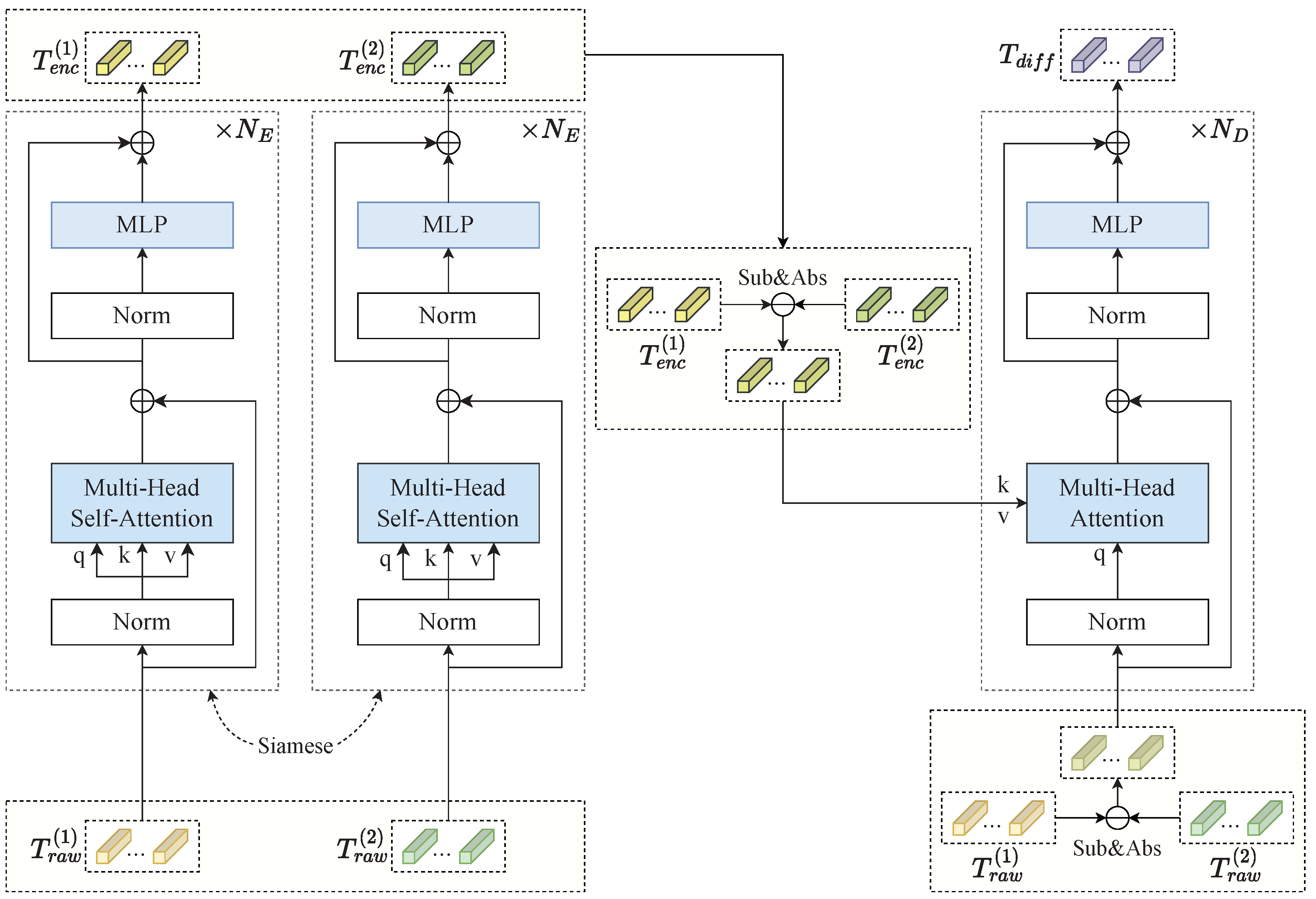
Context modelling is a fundamental aspect for facilitating the network to concentrate on pertinent changes and differentiate between spurious changes such as those attributed to variations in illumination. Therefore, the transformer module, which comprises both transformer encoder and transformer decoder components (see Figure 1a), is incorporated to enable modelling of the spatio-temporal contextual information.
  • Tokenizer:
The highest features of each image extracted by the Siamese backbone are embedded into a set of semantic tokens by the Siamese tokenizer before feeding into the transformer module. Let F ( 1 ) , F ( 2 ) R C × H × W denote the input features, where H × W is the spatial size and C is the channel dimension. For the feature of each temporal, we divide and flatten it into a sequence of patches x p R L × ( P 2 · C ) , where L = H W / P 2 is the length of the patch sequence, and P × P is the spatial size per patch. Afterward, a convolution operation with the filter size of P × P and stride of P projects the patch sequence into the latent embedding space ( C h ), thus obtaining a sequence of tokens. Finally, a trainable positional embedding E p o s R L × C h is incorporated into the token sequence to retain the position information. Formally,
T r a w ( i ) = [ x p 1 E ; x p 2 E ; ; x p L E ] + E p o s , i = 1 , 2
where E R ( P 2 · C ) × C h is the patch embedding that maps patches into latent space. Consequently, the semantic tokens T r a w ( 1 ) , T r a w ( 2 ) R L × C h are produced.
  • Transformer Encoder:
Given the semantic tokens of the raw images, our transformer encoder establishes global semantic relations in token space and captures long-range dependencies among embedded tokens. As shown in Figure 3, we employ N E layers of Siamese encoders, each consisting of a multi-head self-attention (MSA) block and a multi-layer perception (MLP) block, following the standard transformer architecture [26]. Additionally, consistent with ViT [27], layer normalization (LN) is performed before the MSA/MLP, while the residual connection is placed after each block. The input to MSA in layer l is a triple (query Q, key K, value V) computed from the output in the prior layer through three linear projection layers. Formally,
Q = T l 1 e · ( W q ) l j K = T l 1 e · ( W k ) l j V = T l 1 e · ( W v ) l j
where ( W q ) l j , ( W k ) l j , ( W v ) l j R C h × d | j = 1 , , h are the trainable parameter matrices, d is the channel dimension of them, and h is the number of self-attention heads. The self-attention mechanism models global dependencies by computing the weighted average of the values per position. Formally,
A l j ( Q , K , V ) = S o f t m a x ( Q · K T d ) · V
where S o f t m a x ( · ) denotes the Softmax function applied on the channel domain. To capture a wider spectrum of information, the transformer encoder uses MSA to jointly process semantic tokens from different positions. This procedure can be expressed in the subsequent equation:
M S A ( T l 1 e ) = C o n c a t ( A l 1 , , A l h ) · W O
where C o n c a t ( · ) denotes concatenating the outputs of independent self-attention heads, and W O R h d × C h denotes the linear projection matrices.
The MLP architecture comprises two linear layers sandwiching a Gaussian error linear unit (GELU) activation function [67]. Formally,
M L P ( T l 1 e ) = G E L U ( T l 1 e · W 1 ) · W 2
where W 1 R C h × 2 C h , W 2 R 2 C h × C h are learnable linear projection matrices.
To summarize, the computational procedure of the transformer encoder at a specific layer l can be written as:
T 0 e = T r a w ( i ) , i = 1 , 2
( T l e ) = M S A ( L N ( T l 1 e ) ) + T l 1 e , l = 1 , , N E
T l e = M L P ( L N ( ( T l e ) ) ) + ( T l e ) , l = 1 , , N E
The raw embedded tokens T r a w ( 1 ) , T r a w ( 2 ) are converted into context-rich tokens T e n c ( 1 ) , T e n c ( 2 ) R L × C h after N E layers of encoding in the Siamese transformer encoder, respectively. The Siamese transformer encoder effectively captures high-level semantic information about changes of interest.
  • Transformer Decoder:
To capture strongly discriminative semantic information, the transformer decoder projects encoded tokens back into pixel space, resulting in refined feature representations enhanced with spatio-temporal context. In the proposed transformer module (see Figure 3), the embedded tokens T r a w ( 1 ) and T r a w ( 2 ) derived from features F ( 1 ) and F ( 2 ) , respectively, as well as encoded context-rich tokens T e n c ( 1 ) and T e n c ( 2 ) are passed to the transformer decoder to develop correlations between each pixel of differential features and encoded differential tokens. In practice, the raw tokens T r a w ( 1 ) and T r a w ( 2 ) and encoded tokens T e n c ( 1 ) and T e n c ( 2 ) are performing absolute differences separately and input into the transformer decoder to directly generate pixel-level highly discriminative differential features.
The transformer decoder comprises N D layers of decoders. The transformer encoder and decoder share the same architecture except for the fact that the decoder uses multi-head attention (MA) blocks, while the encoder uses multi-head self-attention (MSA) blocks. Here, T r a w ( 1 ) and T r a w ( 2 ) denote queries and T e n c ( 1 ) and T e n c ( 2 ) provide keys. At each layer l, the output T l 1 d of the prior layer and encoded differential tokens serve as the input, and the decoder performs the following computations:
T 0 d = ( | T r a w ( 1 ) T r a w ( 2 ) | , | T e n c ( 1 ) T e n c ( 2 ) | )
( T l d ) = M A ( L N ( T l 1 d ) , | T e n c ( 1 ) T e n c ( 2 ) | ) + T l 1 d , l = 1 , , N D
T l d = M L P ( L N ( ( T l d ) ) ) + ( T l d ) , l = 1 , , N D
T d i f f = L N ( T N D d )
Finally, the decoded refined semantic tokens T d i f f R L × C h are unfolded and reshaped into 3D features F d i f f R C h × H × W .

3.1.4. Cascaded Decoder

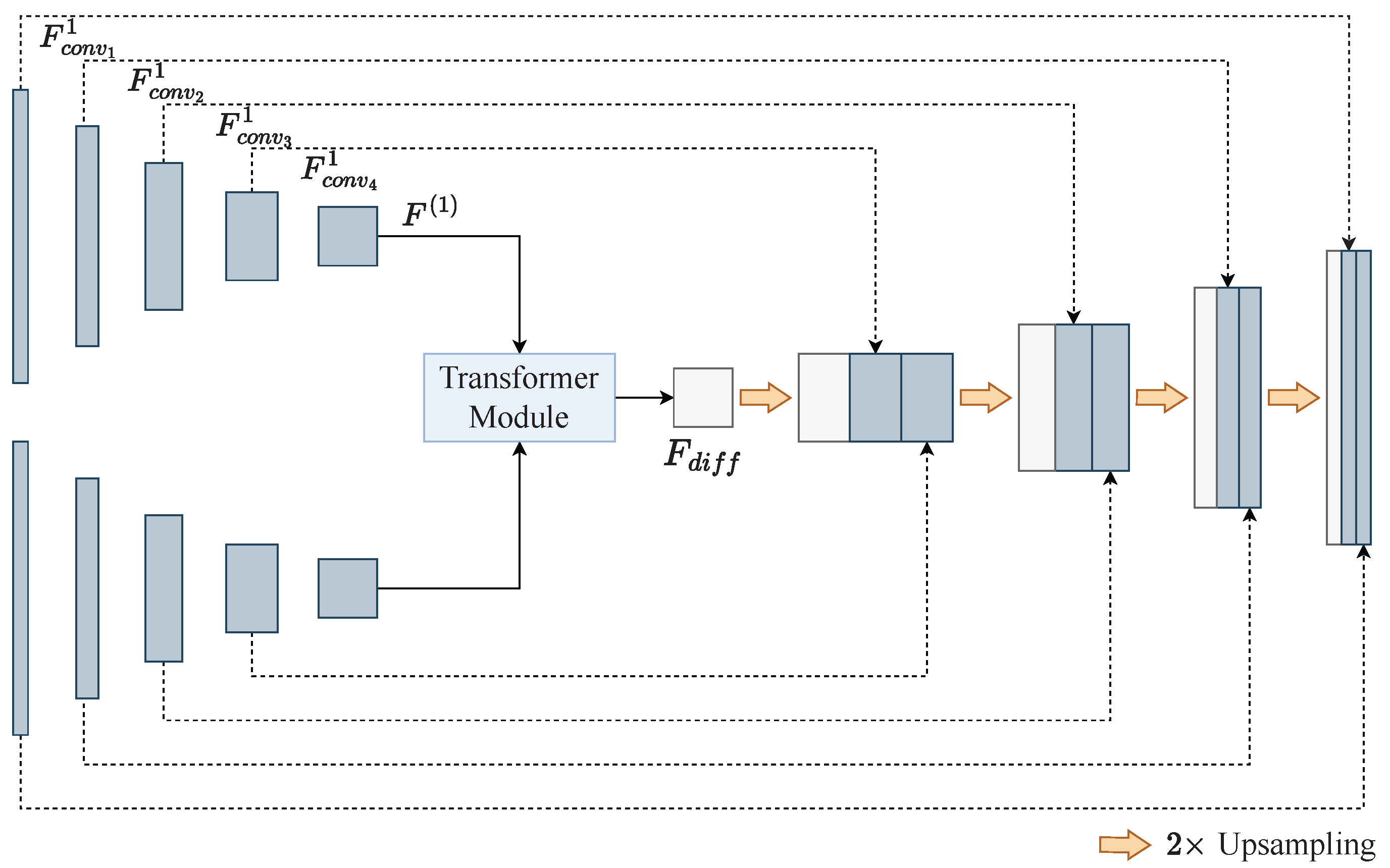
There are different levels of information contained within varying layers of features extracted from raw images. Deep features are highly abstract but lack local information, whereas shallow features contain richer local details but are not as abstract. For the comprehensive learning of both deep and shallow representations, we propose a cascaded decoder, which incorporates highly abstract deep features with shallow features encompassing abundant local information through skip connections, thus alleviating the degradation of details induced by global upsampling and localizing objects with greater precision.
The cascaded decoder consists of four upsampling blocks arranged in a series, as illustrated in Figure 1b. In each upsampling block, the differential features are upscaled and concatenated with the features extracted by the Siamese backbone to learn multilevel representations. A more intuitive description is shown in Figure 4.
Each upsampling block sequentially performs 2 × upsampling, concatenation, and convolution operations on the input. In practice, the differential features reconstructed by the transformer module are first upsampled to the same scale as the penultimate layer features exacted by the Siamese backbone. Then, the upsampled output is concatenated with the corresponding features of individual raw images. Finally, concatenated features successively go through two convolutional layers, BN layers and ReLU layers, yielding the results of the first upsampling block. The remaining upsampling blocks process similarly, as shown in Figure 5.
The following formulation can be used to express the computation carried out in the upsampling block.
F c a t = C o n c a t ( U p S a m p ( i n p u t ) , f e a t u r e 1 , f e a t u r e 2 )
F u p = R e L U ( B N ( f 3 × 3 ( F c a t ) ) )
F u p = R e L U ( B N ( f 3 × 3 ( F u p ) ) )
where U p S a m p ( · ) denotes 2 × upsampling operation on the input, and C o n c a t ( · ) refers to the concatenation of the upsampled input, feature1, and feature2 in the channel dimension.

3.1.5. CBAM

Skip connections fuse the highly abstract differential features with the lower-level features from individual raw images. However, due to the semantic gaps between heterogeneous features, direct feature concatenation cannot achieve good training results. Thus, we introduce CBAM to the cascaded decoder to efficiently combine multilevel features. Since the semantic gap between the fused features in the last upsampling block is the largest, we add CBAM to this block to promote fusion, as shown in Figure 1b.
CBAM is a lightweight module with low memory requirements and computational costs. CBAM consists of two sub-modules, channel attention module (CAM) and spatial attention module (SAM), which help to emphasize the change-related information across different domains. Specifically, during the final upsampling block, the operation within the dashed box in Figure 5 undergoes CAM and SAM procedures at its front-end and back-end, respectively. The role of CAM is to emphasize channels that are pertinent to changes while inhibiting the ones that are not relevant. The function of SAM is to magnify the distances among altered and unaltered pixels across the spatial dimension. In this way, the interested changed areas in the change map are better identified.
We refer to the concatenated features in the fourth upsampling block as F c a t 4 . As shown in Figure 1c, F c a t 4 are forwarded into the max pooling layer and average pooling layer to extract vectors with dimension C c a t 4 × 1 × 1 , where C c a t 4 is the number of channels. Each vector then enters the weight-shared MLP, and the outputs are merged into a single vector by element-wise summation. Notably, the MLP in CBAM consists of two linear layers with a ReLU non-linear activation in between, which is different from the MLP in the transformer. Eventually, the Sigmoid function allocates attention weights to each channel, yielding the channel attention map denoted as M C . Formally,
M C = σ ( M L P ( M a x p o o l ( F c a t 4 ) ) + M L P ( A v g p o o l ( F c a t 4 ) ) )
where σ ( · ) symbolizes the Sigmoid function, and M a x p o o l ( · ) and A v g p o o l ( · ) denote max pooling and average pooling operations, respectively. The channel-wise refined feature F C is obtained by multiplying F c a t 4 with the elements of the channel attention map M C . Formally,
F C = F c a t 4 M C
where ⊗ means element-wise multiplication.
After the channel-wise refinement, F C is performs a convolution operation consistent with the previous three upsampling blocks, and the resulting feature is denoted as F u p 4 . F u p 4 is further refined through SAM on the spatial domain. Specifically, the input feature passes through two pooling layers to generate matrices with dimension 1 × H 0 × W 0 . Then, the concatenated matrices undergo a convolutional layer and a Sigmoid function to output the spatial attention map M S (see Figure 1d). Formally,
M S = σ ( f 7 × 7 ( [ M a x p o o l ( F u p 4 ) ; A v g p o o l ( F u p 4 ) ] ) )
where [ ; ] means concatenation and f 7 × 7 ( · ) means a convolution operation with a filter size of 7 × 7 . Eventually, feature F u p 4 is improved in the spatial dimension through element-wise multiplication with M S , producing the spatial-wise refined feature F S . Formally,
F S = F u p 4 M S
Overall, feature F c a t 4 is further enhanced across the channel and spatial domains during the last upsampling block to facilitate difference discrimination.
Until here, we have obtained discriminative features F S with the spatial size of H 0 × W 0 , consistent with the size of raw images. The classifier comprised of a convolutional layer and a Softmax function is applied to F S to generate a two-channel predicted change probability map P R 2 × H 0 × W 0 . The process of producing a binary change map involves performing an Argmax operation on P in the channel dimension on a pixel-by-pixel basis.

3.2. Datasets

We conduct experiments using two publicly available high-resolution remote sensing change detection datasets, namely LEVIR-CD [2] and SYSU-CD [16].
The LEVIR-CD dataset contains 637 pairs of Google Earth images of size 1024 × 1024 pixels with a spatial resolution of 0.5 m/pixel. Image pairs spanning 5 to 14 years were gathered from 2002 to 2018 at various sites in different cities in Texas. The introduction of variations in seasons and lighting conditions within the dataset helps to examine whether the model can mitigate the interference of pseudo changes. The dataset focuses on changes related to buildings, including both the addition and reduction in buildings. In accordance with the partitioning approach utilized by the developers of the LEVIR-CD dataset, the dataset is segmented into three subsets, namely 70% of the data reserved for training, 10% allocated for validation, and the remaining 20% designated for testing purposes. To accommodate the GPU memory limitations, every image is cut into non-overlapping sub-images measuring 256 × 256 pixels. Consequently, the dataset is comprised of 7120/1024/2048 pairs of sub-images with the purpose of training/validation/testing, respectively.
The SYSU-CD dataset consists of 20,000 pairs of aerial images captured in Hong Kong between 2007 and 2014. Every image is 256 × 256 pixels in size and has a spatial resolution of 0.5 m/pixel. Unlike the LEVIR-CD dataset, there are multiple change types in the SYSU-CD dataset, including new urban buildings, expansion into suburban areas, groundwork before construction, changes in vegetation, expansion of roads, and offshore construction. Notably, the SYSU-CD dataset poses a significant challenge for change detection due to the intricate nature of its scenes and varied types of changes. We adopt the original division approach made by reference [16], which yields 12,000/4000/4000 pairs of images for training/validation/testing, respectively.

4. Experiments and Analysis

4.1. Training Details

The implementation of our model utilizes PyTorch and underwent training on a singular NVIDIA RTX A5000 GPU, which possesses a memory capacity of 24 G. We perform regular data augmentation, including flipping, rescaling, cropping, and Gaussian blurring on the input images. During the training phase, the optimization of network parameters is achieved through the minimization of the cross-entropy loss function. Furthermore, we utilize stochastic gradient descent (SGD) as the model optimizer with a momentum of 0.9 and a weight decay of 0.0005. The initial learning rate is 0.01 and decays linearly with the increase of epochs until it reaches 0. The batch size is defined as 8. The number of epochs is specified as 200. The transformer encoder is configured with a single layer ( N E = 1 ), while the transformer decoder has eight layers ( N D = 8 ). The length of the semantic tokens is 256 ( L = 256 ) and C h is 128. The model undergoes evaluation on the validation set after every training epoch, and the one with the highest performance is chosen as the ultimate model for assessment on the test set.

4.2. Evaluation Metrics

We utilize the F1-score and intersection-over-union (IoU) associated with the change category as the primary quantitative evaluation metrics. In addition, precision and recall of the change category and overall accuracy (OA) are also recorded. F 1 -score takes both Precision and Recall into account and is calculated as follows:
F 1 = 2 · P r e c i s i o n · R e c a l l P r e c i s i o n + R e c a l l
where Precision and Recall are defined as follows:
P r e c i s i o n = T P T P + F P
R e c a l l = T P T P + F N
The IoU is defined as:
I o U = T P T P + F N + F P
The OA is defined as:
O A = T P + T N T P + T N + F N + F P
where TP, FP, and FN denote the number of true positives, false positives, and false negatives, respectively.

4.3. Performance Comparison

The complexity of a machine learning model is typically measured by its number of model parameters (Params) and floating-point operations per second (FLOPs). Specifically, our model exhibits the Params of 15.94 M and FLOPs of 35.02 G, which serve as informative references in this regard.
Within this section, we demonstrate the superiority of our presented model by comparing it with several recent deep learning-based techniques, which are:
  • Fully Convolutional Early Fusion (FC-EF) [18]: The approach involves concatenating bi-temporal images along the channel dimension and passing them as a single input into a fully convolutional network (FCN) for change detection.
  • Fully Convolutional Siamese-Concatenation (FC-Siam-Conc) [18]: The approach utilizes Siamese FCN to extract multilevel features from input images. Feature concatenation is performed in the channel dimension to make change decisions.
  • Fully Convolutional Siamese-Difference (FC-Siam-Diff) [18]: This approach utilizes the Siamese FCN to extract multilevel features from bi-temporal images and subsequently applies feature differencing to determine changes.
  • Spatial–Temporal Attention Neural Network (STANet) [2]: This approach employs self-attention mechanisms to model spatial–temporal relations and obtain more discriminative features. The ultimate change map is produced by metric learning.
  • Dual Task Constrained Deep Siamese Convolutional Network (DTCDSCN) [12]: This method incorporates a dual attention module (DAM) in the Siamese FCN to explore more discriminative representations for change detection.
  • Image Fusion Network (IFNet) [13]: This is a deeply supervised multi-scale feature fusion network, which is composed of a deep feature extraction network with shared weights and a difference discrimination network.
  • Bitemporal Image Transformer (BIT) [8]: This method utilizes spatial attention to condense the feature maps of each temporal into a collection of tokens. Transformer is used to model context in token space to obtain refined features.
  • ChangeFormer [28]: This is a purely transformer-based network, where Siamese transformers are used to extract features of bi-temporal images, and the obtained multi-scale features are differenced and then aggregated in the MLP decoder for change detection.
These methods mentioned above include three purely CNN-based methods (FC-EF, FC-Siam-Conc, and FC-Siam-Diff), three attention-based methods (STANet, DTCDSCN, and IFNet), and two transformer-based methods (BIT and ChangeFormer).

4.3.1. Comparison on the LEVIR-CD Dataset

We compare the proposed model with eight different deep learning-based methods mentioned above on the LEVIR-CD dataset. Since the dataset used in the experiments is divided in the same way, the comparison results are mainly based on reference [28], as shown in Table 1. It is evident that our proposed method has delivered exceptional results in F1, IoU, and OA metrics, scoring 91.21, 83.85, and 99.11%, respectively. The three purely CNN-based methods perform the worst. Among them, FC-Siam-Diff shows relatively good results, with 4.90 and 7.93% lower F1 and IoU scores, respectively, compared to CTCANet. The three attention-based methods have improved effect but still fall short of the transformer-based methods. ChangeFormer achieves 90.40 and 82.48% in F1 and IoU, respectively, achieving suboptimal results. CTCANet outperforms ChangeFormer in all metrics, with F1 and IoU increasing by 0.81 and 1.37%, respectively, making it the best performing method on the LEVIR-CD dataset.
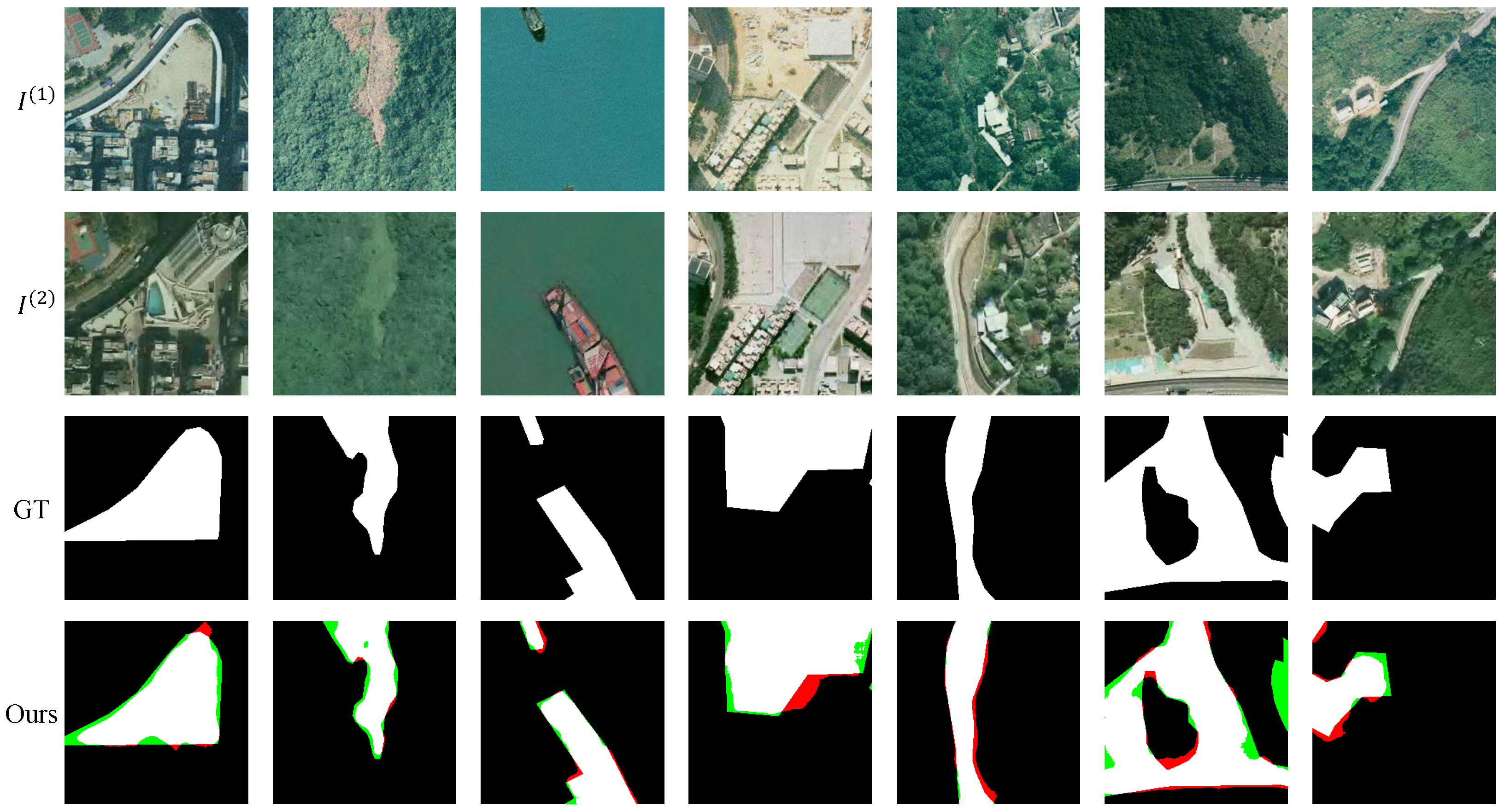
Figure 6 illustrates the change detection outcomes of CTCANet on the LEVIR-CD test set, with the first three rows depicting the bi-temporal images ( I ( 1 ) , I ( 2 ) ) and the corresponding ground truth (GT). The last row is the detection results of our proposed model, where different colours denote different meanings. The white part denotes TP, indicating that the real changes have been detected. The red part denotes FP, which indicates that the regions unchanged are misidentified as actual changes. The green part denotes FN, which means the real changes that are not observed. Despite the significant changes in illumination present in the raw images of the first two columns, the detection results of CTCANet closely resemble the real labels. In addition to changes in lighting conditions, the two images in the third column were taken during different seasons, and the growth patterns of the grass plants are also altered. Nevertheless, our model satisfactorily predicts the change map even for a very small changed area. In the fourth, fifth, and sixth columns, vegetation and road changes are irrelevant changes affecting building change detection. CTCANet can accurately identify changes in large buildings, ensuring regular boundaries and internal structural integrity. These observations suggest that our model is effective in distinguishing between actual and pseudo changes. Despite the intricate scene and abundant irrelevant changes contained in the final column, our model can still provide a reasonable prediction of the location and boundary of the real changes, with few identification errors and missed detections.
Meanwhile, reference [28] provided access to their source code and predicted test image results to conduct comparative analysis. We evaluate our superiority by comparing the test images, as shown in Figure 7. In addition to real changes in buildings, the original image pair contains irrelevant changes, such as road changes, which interfere with change detection. The visualization outcomes demonstrate that our proposed method is more effective in preventing FP and FN compared to other methods, as evidenced by the lower percentage of red and green colours. This indicates that the transformer module we introduced has a promising impact. The changes identified by the other models are somewhat inaccurate. The green region in the ChangeFormer predicted map is the missed detection that resulted from not employing convolution for feature extraction, reflecting the necessity of combining convolution with the transformer.

4.3.2. Comparison on the SYSU-CD Dataset

Unlike the compared methods used in the LEVIR-CD dataset, the predicted results of DTCDSCN, IFNet, and ChangeFormer on the SYSU-CD dataset are not found. We choose another two methods to replace them, which are:
  • Deeply Supervised Attention Metric-Based Network (DSAMNet) [16]: This is a deeply supervised attention-based method, incorporating CBAM to provide more discriminative features for metric learning, and deep supervision to improve the feature extraction ability of hidden layers.
  • Hybrid-TransCD [29]: This is a hybrid multi-scale transformer-based framework that effectively captures image features at multiple levels of granularity by employing detailed self-attention mechanisms.
Table 2 presents a quantitative evaluation of various methods on the SYSU-CD dataset. These comparison results are primarily based on reference [29]. Compared with all the other methods, CTCANet achieves the highest scores in F1, IoU, and OA, which are 81.23 and 68.40, and 91.40%, respectively. The method with the highest precision is FC-Siam-Diff, but its recall is the lowest among all methods, which is 20.77% worse than our proposed model, resulting in the FC-Siam-Diff with the lowest F1. Contrary to the results on the LEVIR-CD dataset, FC-Siam-Diff is the least effective of the three purely CNN-based methods. The reason for the poor results obtained by FC-Siam-Diff can be attributed to two factors. Firstly, the dataset contains multiple change types and complex scenes, which pose a challenge to the model to accurately detect changes. Secondly, the application of difference fusion in FC-Siam-Diff results in the filtration of useful information from the extracted features, further exacerbating the prediction performance. The two attention-based methods achieve relatively good results, with DSAMNet even slightly better than the transformer-based method BIT. Hybrid-TransCD is the second highest scoring model due to the hybrid transformer structure with 80.13 and 66.84% on F1 and IoU, respectively. Our proposed model enhances F1 and IoU by 1.10 and 1.56%, respectively, over Hybrid-TransCD.
Similarly, the outcomes of CTCANet on SYSU-CD test set are graphically illustrated in Figure 8. Since the SYSU-CD dataset contains multiple change types, we list the visual results corresponding to each type below. The first column shows the change detection of new urban buildings. Our model adeptly discerns the changed region within the intricate scene, exhibiting a strong agreement with the ground truth. The second column reflects vegetation changes, and CTCANet identifies vegetation growth effectively. The third column displays the detection of ship changes. The proposed model accurately detects changes in both an increase and a reduction in the number of ships. The groundwork before construction is shown in the fourth column. Despite the comparatively small change between the images, our model locates the modified area. Moreover, CTCANet correctly detects road expansion with complete boundaries, as shown in the fifth column. The raw images in the last two columns contain not only changes in vegetation but also changes in buildings and roads. Hearteningly, CTCANet maintains the boundary information and internal integrity within the changed regions despite a small number of omissions.

5. Discussion

5.1. Discussion of the Fusion Strategy

To explore the most appropriate way to fuse bi-temporal semantic tokens in the transformer module, we design three strategies, which are:
Early-concatenation: As shown in Figure 9, the bi-temporal semantic tokens are first concatenated and provided as input to the transformer encoder to facilitate global modelling. Subsequently, the encoded tokens are split and fed to the Siamese transformer decoder, which generates enriched tokens containing contextual information for each temporal. The projection of these decoded tokens back to the pixel space results in the generation of refined features, which exhibit enhanced concept representation compared to the original ones. Finally, the differential feature maps that are further passed into the cascaded decoder are obtained by performing absolute differences on the two refined features. Since the concatenation takes place at the front of the transformer module, we call the fusion strategy early-concatenation.
Middle-difference: As shown in Figure 10, the bi-temporal semantic tokens are first input into the Siamese transformer encoder to establish global relations. The encoded differential tokens are then forwarded into the transformer decoder together with the original differential tokens, and the change relations between them are explored to directly obtain the refined differential tokens. Finally, the differential tokes are converted back into pixel space, resulting in the creation of discriminative feature maps. As the difference fusion operation is in the interior of the transformer module, we call it middle-difference.
Late-difference: As shown in Figure 11, the Siamese transformer module takes in bi-temporal semantic tokens, which consist of both past and present temporal information, and uses its Siamese encoder and decoder components to capture extensive relationships between the tokens, producing highly contextualized semantic tokens as output. The two sets of context-rich tokens are then projected separately to pixel space, producing refined feature maps. Bi-temporal information is fused by absolute difference operation on the two feature maps. Since the fusion operation appears at the end of the transformer module, we call it late-difference.
Table 3 displays the quantitative outcomes of the three fusion strategies on the two datasets. The hyper-parameters used in the experiments are the same. Here, we only compare the two main evaluation metrics, F1 and IoU. The three fusion strategies perform similarly on the LEVIR-CD dataset, with middle-difference having a slight advantage. For the SYSU-CD dataset, middle difference is 1.88 and 2% higher than early-concatenation and late-difference on F1, and 2.63 and 2.80% higher on IoU, respectively, which proves the leading role of the middle-difference strategy. Meanwhile, we plot the qualitative results of the three strategies on the SYSU-CD dataset in Figure 12. In agreement with the quantitative outcomes, middle-difference has optimal performance, while the early-concatenation and late-difference approaches tend to have higher rates of both false positives and false negatives. This is reflected in the proportion of red and green parts, which are higher for the latter two methods. Therefore, we adopt middle-difference as the bi-temporal information fusion strategy of our proposed model.

5.2. Effect of the Proposed Modules

The proposed CTCANet integrates the transformer module, cascaded decoder, and CBAM to improve the accuracy of change detection. To assess the contribution of each module to the overall network structure, the following ablation experiments are designed:
  • Base: Only the Siamese backbone is employed. The deepest features of the two branches are upsampled to the original size after computing the absolute differences between them. The change map is obtained by the classifier.
  • Proposal1: Compared with the "Base" method, the transformer module is combined to verify its effect on change detection. Notably, middle-difference is adopted in the transformer module for information interaction of bi-temporal tokens.
  • Proposal2: Compared with the “Base” method, the cascaded decoder is used instead of global upsampling to gradually recover the image information, so as to verify the role of the cascaded decoder in the network.
  • Proposal3: In addition to the Siamese backbone, both the transformer module and cascaded decoder are employed.
  • Proposal4: Compared with CTCANet, CBAM is added to each upsampling block of the cascaded decoder instead of only the last one, so as to verify the impact of the CBAM incorporation method on the detection.
Table 4 displays the quantitative outcomes on two datasets. It indicates that the performance of CTCANet is improved through the integration of the transformer module, cascaded decoder, and CBAM, achieving the most favourable results on both datasets. After adding the transformer module, the “Proposal1” method increases the F1 and IoU by 0.71 and 1.17% on LEVIR-CD and by 0.34 and 0.48% on SYSU-CD, compared to the “Base” method, respectively. It shows that the transformer module possessing the capability to capture long-range dependencies does enhance the power of the model. Furthermore, the “Proposal2” method achieves improvements of 0.74 and 1.22% in F1 and IoU on LEVIR-CD, and 1.29 and 1.80% on SYSU-CD, respectively. These results suggest that the cascaded decoder contributes significantly to increasing the effectiveness of the model. Furthermore, the “Proposal3” method, which combines the transformer module and cascaded decoder, outperforms the “Base” method. Specifically, the F1 and IoU of the “Proposal3” method on LEVIR-CD improve by 0.98 and 1.62%, respectively, while the corresponding improvements on SYSU-CD are 1.47 and 2.06%. The superior performance of the “Proposal3” method not only demonstrates the effect and robustness of the transformer module and cascaded decoder, but also the gaining effectiveness of their incorporation.
The results of adding CBAM to each upsampling block of the cascaded decoder are not ideal. Compared to the model without CBAM, the “Proposal4” method increases F1 and IoU on the LEVIR-CD dataset by 0.13 and 0.22%, respectively, with a small effect improvement; nevertheless, those on the SYSU-CD dataset decline by 0.57 and 0.81%, respectively. This can be attributed to the fact that the SYSU-CD dataset contains complex scenes and multiple types of changes, making it more challenging for the model to accurately identify changes. These findings suggest that while CBAM may enhance the model to detect changes in simpler scenes, it may not always be effective in more complex scenarios. Integrating CBAM in each upsampling block does not smooth the semantic gaps, but increases the training difficulty, leading to poor model performance. Therefore, the CBAM is selectively used in the last upsampling block of the cascaded decoder, where the semantic gaps are large, and one CBAM does not increase the training load of the model. Eventually, CTCANet outperforms the “Proposal3” method (the method without CBAM) in terms of F1 and IoU by 0.39 and 0.67% on the LEVIR-CD dataset, by 0.13 and 0.19% on the SYSU-CD dataset, respectively.
We further corroborate the role of each module by comparing visual results on the two datasets. As shown in Figure 13, the first three rows are the predicted results from the LEVIR-CD dataset, and the last three are from the SYSU-CD dataset. The comparison between columns (d) and (e) reveals that the inclusion of the transformer module is helpful to reduce pseudo changes and detect large-area changed regions, ascribed to the reality that the transformer is not limited by the receptive field and can globally model spatio-temporal context. In addition, the comparison of columns (d) and (f) in the second and third rows proves the impact of the cascaded decoder. Visualization outcomes show that integrating the cascaded decoder can lead to more complete boundaries and higher internal compactness while enhancing the detection of small change targets. The results in column (g) show that the model integrating the transformer and cascaded decoder performs better than the model integrating only one of the modules. The results of the last three columns demonstrate the effect of CBAM. Compared with column (g), the red area in column (i) is reduced, that is, there are fewer false detections, which proves that CBAM plays a positive role in increasing attention to real changes and suppressing irrelevant changes. On the other hand, the comparison of columns (i) and (h) indicates that the incorporation method of CBAM has a significant influence on the detection. Most importantly, CTCANet, which combines the transformer module, cascaded decoder, and CBAM, considerably improves the completeness and accuracy of detection results (with the least missed and false alarms), further proving the effectiveness of our modules.
Besides conducting a comparative analysis of the quantitative and qualitative outcomes, we additionally present a graphical representation of the accuracy curves for the “Base” and CTCANet models on the LEVIR dataset concerning training stages (see Figure 14). These curves capture the mean F1-score of the training and validation sets across a span of 200 epochs. Our examination of the results reveals that while the two methods exhibit comparable performance on the training set, CTCANet displays higher accuracy values and greater stability on the validation set. These findings provide compelling evidence for the efficacy of the proposed modules in enhancing model performance and augmenting generalization.

5.3. Discussion of Backbone

Our model uses the modified ResNet18 as the backbone to extract features from images. In order to analyse the effect of the backbone on detection, we delete the last one or two basic blocks of ResNet18 for comparative analysis. We name the backbone with the last one/two basic blocks removed as “Base_S4”/“Base_S3”. All hyper-parameter settings are the same as the "Base" method. On the other hand, we select VGG16 [68] as the backbone to verify the effect of our proposed modules on different backbone networks. The VGG16 structure used in our experiments is the layers before pool5 that have been pre-trained on ImageNet [69]. Table 5 shows the results of the experiments.
The data presented in Table 5 suggests that ResNet18 outperforms VGG16 as the backbone network on both LEVIR-CD and SYSU-CD datasets. When solely the Siamese backbone is employed, ResNet18 exhibits superior performance relative to VGG16, with the LEVIR-CD dataset demonstrating a particular sensitivity to this effect. The robustness of ResNet18 is evident, as removing a single basic block only marginally impacts accuracy outcomes for both datasets. In contrast, removing two basic blocks leads to a reduction in F1 and IoU by 1.57 and 2.55% on LEVIR-CD, and 2.36 and 3.19% on SYSU-CD, respectively. These results indicate that the number of convolutional layers significantly affects the performance of ResNet18. The "CTCANet (VGG16)" model, which employs VGG16 as the backbone, exhibits substantial enhancements in F1 and IoU on both datasets compared to the “Base_VGG16” method, which only utilizes the Siamese backbone. Specifically, the “CTCANet (VGG16)” method yields improvements of 6.69 and 10.39% in F1 and IoU on LEVIR-CD, and 2.29% and 3.03% on SYSU-CD, respectively. These findings suggest that the proposed modules are effective and have different degrees of favourable impact across different backbones.

5.4. Discussion of the Number of Transformer Layers

The number of encoder and decoder layers in the transformer module is the important hyper-parameter. Here, we conduct a series of experiments to explore the optimal configuration. Our findings, presented in Table 6, demonstrate that increasing the number of decoder layers leads to a gradual improvement in model performance across the two datasets. However, when only the number of encoder layers is increased while keeping the number of decoder layers constant, the performance of the model does not show an upward trend. This suggests that the transformer encoder plays an auxiliary role in guiding the decoder to generate semantic features with strongly discriminative information. Ultimately, our analysis indicates that the most favourable arrangement for our model entails the implementation of a solitary encoder layer in conjunction with eight decoder layers.

6. Conclusions

This article proposes a novel CNN-transformer network for high-resolution remote sensing image change detection. Initially, the proposed model utilizes the Siamese backbone to extract hierarchical features from input images. Following this, our tokenizer converts the deepest features of the two branches into semantic tokens, which are subsequently propagated into the transformer module to enable global spatio-temporal context modelling. Here, we design experiments to explore the most appropriate bi-temporal information fusion strategy. After reshaping the context-rich semantic tokens into pixel-level features, the refined high-level features are incorporated with the low-level features from individual raw images using skip connections to reduce the loss of details and better locate the changed regions. At the same time, CBAM is integrated into the last upsampling block of the cascaded decoder to smooth semantic gaps between heterogeneous features. Furthermore, it promotes change detection by highlighting the change of interest and suppressing irrelevant information across the channel and spatial domains. The effectiveness of CTCANet is confirmed by comparing it with some advanced approaches on two open accessible datasets, LEVIR-CD and SYSU-CD. The findings suggest that the presented approach holds greater potential compared to other methods.

Author Contributions

Conceptualization, M.Y., Z.C. and C.Z.; methodology, M.Y.; software, M.Y.; validation, M.Y.; writing—original draft preparation, M.Y.; writing—review and editing, M.Y., Z.C. and C.Z.; visualization, M.Y.; supervision, M.Y., Z.C. and C.Z.; project administration, Z.C.; funding acquisition, Z.C. All authors have read and agreed to the published version of the manuscript.

Funding

This research was funded by the National Forestry and Grassland Administration of China, grant number 2021133108. The funding program is known as “Forestry, Grass Technology Promotion APP Information Service”.

Data Availability Statement

Not applicable.

Conflicts of Interest

The authors declare no conflict of interest.

Abbreviations

The following abbreviations are used in this manuscript:
CNNConvolutional Neural Networks
CBAMConvolutional Block Attention Module
GANGenerative Adversarial Network
RNNRecurrent Neural Network
NLPNatural Language Processing
ViTVision Transformer
MLPMulti-Layer Perception
PVTPyramid Vision Transformer
CAMChannel Attention Module
SAMSpatial Attention Module
BNBatch Normalization
ReLURectified Linear Unit
MSAMulti-Head Self-Attention
GELUGaussian Error Linear Unit
MAMulti-Head Attention
SGDStochastic Gradient Descent
IoUIntersection-Over-Union
OAOverall Accuracy
GTGround Truth
ParamsParameters
FLOPsFloating-Point Operations Per Second
FCNFully Convolutional Network
FC-EFFully Convolutional Early Fusion
FC-Siam-ConcFully Convolutional Siamese-Concatenation
FC-Siam-DiffFully Convolutional Siamese-Difference
STANetSpatial–Temporal Attention Neural Network
DTCDSCNDual Task Constrained Deep Siamese Convolutional Network
IFNetImage Fusion Network
BITBitemporal Image Transformer
DSAMNetDeeply Supervised Attention Metric-Based Network

References

  1. Singh, A. Review article digital change detection techniques using remotely-sensed data. Int. J. Remote Sens. 1989, 10, 989–1003. [Google Scholar] [CrossRef]
  2. Chen, H.; Shi, Z. A spatial-temporal attention-based method and a new dataset for remote sensing image change detection. Remote Sens. 2020, 12, 1662. [Google Scholar] [CrossRef]
  3. Xu, J.Z.; Lu, W.; Li, Z.; Khaitan, P.; Zaytseva, V. Building damage detection in satellite imagery using convolutional neural networks. arXiv 2019, arXiv:1910.06444. [Google Scholar]
  4. Mahdavi, S.; Salehi, B.; Huang, W.; Amani, M.; Brisco, B. A PolSAR change detection index based on neighborhood information for flood mapping. Remote Sens. 2019, 11, 1854. [Google Scholar] [CrossRef]
  5. Zheng, Z.; Zhong, Y.; Wang, J.; Ma, A.; Zhang, L. Building damage assessment for rapid disaster response with a deep object-based semantic change detection framework: From natural disasters to human-made disasters. Remote Sens. Environ. 2021, 265, 112636. [Google Scholar] [CrossRef]
  6. Jin, S.; Yang, L.; Danielson, P.; Homer, C.; Fry, J.; Xian, G. A comprehensive change detection method for updating the National Land Cover Database to circa 2011. Remote Sens. Environ. 2013, 132, 159–175. [Google Scholar] [CrossRef]
  7. Shi, W.; Zhang, M.; Zhang, R.; Chen, S.; Zhan, Z. Change detection based on artificial intelligence: State-of-the-art and challenges. Remote Sens. 2020, 12, 1688. [Google Scholar] [CrossRef]
  8. Chen, H.; Qi, Z.; Shi, Z. Remote sensing image change detection with transformers. IEEE Trans. Geosci. Remote Sens. 2021, 60, 5607514. [Google Scholar] [CrossRef]
  9. Chen, J.; Yuan, Z.; Peng, J.; Chen, L.; Huang, H.; Zhu, J.; Liu, Y.; Li, H. DASNet: Dual attentive fully convolutional Siamese networks for change detection in high-resolution satellite images. IEEE J. Sel. Top. Appl. Earth Obs. Remote Sens. 2020, 14, 1194–1206. [Google Scholar] [CrossRef]
  10. Zhang, M.; Xu, G.; Chen, K.; Yan, M.; Sun, X. Triplet-based semantic relation learning for aerial remote sensing image change detection. IEEE Geosci. Remote Sens. Lett. 2018, 16, 266–270. [Google Scholar] [CrossRef]
  11. Zhang, M.; Shi, W. A feature difference convolutional neural network-based change detection method. IEEE Trans. Geosci. Remote Sens. 2020, 58, 7232–7246. [Google Scholar] [CrossRef]
  12. Liu, Y.; Pang, C.; Zhan, Z.; Zhang, X.; Yang, X. Building change detection for remote sensing images using a dual-task constrained deep siamese convolutional network model. IEEE Geosci. Remote Sens. Lett. 2020, 18, 811–815. [Google Scholar] [CrossRef]
  13. Zhang, C.; Yue, P.; Tapete, D.; Jiang, L.; Shangguan, B.; Huang, L.; Liu, G. A deeply supervised image fusion network for change detection in high resolution bi-temporal remote sensing images. ISPRS J. Photogramm. Remote Sens. 2020, 166, 183–200. [Google Scholar] [CrossRef]
  14. Peng, X.; Zhong, R.; Li, Z.; Li, Q. Optical remote sensing image change detection based on attention mechanism and image difference. IEEE Trans. Geosci. Remote Sens. 2020, 59, 7296–7307. [Google Scholar] [CrossRef]
  15. Jiang, H.; Hu, X.; Li, K.; Zhang, J.; Gong, J.; Zhang, M. PGA-SiamNet: Pyramid feature-based attention-guided Siamese network for remote sensing orthoimagery building change detection. Remote Sens. 2020, 12, 484. [Google Scholar] [CrossRef]
  16. Shi, Q.; Liu, M.; Li, S.; Liu, X.; Wang, F.; Zhang, L. A deeply supervised attention metric-based network and an open aerial image dataset for remote sensing change detection. IEEE Trans. Geosci. Remote Sens. 2021, 60, 5604816. [Google Scholar] [CrossRef]
  17. Ronneberger, O.; Fischer, P.; Brox, T. U-net: Convolutional networks for biomedical image segmentation. In Proceedings of the Medical Image Computing and Computer-Assisted Intervention—MICCAI 2015: 18th International Conference, Munich, Germany, 5–9 October 2015; Springer: Berlin/Heidelberg, Germany, 2015; pp. 234–241. [Google Scholar]
  18. Daudt, R.C.; Le Saux, B.; Boulch, A. Fully convolutional siamese networks for change detection. In Proceedings of the 2018 25th IEEE International Conference on Image Processing (ICIP), Athens, Greece, 7–10 October 2018; IEEE: Piscataway, NJ, USA, 2018; pp. 4063–4067. [Google Scholar]
  19. Peng, D.; Zhang, Y.; Guan, H. End-to-end change detection for high resolution satellite images using improved UNet++. Remote Sens. 2019, 11, 1382. [Google Scholar] [CrossRef]
  20. Fang, S.; Li, K.; Shao, J.; Li, Z. SNUNet-CD: A densely connected Siamese network for change detection of VHR images. IEEE Geosci. Remote Sens. Lett. 2021, 19, 8007805. [Google Scholar] [CrossRef]
  21. Lebedev, M.; Vizilter, Y.V.; Vygolov, O.; Knyaz, V.; Rubis, A.Y. Change detection in remote sensing images using conditional adversarial networks. Int. Arch. Photogramm. Remote Sens. Spat. Inf. Sci. 2018, 42, 565–571. [Google Scholar] [CrossRef]
  22. Hou, B.; Liu, Q.; Wang, H.; Wang, Y. From W-Net to CDGAN: Bitemporal change detection via deep learning techniques. IEEE Trans. Geosci. Remote Sens. 2019, 58, 1790–1802. [Google Scholar] [CrossRef]
  23. Zhao, W.; Mou, L.; Chen, J.; Bo, Y.; Emery, W.J. Incorporating metric learning and adversarial network for seasonal invariant change detection. IEEE Trans. Geosci. Remote Sens. 2019, 58, 2720–2731. [Google Scholar] [CrossRef]
  24. Papadomanolaki, M.; Verma, S.; Vakalopoulou, M.; Gupta, S.; Karantzalos, K. Detecting urban changes with recurrent neural networks from multitemporal Sentinel-2 data. In Proceedings of the IGARSS 2019—2019 IEEE International Geoscience and Remote Sensing Symposium, Yokohama, Japan, 28 July–2 August 2019; IEEE: Piscataway, NJ, USA, 2019; pp. 214–217. [Google Scholar]
  25. Khusni, U.; Dewangkoro, H.I.; Arymurthy, A.M. Urban area change detection with combining CNN and RNN from sentinel-2 multispectral remote sensing data. In Proceedings of the 2020 3rd International Conference on Computer and Informatics Engineering (IC2IE), Yogyakarta, Indonesia, 15–16 September 2020; IEEE: Piscataway, NJ, USA, 2020; pp. 171–175. [Google Scholar]
  26. Vaswani, A.; Shazeer, N.; Parmar, N.; Uszkoreit, J.; Jones, L.; Gomez, A.N.; Kaiser, Ł.; Polosukhin, I. Attention is all you need. Adv. Neural Inf. Process. Syst. 2017, 30. [Google Scholar]
  27. Dosovitskiy, A.; Beyer, L.; Kolesnikov, A.; Weissenborn, D.; Zhai, X.; Unterthiner, T.; Dehghani, M.; Minderer, M.; Heigold, G.; Gelly, S.; et al. An image is worth 16x16 words: Transformers for image recognition at scale. arXiv 2020, arXiv:2010.11929. [Google Scholar]
  28. Bandara, W.G.C.; Patel, V.M. A Transformer-Based Siamese Network for Change Detection. arXiv 2022, arXiv:2201.01293. [Google Scholar]
  29. Ke, Q.; Zhang, P. Hybrid-transcd: A hybrid transformer remote sensing image change detection network via token aggregation. ISPRS Int. J. Geo-Inf. 2022, 11, 263. [Google Scholar] [CrossRef]
  30. Woo, S.; Park, J.; Lee, J.Y.; Kweon, I.S. Cbam: Convolutional block attention module. In Proceedings of the European Conference on Computer Vision (ECCV), Munich, Germany, 8–14 September 2018; pp. 3–19. [Google Scholar]
  31. Nemoto, K.; Hamaguchi, R.; Sato, M.; Fujita, A.; Imaizumi, T.; Hikosaka, S. Building change detection via a combination of CNNs using only RGB aerial imageries. In Remote Sensing Technologies and Applications in Urban Environments II; SPIE: Bellingham, WA, USA, 2017; Volume 10431, pp. 107–118. [Google Scholar]
  32. Ji, S.; Shen, Y.; Lu, M.; Zhang, Y. Building instance change detection from large-scale aerial images using convolutional neural networks and simulated samples. Remote Sens. 2019, 11, 1343. [Google Scholar] [CrossRef]
  33. Liu, R.; Kuffer, M.; Persello, C. The temporal dynamics of slums employing a CNN-based change detection approach. Remote Sens. 2019, 11, 2844. [Google Scholar] [CrossRef]
  34. Daudt, R.C.; Le Saux, B.; Boulch, A.; Gousseau, Y. Urban change detection for multispectral earth observation using convolutional neural networks. In Proceedings of the IGARSS 2018—2018 IEEE International Geoscience and Remote Sensing Symposium, Valencia, Spain, 22–27 July 2018; IEEE: Piscataway, NJ, USA, 2018; pp. 2115–2118. [Google Scholar]
  35. Rahman, F.; Vasu, B.; Van Cor, J.; Kerekes, J.; Savakis, A. Siamese network with multi-level features for patch-based change detection in satellite imagery. In Proceedings of the 2018 IEEE Global Conference on Signal and Information Processing (GlobalSIP), Anaheim, CA, USA, 26–28 November 2018; IEEE: Piscataway, NJ, USA, 2018; pp. 958–962. [Google Scholar]
  36. Wang, M.; Tan, K.; Jia, X.; Wang, X.; Chen, Y. A deep siamese network with hybrid convolutional feature extraction module for change detection based on multi-sensor remote sensing images. Remote Sens. 2020, 12, 205. [Google Scholar] [CrossRef]
  37. De Bem, P.P.; de Carvalho Junior, O.A.; Fontes Guimarães, R.; Trancoso Gomes, R.A. Change detection of deforestation in the Brazilian Amazon using landsat data and convolutional neural networks. Remote Sens. 2020, 12, 901. [Google Scholar] [CrossRef]
  38. Zhao, W.; Chen, X.; Ge, X.; Chen, J. Using adversarial network for multiple change detection in bitemporal remote sensing imagery. IEEE Geosci. Remote Sens. Lett. 2020, 19, 8003605. [Google Scholar] [CrossRef]
  39. Bao, T.; Fu, C.; Fang, T.; Huo, H. PPCNET: A combined patch-level and pixel-level end-to-end deep network for high-resolution remote sensing image change detection. IEEE Geosci. Remote Sens. Lett. 2020, 17, 1797–1801. [Google Scholar] [CrossRef]
  40. Chen, H.; Li, W.; Shi, Z. Adversarial instance augmentation for building change detection in remote sensing images. IEEE Trans. Geosci. Remote Sens. 2021, 60, 5603216. [Google Scholar] [CrossRef]
  41. Fang, B.; Pan, L.; Kou, R. Dual learning-based siamese framework for change detection using bi-temporal VHR optical remote sensing images. Remote Sens. 2019, 11, 1292. [Google Scholar] [CrossRef]
  42. Wang, W.; Xie, E.; Li, X.; Fan, D.P.; Song, K.; Liang, D.; Lu, T.; Luo, P.; Shao, L. Pyramid vision transformer: A versatile backbone for dense prediction without convolutions. In Proceedings of the IEEE/CVF International Conference on Computer Vision, Montreal, BC, Canada, 11–17 October 2021; pp. 568–578. [Google Scholar]
  43. Liu, Z.; Lin, Y.; Cao, Y.; Hu, H.; Wei, Y.; Zhang, Z.; Lin, S.; Guo, B. Swin transformer: Hierarchical vision transformer using shifted windows. In Proceedings of the IEEE/CVF International Conference on Computer Vision, Montreal, BC, Canada, 11–17 October 2021; pp. 10012–10022. [Google Scholar]
  44. Wu, B.; Xu, C.; Dai, X.; Wan, A.; Zhang, P.; Yan, Z.; Tomizuka, M.; Gonzalez, J.; Keutzer, K.; Vajda, P. Visual transformers: Token-based image representation and processing for computer vision. arXiv 2020, arXiv:2006.03677. [Google Scholar]
  45. Chen, C.F.R.; Fan, Q.; Panda, R. Crossvit: Cross-attention multi-scale vision transformer for image classification. In Proceedings of the IEEE/CVF International Conference on Computer Vision, Montreal, BC, Canada, 11–17 October 2021; pp. 357–366. [Google Scholar]
  46. Xie, E.; Wang, W.; Yu, Z.; Anandkumar, A.; Alvarez, J.M.; Luo, P. SegFormer: Simple and efficient design for semantic segmentation with transformers. Adv. Neural Inf. Process. Syst. 2021, 34, 12077–12090. [Google Scholar]
  47. Zheng, S.; Lu, J.; Zhao, H.; Zhu, X.; Luo, Z.; Wang, Y.; Fu, Y.; Feng, J.; Xiang, T.; Torr, P.H.; et al. Rethinking semantic segmentation from a sequence-to-sequence perspective with transformers. In Proceedings of the IEEE/CVF Conference on Computer Vision and Pattern Recognition, Nashville, TN, USA, 20–25 June 2021; pp. 6881–6890. [Google Scholar]
  48. Carion, N.; Massa, F.; Synnaeve, G.; Usunier, N.; Kirillov, A.; Zagoruyko, S. End-to-end object detection with transformers. In Proceedings of the Computer Vision—ECCV 2020: 16th European Conference, Glasgow, UK, 23–28 August 2020; Springer: Berlin/Heidelberg, Germany, 2020; pp. 213–229. [Google Scholar]
  49. Zhu, X.; Su, W.; Lu, L.; Li, B.; Wang, X.; Dai, J. Deformable detr: Deformable transformers for end-to-end object detection. arXiv 2020, arXiv:2010.04159. [Google Scholar]
  50. Yang, F.; Yang, H.; Fu, J.; Lu, H.; Guo, B. Learning texture transformer network for image super-resolution. In Proceedings of the IEEE/CVF Conference on Computer Vision and Pattern Recognition, Seattle, WA, USA, 13–19 June 2020; pp. 5791–5800. [Google Scholar]
  51. Chen, H.; Wang, Y.; Guo, T.; Xu, C.; Deng, Y.; Liu, Z.; Ma, S.; Xu, C.; Xu, C.; Gao, W. Pre-trained image processing transformer. In Proceedings of the IEEE/CVF Conference on Computer Vision and Pattern Recognition, Nashville, TN, USA, 20–25 June 2021; pp. 12299–12310. [Google Scholar]
  52. Chen, M.; Radford, A.; Child, R.; Wu, J.; Jun, H.; Luan, D.; Sutskever, I. Generative pretraining from pixels. In Proceedings of the International Conference on Machine Learning, PMLR, Online, 13–18 July 2020; pp. 1691–1703. [Google Scholar]
  53. Esser, P.; Rombach, R.; Ommer, B. Taming transformers for high-resolution image synthesis. In Proceedings of the IEEE/CVF Conference on Computer Vision and Pattern Recognition, Nashville, TN, USA, 20–25 June 2021; pp. 12873–12883. [Google Scholar]
  54. Li, Z.; Chen, G.; Zhang, T. A CNN-transformer hybrid approach for crop classification using multitemporal multisensor images. IEEE J. Sel. Top. Appl. Earth Obs. Remote Sens. 2020, 13, 847–858. [Google Scholar] [CrossRef]
  55. He, X.; Chen, Y.; Lin, Z. Spatial-spectral transformer for hyperspectral image classification. Remote Sens. 2021, 13, 498. [Google Scholar] [CrossRef]
  56. Deng, P.; Xu, K.; Huang, H. When CNNs meet vision transformer: A joint framework for remote sensing scene classification. IEEE Geosci. Remote Sens. Lett. 2021, 19, 8020305. [Google Scholar] [CrossRef]
  57. Zhang, J.; Zhao, H.; Li, J. TRS: Transformers for remote sensing scene classification. Remote Sens. 2021, 13, 4143. [Google Scholar] [CrossRef]
  58. Xu, X.; Feng, Z.; Cao, C.; Li, M.; Wu, J.; Wu, Z.; Shang, Y.; Ye, S. An improved swin transformer-based model for remote sensing object detection and instance segmentation. Remote Sens. 2021, 13, 4779. [Google Scholar] [CrossRef]
  59. Li, Q.; Chen, Y.; Zeng, Y. Transformer with transfer CNN for remote-sensing-image object detection. Remote Sens. 2022, 14, 984. [Google Scholar] [CrossRef]
  60. Xu, Z.; Zhang, W.; Zhang, T.; Yang, Z.; Li, J. Efficient transformer for remote sensing image segmentation. Remote Sens. 2021, 13, 3585. [Google Scholar] [CrossRef]
  61. Wang, H.; Chen, X.; Zhang, T.; Xu, Z.; Li, J. CCTNet: Coupled CNN and transformer network for crop segmentation of remote sensing images. Remote Sens. 2022, 14, 1956. [Google Scholar] [CrossRef]
  62. Gao, L.; Liu, H.; Yang, M.; Chen, L.; Wan, Y.; Xiao, Z.; Qian, Y. STransFuse: Fusing swin transformer and convolutional neural network for remote sensing image semantic segmentation. IEEE J. Sel. Top. Appl. Earth Obs. Remote Sens. 2021, 14, 10990–11003. [Google Scholar] [CrossRef]
  63. Zhang, C.; Wang, L.; Cheng, S.; Li, Y. SwinSUNet: Pure transformer network for remote sensing image change detection. IEEE Trans. Geosci. Remote Sens. 2022, 60, 5224713. [Google Scholar] [CrossRef]
  64. Wang, G.; Li, B.; Zhang, T.; Zhang, S. A network combining a transformer and a convolutional neural network for remote sensing image change detection. Remote Sens. 2022, 14, 2228. [Google Scholar] [CrossRef]
  65. Wang, W.; Tan, X.; Zhang, P.; Wang, X. A CBAM based multiscale transformer fusion approach for remote sensing image change detection. IEEE J. Sel. Top. Appl. Earth Obs. Remote Sens. 2022, 15, 6817–6825. [Google Scholar] [CrossRef]
  66. He, K.; Zhang, X.; Ren, S.; Sun, J. Deep residual learning for image recognition. In Proceedings of the IEEE Conference on Computer Vision and Pattern Recognition, Las Vegas, NV, USA, 27–30 June 2016; pp. 770–778. [Google Scholar]
  67. Hendrycks, D.; Gimpel, K. Gaussian error linear units (gelus). arXiv 2016, arXiv:1606.08415. [Google Scholar]
  68. Simonyan, K.; Zisserman, A. Very deep convolutional networks for large-scale image recognition. arXiv 2014, arXiv:1409.1556. [Google Scholar]
  69. Krizhevsky, A.; Sutskever, I.; Hinton, G.E. Imagenet classification with deep convolutional neural networks. Commun. ACM 2017, 60, 84–90. [Google Scholar] [CrossRef]
Figure 1. (a) The pipeline of CTCANet. The model mainly includes four parts: Siamese backbone, transformer module, cascaded decoder, and CBAM. (b) Cascaded decoder. The cascaded decoder consists of four upsampling blocks, where the dark grey cuboids represent features extracted by the Siamese backbone. Note that CBAM is added to the last upsampling block. (c) Channel attention module (CAM). (d) Spatial attention module (SAM). CAM and SAM are two sub-modules of CBAM.
Remotesensing 15 02406 g001
Figure 2. Structure of basic blocks from our ResNet18. Employ structure (a) in cases where the stride is equal to 1, and utilize structure (b) in circumstances where the stride is not equivalent to 1.
Remotesensing 15 02406 g002
Figure 3. Illustration of the transformer module. The Siamese transformer encoder takes in raw embedded tokens to model global semantic relations and produce context-rich encoded tokens. The encoded tokens and the raw embedded tokens undergo individual absolute difference operations. Subsequently, the two sets of tokens are forwarded to the transformer decoder, generating tokens with highly discriminative differential information.
Remotesensing 15 02406 g003
Figure 4. Illustration of skip connections. The size-different dark grey rectangles represent scale-varying features extracted by the Siamese backbone. From left to right is F c o n v 1 i , F c o n v 2 i , F c o n v 3 i , F c o n v 4 i , and F ( i ) in turn, where i = 1 , 2 represents two different time phases.
Remotesensing 15 02406 g004
Figure 5. Illustration of the upsampling block. Feature1 and feature2 are the features of I ( 1 ) and I ( 2 ) extracted by the Siamese backbone, respectively.
Remotesensing 15 02406 g005
Figure 6. LEVIR-CD test image results. Red indicates incorrectly identified pixels, while green means missed pixels.
Remotesensing 15 02406 g006
Figure 7. Qualitative results of different change detection methods on LEVIR-CD. Red indicates incorrectly identified pixels, while green means missed pixels.
Remotesensing 15 02406 g007
Figure 8. SYSU-CD test image results. Red indicates incorrectly identified pixels, while green means missed pixels.
Remotesensing 15 02406 g008
Figure 9. Early-concatenation strategy.
Remotesensing 15 02406 g009
Figure 10. Middle-difference strategy.
Remotesensing 15 02406 g010
Figure 11. Late-difference strategy.
Remotesensing 15 02406 g011
Figure 12. Qualitative results of different fusion strategies on the SYSU-CD dataset. Red indicates incorrectly identified pixels, while green means missed pixels. (a) I ( 1 ) . (b) I ( 2 ) . (c) Ground truth. (d) Early-concatenation. (e) Middle-difference. (f) Late-difference.
Remotesensing 15 02406 g012
Figure 13. Visualization results of module ablation experiments. Red indicates incorrectly identified pixels, while green means missed pixels. The first three rows are from the LEVIR-CD dataset and the last three are from the SYSU-CD dataset. (a) I ( 1 ) . (b) I ( 2 ) . (c) Ground truth. (d) Base. (e) Proposal1. (f) Proposal2. (g) Proposal3. (h) Proposal4. (i) CTCANet (Ours).
Remotesensing 15 02406 g013
Figure 14. Visual comparison of learning curves for “Base” methods and CTCANet on LEVIR-CD. (a) Learning curves on the training set. (b) Learning curves on the validation set.
Remotesensing 15 02406 g014
Table 1. Average quantitative results of various change detection methods on LEVIR-CD test set reported as percentages (%), colour-coded with red for highest and blue for second highest values.
MethodsPrecisionRecallF1IoUOA
FC-EF86.9180.1783.4071.5398.39
FC-Siam-Conc91.9976.7783.6971.9698.49
FC-Siam-Diff89.5383.3186.3175.9298.67
STANet83.8191.0087.2677.4098.66
DTCDSCN88.5386.8387.6778.0598.77
IFNet94.0282.9388.1378.7798.87
BIT89.2489.3789.3180.6898.92
ChangeFormer92.0588.8090.4082.4899.04
CTCANet (Ours)92.1990.2691.2183.8599.11
Table 2. Average quantitative results of various change detection methods on SYSU-CD test set reported as percentages (%), colour-coded with red for highest and blue for second highest values.
MethodsPrecisionRecallF1IoUOA
FC-EF74.3275.8475.0760.0986.02
FC-Siam-Conc82.5471.0376.3561.7586.17
FC-Siam-Diff89.1361.2172.5759.9682.11
STANet70.7685.3377.3763.0987.96
DSAMNet74.8181.8678.1864.18-
BIT82.1874.4978.1564.1390.18
Hybrid-TransCD83.0577.4080.1366.8490.95
CTCANet (Ours)80.5081.9881.2368.4091.40
Table 3. Quantitative results for various fusion strategies on LEVIR-CD and SYSU-CD, reported in percentage (%).
MethodsLEVIR-CDSYSU-CD
F1IoUF1IoU
early-concatenation91.1583.7479.3565.77
middle-difference91.2183.8581.2368.40
late-difference91.0883.6279.2365.60
Table 4. Percentage-based quantitative findings for module ablation experiments on LEVIR-CD and SYSU-CD, with red and blue denoting the maximum and second maximum outcomes, respectively. The values in parentheses indicate the accuracy difference from baseline metrics.
MethodsTransformerCas_DecoderCBAMLEVIR-CDSYSU-CD
F1IoUF1IoU
Base×××89.8481.5679.6366.15
Proposal1 ××90.55 (0.71)82.73 (1.17)79.97 (0.34)66.63 (0.48)
Proposal2× ×90.58 (0.74)82.78 (1.22)80.92 (1.29)67.95 (1.80)
Proposal3 ×90.82 (0.98)83.18 (1.62)81.10 (1.47)68.21 (2.06)
Proposal4 *90.95 (1.11)83.40 (1.84)80.53 (0.90)67.40 (1.25)
CTCANet (Ours) 91.21 (1.37)83.85 (2.29)81.23 (1.60)68.40 (2.25)
* The “Proposal4” method incorporates CBAM into every upsampling block of the cascaded decoder.
Table 5. Quantitative results for backbone ablation experiments on LEVIR-CD and SYSU-CD, reported in percentage (%).
MethodsLEVIR-CDSYSU-CD
F1IoUF1IoU
Base_S388.2779.0177.2762.96
Base_S489.7681.4279.0665.38
Base89.8481.5679.6366.15
Base_VGG1683.1971.2376.0061.29
CTCANet (VGG16)89.8881.6278.2964.32
CTCANet (ResNet18)91.2183.8581.2368.40
Table 6. Ablation experiments for encoder and decoder layers in the transformer module: quantitative results reported in percentage (%).
EncodersDecodersLEVIR-CDSYSU-CD
F1IoUF1IoU
1191.0383.5480.7167.66
1291.1483.7380.8367.83
1491.2083.8381.1668.29
1891.2183.8581.2368.40
2191.2283.8680.6567.57
4190.7583.0780.8867.90
8191.0183.5179.7666.33
Disclaimer/Publisher’s Note: The statements, opinions and data contained in all publications are solely those of the individual author(s) and contributor(s) and not of MDPI and/or the editor(s). MDPI and/or the editor(s) disclaim responsibility for any injury to people or property resulting from any ideas, methods, instructions or products referred to in the content.