The Use of Regional Data Assimilation to Improve Numerical Simulations of Diurnal Characteristics of Precipitation during an Active Madden–Julian Oscillation Event over the Maritime Continent

Abstract

This study examines the impact of regional data assimilation on diurnal characteristics of precipitation and winds over the Maritime Continent (MC) using a set of cloud-permitting-scale (~3 km) numerical simulations with the mesoscale community Weather Research and Forecasting (WRF) model and the NCEP Gridpoint Statistical Interpolation (GSI)-based ensemble-3DVAR hybrid data assimilation system. Numerical experiments focus on January 2018, when a well-defined, active Madden–Julian Oscillation (MJO) propagated through the MC region. Available conventional and satellite data are assimilated. Results show that simulated precipitation with data assimilation generally agrees better with satellite-derived rainfall than the control simulation without data assimilation. Simulations with data assimilation also reproduce the diurnal cycle of precipitation better, especially for the timing of the precipitation peak. Data assimilation modulates the overstrong (overweak) diurnal forcing over the land (ocean) in the control simulation. The vertical phase shift of the thermodynamic environment, associated with the timing of vertical motion transition along with low-level water vapor supplies, results in maximum precipitation occurring later, especially over land. To further demonstrate the impact of data assimilation, an additional experiment assimilates NASA Cyclone Global Navigation Satellite System (CYGNSS)-derived ocean surface winds. The results indicate that the assimilation of CYGNSS data exhibits an evident impact on the diurnal variation of surface variables and a similar shift in the diurnal cycle of precipitation. Overall, this study highlights the importance of regional data assimilation in improving the representation of precipitation over the MC, paving the way for a better understanding of the interactions of local diurnal convective precipitation cycles with MJO.

1. Introduction

The Maritime Continent (MC) region is characterized by hundreds of islands of various sizes and shapes that include complex terrain, and it is surrounded by shallow seas with high sea surface temperatures (SSTs). It is responsible for the strongest atmospheric convection center across the globe because of its frequent atmospheric convection; thus, it plays a crucial role in the global circulation and climate through downstream wave propagation [1,2,3]. Daytime insolation over the MC region establishes a strong temperature contrast because the land has a lower heat capacity than the ocean. As a consequence, there are strong diurnal precipitation variations in the MC region. The convective precipitation peak occurs in the evening over the land and in the early morning over the ocean [4,5]. Meanwhile, on average, convective precipitation over this region tends to concentrate in the coastal regions. The diurnal cycle of precipitation on major islands, such as Sumatra, Borneo, and New Guinea, shows evident offshore or inland migration [6,7,8]. Because the complicated land–sea distribution, sloping terrain, and island geometry foster intriguing scale interactions, the characteristics of the diurnal cycle of precipitation in the area become complex.

Meanwhile, the diurnal cycle of precipitation in the MC region is significantly modulated by the Madden–Julian Oscillation (MJO) when it propagates over this area. MJO originates over the Indian Ocean and propagates eastward for 30–90 days [9,10,11]. The islands of the MC exert strong forcing on the MJO propagation, while the MJO feedback affects the diurnal cycle of precipitation and clouds in the region [12,13,14]. Numerous studies with satellite observations have focused on the impact of MJO on the diurnal cycle of cloudiness and rainfall [13,15,16]. However, there are uncertainties regarding the modulation of the amplitude and phase of the diurnal cycle by MJO. For instance, Tian et al. [16] found that the diurnal cycle of the amount of tropical convective clouds is enhanced over both land and ocean during the MJO convective phase, but the diurnal phase remains unchanged. In contrast, Sakaeda et al. [17] used satellite rainfall and cloudiness data to demonstrate that the diurnal cycles of both amplitude and phase are affected by MJO, and the diurnal phase peak is delayed by about 3 h during the active MJO period. This disagreement could be a result of inherent issues with the infrared (IR) sensing of rainfall estimates (e.g., Tropical Rainfall Measuring Mission) in which the spatial and temporal resolutions are too coarse; the underestimation of intense rainfall over steep topography; and the distinct lag compared with other precipitation radar observations [4,18]. An alternative analysis method with high-resolution numerical simulations suggests that the diurnal cycle can be reproduced in many observed features, while the models tend to produce a higher magnitude of the diurnal cycle over land with a phase lead [19,20], which shows systematic errors in mean precipitation. Although increasing the model resolution to a cloud-permitting scale can bring notable improvements to the initiation and diurnal cycle of convection, there are still biases in the magnitude and timing of the diurnal cycle (e.g., [19,21,22]).

Over the past few decades, weather data, including conventional observations and satellite radiance and retrievals, have become available. These datasets have been an important driver of advances in numerical weather prediction (NWP). Their employment with data assimilation can provide a more realistic thermodynamic and dynamic structure of the atmosphere and lead to better observations of the timing and distribution of rainfall (e.g., [23,24,25,26]). In this study, focusing on the diurnal cycle of precipitation over the MC, we investigate the improvements in numerical simulation with data assimilation during the MJO active period. Our study period is January 2018, which includes the entire eastward propagation of MJO from the Indian Ocean to the West Pacific.

Moreover, previous studies suggest that the diurnal cycle of precipitation is closely related to surface heating [12]. While surface heat fluxes over the oceans are driven primarily by surface wind speed and other thermodynamic variables between the lowest level of the atmosphere and the sea surface, we will assimilate the ocean surface winds from the NASA Cyclone Global Navigation Satellite System (CYGNSS, [27]) to assess the impact of CYGNSS data on high-resolution numerical simulations of the diurnal cycle of precipitation over the MC region.

The rest of the paper is organized as follows: Section 2 describes the model setups, data assimilation, and numerical simulations. Section 3 evaluates and analyzes the forecasts of simulation results relative to observations. Section 4 describes the diurnal features of precipitation, and Section 5 discusses possible thermodynamic mechanisms associated with precipitation. Section 6 demonstrates the impact of assimilating only CYGNSS data on the diurnal cycle of precipitation. Finally, a summary and concluding remarks are presented in Section 7.

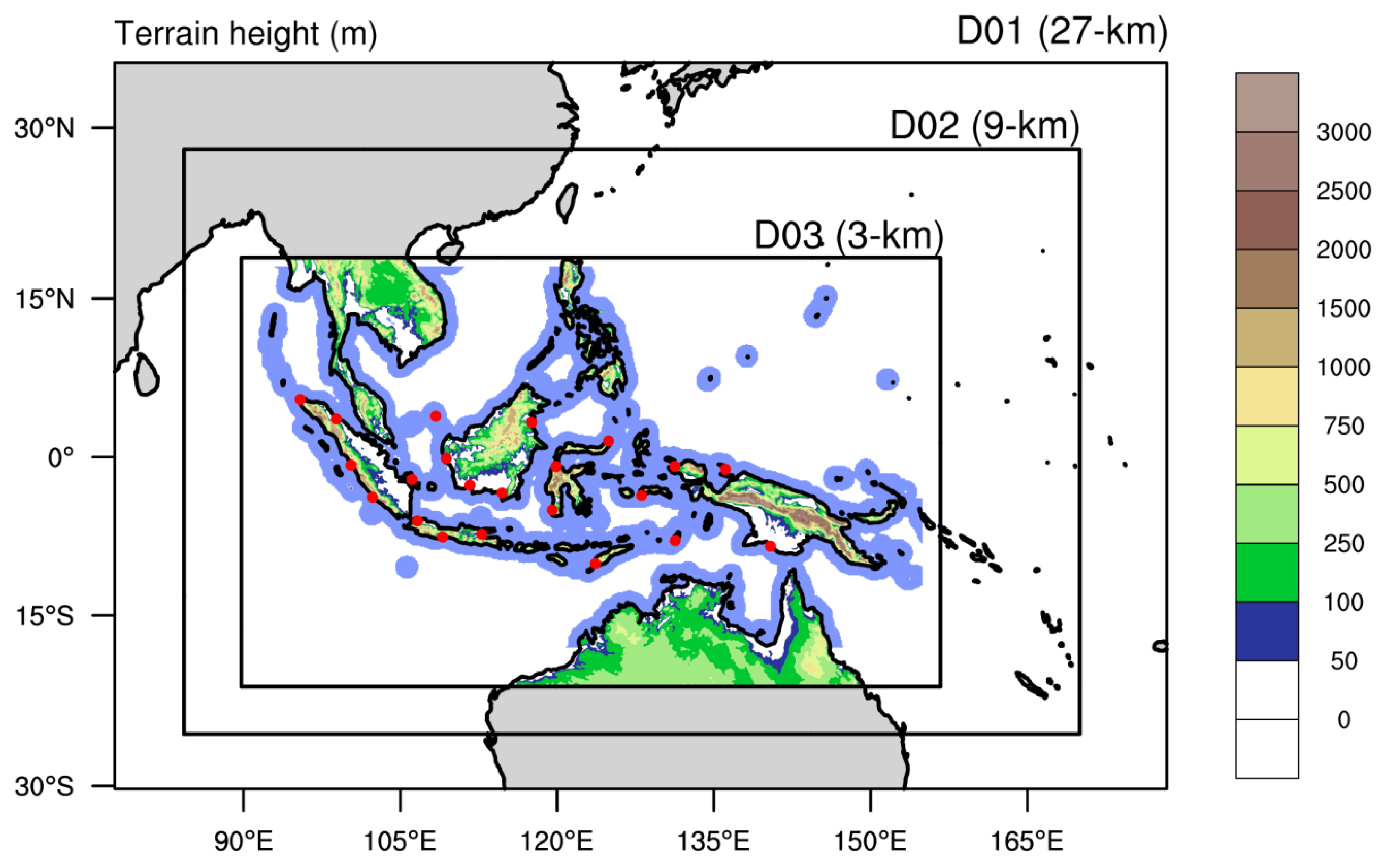
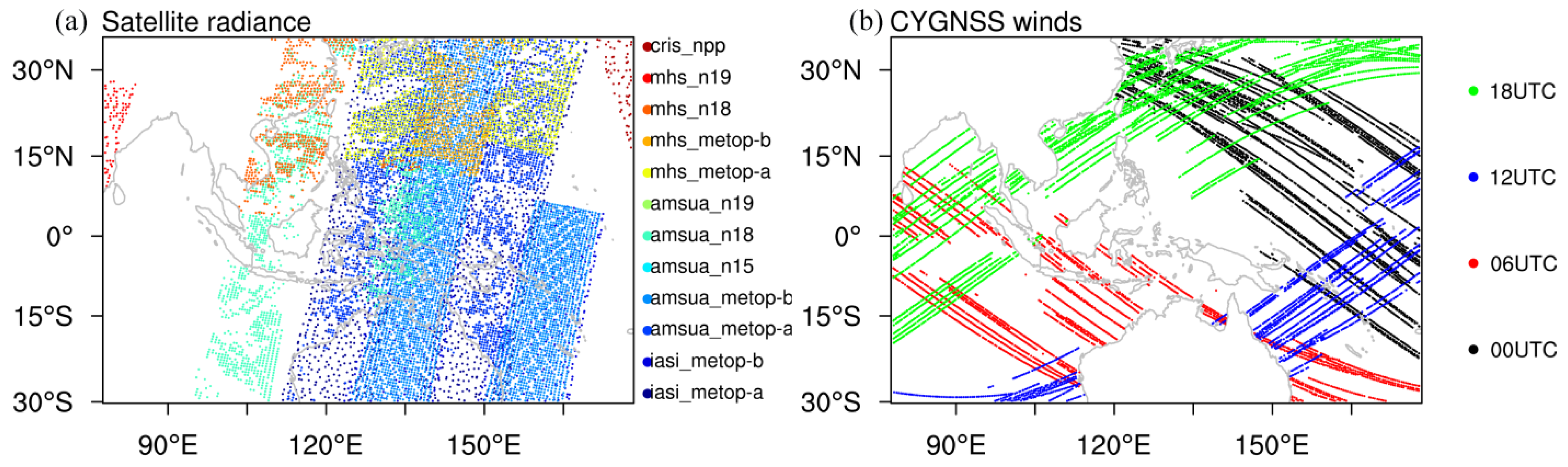
2. Model, Data Assimilation System, and Experiment Configuration

Simulations were conducted with an advanced research version of the Weather Research and Forecasting model (i.e., WRF-ARW) v4.0 [28]. Three-level nested domains were used (Figure 1) with horizontal resolutions of 27 km, 9 km, and 3 km, respectively. The domains were centered on central Indonesia and cover a large portion of the MC region. All model domains have 33 vertical levels, with a model top of 50 hPa. A 5 km Rayleigh damping layer from the model top was used to minimize the reflection of upward-propagating gravity waves generated by convection. The physical parameterizations included the new version of the Rapid Radiative Transfer Model (RRTMG) for longwave and shortwave radiation schemes, the Noah land surface model, and the Yonsei University (YSU) planetary boundary layer (PBL) scheme. The YSU PBL scheme was used in conjunction with the fifth-generation Mesoscale Model (MM5) surface layer scheme. Cloud microphysics processes were represented with the WRF Single-Moment 6-Class (WSM6) scheme. Sub-grid convection in the 27 km and 9 km domain was parameterized by the New Tiedtke cumulus scheme. The innermost domain (d03) was considered at a convection-permitting scale, and moist processes were treated explicitly. The blue-shaded area in Figure 1 shows the coastal ocean region (120 km offshore area) in later analysis.

For the control simulation, model initial and boundary conditions were provided by the National Centers for Environmental Prediction (NCEP) Final analysis (FNL) and forecast product at 0.25° × 0.25° resolution, with lateral boundary conditions updated every 6 h. Sea surface temperatures for all domains were prescribed daily from the NCEP real-time global (RTG) analysis at 0.083° × 0.083° resolution. For the data assimilation experiment, the NCEP Gridpoint Statistical Interpolation (GSI)–based hybrid ensemble–three-dimensional variational (3DEnVar) assimilation technique was employed. The cost function of the hybrid GSI 3DEnVar system had two terms: the background and observational error terms.

$$\mathrm{J}\left(\mathit{x}, \mathbf{\beta }\right)=\frac{1}{2}{\left({\mathit{x}}_{\mathit{b}}-\mathit{x}\right)}^T{\left({\alpha }_1{B}_{\mathbf{1}}+{\alpha }_2{B}_{\mathbf{2}}\right)}^{-1}\left({\mathit{x}}_{\mathit{b}}-\mathit{x}\right)+\frac{1}{2}{\left[{\mathit{y}}_{\mathbf{0}}-\mathrm{H}\left(\mathit{x}\right)\right]}^T{R}^{-1}\left[{\mathit{y}}_{\mathbf{0}}-\mathrm{H}\left(\mathit{x}\right)\right]$$

(1)

In the background error term (the first term in Equation (1)), $\mathit{x}$ is the analysis, and ${\mathit{x}}_{\mathit{b}}$ is the first guess, namely a 6 h WRF model simulation. The hybrid background error covariance matrix consists of a prescribed static part $B_{\mathbf{1}}$, and a flow-dependent part $B_{\mathbf{2}}$. The weighting factors of these two portions are 0.2 (${\alpha }_1$) and 0.8 (${\alpha }_2$), respectively, according to suggestions from previous studies with operational settings [29,30,31,32]. The horizontal and vertical localization used for assimilation was 110 km and three grid levels, respectively. The flow-dependent portion was estimated by 80-member 6 h ensemble forecasts from the NCEP GSI 4DEnVAR system.

Data assimilation was conducted in d01 and d02 with a horizontal grid spacing of 27 km and 9 km. The simulation with 3 km spatial resolution in the innermost domain was initialized from the d02 analysis and used in subsequent analyses. The observations used for data assimilation were NCEP operational conventional and satellite products. Conventional data from NCEP Automated Data Processing (ADP) contained land surface, marine surface radiosonde, pibal, and aircraft reports from the Global Telecommunications System, profiler and U.S. radar-derived winds, and satellite-derived winds. The satellite observations were a subset of the Level 1b or higher-level satellite products used in the NCEP Global Data Assimilation System (GDAS; https://doi.org/10.5065/DWYZ-Q852, accessed on 5 February 2023). Figure 2a illustrates the sample data coverage for satellite radiances at 00 UTC 20 Jan 2018 at four synoptic times of the same day over domain 1. Observations show good coverage over the MC region. The study period of the simulation experiment was January 2018, which included the entire eastward propagation of MJO from the Indian Ocean to the West Pacific. Six-hourly cycled data assimilation was conducted in sequence between 00 UTC 1 and 00 UTC 31 January 2018 with assimilation of the NCEP ADP and routine satellite data. In accordance with early sensitivity experiments, the data thinning distance for satellite radiance was set to 60 km. All observations within a 6 h time window (i.e., [−3 h, 3 h]) were used for assimilation at a certain analysis time.

Results from the control simulation (CTL hereafter) were compared with the data assimilation experiment (ECN) to examine the impacts of data assimilation on rainfall features over the MC region. In CTL, the WRF model was reinitialized every day at 00 UTC. The forecast/simulation was extended for 30 h. In ECN, analysis was conducted at four consecutive times (00 UTC, 06 UTC, 12 UTC, and 18 UTC) each day. The model forecasts ran for 30 h at 00 UTC and were compared with CTL. The first 6 h of forecasts in all forecast/simulation experiments were considered a spin-up period and were not used for diagnoses. Results were analyzed for the period 00 UTC 1 January–06 UTC 1 February 2018.

3. Fit of Analysis and Forecasts to Observations

To check the quality of regional analysis with data assimilation, verification was conducted by comparing the sounding data and the ERA5 hourly reanalysis. All sounding stations used in this comparison are shown in Figure 1. The ERA5 hourly reanalysis dataset from the European Centre for Medium-range Weather Forecasts (ECMWF) was used for reference, which is available at 0.25° spatial resolution. Figure 3 shows the root-mean-square error (RMSE) of the analysis fit to the available sounding observations averaged for 00 UTC each day over the experiment period. CTL generally shows comparable errors with ERA5 or even larger errors for temperature and dew point. The analysis from ECN fit the observations more closely than those from CTL and ERA5, especially for wind observations. Although the fit of the analysis to the assimilated observations is not a measure of the accuracy of the analysis field, the analysis tends to fit the observation conditions at the initial forecast time. Usually, conventional surface observations have greater temporal and spatial coverage (about 200 stations available with a 6 h time interval) than sounding observations. The RMSE fit of the 6 h forecasts from each assimilation cycle in the ECN experiment and the corresponding time in CTL for surface variables against surface observations was computed (

Table 1. The RMSE and BIAS of surface variables against surface observations averaged over the whole experiment period.

Experiment		Air Temperature (°C)	Specific Humidity (g kg−1)	Wind Speed (ms−1)	Wind Direction (deg)
RMSE	CTL	1.96	1.63	2.78	66
	ECN	1.83	1.43	2.75	68
BIAS	CTL	−0.14	−0.58	1.22	8.90
	ECN	−0.01	−0.36	1.35	0.25

). The forecasts produced by ECN show a smaller RMSE and BIAS in terms of temperature and dew point, and a comparable RMSE and BIAS for horizontal winds (wind speed and direction). The comparison result implies that regional data assimilation for the simulation over the MC region is effective. The lack of distinct wind improvements implied that there was still room for other assimilation methods to better handle surface data over complex terrain (e.g., [33]) However, these consistent improvements in the assimilation experiment encouraged us to analyze the model results and further investigate the physical aspects of precipitation features.

4. Precipitation

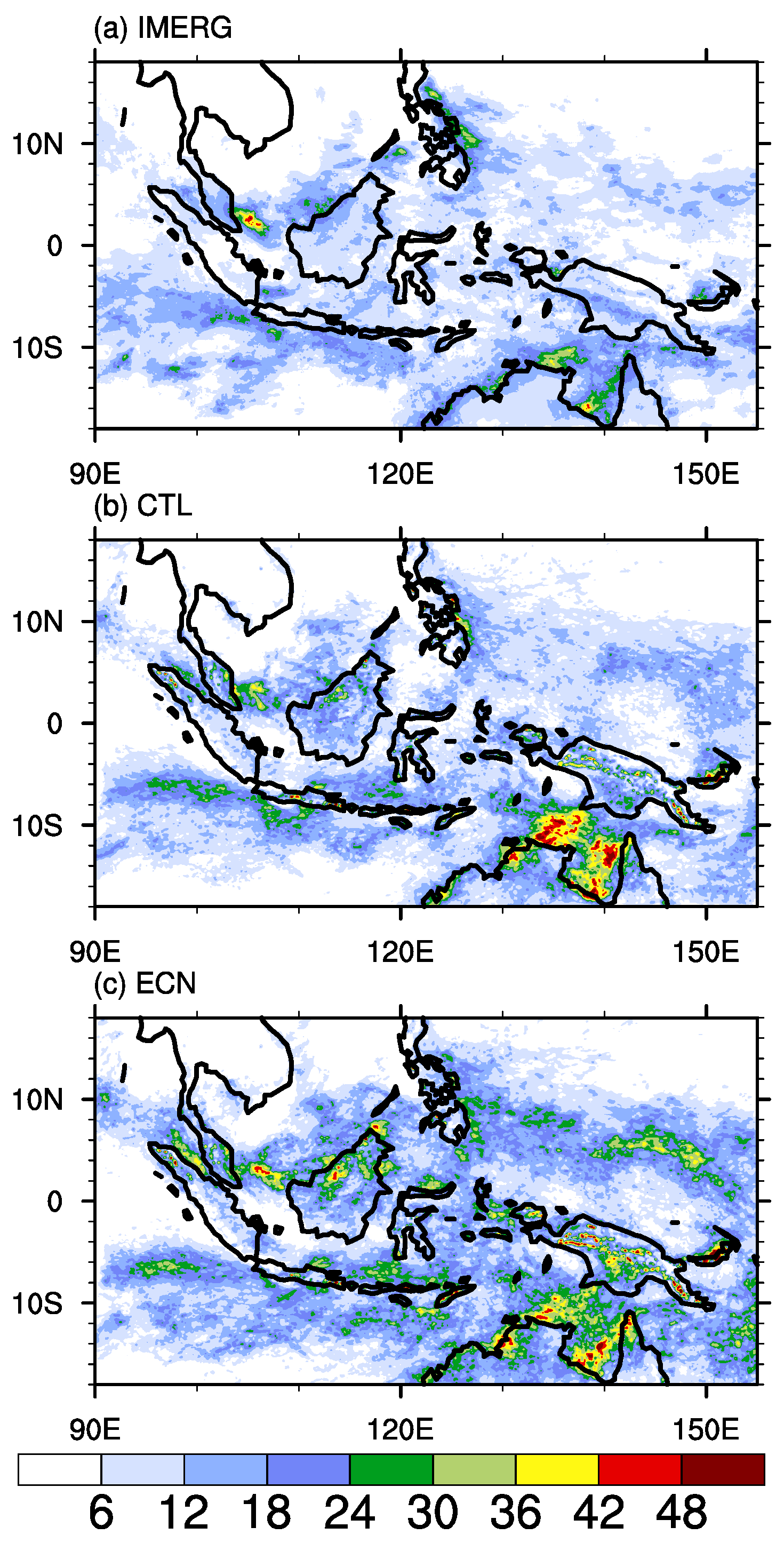
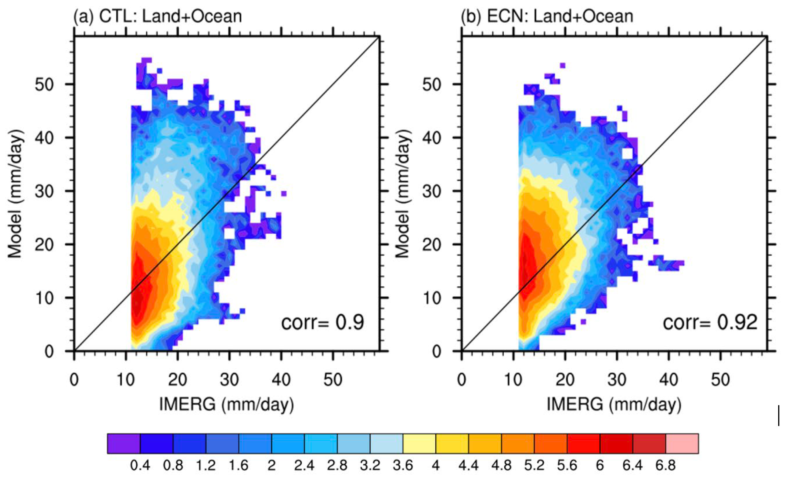
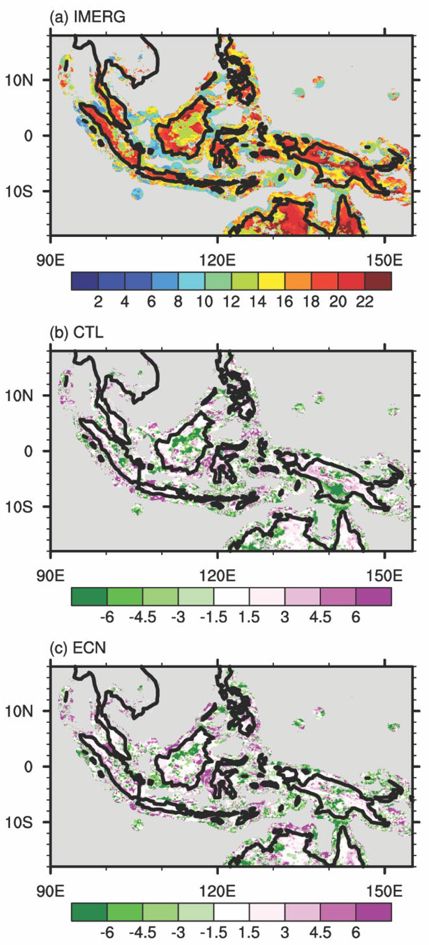
4.1. Mean Precipitation Features

Precipitation evaluation was conducted by comparing the simulations with the Integrated Multi-satellitE Retrievals for GPM (IMERG) precipitation estimates [34,35,36]. The IMERG precipitation product is available on a 0.1° × 0.1° grid starting from June 2000, and its time interval is 0.5 h. The satellite-estimated mean precipitation over the whole region for the period of 1–31 January 2018 is shown in Figure 4a. Most of the precipitation is concentrated along the coasts, as well as in some inland high-altitude areas, such as over New Guinea. Notable precipitation maxima occur near the concave coast of northern Australia, which may be associated with Australian summer monsoon lows [37]. The corresponding precipitation rate from CTL (Figure 4b) shows similar overall features to the satellite data. However, there is a distinct overestimation of rainfall maxima over the northern offshore region of Australia. The ECN experiment shows an improvement in precipitation maxima (Figure 4c), although with a slightly higher simulated intensity over much of the region, especially over the scattered islands in the West Pacific. All experiments were forced by daily updated GFS lateral boundary conditions and observed SST analysis, and the MJO signal embedded in the models is supposed to be the same as the observations on any given day. The rainfall anomaly by MJO phase shows a similar spatial pattern in both CTL and ECN (not shown). The eastward propagation of large-scale precipitation is well resolved in model simulations over the MC region.

A more quantitative comparison of simulated precipitation is presented in Figure 5. For the areas of evident precipitation in the IMERG product (using a threshold of 12 mm/day and means greater than 0.5 mm/h; this value was also used for large-scale precipitation tracking in [38]), for ECN, the assimilation shows better agreement with IMERG than CTL, as indicated by the higher uncentered pattern correlation. Specifically, ECN shows better concentration, and the high-density center is more symmetrically distributed on both sides of the 1:1 agreement line. The bias of the overall underestimated precipitation has been modulated (Figure 5b).

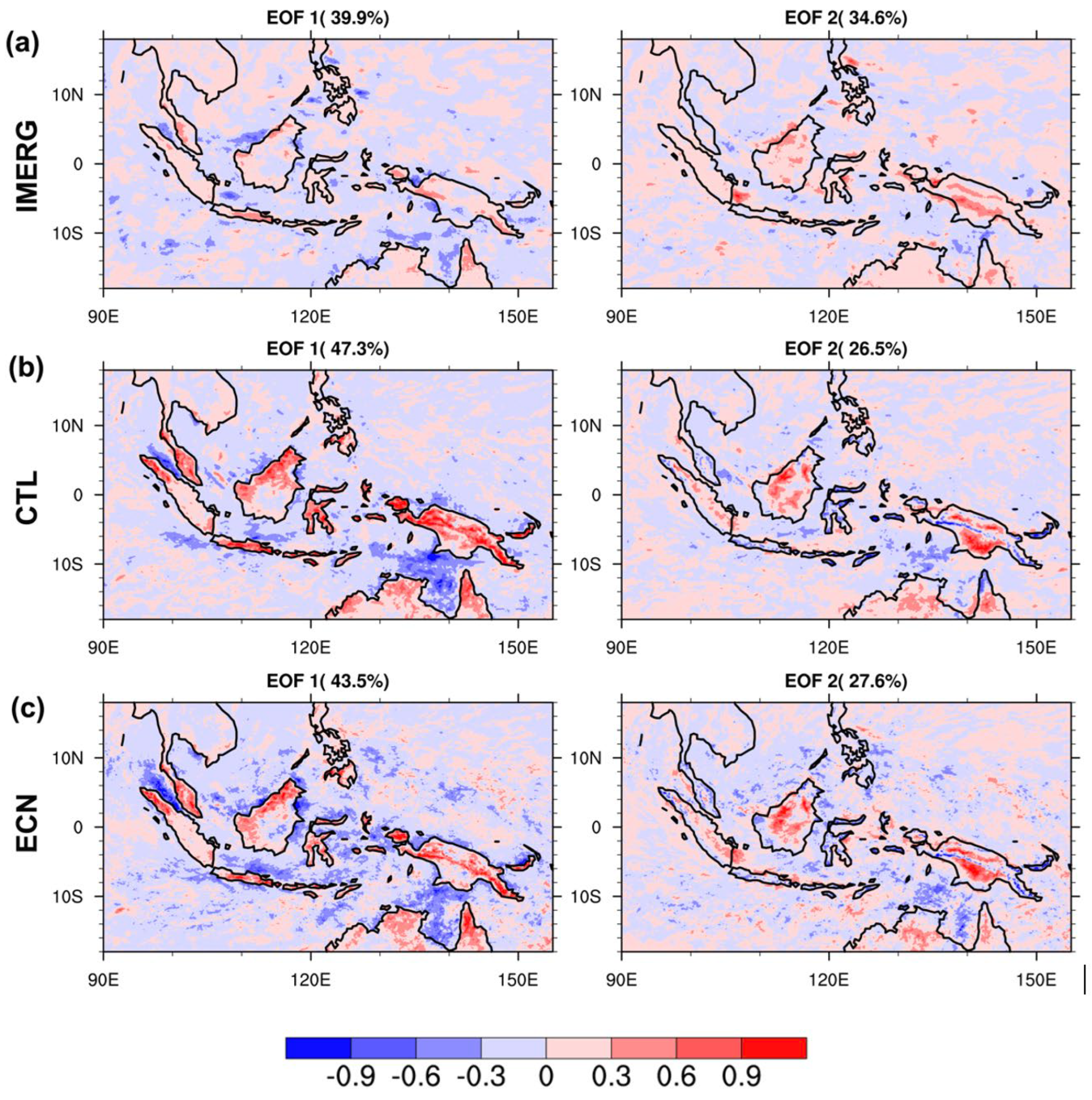
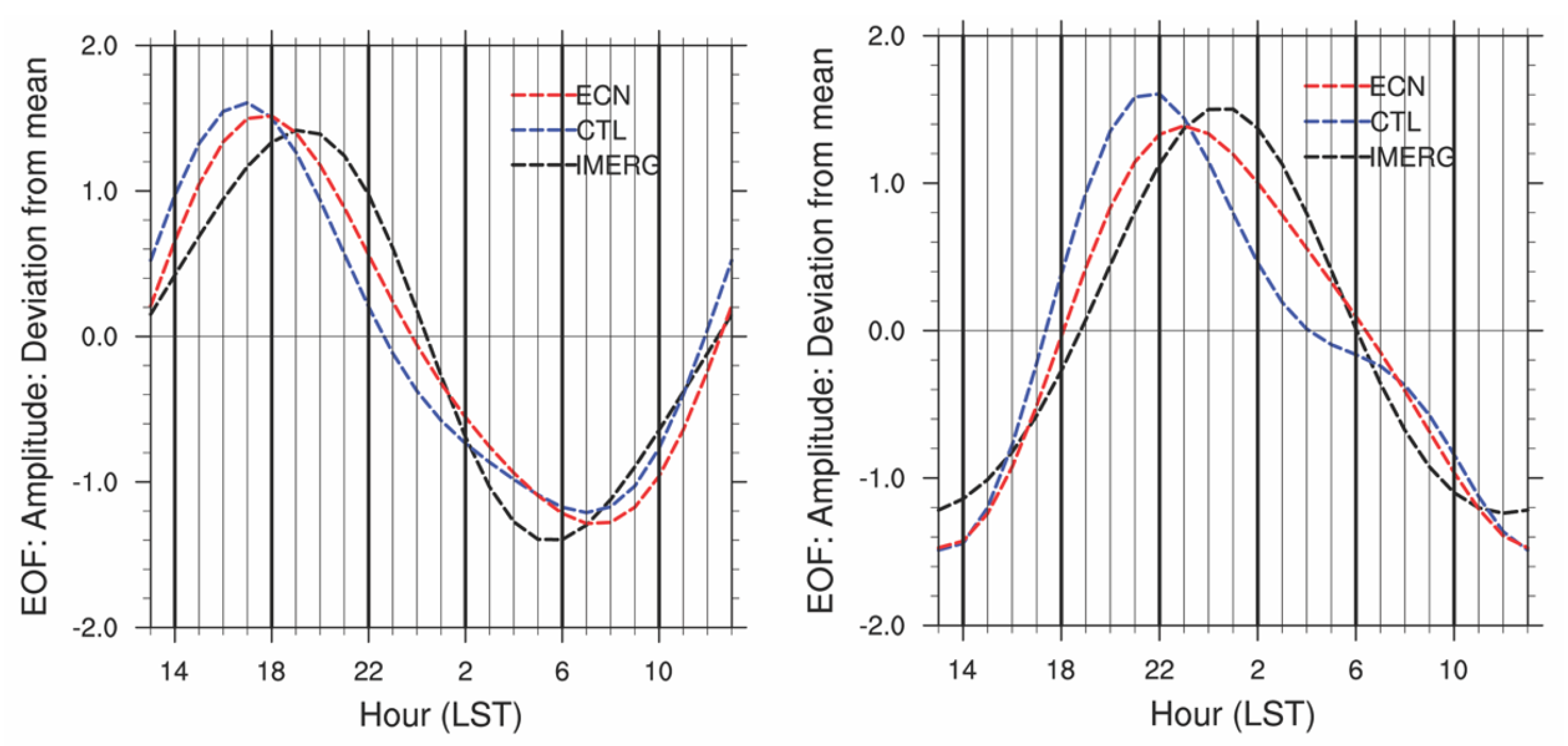
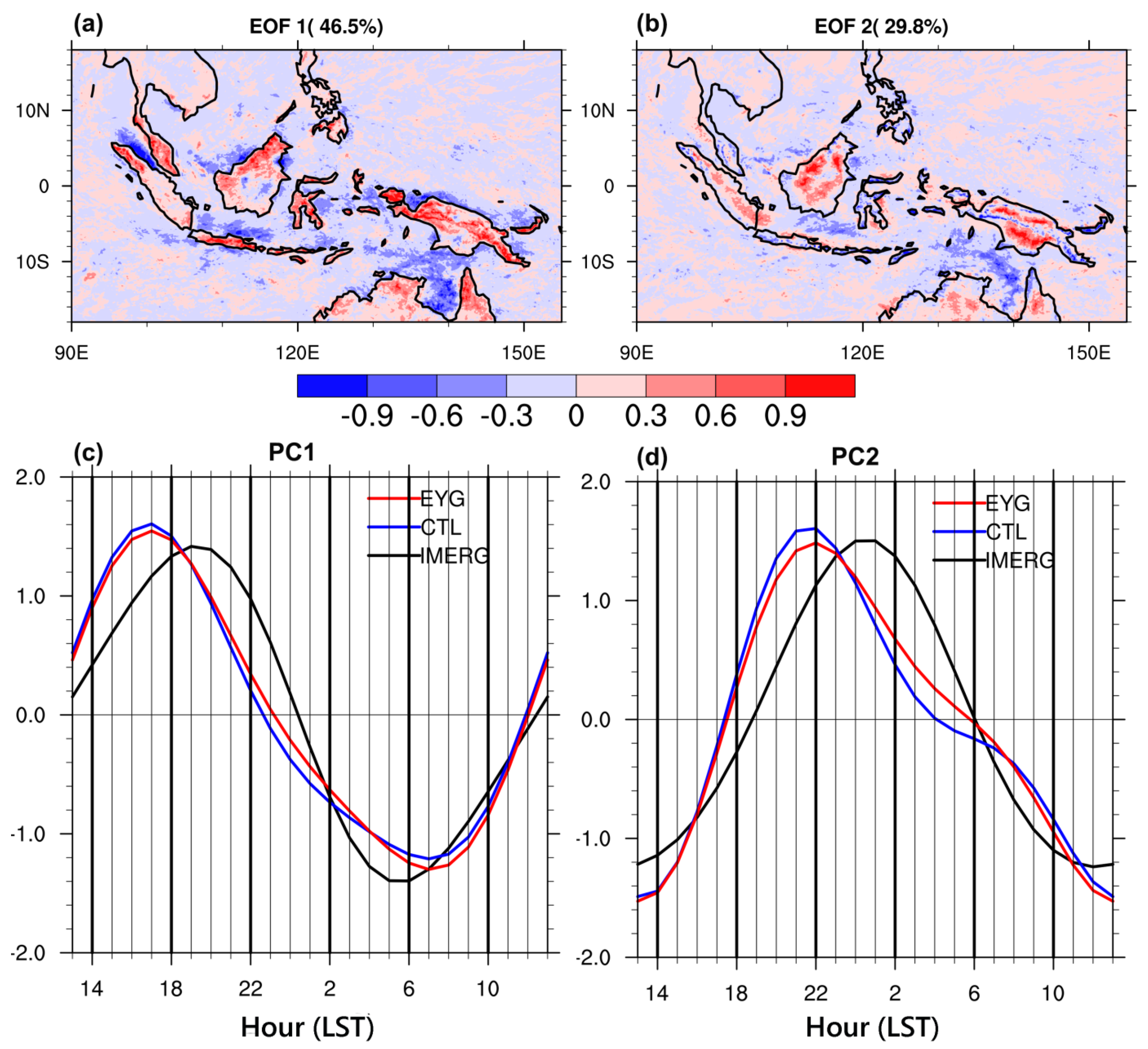
4.2. Major Components of the Diurnal Cycle of Precipitation

Ground validation demonstrates the unprecedented ability of IMERG to capture the diurnal cycle of global precipitation [35]. The mean diurnal cycle is constructed by averaging all values at a particular time of day, and the daily mean is constructed by a series of such composite averages. To filter out the noise and other possible modes of sub-semidiurnal disturbances in the analysis, a low-pass filter [35] was applied to the mean precipitation rates through a fast Fourier transform, discarding components with frequencies above two cycles per day. First, to identify the dominant components of diurnal variability, an empirical orthogonal function (EOF) decomposition of the hourly mean precipitation field was performed over the whole tropical region, which consisted of spatial patterns and the corresponding time series (principal components, PCs). In addition, for each grid point in the simulation domain, the least squares method was used to fit a harmonic curve to explain the overall diurnal cycle of each grid point using the following formula [19]:

$$p=\overline{p}+A\cos \left\{\frac{2\pi \left(t-t_{\varnothing }\right)}{24}\right\}$$

where $\overline{p}$ is the mean precipitation rate, $t$ is the time in hours, $A$ is the amplitude of the diurnal harmonic, and $t_{\varnothing }$ is the time of the precipitation peak. We then converted the UTC time to local solar time (LST) based on longitude.

To clearly identify the main modes of variability in the diurnal cycle over the whole domain, we conducted an EOF analysis with low-filtered hourly mean precipitation for the whole simulation period. The first two EOF modes from both the IMERG dataset and the model simulations are shown in Figure 6 and Figure 7, with their spatial patterns and corresponding time series PCs. The two modes explain approximately 70% of the variance in total. We can restrict our analysis to these for the overall features of the diurnal cycle.

The first EOF mode (first column, Figure 6) shows that a spatial pattern marks mainly the dominant land–sea contrast along the coast of major islands in the MC region; it also reveals some weak local-scale mountain-valley contrast over sloping terrain (e.g., an alternating pattern over southern Sumatra, eastern Borneo, and New Guinea). In CTL, a large percentage of afternoon peaks over land are reproduced, but with stronger amplitude, which implies that the basic diurnal forcing is too strong [20]. In ECN, the amplitude decreases slightly, and the alternating spatial pattern over the major islands is more consistent with IMERG. Over the ocean, both experiments tend to overestimate the negative modes to some extent and show similar spatial pattern correlations with IMERG over the coastal region (indicated in Figure 1). Meanwhile, in some regions (e.g., the Arafura Sea), ECN shows slightly better spatial patterns. In the corresponding PC1 (Figure 7a), the observed afternoon precipitation peak develops between 19 and 20 LST, and the morning peak occurs between 5 and 6 LST. The two experiments present an early afternoon peak and a late morning peak, but it is notable that the situation of the early afternoon peak is improved in ECN, which narrows the gap to only about one hour. Meanwhile, a slightly larger amplitude of afternoon precipitation and a smaller amplitude of morning precipitation in CTL tend to be adjusted closer to the IMERG dataset in ECN.

The second EOF mode (second column, Figure 6) demonstrates mainly a spatial pattern of late evening maximum precipitation over land. The main peak of EOF2 lags behind that of EOF1 by about 5 h (nearly a quarter of the diurnal cycle); this spatial pattern shift between the two modes indicates a propagation feature of the diurnal cycle, as suggested in a previous study [39]. The pronounced propagation of rain peaks can be found around the northeastern coast of Borneo, the coast of Sulawesi, the mountains of New Guinea, and the Cape York Peninsula. The much weaker scattered peaks along the eastern coast of southern Sumatra and Lampung in EOF1 also merge and strengthen during the eastward propagation, so peaks on the western edge of the Java Sea can be seen. In both experiments, the rain peak on the northwestern coast of Borneo is less than the observation, which indicates no effective propagation from the land into the coastal sea. However, a detailed comparison between model simulations suggests that propagation southward from the central ridge of New Guinea, offshore migration around Sulawesi, and eastward propagation on the western edge of the Java Sea are better resolved in ECN. The PCs for the second mode show that an evening peak develops at 21 LST in CTL, which leads the observations by about 4 h. Obviously, ECN dramatically improves this situation. It narrows the timing gap down to a one-hour difference from the IMERG dataset, which means about a 75% reduction of the time biases in the model simulation.

Note that the diurnal phases depicted in all these observations and simulations generally lag those of previous statistical analyses for a long period (e.g., [39]). This difference suggests that an MJO-enhanced phase could modulate the diurnal cycle of precipitation over the MC and shift it to a later time.

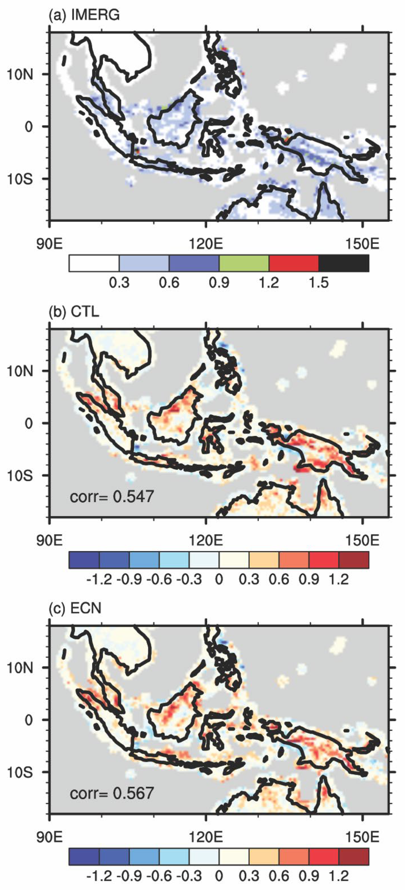
4.3. Harmonic Analysis of the Diurnal Cycle of Rainfall

To identify the local diurnal cycle of precipitation at each location in the whole area, harmonic analysis was performed based on the low-pass-filtered mean rainfall rate between the IMERG dataset and model simulations. The results are presented in Figure 8 and Figure 9. The amplitude and phase of the diurnal harmonic maps in the model simulations are shown as the differences from the IMERG dataset. A negative value indicates that the model exhibits smaller amplitudes (later peaks), while a positive value corresponds to larger amplitudes (early peaks). We noticed that the early morning signal over the open ocean (>120 km from the coast) is much noisier than that over land, which could be due to the influences of weaker convection or artificial diurnal variabilities [35]. In the following analysis, we focus on the coastal ocean (<120 km from the coast, indicated by blue shaded area in Figure 1)) and land region.

Broadly speaking, the observed precipitation over the MC is greatest over the islands and some of the surrounding coastal seas (Figure 8a). This general spatial pattern is reproduced in all experiments with a much larger amplitude. However, in the assimilation experiment, the area with a large deviation is slightly reduced, and the spatial pattern is more consistent with the IMERG data (as indicated by the higher correlation coefficients). In Figure 9, considering the high uncertainty of the harmonic phase in the case of much weaker amplitude when using the least-squares fitting method, we show only the area in which the amplitude is larger than 0.1 mm/hour. The phase of the diurnal cycle is such that, over the inland region, the maximum precipitation spans from early afternoon to late evening, whereas over the coastal ocean, it can last from the morning to the afternoon (Figure 9a). The differences of all model simulations from the IMERG data indicate that ECN effectively reduces the area of the lag region over the land in CTL, especially over Borneo and New Guinea. ECN shows slightly better results.

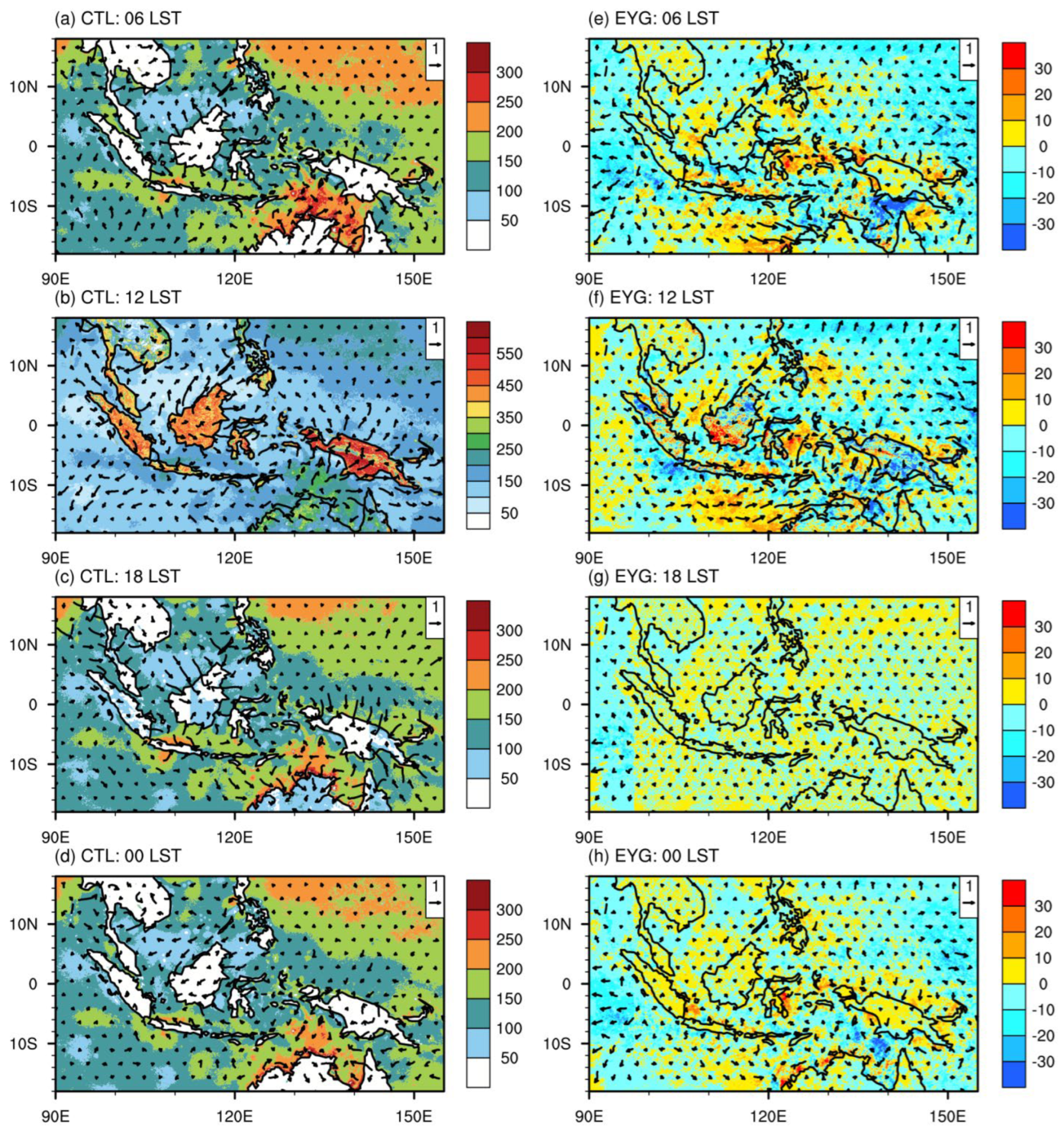
5. Mean Diurnal Cycle of Thermodynamic Conditions

The intensity of convective activity is closely related to the atmospheric thermodynamic conditions before convection occurs. The mean diurnal cycle of potential temperature and water vapor mixing ratio were analyzed. Then, the associated surface heating and low-level water supply were examined. Since the amplitude of the diurnal cycle of precipitation over the open ocean (>120 km from the coast) is negligible, here we focus on the coastal sea (blue shading in Figure 1) and the lowlands, defined as regions below 250 m above mean sea level (MSL) over the MC region.

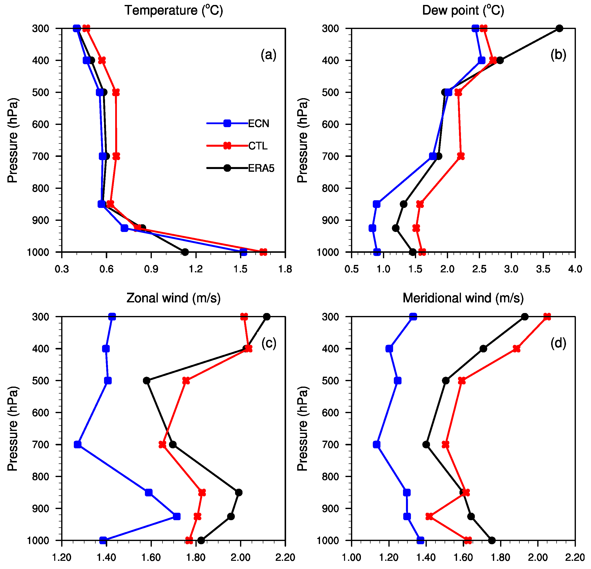
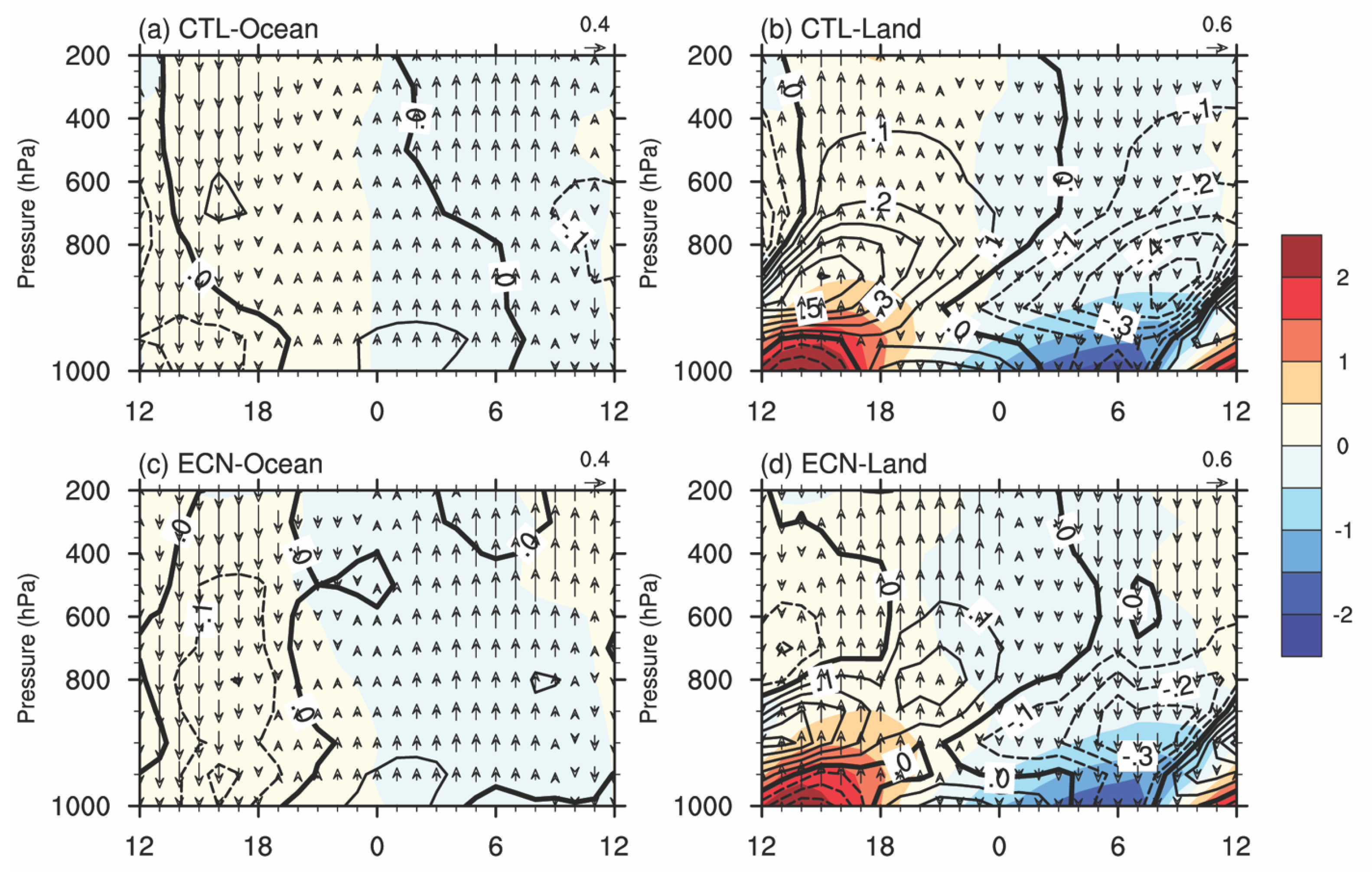
5.1. Vertical Thermodynamic Profile

Figure 10 shows the mean diurnal cycle of the potential temperature and water vapor mixing ratio anomalies (i.e., the values after removing the daily average) and associated vertical velocity averaged over the coast and lowlands, respectively. For the potential temperature, in general, a positive anomaly occurs during the daytime and a negative anomaly at night, which is consistent with the diurnal cycle of solar insolation. Over the ocean, all model results show a much weaker amplitude, and the sign change of the anomaly from positive to negative in CTL occurs around 23 LST at all pressure levels, whereas in ECN, the sign change in the higher troposphere lags behind that in the lower troposphere; that is, the negative anomaly in the higher troposphere appears early. This slight profile shift could lead to an increase in thermal instability during the night over the ocean, providing a more favorable environment for convection. Over the lowlands, the amplitude of the diurnal cycle of the potential temperature anomaly is much more obvious below 850 hPa, and the maximum is above 1 °C. Such features could be regarded as the difference in heat capacity between land and sea. Particularly near the surface, the strong positive daytime anomaly and the negative nighttime anomaly (absolute value greater than 1 °C) initiate at the surface level and then gradually spread upward to the 900 hPa level. Therefore, the sign change of the anomaly between the 800 and 900 hPa levels lags behind that of other pressure levels in all simulations. The significant difference among experiments is that there is a relatively small magnitude of anomalies in ECN, and the timing of this strong anomaly initialization in this experiment slightly lags behind that in CTL. This warm and cold anomaly reduction and time change in the assimilation experiment implies that the strength of the thermal instability will decrease in the lower troposphere and will be less favorable for convection initiation over land, and precipitation will show up later.

The mean diurnal cycle of the water vapor mixing ratio presented in Figure 10 also shows a distinct sign change of the anomaly with day and night. The time of transition between positive and negative anomalies is not consistent over the coastal ocean in two experiments. Over the lowlands, the timing of sign change in the lower troposphere (950 to 800 hPa) is also different from that of the other layers The magnitude of the anomaly over the coastal ocean is much weaker than that over the land. Looking in depth at these anomaly profiles among all the experiments, over the coastal ocean, the positive anomaly in the lower troposphere starts in the evening (around 18 LST), lasts a short time in CTL, and ends the next morning (6 LST), and the initial positive anomaly may be due to the descending contribution from high altitudes (slanting isolines). In ECN, the positive anomaly ends at noon the next day and leads to an increase in the water vapor contribution from the ocean surface. Over the lowlands, the positive and negative anomalies in the lower troposphere are much stronger in CTL than in ECN, and they develop at a higher altitude over time, up to 500 hPa. The positive anomaly gradually weakens after 18 LST in CTL, while it reintensifies in ECN, which could lead to late evening precipitation. Meanwhile, it is noticeable that the afternoon negative anomaly near the surface synchronizes with the strong temperature anomaly in ECN and remains longer than that in CTL, which indicates a lower contribution of precipitation evaporation to near-surface humidity due to the decrease in precipitation in the early afternoon.

In addition, the corresponding variation of vertical velocity in Figure 10 also has several noteworthy characteristics. First, diurnal variations in descending and ascending motion exist over both the coastal ocean and the land, but the phase changes are opposite and stronger over the land.

Second, over the ocean, the early ascent in the lower troposphere (below 800 hPa) was initiated at around 19 LST. Compared with CTL, more layers in the middle and upper levels (above 700 hPa) in ECN indicate a sinking motion. This circulation shift could be beneficial for water vapor collection in the lower troposphere. Third, the ascending layer over the land in the afternoon starts at a slightly later time in ECN and continues until around 23 LST in the middle and upper levels, while it ends at 19 LST in CTL, which may suppress late evening precipitation.

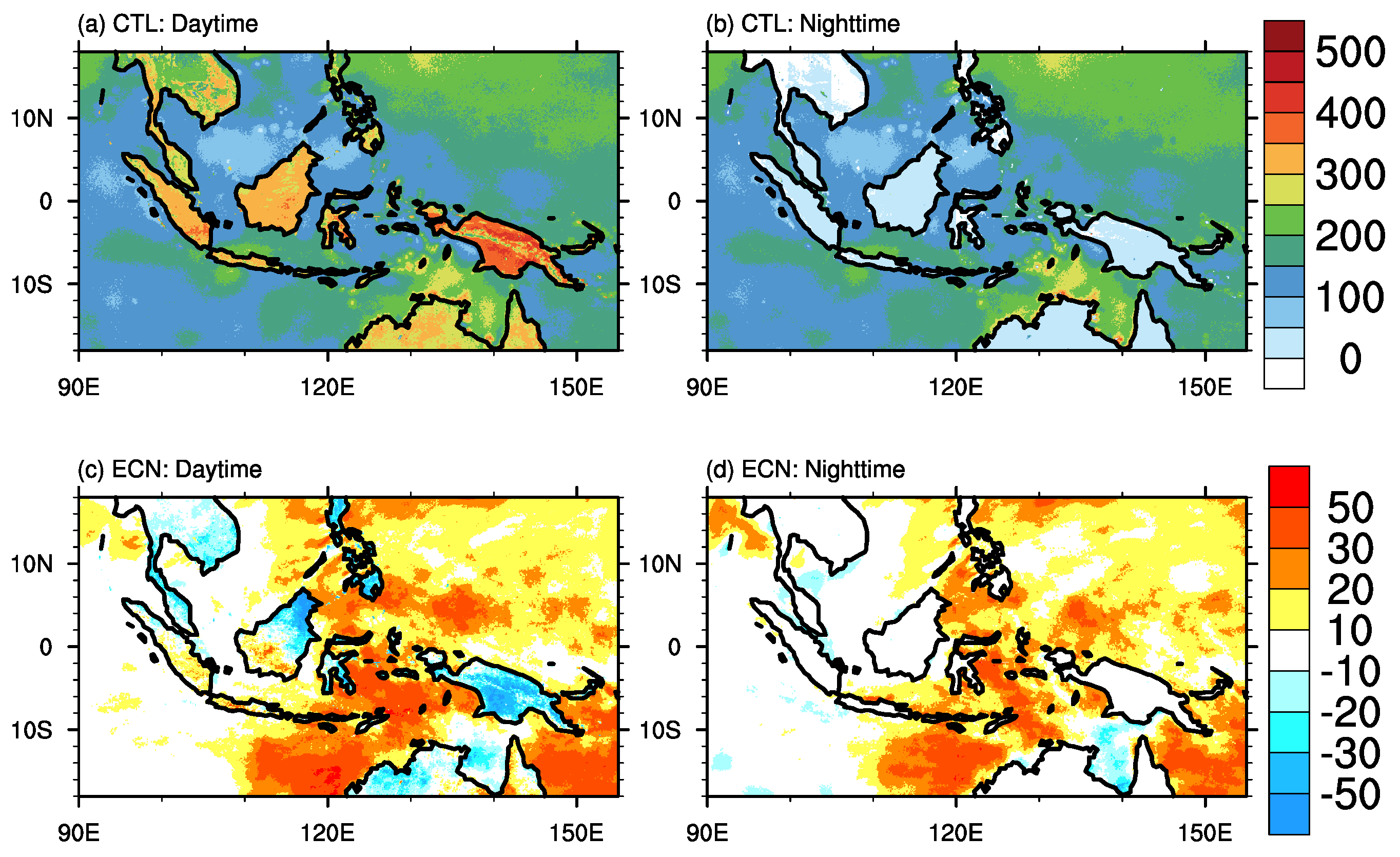
5.2. Surface Heat Fluxes

Figure 11 compares the spatial distribution of mean surface enthalpy flux during the daytime (8–20 LST) and nighttime (20–8 LST). Results show that surface diabatic heating over the land is stronger during the daytime than during the nighttime, while the diurnal variation over the ocean is weak. Although there is a slight increase in heating over southern Sumatra, Java, southern Borneo, and the southern coast of the Gulf of Carpentaria, daytime surface diabatic heating over most of the land surface is reduced in ECN compared with CTL, with less difference during the nighttime. Over the ocean, the diabatic heating in ECN is generally much stronger than that in CTL during both daytime and nighttime, with the exception of a constant reduction over the Arafura Sea. Both sensible heat flux and latent heat flux show similar adjustment patterns, but latent heat flux exhibits a dominant magnitude, especially over the ocean (not shown). These results correspond well to the smaller magnitude of the potential temperature anomaly near the land surface in ECN.

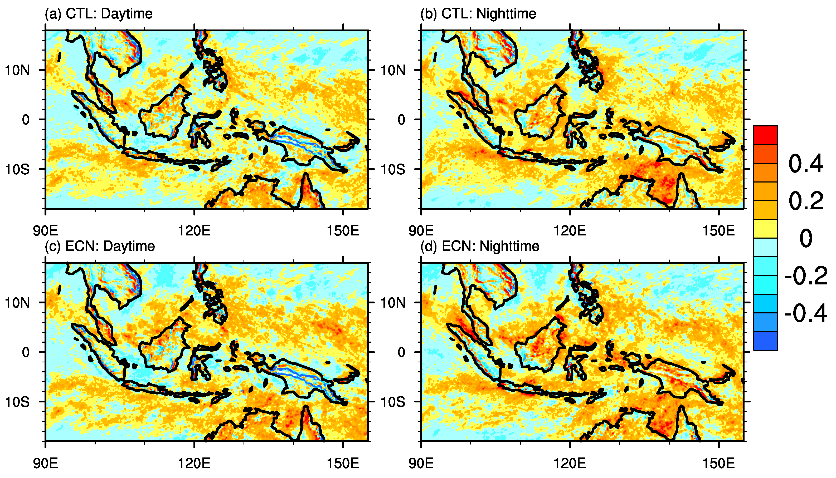
5.3. Low-Level Moisture Supply

To examine the difference in the diurnal variation of the low-level moisture supply in all experiments, we calculated the total horizontal moisture flux convergence, vertically integrated between the surface and 700 hPa. The formula is as follows:

$$VIMFC=-{{\displaystyle \int }}_{p=700}^{ps}\left[{\nabla }_p·\left(\overrightarrow{U}q\right)\right]\frac{dp}{g}$$

(2)

where $VIMFC$ is the vertically integrated moisture flux convergence (g m⁻² s⁻¹), ${\nabla }_p$ is the horizontal divergence in pressure coordinates, $\overrightarrow{U}$ is the horizontal wind vector (m s⁻¹), and $q$ is the specific humidity (g kg⁻¹), g is the gravitational acceleration (m s⁻²). Figure 12 shows the mean spatial pattern of VIMFC during the daytime and nighttime in all experiments. Over the ocean away from the islands (>120 km from the coast), there is less diurnal variation in VIMFC, and ENC generally has a slightly larger magnitude of moisture convergence, which accounts for the increase in total precipitation over the ocean. Over the islands and adjacent ocean, a distinct diurnal variation in VIMFC and a difference between experiments can be found. Especially along the northwest coastline of Borneo, daytime moisture flux divergence and nighttime moisture flux convergence exist in CTL, while ECN tends to adjust to moisture flux convergence during the daytime and a stronger moisture convergence can be observed during the nighttime. This implies a higher possibility of coastal precipitation in ECN. Over Borneo and New Guinea, ECN shows a wider range of moisture flux divergence during the daytime and a stronger moisture flux convergence during the nighttime, which could contribute to the later evening precipitation over the land. It is important to note that the smaller magnitude of VIMFC over the Arafura Sea also agrees well with precipitation adjustments in ECN.

6. Impact of CYGNSS Wind Data

Overall, in ECN, the mean spatial distribution of precipitation is better resolved compared to CTL, implying the benefit of regional data assimilation versus the original global GFS analysis. To further examine the data assimilation impact on the simulation of diurnal precipitation over the MC region, we conducted additional data assimilation with NASA research satellite CYGNSS data. CYGNSS was launched to measure ocean surface winds between approximately 38°N and 38°S latitudes ([27,40,41] see sample CYGNSS data in Figure 2b). It provided a relatively frequent revisit time and was able to monitor the rapidly evolving wind over the MC region [36]. The application to the prediction of tropical cyclones suggests a better track and intensity forecast from the assimilation of CYGNSS data into NWP models [42,43], and CYGNSS data assimilation appears to have a positive impact on the wind field in tropical convection [44].

We first combined CYGNSS data with all observations used in ECN. Through EOF decomposition of the mean diurnal cycle of rainfall, the new data assimilation experiment shares almost the same spatial pattern and phase shift, and the data impact of CYGNSS is less noticeable. This is probably because the CYGNSS data sample size is much smaller than the total amount of other data at each assimilation cycle, and it is limited to the surface layer of the ocean. Considering this issue, by isolating the impact of CYGNSS wind speeds, we conducted an additional assimilation experiment (experiment CYGNSS; EYG), which uses the same configuration as the previous data assimilation experiment but assimilates only CYGNSS satellite-derived ocean surface wind speeds at each analysis cycle. As a result, the monthly mean spatial distribution in this simulation does not show a distinct improvement, with a slightly greater rainfall maximum than in CTL (not shown). However, comparisons of the mean diurnal cycle show an apparent difference from CTL (Figure 13). The mean features in this assimilation experiment reproduce the transition of the two spatial EOF modes from CTL to the assimilation simulation described above. The corresponding PCs suggest that the phase of the rainfall rate from this assimilation experiment is relatively shifted toward the observation. Especially in PC2, the phase lead of peak rainfall is reduced.

Moreover, the composite diurnal cycles of surface latent heat flux and 10 m wind in CTL and EYG are shown in Figure 14. In CTL, there are evident diurnal variations in both surface latent heat flux and surface winds (Figure 14a–d). At 06 LST, the major islands, such as Sumatra, Borneo, New Guinea, and northern Australia, are dominated by land breezes, and the latent heat flux over the ocean is relatively strong, especially in the Arafura. At noon (12 LST), the latent heat over the land significantly increases, and land breezes grow stronger. After that, the circulation over the coastal region turns to a sea breeze with a decrease in surface latent heat flux, and at 00 LST, the wind component crossing the coastline becomes weak, probably due to the small temperature difference between land and sea. Meanwhile, inland valley winds show up across the major islands, attributed to the steep topography, whereas in EYG (Figure 14e–h), during the whole period, the strength of the land breeze decreases slightly and the sea breeze increases. In general, the maximum value of latent heating over the land at noon has decreased and increased at other times of the day. This result indicates that data assimilation has an evident capability to modulate the surface diurnal variation of surface heating and winds and improve the diurnal cycle of rainfall over the MC. CYGNSS wind data by itself is also responsible for regulating the diurnal cycle.

7. Summary and Concluding Remarks

This study has demonstrated the impact of data assimilation on the mean spatial features and diurnal cycle of precipitation using cloud-permitting-scale numerical simulations with various available observations. The simulation with the WRF model focuses on January 2018 (study period), which corresponds to a convective MJO phase that propagated through the MC region, to investigate the ability of the numerical model to resolve the characteristics of precipitation modulated by forcing from the MJO active phase. Previous studies have noted that WRF model simulations usually struggle to reproduce the actual amount of precipitation and show the diurnal peak too early [20,45]. High-resolution simulations with grid spacing small enough to turn the convective parameterization off show some improvement in the initiation of convection and the diurnal cycle of precipitation (e.g., [21]). In this study, a set of WRF model simulations configured with one-way nested domains was performed. In the control simulation, the model reinitializes each day at 00 UTC, and no data are assimilated, while in the assimilation simulation, the observations are ingested within a 6 h analysis cycle. Our analysis focuses on results from a 3 km horizontal grid spacing domain.

First of all, the vertical profile of analysis from the data assimilation experiment (ECN) exhibits smaller errors against sounding observations, even better than the ERA5 reanalysis, and the forecasts still show better representation against surface conventional observations. This provides a fundamental reason to analyze simulated precipitation and possible causes of precipitation improvement in numerical models with data assimilation. The model-simulated precipitation shows better spatial agreement with satellite-estimated precipitation from IMERG in the assimilation experiment than in the control experiment. The bias of overall underestimation decreases over the ocean. The diurnal features of precipitation in the observations and models are identified by the first two EOFs, the corresponding PCs of which are in the time dimension. The first EOF represents precipitation variation, forced by insolation change with time, evolving over the land and sea, and the second EOF represents local nocturnal precipitation over the coastal ocean and inland areas of Borneo and New Guinea, which could result from interaction with MJO mesoscale convection. The first EOF of ECN is more consistent with the observation, although with a slightly larger magnitude over the coastal ocean. It effectively improves the variance over southern Sumatra and New Guinea in terms of the second EOF. A phase lead of both the modeled PC1 and PC2 compared to the observation in the control simulation is modulated in the assimilation experiments, especially ECN, with only a one-hour difference between the simulated results and the observation. The local diurnal cycle over the MC identified by harmonic analysis also suggests that it is more realistic in the assimilation experiment, especially for the timing of the precipitation peak during the day.

To investigate the thermodynamic environmental conditions needed for precipitation to occur, the mean diurnal cycle of thermodynamic profiles is examined over the coastal ocean and lowland areas in between control simulation (CTL) and data assimilation simulation (ECN). First, the strength of the diurnal cycle of the potential temperature and water vapor mixing ratio anomalies decreases in the assimilation in the lower troposphere over land but is slightly stronger over the coastal ocean. The out-of-phase vertical change in temperature and the longer duration of the positive moisture anomaly during the nighttime over the coastal ocean are responsible for the morning precipitation. The out-of-phase vertical shift in the positive temperature and the moisture anomaly over land during the daytime tend to trigger the precipitation later. The associated vertical motion is much stronger over both the coastal ocean and the land, and there is a relatively late transition of the ascending and descending motion in the middle troposphere. The corresponding surface heating comparison suggests that strong surface diurnal forcing generally decreases over the land surface and increases over the ocean, except for the Arafura Sea, where excessive precipitation in the control experiment decreases in the data assimilation experiment. Moreover, in the data assimilation experiment, the low-level moisture convergence decreases over the land and increases along the northwestern coast of Borneo during the daytime, while it increases over the land and decreases over the Arafura Sea during the nighttime. These adjustments succeed in bringing the characteristics of the simulated precipitation closer to observations.

Results from this study highlight the importance of data assimilation in improving the representation of precipitation over the Maritime Continent, especially for the diurnal cycle. The assimilation of CYGNSS data also shows some impacts on the diurnal variation of surface variables and benefits in the improved diurnal cycle of precipitation. However, these results are limited in scope, as they focus on only one period of the MJO active phase. Future work will emphasize more comprehensive studies with additional cases and a more advanced data assimilation system.

References

1. Gill, A.E. Some simple solutions for heat-induced tropical circulation. Q. J. R. Meteorol. Soc. 1980, 106, 447–462. [Google Scholar] [CrossRef]
2. Neale, R.; Slingo, J. The Maritime Continent and its role in the global climate: A GCM study. J. Clim. 2003, 16, 834–848. [Google Scholar] [CrossRef]
3. Ramage, C.S. Role of a tropical “Maritime Continent” in the atmospheric circulation. Mon. Weather Rev. 1968, 96, 365–370. [Google Scholar] [CrossRef]
4. Kikuchi, K.; Wang, B. Diurnal precipitation regimes in the global tropics. J. Clim. 2008, 21, 2680–2696. [Google Scholar] [CrossRef]
5. Vincent, C.L.; Lane, T.P. A 10-year astral summer climatology of observed and modeled intraseasonal, mesoscale, and diurnal variations over the Maritime Continent. J. Clim. 2017, 30, 3807–3828. [Google Scholar] [CrossRef]
6. Ichikawa, H.; Yasunari, T. Intraseasonal variability in diurnal rainfall over New Guinea and the surrounding oceans during austral summer. J. Clim. 2008, 21, 2852–2868. [Google Scholar] [CrossRef]
7. Ogino, S.Y.; Yamanaka, M.D.; Mori, S.; Matsumoto, J. How much is the precipitation amount over the tropical coastal region? J. Clim. 2016, 29, 1231–1236. [Google Scholar] [CrossRef]
8. Yokoi, S.; Mori, S.; Katsumata, M.; Geng, B.; Yasunaga, K.; Syamsudin, F.; Nurhayati, N.; Yoneyama, K. Diurnal Cycle of Precipitation Observed in the Western Coastal Area of Sumatra Island: Offshore Preconditioning by Gravity Waves. Mon. Weather Rev. 2017, 145, 3745–3761. [Google Scholar] [CrossRef]
9. Madden, R.A.; Julian, P.R. Detection of a 40–50 day oscillation in the zonal wind in the tropical Pacific. J. Atmos. Sci. 1971, 28, 702–708. [Google Scholar] [CrossRef]
10. Madden, R.A.; Julian, P.R. Description of global-scale circulation cells in the tropics with a 40–50 day period. J. Atmos. Sci. 1972, 29, 1109–1123. [Google Scholar] [CrossRef]
11. Zhang, C. Madden Julian Oscillation. Rev. Geophys. 2005, 43, 1–36. [Google Scholar] [CrossRef]
12. Birch, C.E.; Webster, S.; Peatman, S.C.; Parker, D.J.; Matthews, A.J.; Li, Y.; Hassim, M.E.E. Scale interactions between the MJO and the western Maritime Continent. J. Clim. 2016, 29, 2471–2492. [Google Scholar] [CrossRef]
13. Chen, S.S.; Houze, R.A. Diurnal variation and life-cycle of deep convective systems over the tropical Pacific warm pool. Q. J. R. Meteorol. Soc. 1997, 123, 357–388. [Google Scholar] [CrossRef]
14. Kiladis, G.N.; Straub, K.H.; Haertel, P.T. Zonal and vertical structure of the Madden-Julian Oscillation. J. Atmos. Sci. 2005, 62, 2790–2809. [Google Scholar] [CrossRef]
15. Oh, J.H.; Kim, K.Y.; Lim, G.H. Impact of MJO on the diurnal cycle of rainfall over the western Maritime Continent in the austral summer. Clim. Dyn. 2012, 38, 1167–1180. [Google Scholar] [CrossRef]
16. Tian, B.; Waliser, D.E.; Fetzer, E.J. Modulation of the diurnal cycle of tropical deep convective clouds by the MJO. Geophys. Res. Lett. 2006, 33, L20704. [Google Scholar] [CrossRef]
17. Sakaeda, N.; Kiladis, G.; Dias, J. The diurnal cycle of tropical cloudiness and rainfall associated with the Madden-Julian Oscillation. J. Clim. 2017, 30, 3999–4020. [Google Scholar] [CrossRef]
18. Matthews, A.J.; Pickup, G.; Peatman, S.C.; Clews, P.; Martin, J. The effect of the Madden-Julian Oscillation on station rainfall and river level in the Fly River system, Papua New Guinea. J. Geophys. Res. Atmos. 2013, 118, 10926–10935. [Google Scholar] [CrossRef]
19. Love, B.S.; Matthews, A.J.; Lister, G.M.S. The diurnal cycle of precipitation over the Maritime Continent in a high-resolution atmospheric model. Q. J. R. Meteorol. Soc. 2011, 137, 934–947. [Google Scholar] [CrossRef]
20. Teo, C.K.; Koh, T.Y.; Lo, J.C.F.; Bhatt, B.C. Principal component analysis of observed and modeled diurnal rainfall in the maritime continent. J. Clim. 2011, 24, 4662–4675. [Google Scholar] [CrossRef]
21. Birch, C.E.; Roberts, M.J.; Garcia-Carreras, L.; Ackerley, D.; Reeder, M.J.; Lock, A.P.; Schiemann, R. Sea-breeze dynamics and convection initiation: The influence of convective parameterization in weather and climate model biases. J. Clim. 2015, 28, 8093–8108. [Google Scholar] [CrossRef]
22. Wei, Y.; Pu, Z.; Zhang, C. Diurnal cycle of precipitation over the Maritime Continent under modulation of MJO: Perspectives from cloud-permitting scale simulations. J. Geophys. Res. Atmos. 2020, 125, e2020JD032529. [Google Scholar] [CrossRef]
23. Lin, H.; Weygandt, S.S.; Benjamin, S.G.; Hu, M. Satellite radiance data assimilation within the hourly updated rapid refresh. Weather Forecast. 2017, 32, 1273–1287. [Google Scholar] [CrossRef]
24. Pu, Z.; Yu, C.; Tallapragada, V.; Jin, J.; Mccarty, W. The impact of assimilation of GPM microwave imager clear-sky radiance on numerical simulations of Hurricanes Joaquin (2015) and Matthew (2016) with the HWRF model. Mon. Weather Rev. 2019, 147, 175–198. [Google Scholar] [CrossRef]
25. Yesubabu, V.; Srinivas, C.V.; Langodan, S.; Hoteit, I. Predicting extreme rainfall events over Jeddah, Saudi Arabia: Impact of data assimilation with conventional and satellite observations. Q. J. R. Meteorol. Soc. 2016, 142, 327–348. [Google Scholar] [CrossRef]
26. Zhu, B.; Pu, Z.; Putra, A.W.; Gao, Z. Assimilating C-band Radar Data for High-resolution Simulations of Precipitation: Case Studies over Western Sumatra. Remote Sens. 2022, 14, 42. [Google Scholar] [CrossRef]
27. Ruf, C.S.; Atlas, R.; Chang, P.S.; Clarizia, M.P.; Garrison, J.L.; Gleason, S.; Katzberg, S.J.; Jelenak, Z.; Johnson, J.T.; Majumdar, S.J.; et al. New Ocean Winds Satellite Mission to Probe Hurricanes and Tropical Convection. Bull. Am. Meteorol. Soc. 2016, 97, 385–395. [Google Scholar] [CrossRef]
28. Skamarock, W.C.; Klemp, J.B.; Dudhia, J.; Gill, D.O.; Liu, Z.; Berner, J.; Wang, W.; Powers, J.G.; Duda, M.G.; Barker, D.; et al. A Description of the Advanced Research WRF Model Version 4.3 (No. NCAR/TN-556+STR); National Center for Atmospheric Research: Boulder, CO, USA, 2021. [Google Scholar] [CrossRef]
29. Wang, X.; Parrish, D.; Kleist, D.; Whitaker, J. GSI 3DVAR-based ensemble–variational hybrid data assimilation for NCEP global forecast system: Single-resolution experiments. Mon. Weather Rev. 2013, 141, 4098–4117. [Google Scholar] [CrossRef]
30. Pu, Z.; Zhang, S.; Tong, M.; Tallapragada, V. Influence of the self-consistent regional ensemble background error covariance on hurricane inner-core data assimilation with the GSI-based hybrid system for HWRF. J. Atmos. Sci. 2016, 73, 4911–4925. [Google Scholar] [CrossRef]
31. Cui, Z.; Pu, Z.; Emmitt, G.D.; Greco, S. The impact of airborne doppler aerosol wind lidar (DAWN) wind profiles on numerical simulations of tropical convective systems during the nasa convective processes experiment (CPEX). J. Atmos. Ocean. Technol. 2020, 37, 705–722. [Google Scholar] [CrossRef]
32. Michel, Y.; Brousseau, P. A Square-Root, Dual-Resolution 3DEnVar for the AROME Model: Formulation and Evaluation on a Summertime Convective Period. Mon. Weather Rev. 2021, 149, 3135–3153. [Google Scholar]
33. Pu, Z.; Zhang, H.; Anderson, J.A. Ensemble Kalman filter assimilation of near-surface observations over complex terrain: Comparison with 3DVAR for short-range forecasts. Tellus A 2013, 65, 19620. [Google Scholar] [CrossRef]
34. Huffman, G.J.; Bolvin, D.T.; Braithwaite, D.; Hsu, K.-L.; Joyce, R.; Kidd, C.; Nelkin, E.J.; Sorooshian, S.; Tan, J.; Xie, P. Algorithm Theoretical Basis Document (ATBD) Version 06. NASA Global Precipitation Measurement (GPM) Integrated Multi-SatellitE Retrievals for GPM (IMERG). National Aeronautics and Space Administration (NASA): Washington, DC, USA, 2019; p. 34. Available online: https://pmm.nasa.gov/sites/default/files/document_files/IMERG_ATBD_V06.pdf (accessed on 5 February 2023).
35. Tan, J.; Huffman, G.J.; Bolvin, D.T.; Nelkin, E.J. Diurnal Cycle of IMERG V06 Precipitation. Geophys. Res. Lett. 2019, 46, 13584–13592. [Google Scholar] [CrossRef]
36. Tan, J.; Huffman, G.J.; Bolvin, D.T.; Nelkin, E.J. IMERG V06: Changes to the morphing algorithm. J. Atmos. Ocean. Technol. 2019, 36, 2471–2482. [Google Scholar] [CrossRef]
37. Gallego, D.; García-Herrera, R.; Peña-Ortiz, C.; Ribera, P. The steady enhancement of the Australian Summer Monsoon in the last 200 years. Sci. Rep. 2017, 7, 16166. [Google Scholar] [CrossRef]
38. Kerns, B.W.; Chen, S.S. Large-scale precipitation tracking and the MJO over the Maritime Continent and Indo-Pacific warm pool. J. Geophys. Res. 2016, 121, 8755–8776. [Google Scholar] [CrossRef]
39. Wang, B.; Kim, H.J.; Kikuchi, K.; Kitoh, A. Diagnostic metrics for evaluation of annual and diurnal cycles. Clim. Dyn. 2011, 37, 941–955. [Google Scholar] [CrossRef]
40. Warnock, A.M.; Ruf, C.S.; Morris, M. Storm surge prediction with CYGNSS winds. In Proceedings of the 2017 IEEE International Geoscience and Remote Sensing Symposium (IGARSS), Fort Worth, TX, USA, 23–28 July 2017; pp. 2975–2978. [Google Scholar] [CrossRef]
41. Park, J.; Johnson, J.; Yi, Y.; O’Brien, A. Using “Rapid Revisit” CYGNSS wind speed measurements to detect convective activity. IEEE J. Sel. Top. Appl. Earth Obs. Remote Sens. 2018, 12, 98–106. [Google Scholar] [CrossRef]
42. Cui, Z.; Pu, Z.; Tallapragada, V.; Atlas, R.; Ruf, C.S. A preliminary impact study of CYGNSS ocean surface wind speeds on numerical simulations of hurricanes. Geophys. Res. Lett. 2019, 46, 2984–2992. [Google Scholar] [CrossRef]
43. Pu, Z.; Wang, Y.; Li, X.; Ruf, C.; Bi, L.; Mehra, A. Impacts of Assimilating CYGNSS Satellite Ocean Surface Wind on Prediction of Landfalling Hurricanes with the HWRF Model. Remote Sens. 2022, 14, 2118. [Google Scholar] [CrossRef]
44. Li, X.; Mecikalski, J.R.; Lang, T.J. A study on assimilation of CYGNSS wind speed data for tropical convection during 2018 January MJO. Remote Sens. 2020, 12, 1243. [Google Scholar] [CrossRef]
45. Hassim, M.E.E.; Lane, T.P.; Grabowski, W.W. The diurnal cycle of rainfall over New Guinea in convection-permitting WRF simulations. Atmos. Chem. Phys. 2016, 16, 161–175. [Google Scholar] [CrossRef]
Figure 1. Model domains and orography (color). Red dots indicate the sounding location for verification. The blue-shaded area denotes the coastal ocean region mentioned later.
Remotesensing 15 02405 g001
Figure 2. Sample data coverage for (a) satellite radiance from various sensors at 00 UTC 20 Jan 2018 and (b) CYGNSS ocean surface winds at four synoptic times (00, 06, 12, and 18 UTC) of the same day.
Remotesensing 15 02405 g002
Figure 3. Vertical profiles of the root-mean-square error (RMSE) of analysis fit to the sounding observations for the ERA5 reanalysis (black), model simulations from the control experiment (CTL: red), and the data assimilation experiment (ECN: blue) averaged for 00 UTC each day for (a) temperature, (b) dew point, (c) zonal wind, and (d) meridional wind. The verified sounding sites for temperature, dew point temperature, zonal wind, and meridional wind are shown as red dots in Figure 1.
Remotesensing 15 02405 g003
Figure 4. Monthly averaged precipitation (mm/day) from (a) IMERG analysis, and two numerical experiments: (b) CTL; (c): ECN.
Remotesensing 15 02405 g004
Figure 5. Natural log (density) scatterplots for modeled precipitation from two experiments and IMERG precipitation (>12 mm/day) over the whole simulation region in experiment (a) CTL, (b) ECN. The corresponding number indicates the uncentered pattern correlation. The diagonal solid black line is the line of 1:1 agreement.
Remotesensing 15 02405 g005
Figure 6. First two EOF spatial modes of low-pass-filtered hourly mean precipitation (unit: mm h−1) with the total variance explained for IMERG and all experiments. (a) IMERG, (b) CTL, (c) ECN.
Remotesensing 15 02405 g006
Figure 7. The principal components (PCs) corresponding to the EOFs in Figure 6. The PCs have been normalized to variance 1, and hours are in LST.
Remotesensing 15 02405 g007
Figure 8. The amplitude of the diurnal harmonic of precipitation rate (mm h−1) in the low-pass-filtered mean rainfall rate of (a) IMERG and the two experiments. The gray area denotes the oceanic region away from land. The amplitude in the two experiments ((b): CTL, (c): ECN) is represented by their difference from the IMERG dataset (negative values indicate model underestimation; positive values indicate overestimation). The number in (b,c) denotes the inland pattern correlation coefficient with IMERG data in each experiment, respectively.
Remotesensing 15 02405 g008
Figure 9. Time of maximum precipitation of the diurnal harmonic (LST) in the low-pass-filtered mean rainfall rate of (a) IMERG and the two experiments. The LST hours of the peak in the two experiments ((b): CTL, (c): ECN) are represented by their difference from the IMERG dataset (negative values indicate a lag in the model result; positive values indicate a lead). The gray area denotes the open ocean and the region shown in Figure 8, where the amplitude is less than 0.1 mm h−1.
Remotesensing 15 02405 g009
Figure 10. Vertical profile of the mean diurnal cycle of the potential temperature anomaly (color shading; °C), water vapor mixing ratio (contour lines; interval 0.2 g kg−1), and vertical velocity (vectors; cm s−1) averaged over the coastal ocean (within 120 km of the coast; (a,c)) and lowlands (<250 m MSL; (b,d)) for CTL (a,b) and ECN (c,d).
Remotesensing 15 02405 g010
Figure 11. Mean surface enthalpy flux (sensible heat plus latent heat; W m−2) during the daytime (left column) and nighttime (right column) in the two experiments: CTL (a,b) and ECN (c,d). Only differences from CTL of enthalpy flux are shown for ECN.
Remotesensing 15 02405 g011
Figure 12. Mean low-level (surface up to 700 hPa) vertically integrated moisture convergence (g m−2 s−1) during the daytime (left column) and nighttime (right column) in experiments: CTL (a,b) and ECN (c,d).
Remotesensing 15 02405 g012
Figure 13. First two EOF spatial modes of low-pass-filtered mean hourly precipitation for the EYG experiment (a,b), and their corresponding PCs regarding the IMERG data and CTL (c,d).
Remotesensing 15 02405 g013
Figure 14. The composite diurnal cycle of surface latent heat flux (color shading; W m−2) and 10 m wind (vector; m s−1) in CTL (ad) and EYG (eh). To mark the diurnal cycle, the daily mean is removed from the 10 m wind. The surface latent heat flux and winds in EYG are shown as differences from the CTL.
Remotesensing 15 02405 g014