
AiTLAS: Artificial Intelligence Toolbox for Earth Observation

 and
and
Abstract

1. Introduction
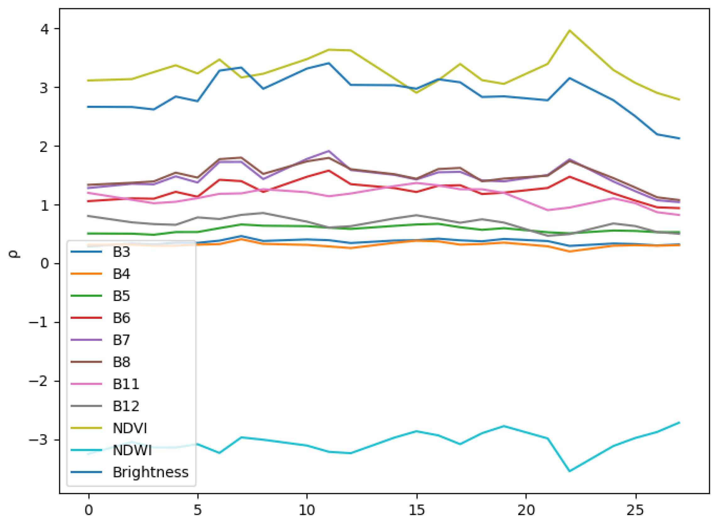
- Spectral resolution defines the bandwidth and the sampling rate used to capture data. A high value for the spectral resolution means more narrow bands pertaining to small parts of the spectrum, and conversely, a low value means broader bands related to large parts of the spectrum. Spectral bands are groups of wavelengths, such as ultraviolet, visible, near-infrared, infrared, and microwave. Based on these, image sensors can be multi-spectral if they are able to cover tens of bands (e.g., Sentinel-2, which collects 12 bands) and hyper-spectral if they can collect thousands, such as Hyperion (part of the EO-1 satellite), which covers 220 spectral bands (0.4–2.5 m) [18].
- Spatial resolution defines the size of the area on the Earth’s surface represented by each pixel from an image. Spatial resolution relates to the level of detail captured in the image, with high resolutions (small pixel size) capturing more and low resolutions (large pixel size) capturing fewer details in an image. For example, most bands observed by the Moderate Resolution Imaging Spectroradiometer (MODIS) have a spatial resolution of 1 km, where each pixel represents a 1 km × 1 km area on the ground [19]. In contrast, images captured from UAVs or drones can have a very small spatial resolution of less than 1 cm [20].
- Radiometric resolution defines the number of discrete signals of given strengths that the sensor can record (also known as dynamic range). A large value of the dynamic range means that more details can be discerned in the recording, e.g., Landsat 7 records 8-bit images and can thus detect 256 unique gray values of the reflected energy [21]; similarly, Sentinel-2 has a 12-bit radiometric resolution (4095 gray values) [22]. In other words, a higher radiometric resolution allows for simultaneous observation of high and low-contrast objects in the scene. For example, a radiometric resolution is necessary to distinguish between subtle differences in ocean color when assessing water quality.
- Temporal resolution defines the frequency at which a given satellite revisits a given observation area. Polar-orbiting satellites have a temporal resolution that can vary from 1 day to 16 days (e.g., for Sentinel-2, this is ten days [22]). The temporal aspects of remote sensing are essential in monitoring and detecting changes in given observation areas (incl. land use change, mowing, and deforestation).
2. Materials and Methods
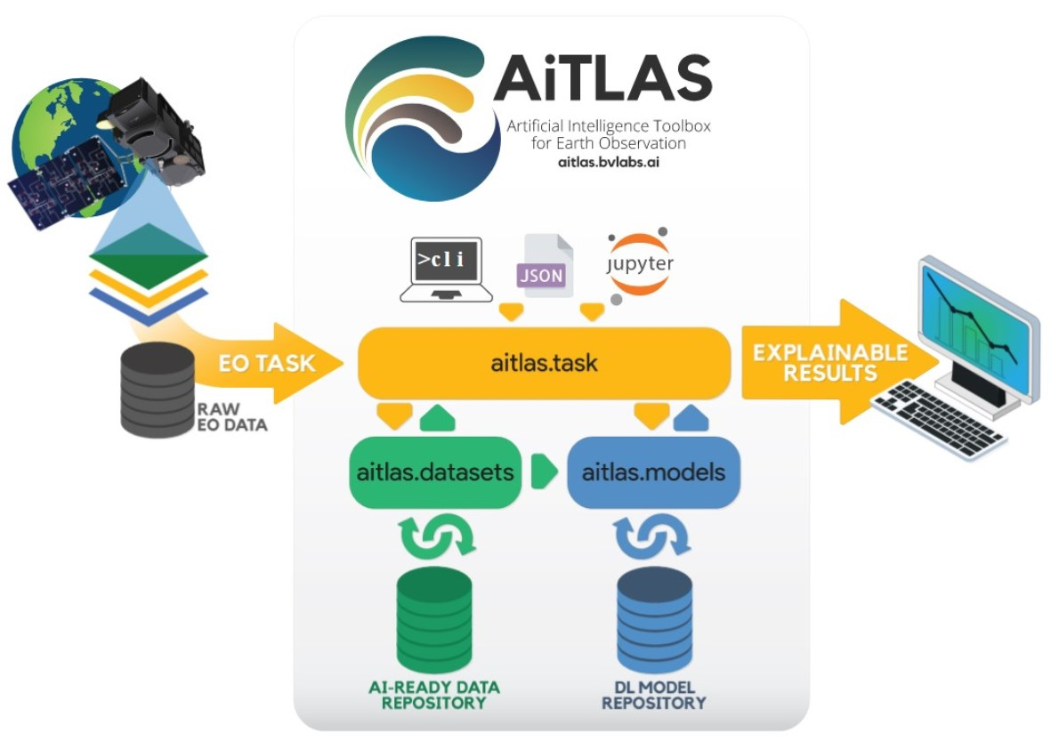
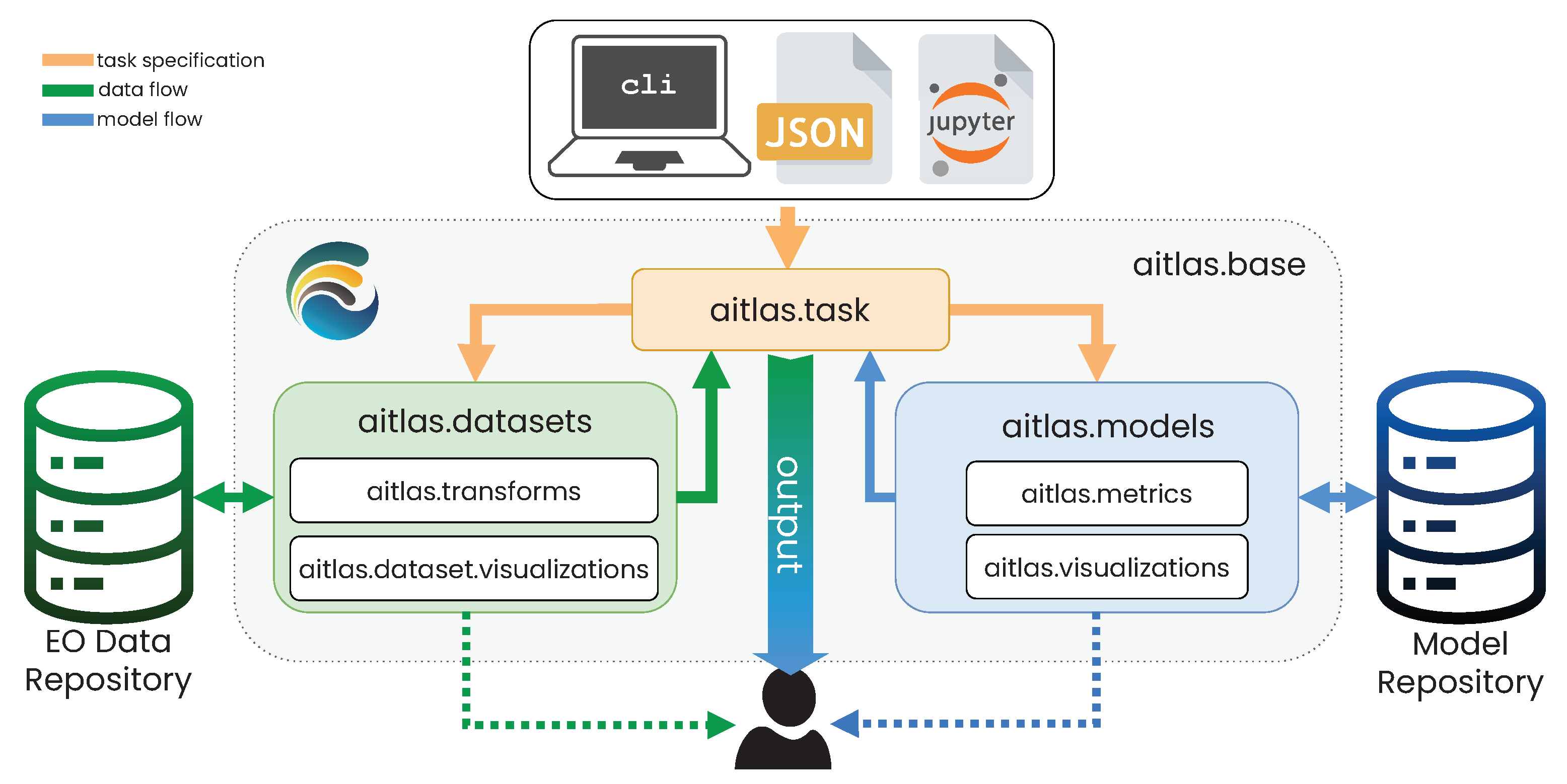
2.1. Design and Implementation of the AiTLAS Toolbox
2.2. EO Data and Common Tasks
2.2.1. Image Scene Classification Tasks

| Name | Image Type | #Images | Image Size | Spatial Resolution | #Labels | Predefined Splits | Image Format |
|---|---|---|---|---|---|---|---|
| UC Merced [33] | Aerial RGB | 2100 | 256 × 256 | 0.3 m | 21 | No | tif |
| WHU-RS19 [34] | Aerial RGB | 1005 | 600 × 600 | 0.5 m | 19 | No | jpg |
| AID [35] | Aerial RGB | 10,000 | 600 × 600 | 0.5 m–8 m | 30 | No | jpg |
| Eurosat [36] | Sat. Multispectral | 27,000 | 64 × 64 | 10 m | 10 | No | jpg/tif |
| PatternNet [37] | Aerial RGB | 30,400 | 256 × 256 | 0.06 m–4.69 m | 38 | No | jpg |
| Resisc45 [4] | Aerial RGB | 31,500 | 256 × 256 | 0.2 m–30 m | 45 | No | jpg |
| RSI-CB256 [38] | Aerial RGB | 24,747 | 256 × 256 | 0.3–3 m | 35 | No | tif |
| RSSCN7 [39] | Aerial RGB | 2800 | 400 × 400 | n/a | 7 | No | jpg |
| SAT6 [40] | RGB + NIR | 405,000 | 28 × 28 | 1 m | 6 | Yes | mat |
| Siri-Whu [41] | Aerial RGB | 2400 | 200 × 200 | 2 m | 12 | No | tif |
| CLRS [42] | Aerial RGB | 15,000 | 256 × 256 | 0.26 m–8.85 m | 25 | No | tif |
| RSD46-WHU [43] | Aerial RGB | 116,893 | 256 × 256 | 0.5 m–2 m | 46 | Yes | jpg |
| Optimal 31 [44] | Aerial RGB | 1860 | 256 × 256 | n/a | 31 | No | jpg |
| Brazilian Coffee Scenes (BSC) [45] | Aerial RGB | 2876 | 64 × 64 | 10 m | 2 | No | jpg |
| SO2Sat [46] | Sat. Multispectral | 400,673 | 32 × 32 | 10 m | 17 | Yes | h5 |
| Name | Image Type | #Images | Image Size | Spatial Resolution | #Labels | #Labels per Image | Predefined Splits | Image Format |
|---|---|---|---|---|---|---|---|---|
| UC Merced (mlc) [31] | Aerial RGB | 2100 | 256 × 256 | 0.3 m | 17 | 3.3 | No | tif |
| MLRSNet [47] | Aerial RGB | 109,161 | 256 × 256 | 0.1 m–10 m | 60 | 5.0 | No | jpg |
| DFC15 [48] | Aerial RGB | 3342 | 600 × 600 | 0.05 m | 8 | 2.8 | Yes | png |
| 20 × 20 | 60 m | |||||||
| 60 × 60 | 20 m | |||||||
| BigEarthNet 19 [13] | Sat. Multispectral | 519,284 | 120 × 120 | 10 m | 19 | 2.9 | Yes | tif, json |
| 20 × 20 | 60 m | |||||||
| 60 × 60 | 20 m | |||||||
| BigEarthNet 43 [49] | Sat. Multispectral | 519,284 | 120 × 120 | 10 m | 43 | 3.0 | Yes | tif, json |
| AID (mlc) [50] | Aerial RGB | 3000 | 600 × 600 | 0.5 m–8 m | 17 | 5.2 | Yes | jpg |
| PlanetUAS [51] | Aerial RGB | 40,479 | 256 × 256 | 3 m | 17 | 2.9 | No | jpg/tiff |
2.2.2. Object Detection Tasks
| Name | Image Type | #Images | #Instances | #Labels | Image Width | Spatial Resolution | Image Format |
|---|---|---|---|---|---|---|---|
| HRRSD [52] | Aerial RGB | 21,761 | 55,740 | 13 | 152–10,569 | 0.15–1.2 m | jpeg |
| DIOR [54] | Aerial RGB | 23,463 | 192,472 | 20 | 800 | 0.5–30 m | jpeg |
| NWPU VHR-10 [55] | Aerial RGB | 800 | 3651 | 10 | ∼800 | 0.08–2 m | jpeg |
| SIMD [56] | Aerial RGB | 5000 | 45,096 | 15 | 1024 | 0.15–0.35 m | jpeg |
2.2.3. Image Semantic Segmentation Tasks
| Name | Image Type | #Images | Image Size | Spatial Resolution | #Labels | Image Format |
|---|---|---|---|---|---|---|
| 4200 × 4700 | ||||||
| LandCover.ai [58] | Aerial RGB | 41 | 9000 × 9500 | 0.25–0.5 m | 5 | geo tif |
| Inria [59] | Aerial RGB | 360 | 5000 × 5000 | 0.3 m | 2 | tif |
| AIRS [60] | Aerial RGB | 1047 | 10,000 × 10,000 | 0.075 m | 2 | tif |
| Amazon Rainforest [61] | Aerial RGB | 60 | 512 × 512 | n/a | 2 | geo tif |
| Chactun [62] | Sat. Multispectral | 2093 | 480 × 480 | 10 m | 3 | geo tiff |
| Massachusetts Roads [57] | Aerial RGB | 1171 | 1500 × 1500 | 1 m | 2 | tiff |
| Massachusetts Buildings [57] | Aerial RGB | 151 | 1500 × 1500 | 1 m | 2 | tiff |
2.2.4. Crop Type Prediction Tasks
2.3. Model Architectures
| Model | Supported Tasks | Based on | |||
|---|---|---|---|---|---|
| Im. Scene Class. | Seman. Segm. | Obj. Detection | Crop Type Pred. | ||
| AlexNet [65] | ✓ | [66] | |||
| CNN-RNN [67] | ✓ | [67] | |||
| ConvNeXt [68] | ✓ | [66] | |||
| DenseNet161 [69] | ✓ | [66] | |||
| EfficientNet [70] | ✓ | [66] | |||
| MLPMixer [71] | ✓ | [72] | |||
| ResNet152 [73] | ✓ | [66] | |||
| ResNet50 [73] | ✓ | [66] | |||
| Swin Transformer [74] | ✓ | [66] | |||
| VGG16 [75] | ✓ | [66] | |||
| Vision Transformer [76] | ✓ | [72] | |||
| DeepLabV3 [77] | ✓ | [66] | |||
| DeepLabV3+ [78] | ✓ | [79] | |||
| FCN [80] | ✓ | [66] | |||
| HRNet [81] | ✓ | [72] | |||
| UNet [82] | ✓ | [79] | |||
| RetinaNet [83] | ✓ | [66] | |||
| Faster R-CNN [84] | ✓ | [66] | |||
| InceptionTime [85] | ✓ | [86] | |||
| LSTM [87] | ✓ | [86] | |||
| MSResNet [88] | ✓ | [86] | |||
| OmniScaleCNN [89] | ✓ | [86] | |||
| StarRNN [90] | ✓ | [86] | |||
| TempCNN [91] | ✓ | [86] | |||
| Transformer for time series classification [92] | ✓ | [86] | |||
3. Results and Discussion: Demonstrating the Potential of AiTLAS
3.1. Image Classification
3.1.1. Data Understanding and Preparation
| Listing 1. Loading an MCC dataset for remote sensing image scene classification using the MultiClassClassificationDataset class from the AiTLAS toolbox. |
 |
| Listing 2. Adding a new MCC dataset in the AiTLAS toolbox. |
 |
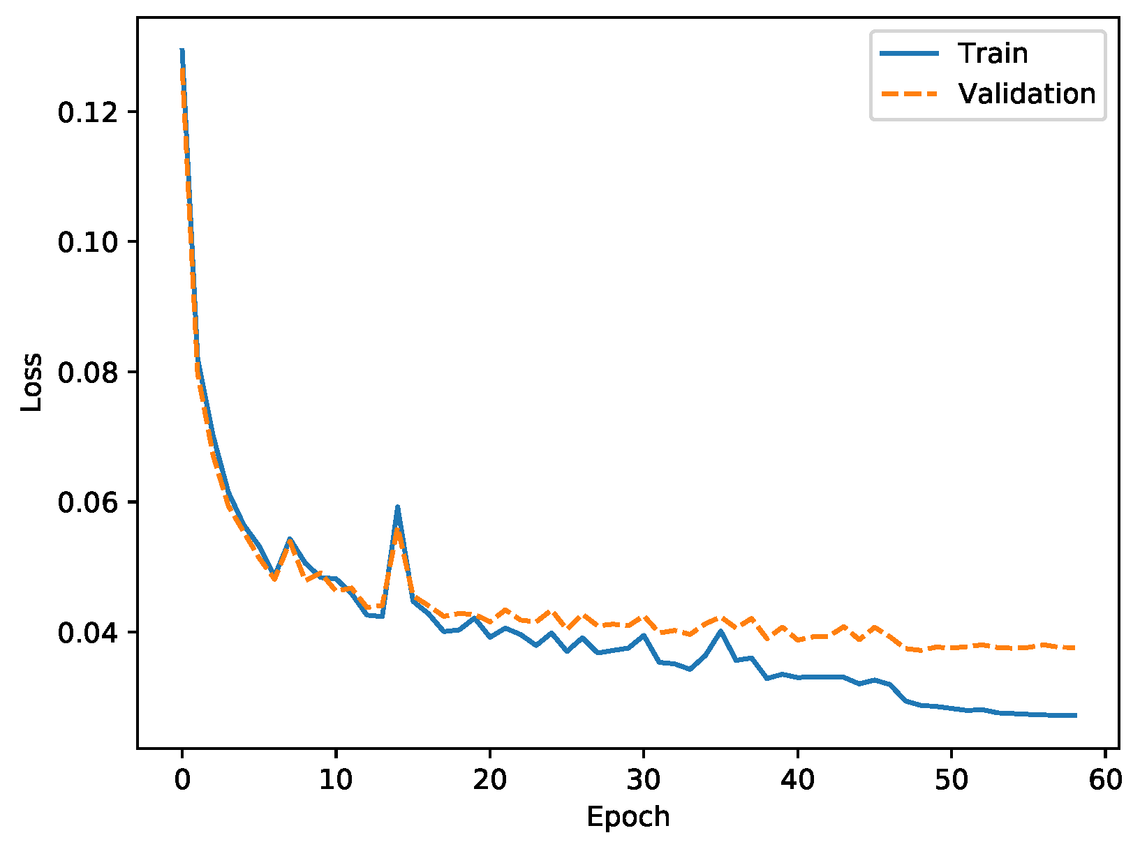
3.1.2. Definition, Execution, and Analysis of a Machine Learning Pipeline
| Listing 3. Creating a model and executing model training. |
 |
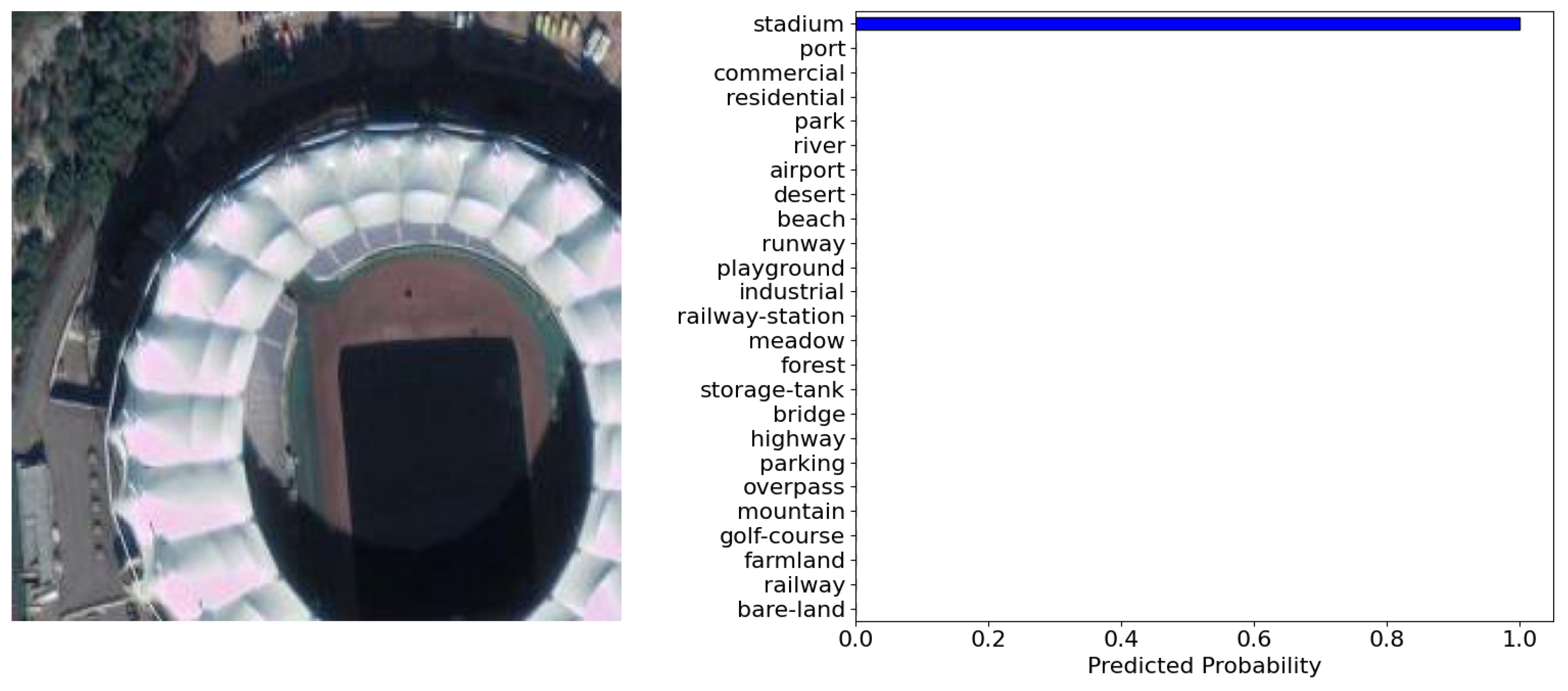
| Listing 4. Evaluating a trained model using images from the test split. |
 |
3.2. Semantic Segmentation
3.2.1. Data Understanding and Preparation
| Listing 5. Adding a new dataset for semantic segmentation in the AiTLAS toolbox. |
 |
3.2.2. Definition, Execution and Analysis of a Machine Learning Pipeline
| Listing 6. Creating an instance of a DeepLabv3 model and executing model training. |
 |
| Listing 7. Evaluating a trained DeepLabv3 model using images from the test split. |
 |
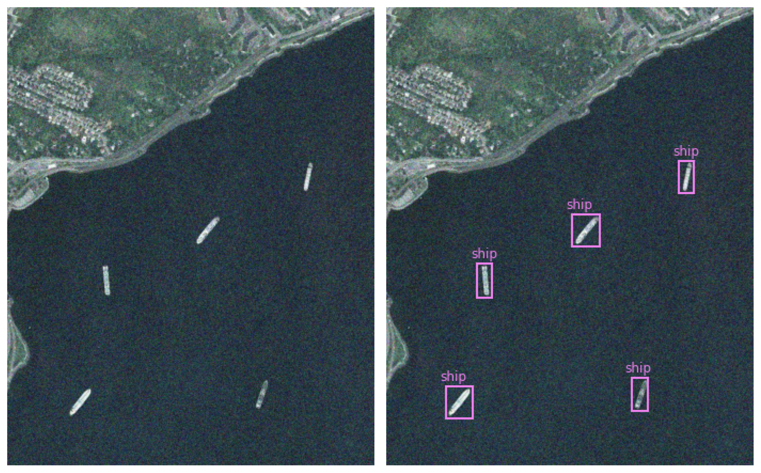
3.3. Object Detection
3.3.1. Data Understanding and Preparation
| Listing 8. Loading HRRSD dataset using the class ObjectDetectionPascalDataset from the AiTLAS toolbox. |
 |
3.3.2. Definition, Execution and Analysis of a Machine Learning Pipeline
| Listing 9. Creating an instance of a Faster R-CNN model and executing model training. |
 |
| Listing 10. Testing a trained model with images from the test split. |
 |
3.4. Crop Type Prediction
3.4.1. Data Understanding and Preparation
| Listing 11. Loading the AiTLAS NLD dataset. |
 |
3.4.2. Definition and Execution of Machine Learning Tasks
| Listing 12. Creating an instance of an LSTM model and executing model training. |
 |
| Listing 13. Evaluating a trained LSTM model. |
 |
3.5. Adding a New Machine Learning Model in AiTLAS
| Listing 14. Adding EfficientNetV2 as a new model for remote sensing image scene classification in the AiTLAS toolbox. |
 |
4. Conclusions
- User-friendly, accessible, and interoperable resources for data analysis through easily configurable and readily usable pipelines. The resources can be easily adapted by adjusting the configuration (JSON) files to a specific task at hand.
- Standardized, verifiable, and reusable data handling, wrangling, and pre-processing approaches for constructing AI-ready data. The AiTLAS datasets are readily available for use through the toolbox and accessible through its EO data catalog (http://eodata.bvlabs.ai), which incorporates FAIR [124] ontology-based semantic (meta) data descriptions of AI-ready datasets;
- Modular and configurable modeling approaches and (pre-trained) models. The implemented approaches can be easily adjusted to different setups and novel analysis pipelines. Moreover, AiTLAS includes the most extensive open-source catalog of pre-trained EO deep-learning models (currently with more than 500 models) that have been pre-trained on a variety of different datasets and are readily available for practical applications.
- Standardized and reproducible benchmark protocols (for data and models) that are essential for developing trustworthy, reproducible, and reusable resources. AiTLAS provides the resources and the necessary mechanisms for reconciling these protocols across tasks, models (and model configurations), and processing details of the datasets being used.
Author Contributions
Funding
Data Availability Statement
Acknowledgments
Conflicts of Interest
Appendix A. Third-Party Dependencies
| Library | Scope of Usage | Purpose |
|---|---|---|
| PyTorch Vision [66] | aitlas.models | Pre-built deep-learning model architectures. |
| PyTorch Image Models [72] | aitlas.models | Pre-built deep-learning model architectures. |
| Segmentation Models PyTorch [79] | aitlas.models | Pre-built deep-learning model architectures specifically for segmentation tasks. |
| Albumentations [129] | aitlas.transforms | Applying transormations and augmentations. |
| NumPy [130] | aitlas.base | General scientific computing |
| Scikit-learn [131] | aitlas.base | Used for metric calculations |
| Scikit-multilearn [132] | aitlas.tasks | Used for stratified dataset splitting. |
| Seaborn [133] | aitlas.visualizations | For visualizations. |
| Matplotlib [133] | aitlas.visualizations | For visualizations |
| TensorBoard [27] | aitlas.base | Enable logging the train/validation loss during model training as well as any other supported metrics. This then allows for those statistics to be visualized in the TensorBoard UI. |
| zipp [134] | aitlas.utils | Enables working with zip files. |
| dill [135] | aitlas.utils | Extends Python’s pickle module for serializing and de-serializing Python objects to the majority of the built-in data types. |
| lmdb [136] | aitlas.datasets | Enables working with LMDB data. |
| tifffile [137] | aitlas.utils | Reads TIFF files from any storage. |
| h5py [138] | aitlas.datasets | Provides an interface to the HDF5 binary data format. |
| click [139] | aitlas.base | Enables creating command line interfaces. |
| munch [140] | aitlas.base | Provides attribute-style access to objects. |
| marshmallow [141] | aitlas.base | It is an ORM/ODM/framework-agnostic library for converting complex data types to and from native Python data types. |
| Pytoch Metrics [142] | aitlas.metrics | Utility library used for computing performance metrics. |
Appendix B. Split Task within the AiTLAS Toolbox for Creating Train, Validation and Test Splits
| Listing A1. Configuration file for creating train, validation and test splits. |
 |
| Listing A2. Example csv file with the required format by the AiTLAS toolbox for remote sensing image scene classification datasets. |
 |
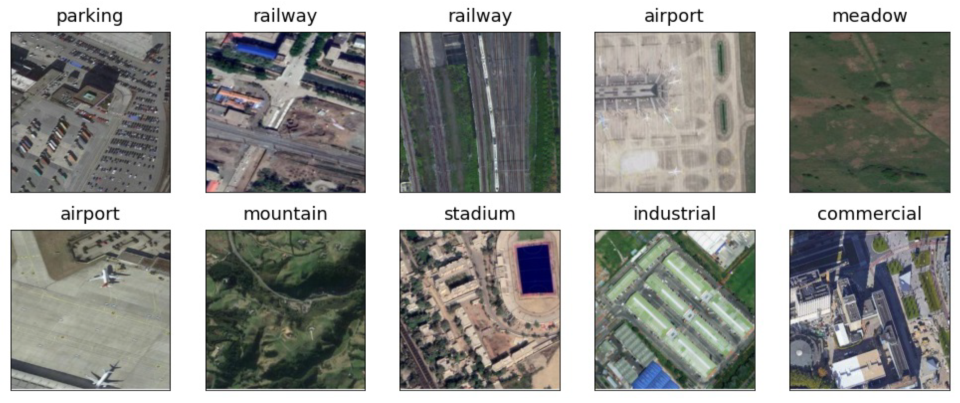
Appendix C. Remote Sensing Image Scene Classification
| Listing A3. Load a dataset using the AiTLAS toolbox, inspect images and calculate the class distribution. |
 |

| Listing A4. Load the training and validation dataset. |
 |
| Listing A5. Creating a model and start of model training. |
 |
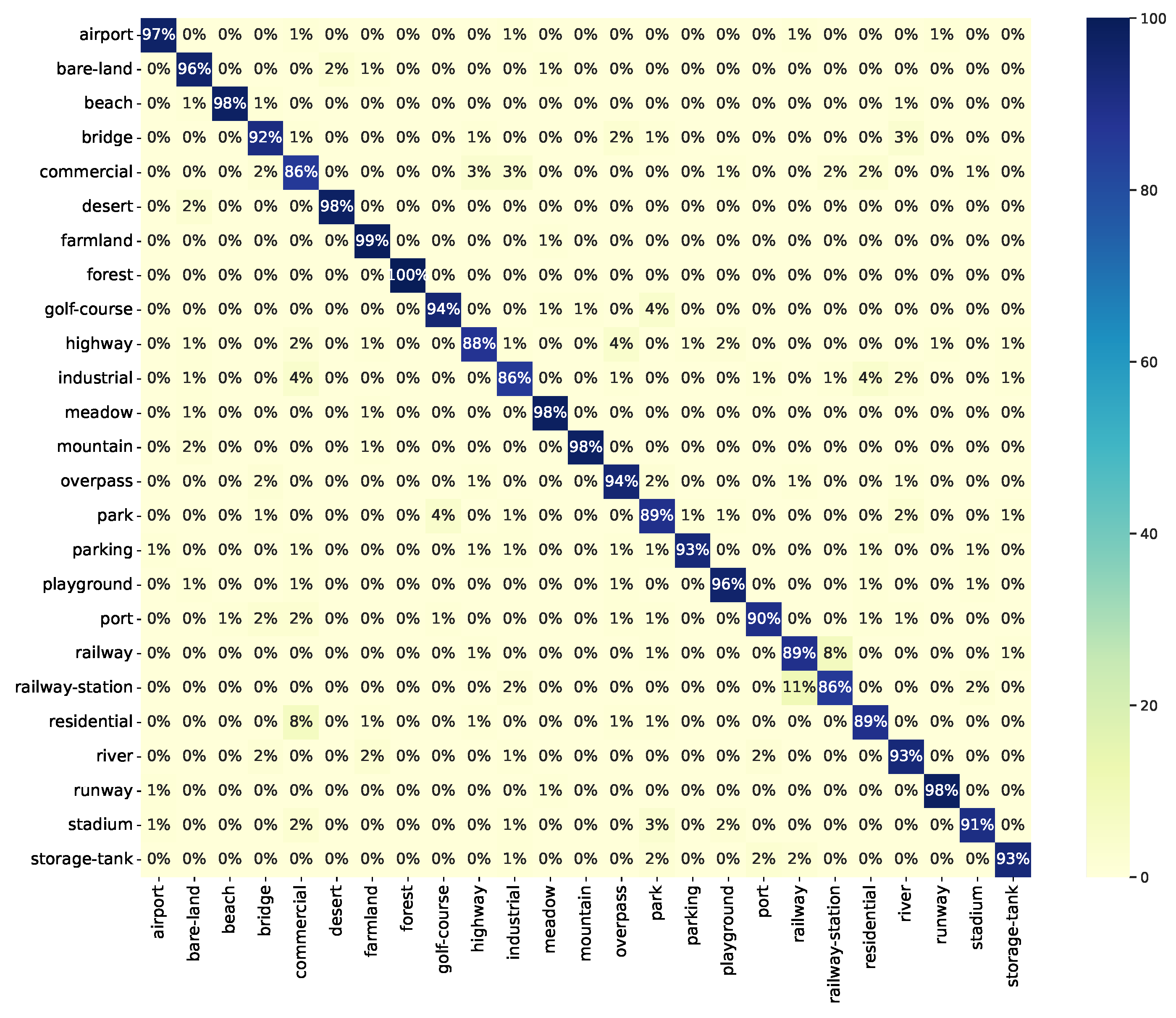
| Listing A6. Testing the model using the images from the test split. |
 |
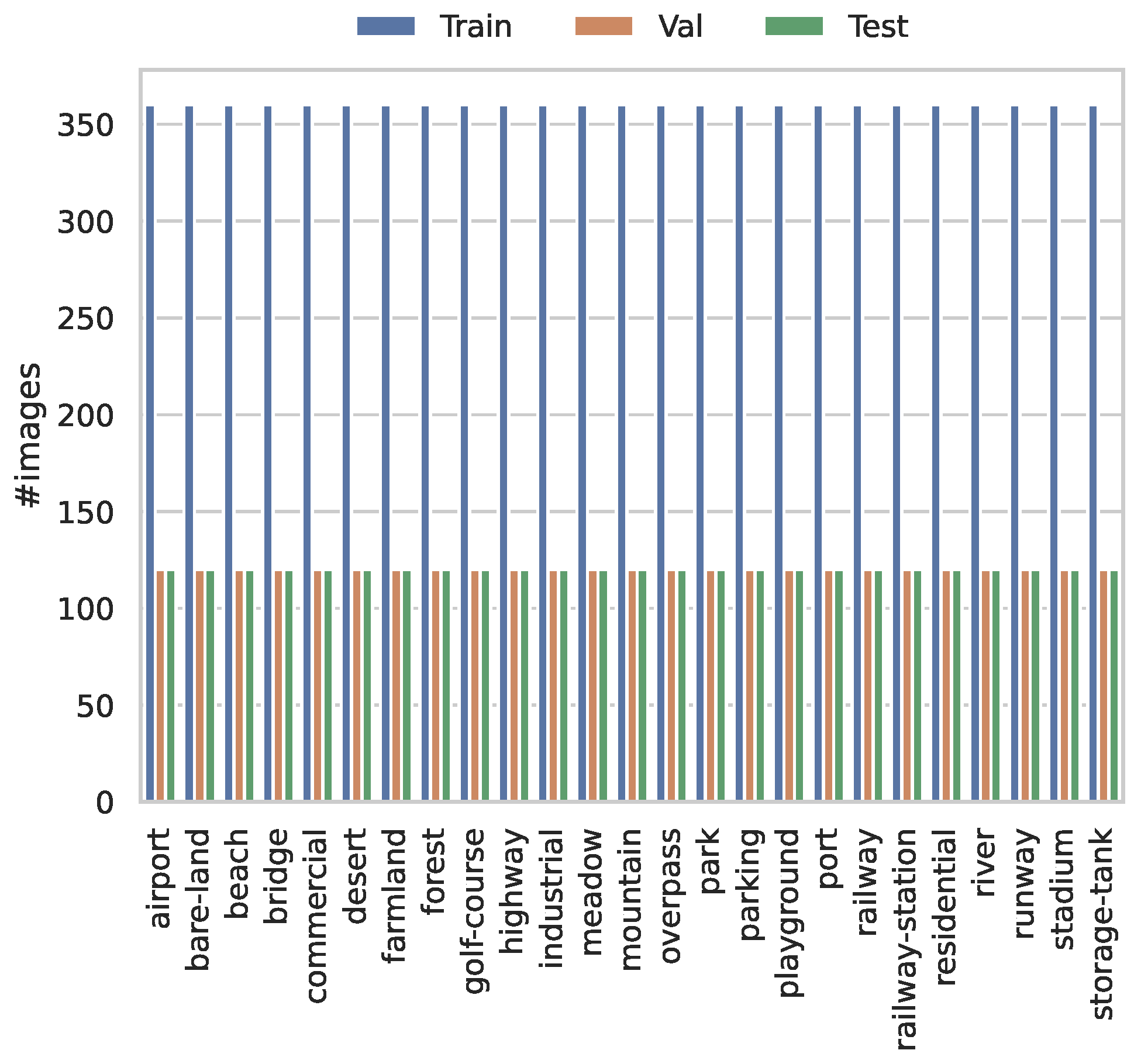
| Model/Metric | Accuracy | Macro Precision | Weighted Precision | Macro Recall | Weighted Recall | Macro F1 score | Weighted F1 Score | Avg. Time/Epoch (s) | Total Time (s) | Best Epoch |
|---|---|---|---|---|---|---|---|---|---|---|
| Trained from scratch | 65.47 | 66.41 | 66.41 | 65.47 | 65.47 | 65.49 | 65.49 | 24.96 | 1173 | 32 |
| Pre-trained on ImageNet-1K | 93.20 | 93.29 | 93.29 | 93.20 | 93.20 | 93.22 | 93.22 | 25.32 | 785 | 21 |
| Label | Precision | Recall | F1 Score |
|---|---|---|---|
| airport | 97.48 | 96.67 | 97.07 |
| bare-land | 92.00 | 95.83 | 93.88 |
| beach | 99.15 | 97.50 | 98.32 |
| bridge | 90.91 | 91.67 | 91.29 |
| commercial | 79.84 | 85.83 | 82.73 |
| desert | 97.50 | 97.50 | 97.50 |
| farmland | 93.70 | 99.17 | 96.36 |
| forest | 100.00 | 100.00 | 100.00 |
| golf-course | 94.96 | 94.17 | 94.56 |
| highway | 92.11 | 87.50 | 89.74 |
| industrial | 88.79 | 85.83 | 87.29 |
| meadow | 96.72 | 98.33 | 97.52 |
| mountain | 99.15 | 97.50 | 98.32 |
| overpass | 89.68 | 94.17 | 91.87 |
| park | 85.60 | 89.17 | 87.35 |
| parking | 98.25 | 93.33 | 95.73 |
| playground | 95.04 | 95.83 | 95.44 |
| port | 94.74 | 90.00 | 92.31 |
| railway | 86.29 | 89.17 | 87.70 |
| railway-station | 88.79 | 85.83 | 87.29 |
| residential | 90.68 | 89.17 | 89.92 |
| river | 90.32 | 93.33 | 91.80 |
| runway | 98.33 | 98.33 | 98.33 |
| stadium | 95.61 | 90.83 | 93.16 |
| storage-tank | 96.55 | 93.33 | 94.92 |

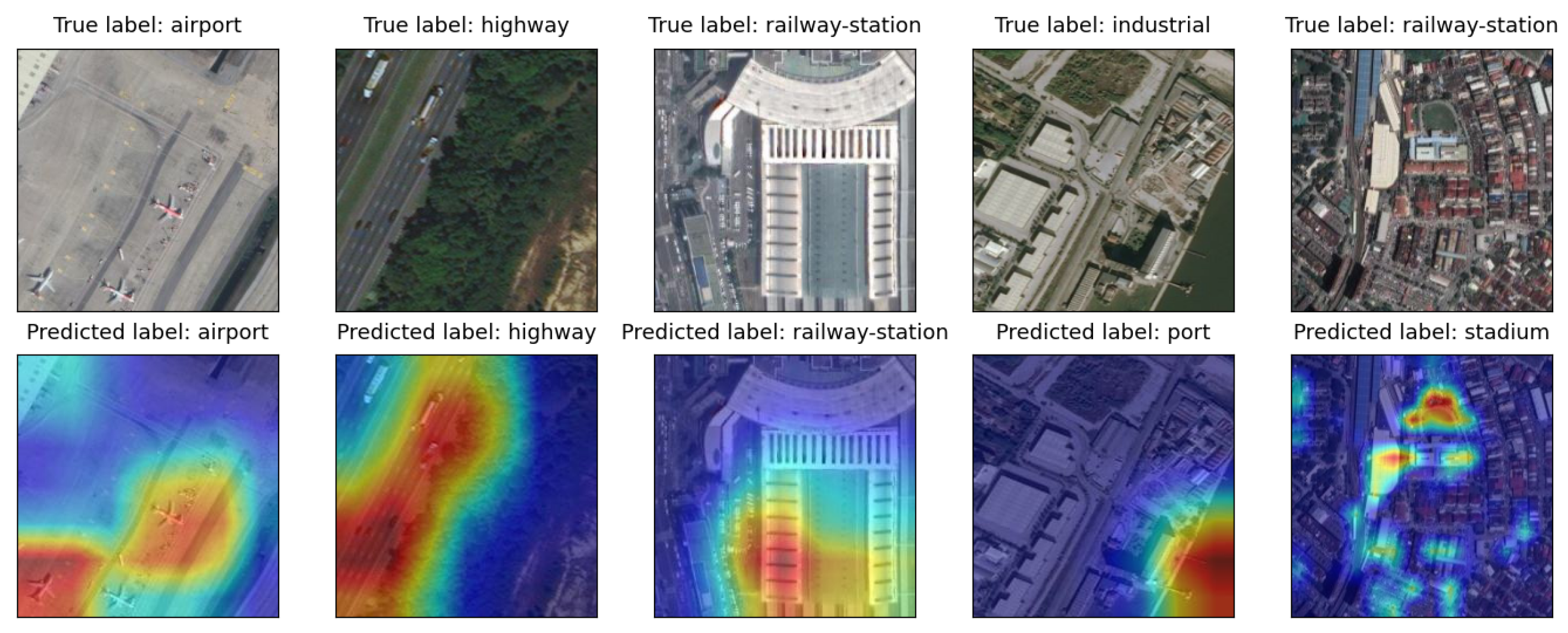
| Listing A7. Getting predictions for images from external source. |
 |
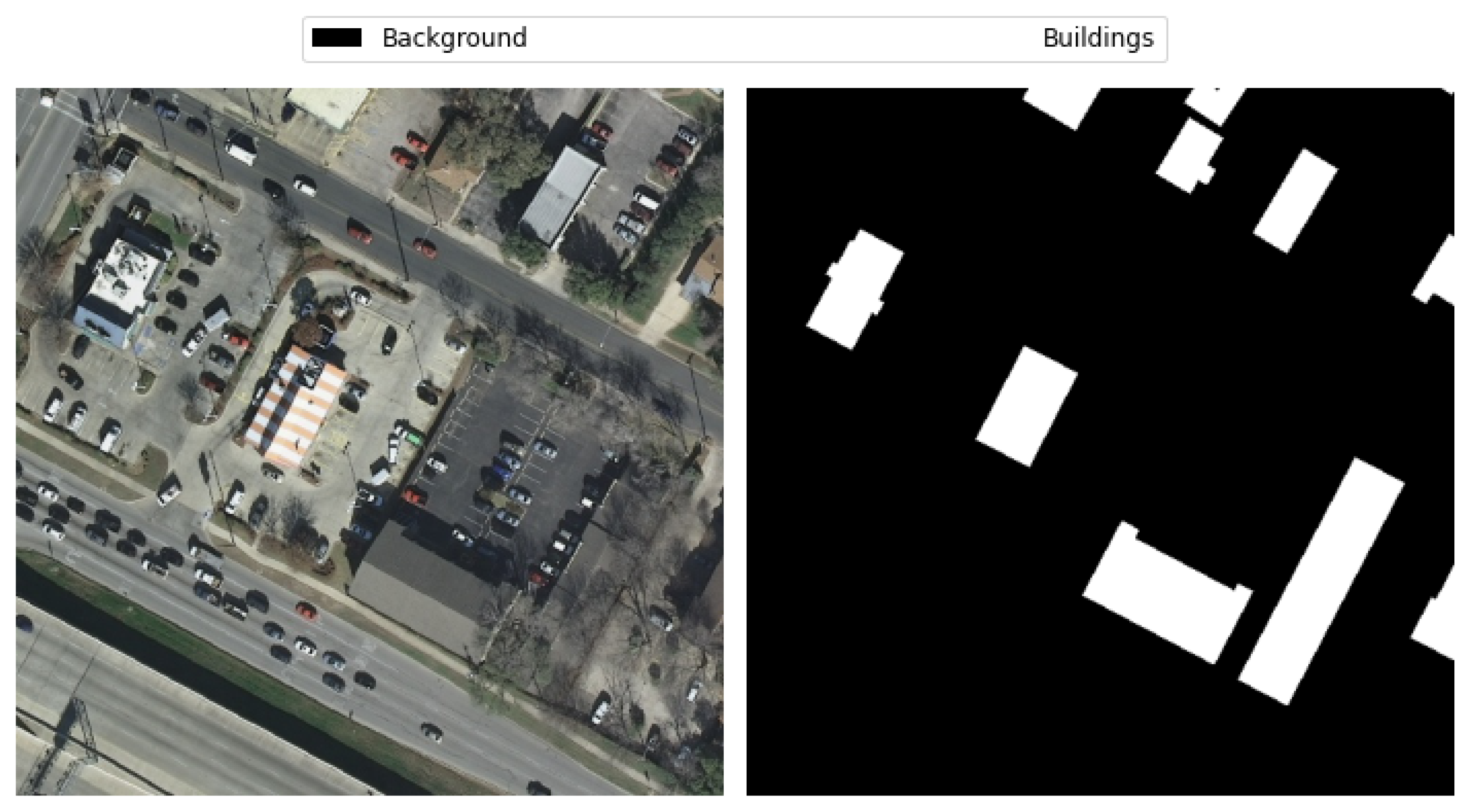
Appendix D. Semantic Segmentation of Remote Sensing Images
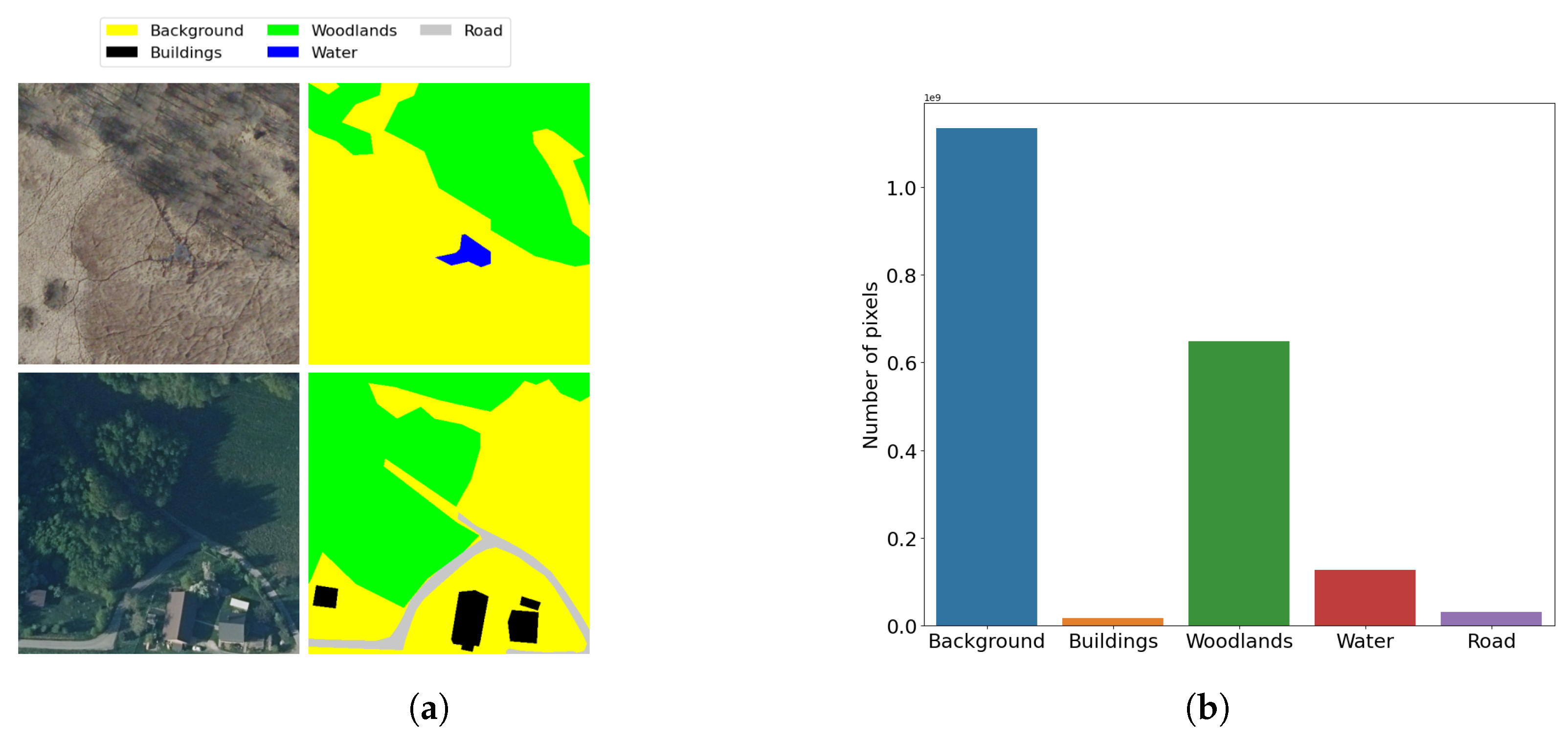
| Listing A8. Load the LandCoverAiDataset dataset from the AiTLAS toolbox, inspect images and masks, and calculate the pixel distribution across the labels. |
 |
| Listing A9. Load the training and validation dataset for semantic segmentation. |
 |
| Listing A10. Creating a DeepLabv3 model and starting the training. |
 |

| Listing A11. Testing the model using the images from the test split. |
 |
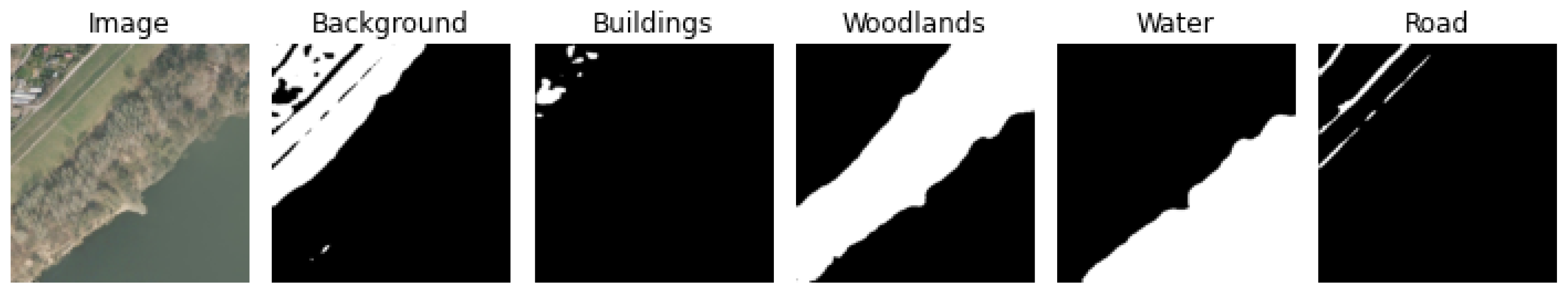
| Model/Label | Background | Buildings | Woodlands | Water | Road | mIoU | Avg. Time/Epoch (s) | Total Time (s) | Best Epoch |
|---|---|---|---|---|---|---|---|---|---|
| Trained from scratch | 93.813 | 80.304 | 91.952 | 94.877 | 69.190 | 86.027 | 299.241 | 16159 | 44 |
| Pre-trained on COCO | 93.857 | 80.650 | 91.964 | 95.145 | 68.846 | 86.093 | 300.58 | 17734 | 49 |
| Listing A12. Getting predictions for images from external source. |
 |

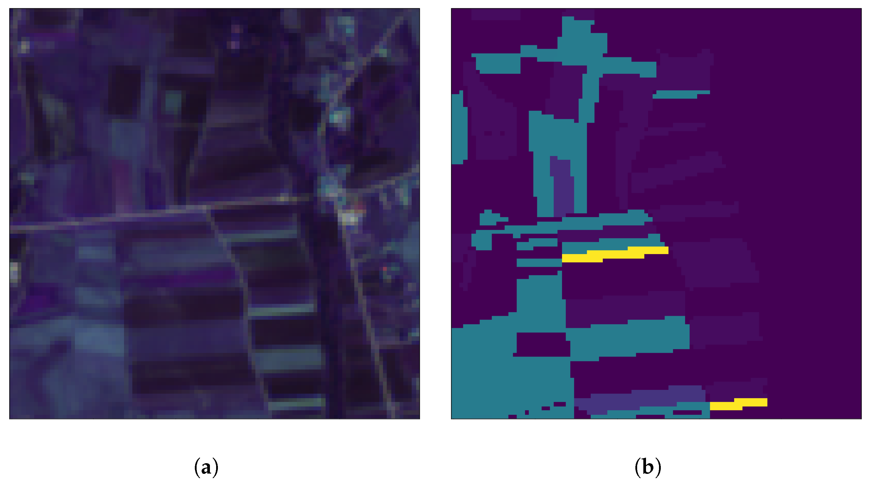
Appendix E. Remote Sensing Image Object Detection
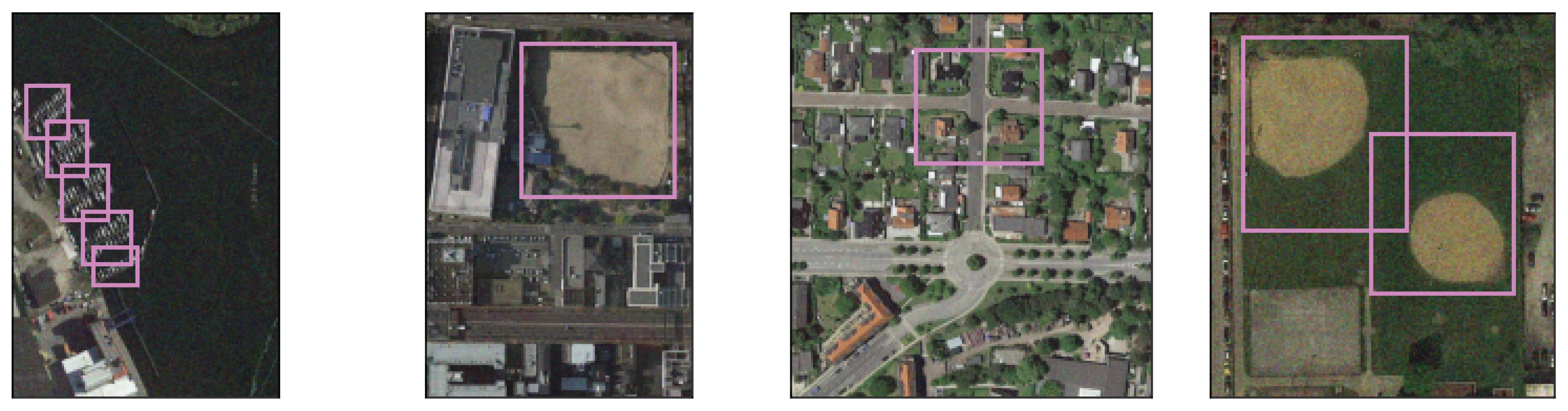
| Listing A13. Load a dataset using the AiTLAS toolbox, inspect images and calculate the number of object instances for each category/label. |
 |
| Listing A14. Load the training and validation dataset. |
 |
| Listing A15. Creating a Faster R-CNN model and start of model training. |
 |
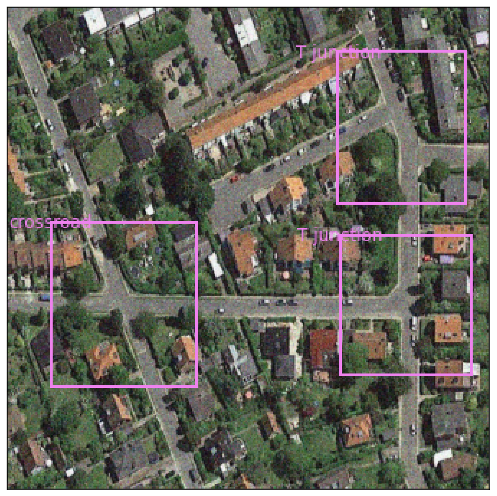
| Label | Faster R-CNN (Pretrained) | Faster R-CNN |
|---|---|---|
| Airplane | 96.86 | 94.71 |
| Baseball Diamond | 79.75 | 80.13 |
| Basketball Court | 59.25 | 44.96 |
| Bridge | 82.22 | 78.55 |
| Crossroad | 77.06 | 71.78 |
| Ground Track Field | 95.62 | 92.84 |
| Harbor | 89.00 | 88.61 |
| Parking Lot | 53.80 | 51.22 |
| Ship | 86.61 | 78.50 |
| Storage Tank | 93.56 | 89.67 |
| T Junction | 66.83 | 69.12 |
| Tennis Court | 87.97 | 79.31 |
| Vehicle | 90.14 | 86.96 |
| Mean AP | 81.436 | 77.412 |
| Avg. time / epoch (s) | 221.96 | 244.63 |
| Total time (s) | 5993 | 10030 |
| Best epoch | 17 | 31 |
| Listing A16. Testing the model using the images from the test split. |
 |
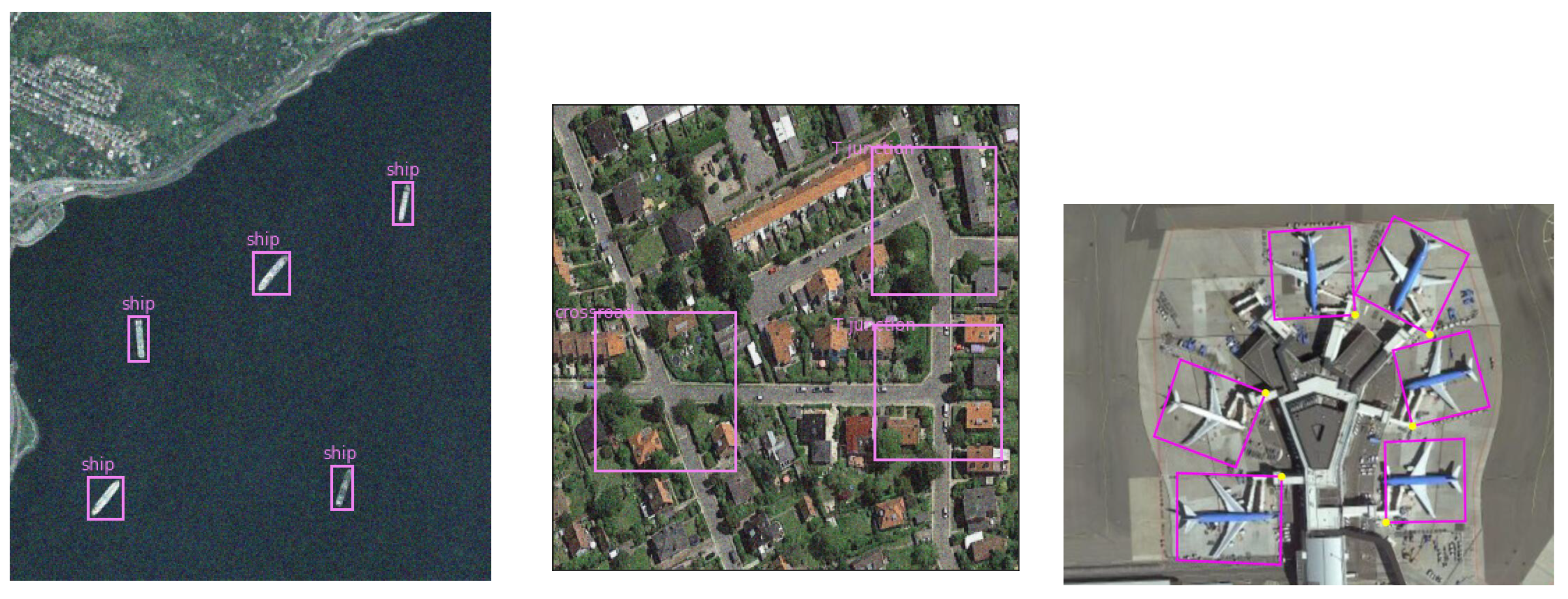
| Listing A17. Getting bounding boxes and labels for images from external source. |
 |

Appendix F. Crop Type Prediction Using Satellite Time Series Data
| Listing A18. Load the dataset. |
 |
| Listing A19. Inspect the dataset. |
 |

| Listing A20. Load train and validation the dataset. |
 |
| Listing A21. Train the model. |
 |

| Listing A22. Test the model. |
 |
| Dataset Year | Accuracy | Weighted F1 Score | Kappa |
|---|---|---|---|
| 2017 | 84.28 | 82.48 | 77.22 |
| 2018 | 84.49 | 84.32 | 78.79 |
| 2019 | 85.25 | 84.10 | 79.55 |
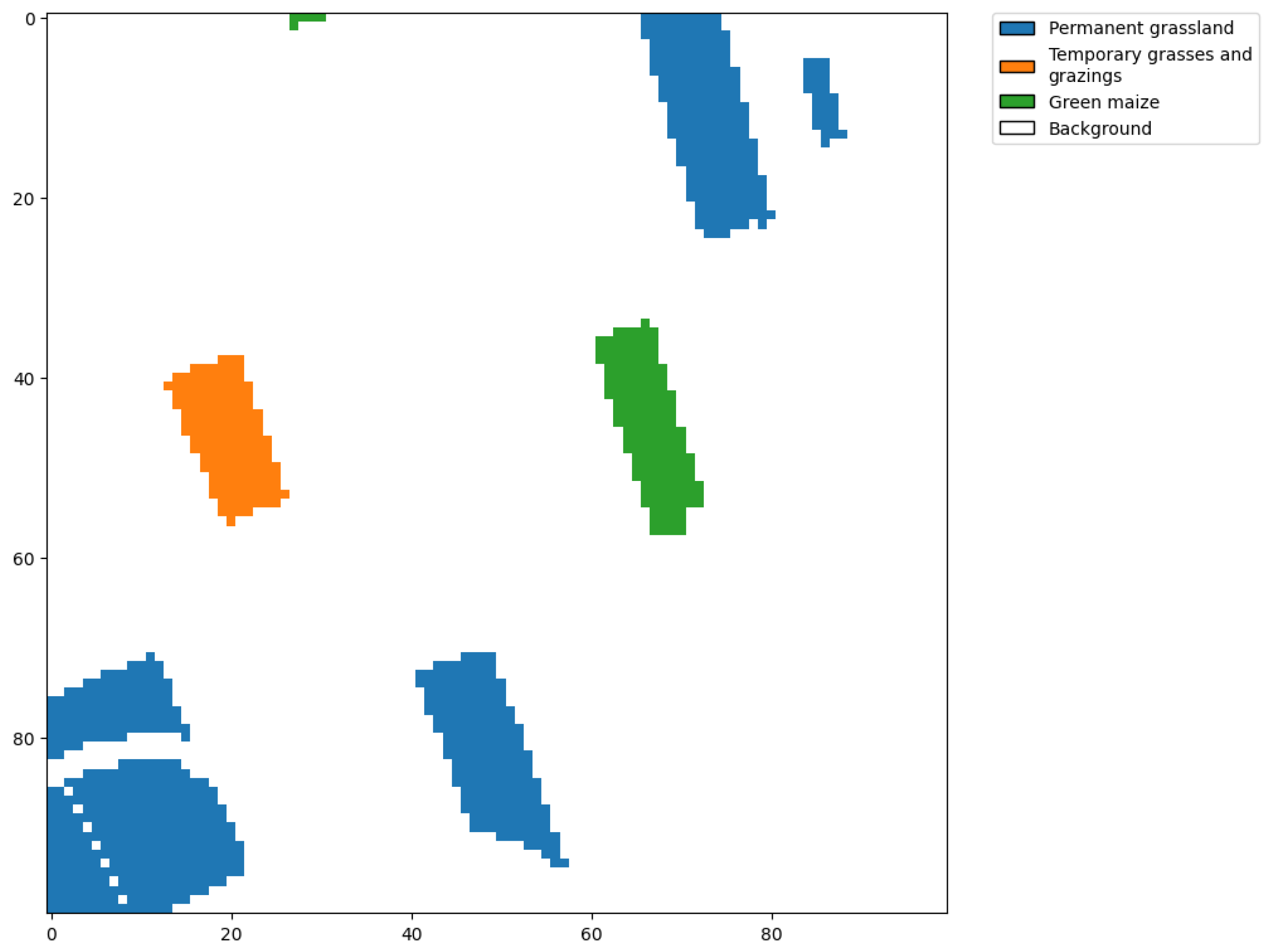
| Crop Type | 2017 | 2018 | 2019 |
|---|---|---|---|
| Permanent grassland | 86.72 | 85.78 | 86.82 |
| Temporary grasses and grazings | 45.23 | 59.34 | 53.66 |
| Green maize | 96.10 | 95.09 | 96.14 |
| Potatoes (including seed potatoes) | 95.37 | 94.84 | 95.45 |
| Common winter wheat and spelt | 94.86 | 95.75 | 96.28 |
| Sugar beet (excluding seed) | 95.62 | 92.36 | 95.28 |
| Other farmland | 62.45 | 61.81 | 60.05 |
| Onions | 89.76 | 93.68 | 92.51 |
| Flowers and ornamental plants (excluding nurseries) | 83.18 | 78.30 | 79.67 |
| Spring barley | 92.30 | 91.12 | 90.80 |
References
- Christopherson, J.; Chandra, S.N.R.; Quanbeck, J.Q. 2019 Joint Agency Commercial Imagery Evaluation—Land Remote Sensing Satellite Compendium; Technical Report; US Geological Survey: Reston, VA, USA, 2019. [Google Scholar]
- Tupin, F.; Inglada, J.; Nicolas, J.M. Remote Sensing Imagery; John Wiley & Sons: Hoboken, NJ, USA, 2014. [Google Scholar]
- Dimitrovski, I.; Kitanovski, I.; Kocev, D.; Simidjievski, N. Current trends in deep learning for Earth Observation: An open-source benchmark arena for image classification. ISPRS J. Photogramm. Remote Sens. 2023, 197, 18–35. [Google Scholar] [CrossRef]
- Cheng, G.; Han, J.; Lu, X. Remote Sensing Image Scene Classification: Benchmark and State of the Art. Proc. IEEE 2017, 105, 1865–1883. [Google Scholar] [CrossRef]
- Tang, L.; Shao, G. Drone remote sensing for forestry research and practices. J. For. Res. 2015, 26, 791–797. [Google Scholar] [CrossRef]
- Roy, P.; Ranganath, B.; Diwakar, P.; Vohra, T.; Bhan, S.; Singh, I.; Pandian, V. Tropical forest typo mapping and monitoring using remote sensing. Remote Sens. 1991, 12, 2205–2225. [Google Scholar] [CrossRef]
- Sunar, F.; Özkan, C. Forest fire analysis with remote sensing data. Int. J. Remote Sens. 2001, 22, 2265–2277. [Google Scholar] [CrossRef]
- Poursanidis, D.; Chrysoulakis, N. Remote Sensing, natural hazards and the contribution of ESA Sentinels missions. Remote Sens. Appl. Soc. Environ. 2017, 6, 25–38. [Google Scholar] [CrossRef]
- Sishodia, R.P.; Ray, R.L.; Singh, S.K. Applications of remote sensing in precision agriculture: A review. Remote Sens. 2020, 12, 3136. [Google Scholar] [CrossRef]
- Cox, H.; Kelly, K.; Yetter, L. Using remote sensing and geospatial technology for climate change education. J. Geosci. Educ. 2014, 62, 609–620. [Google Scholar] [CrossRef]
- Collis, R.T.; Creasey, D.; Grasty, R.; Hartl, P.; deLoor, G.; Russel, P.; Salerno, A.; Schaper, P. Remote Sensing for Environmental Sciences; Springer Science & Business Media: Berlin, Germany, 2012; Volume 18. [Google Scholar]
- Christie, G.; Fendley, N.; Wilson, J.; Mukherjee, R. Functional Map of the World. In Proceedings of the 2018 IEEE/CVF Conference on Computer Vision and Pattern Recognition, Salt Lake City, UT, USA, 18–23 June 2018; pp. 6172–6180. [Google Scholar] [CrossRef]
- Sumbul, G.; de Wall, A.; Kreuziger, T.; Marcelino, F.; Costa, H.; Benevides, P.; Caetano, M.; Demir, B.; Markl, V. BigEarthNet-MM: A Large-Scale, Multimodal, Multilabel Benchmark Archive for Remote Sensing Image Classification and Retrieval [Software and Data Sets]. IEEE Geosci. Remote Sens. Mag. 2021, 9, 174–180. [Google Scholar] [CrossRef]
- Long, Y.; Xia, G.S.; Li, S.; Yang, W.; Yang, M.Y.; Zhu, X.X.; Zhang, L.; Li, D. On Creating Benchmark Dataset for Aerial Image Interpretation: Reviews, Guidances and Million-AID. IEEE J. Sel. Top. Appl. Earth Obs. Remote Sens. 2021, 14, 4205–4230. [Google Scholar] [CrossRef]
- Bastani, F.; Wolters, P.; Gupta, R.; Ferdinando, J.; Kembhavi, A. Satlas: A Large-Scale, Multi-Task Dataset for Remote Sensing Image Understanding. arXiv 2022, arXiv:2211.15660. [Google Scholar] [CrossRef]
- Neupane, B.; Horanont, T.; Aryal, J. Deep Learning-Based Semantic Segmentation of Urban Features in Satellite Images: A Review and Meta-Analysis. Remote Sens. 2021, 13, 808. [Google Scholar] [CrossRef]
- Xia, G.S.; Bai, X.; Ding, J.; Zhu, Z.; Belongie, S.; Luo, J.; Datcu, M.; Pelillo, M.; Zhang, L. DOTA: A Large-Scale Dataset for Object Detection in Aerial Images. In Proceedings of the IEEE Conference on Computer Vision and Pattern Recognition (CVPR), Salt Lake City, UT, USA, 18–23 June 2018. [Google Scholar]
- Pearlman, J.; Barry, P.; Segal, C.; Shepanski, J.; Beiso, D.; Carman, S. Hyperion, a space-based imaging spectrometer. IEEE Trans. Geosci. Remote Sens. 2003, 41, 1160–1173. [Google Scholar] [CrossRef]
- King, M.; Herring, D. SATELLITES | Research (Atmospheric Science). In Encyclopedia of Atmospheric Sciences; Holton, J.R., Ed.; Academic Press: Oxford, UK, 2003; pp. 2038–2047. [Google Scholar] [CrossRef]
- Osco, L.P.; Marcato Junior, J.; Marques Ramos, A.P.; de Castro Jorge, L.A.; Fatholahi, S.N.; de Andrade Silva, J.; Matsubara, E.T.; Pistori, H.; Gonçalves, W.N.; Li, J. A review on deep learning in UAV remote sensing. Int. J. Appl. Earth Obs. Geoinf. 2021, 102, 102456. [Google Scholar] [CrossRef]
- Roy, D.P.; Wulder, M.A.; Loveland, T.R.; Woodcock, C.E.; Allen, R.G.; Anderson, M.C.; Helder, D.; Irons, J.R.; Johnson, D.M.; Kennedy, R.; et al. Landsat-8: Science and product vision for terrestrial global change research. Remote Sens. Environ. 2014, 145, 154–172. [Google Scholar] [CrossRef]
- Drusch, M.; Del Bello, U.; Carlier, S.; Colin, O.; Fernandez, V.; Gascon, F.; Hoersch, B.; Isola, C.; Laberinti, P.; Martimort, P.; et al. Sentinel-2: ESA’s Optical High-Resolution Mission for GMES Operational Services. Remote Sens. Environ. 2012, 120, 25–36. [Google Scholar] [CrossRef]
- Sentinel Hub: Cloud API For Satellite Imagery. 2023. Available online: https://www.sentinel-hub.com/ (accessed on 8 March 2023).
- UP42: Simplified Access to Geospatial Data and Processing. 2023. Available online: https://up42.com/ (accessed on 8 March 2023).
- De Vroey, M.; Radoux, J.; Zavagli, M.; De Vendictis, L.; Heymans, D.; Bontemps, S.; Defourny, P. Performance Assessment of the Sen4CAP Mowing Detection Algorithm on a Large Reference Data Set of Managed Grasslands. In Proceedings of the 2021 IEEE International Geoscience and Remote Sensing Symposium IGARSS, Brussels, Belgium, 11–16 July 2021; pp. 743–746. [Google Scholar] [CrossRef]
- Grizonnet, M.; Michel, J.; Poughon, V.; Inglada, J.; Savinaud, M.; Cresson, R. Orfeo ToolBox: Open source processing of remote sensing images. Open Geospat. Data Softw. Stand. 2017, 2, 15. [Google Scholar] [CrossRef]
- Abadi, M.; Agarwal, A.; Barham, P.; Brevdo, E.; Chen, Z.; Citro, C.; Corrado, G.S.; Davis, A.; Dean, J.; Devin, M.; et al. TensorFlow: Large-Scale Machine Learning on Heterogeneous Systems. arXiv 2015, arXiv:1603.04467. [Google Scholar]
- Rolland, J.F.; Castel, F.; Haugommard, A.; Aubrun, M.; Yao, W.; Dumitru, C.O.; Datcu, M.; Bylicki, M.; Tran, B.H.; Aussenac-Gilles, N.; et al. Candela: A Cloud Platform for Copernicus Earth Observation Data Analytics. In Proceedings of the IGARSS 2020—2020 IEEE International Geoscience and Remote Sensing Symposium, Waikoloa, HI, USA, 26 September–2 October 2020; pp. 3104–3107. [Google Scholar] [CrossRef]
- Stewart, A.J.; Robinson, C.; Corley, I.A.; Ortiz, A.; Lavista Ferres, J.M.; Banerjee, A. TorchGeo: Deep Learning with Geospatial Data. In Proceedings of the SIGSPATIAL ’22: 30th International Conference on Advances in Geographic Information Systems, Seattle, WA, USA, 1–4 November 2022; Association for Computing Machinery: New York, NY, USA; pp. 1–12. [Google Scholar] [CrossRef]
- Paszke, A.; Gross, S.; Massa, F.; Lerer, A.; Bradbury, J.; Chanan, G.; Killeen, T.; Lin, Z.; Gimelshein, N.; Antiga, L.; et al. PyTorch: An Imperative Style, High-Performance Deep Learning Library. In Advances in Neural Information Processing Systems 32; Curran Associates, Inc.: Red Hook, NY, USA, 2019; pp. 8024–8035. [Google Scholar]
- Chaudhuri, B.; Demir, B.; Chaudhuri, S.; Bruzzone, L. Multilabel Remote Sensing Image Retrieval Using a Semisupervised Graph-Theoretic Method. IEEE Trans. Geosci. Remote Sens. 2018, 56, 1144–1158. [Google Scholar] [CrossRef]
- Tsoumakas, G.; Katakis, I. Multi-Label Classification: An Overview. Int. J. Data Warehous. Min. 2009, 3, 1–13. [Google Scholar] [CrossRef]
- Yang, Y.; Newsam, S. Bag-of-Visual-Words and Spatial Extensions for Land-Use Classification. In Proceedings of the GIS ’10: 18th SIGSPATIAL International Conference on Advances in Geographic Information Systems, San Jose, CA, USA, 2–5 November 2010; Association for Computing Machinery: New York, NY, USA; pp. 270–279. [Google Scholar]
- Xia, G.S.; Yang, W.; Delon, J.; Gousseau, Y.; Sun, H.; Maître, H. Structural High-resolution Satellite Image Indexing. Int. Arch. Photogramm. Remote Sens. Spat. Inf. Sci. ISPRS Arch. 2010, 38, 1–6. [Google Scholar]
- Xia, G.S.; Hu, J.; Hu, F.; Shi, B.; Bai, X.; Zhong, Y.; Zhang, L.; Lu, X. AID: A Benchmark Data Set for Performance Evaluation of Aerial Scene Classification. IEEE Trans. Geosci. Remote Sens. 2017, 55, 3965–3981. [Google Scholar] [CrossRef]
- Helber, P.; Bischke, B.; Dengel, A.; Borth, D. Eurosat: A novel dataset and deep learning benchmark for land use and land cover classification. IEEE J. Sel. Top. Appl. Earth Obs. Remote Sens. 2019, 12, 2217–2226. [Google Scholar] [CrossRef]
- Zhou, W.; Newsam, S.; Li, C.; Shao, Z. PatternNet: A benchmark dataset for performance evaluation of remote sensing image retrieval. ISPRS J. Photogramm. Remote Sens. 2018, 145, 197–209. [Google Scholar] [CrossRef]
- Li, H.; Dou, X.; Tao, C.; Wu, Z.; Chen, J.; Peng, J.; Deng, M.; Zhao, L. RSI-CB: A Large-Scale Remote Sensing Image Classification Benchmark Using Crowdsourced Data. Sensors 2020, 20, 1594. [Google Scholar] [CrossRef] [PubMed]
- Zou, Q.; Ni, L.; Zhang, T.; Wang, Q. Deep Learning Based Feature Selection for Remote Sensing Scene Classification. IEEE Geosci. Remote Sens. Lett. 2015, 12, 2321–2325. [Google Scholar] [CrossRef]
- Basu, S.; Ganguly, S.; Mukhopadhyay, S.; DiBiano, R.; Karki, M.; Nemani, R. DeepSat: A Learning Framework for Satellite Imagery. In Proceedings of the SIGSPATIAL ’15: 23rd SIGSPATIAL International Conference on Advances in Geographic Information Systems, Seattle, WA, USA, 3–6 November 2015; Association for Computing Machinery: New York, NY, USA. [Google Scholar]
- Zhu, Q.; Zhong, Y.; Zhao, B.; Xia, G.S.; Zhang, L. Bag-of-Visual-Words Scene Classifier with Local and Global Features for High Spatial Resolution Remote Sensing Imagery. IEEE Geosci. Remote Sens. Lett. 2016, 13, 747–751. [Google Scholar] [CrossRef]
- Li, H.; Jiang, H.; Gu, X.; Peng, J.; Li, W.; Hong, L.; Tao, C. CLRS: Continual Learning Benchmark for Remote Sensing Image Scene Classification. Sensors 2020, 20, 1226. [Google Scholar] [CrossRef]
- Long, Y.; Gong, Y.; Xiao, Z.; Liu, Q. Accurate Object Localization in Remote Sensing Images Based on Convolutional Neural Networks. IEEE Trans. Geosci. Remote Sens. 2017, 55, 2486–2498. [Google Scholar] [CrossRef]
- Wang, Q.; Liu, S.; Chanussot, J.; Li, X. Scene Classification With Recurrent Attention of VHR Remote Sensing Images. IEEE Trans. Geosci. Remote Sens. 2019, 57, 1155–1167. [Google Scholar] [CrossRef]
- Penatti, O.A.; Nogueira, K.; Dos Santos, J.A. Do deep features generalize from everyday objects to remote sensing and aerial scenes domains? In Proceedings of the IEEE Conference on Computer Vision and Pattern Recognition Workshops, Boston, MA, USA, 7–12 June 2015; pp. 44–51. [Google Scholar]
- Zhu, X.X.; Hu, J.; Qiu, C.; Shi, Y.; Kang, J.; Mou, L.; Bagheri, H.; Haberle, M.; Hua, Y.; Huang, R.; et al. So2Sat LCZ42: A Benchmark Data Set for the Classification of Global Local Climate Zones [Software and Data Sets]. IEEE Geosci. Remote Sens. Mag. 2020, 8, 76–89. [Google Scholar] [CrossRef]
- Qi, X.; Zhu, P.; Wang, Y.; Zhang, L.; Peng, J.; Wu, M.; Chen, J.; Zhao, X.; Zang, N.; Mathiopoulos, P.T. MLRSNet: A multi-label high spatial resolution remote sensing dataset for semantic scene understanding. ISPRS J. Photogramm. Remote Sens. 2020, 169, 337–350. [Google Scholar] [CrossRef]
- Hua, Y.; Mou, L.; Zhu, X.X. Recurrently exploring class-wise attention in a hybrid convolutional and bidirectional LSTM network for multi-label aerial image classification. ISPRS J. Photogramm. Remote Sens. 2019, 149, 188–199. [Google Scholar] [CrossRef]
- Sumbul, G.; Charfuelan, M.; Demir, B.; Markl, V. Bigearthnet: A Large-Scale Benchmark Archive for Remote Sensing Image Understanding. In Proceedings of the IGARSS 2019—2019 IEEE International Geoscience and Remote Sensing Symposium, Yokohama, Japan, 28 July–2 August 2019; pp. 5901–5904. [Google Scholar]
- Hua, Y.; Mou, L.; Zhu, X.X. Relation Network for Multilabel Aerial Image Classification. IEEE Trans. Geosci. Remote Sens. 2020, 58, 4558–4572. [Google Scholar] [CrossRef]
- Kaggle. Planet: Understanding the Amazon from Space. 2022. Available online: https://www.kaggle.com/c/planet-understanding-the-amazon-from-space (accessed on 8 March 2023).
- Zhang, Y.; Yuan, Y.; Feng, Y.; Lu, X. Hierarchical and Robust Convolutional Neural Network for Very High-Resolution Remote Sensing Object Detection. IEEE Trans. Geosci. Remote Sens. 2019, 57, 5535–5548. [Google Scholar] [CrossRef]
- Ding, J.; Xue, N.; Xia, G.S.; Bai, X.; Yang, W.; Yang, M.Y.; Belongie, S.; Luo, J.; Datcu, M.; Pelillo, M.; et al. Object Detection in Aerial Images: A Large-Scale Benchmark and Challenges. IEEE Trans. Pattern Anal. Mach. Intell. 2022, 44, 7778–7796. [Google Scholar] [CrossRef]
- Li, K.; Wan, G.; Cheng, G.; Meng, L.; Han, J. Object detection in optical remote sensing images: A survey and a new benchmark. ISPRS J. Photogramm. Remote Sens. 2020, 159, 296–307. [Google Scholar] [CrossRef]
- Cheng, G.; Han, J.; Zhou, P.; Guo, L. Multi-class geospatial object detection and geographic image classification based on collection of part detectors. ISPRS J. Photogramm. Remote Sens. 2014, 98, 119–132. [Google Scholar] [CrossRef]
- Haroon, M.; Shahzad, M.; Fraz, M.M. Multisized object detection using spaceborne optical imagery. IEEE J. Sel. Top. Appl. Earth Obs. Remote Sens. 2020, 13, 3032–3046. [Google Scholar] [CrossRef]
- Mnih, V. Machine Learning for Aerial Image Labeling. Ph.D. Thesis, University of Toronto, Toronto, ON, Canada, 2013. [Google Scholar]
- Boguszewski, A.; Batorski, D.; Ziemba-Jankowska, N.; Dziedzic, T.; Zambrzycka, A. LandCover.ai: Dataset for Automatic Mapping of Buildings, Woodlands, Water and Roads from Aerial Imagery. In Proceedings of the IEEE/CVF Conference on Computer Vision and Pattern Recognition (CVPR) Workshops, Nashville, TN, USA, 19–25 June 2021; pp. 1102–1110. [Google Scholar]
- Maggiori, E.; Tarabalka, Y.; Charpiat, G.; Alliez, P. Can Semantic Labeling Methods Generalize to Any City? The Inria Aerial Image Labeling Benchmark. In Proceedings of the IEEE International Geoscience and Remote Sensing Symposium (IGARSS), Fort Worth, TX, USA, 23–28 July 2017. [Google Scholar]
- Chen, Q.; Wang, L.; Wu, Y.; Wu, G.; Guo, Z.; Waslander, S.L. Aerial imagery for roof segmentation: A large-scale dataset towards automatic mapping of buildings. ISPRS J. Photogramm. Remote Sens. 2019, 147, 42–55. [Google Scholar] [CrossRef]
- Bragagnolo, L.; da Silva, R.V.; Grzybowski, J.M.V. Amazon Rainforest Dataset for Semantic Segmentation. 2019. Available online: https://zenodo.org/record/3233081#.ZENXKc5ByUk (accessed on 8 March 2023).
- Kocev, D.; Simidjievski, N.; Kostovska, A.; Dimitrovski, I.; Kokalj, Z. Discover the Mysteries of the Maya: Selected Contributions from the Machine Learning Challenge: The Discovery Challenge Workshop at ECML PKDD 2021. arXiv 2022, arXiv:2208.03163. [Google Scholar] [CrossRef]
- Merdjanovska, E.; Kitanovski, I.; Kokalj, Ž.; Dimitrovski, I.; Kocev, D. Crop Type Prediction Across Countries and Years: Slovenia, Denmark and the Netherlands. In Proceedings of the IGARSS 2022—2022 IEEE International Geoscience and Remote Sensing Symposium, Kuala Lumpur, Malaysia, 17–22 July 2022; pp. 5945–5948. [Google Scholar]
- Rußwurm, M.; Lefèvre, S.; Körner, M. Breizhcrops: A satellite time series dataset for crop type identification. In Proceedings of the International Conference on Machine Learning Time Series Workshop, Long Beach, CA, USA, 9–15 June 2019; Volume 3. [Google Scholar]
- Krizhevsky, A.; Sutskever, I.; Hinton, G.E. Imagenet classification with deep convolutional neural networks. Adv. Neural Inf. Process. Syst. 2012, 25, 1097–1105. [Google Scholar] [CrossRef]
- Marcel, S.; Rodriguez, Y. Torchvision the machine-vision package of torch. In Proceedings of the 18th ACM International Conference on Multimedia, Firenze, Italy, 25–29 October 2010; pp. 1485–1488. [Google Scholar]
- Wang, J.; Yang, Y.; Mao, J.; Huang, Z.; Huang, C.; Xu, W. CNN-RNN: A Unified Framework for Multi-label Image Classification. In Proceedings of the 2016 IEEE Conference on Computer Vision and Pattern Recognition (CVPR), Las Vegas, NV, USA, 27–30 June 2016; IEEE Computer Society: Los Alamitos, CA, USA; pp. 2285–2294. [Google Scholar]
- Liu, Z.; Mao, H.; Wu, C.Y.; Feichtenhofer, C.; Darrell, T.; Xie, S. A ConvNet for the 2020s. arXiv 2022, arXiv:2201.03545. [Google Scholar]
- Huang, G.; Liu, Z.; Van Der Maaten, L.; Weinberger, K.Q. Densely connected convolutional networks. In Proceedings of the IEEE Conference on Computer Vision and Pattern Recognition, Honolulu, HI, USA, 21–26 July 2017; pp. 4700–4708. [Google Scholar]
- Tan, M.; Le, Q. Efficientnet: Rethinking model scaling for convolutional neural networks. In Proceedings of the International Conference on Machine Learning (PMLR), Long Beach, CA, USA, 10–15 June 2019; pp. 6105–6114. [Google Scholar]
- Tolstikhin, I.O.; Houlsby, N.; Kolesnikov, A.; Beyer, L.; Zhai, X.; Unterthiner, T.; Yung, J.; Steiner, A.; Keysers, D.; Uszkoreit, J.; et al. MLP-mixer: An all-mlp architecture for vision. Adv. Neural Inf. Process. Syst. 2021, 34, 24261–24272. [Google Scholar]
- Wightman, R. PyTorch Image Models. 2019. Available online: https://github.com/rwightman/pytorch-image-models (accessed on 8 March 2023).
- He, K.; Zhang, X.; Ren, S.; Sun, J. Deep residual learning for image recognition. In Proceedings of the IEEE Conference on Computer Vision and Pattern Recognition, Las Vegas, NV, USA, 27–30 June 2016; pp. 770–778. [Google Scholar]
- Liu, Z.; Hu, H.; Lin, Y.; Yao, Z.; Xie, Z.; Wei, Y.; Ning, J.; Cao, Y.; Zhang, Z.; Dong, L.; et al. Swin Transformer V2: Scaling Up Capacity and Resolution. In Proceedings of the 2022 IEEE/CVF Conference on Computer Vision and Pattern Recognition (CVPR), New Orleans, LA, USA, 18–24 June 2022; pp. 11999–12009. [Google Scholar] [CrossRef]
- Simonyan, K.; Zisserman, A. Very deep convolutional networks for large-scale image recognition. arXiv 2014, arXiv:1409.1556. [Google Scholar]
- Dosovitskiy, A.; Beyer, L.; Kolesnikov, A.; Weissenborn, D.; Zhai, X.; Unterthiner, T.; Dehghani, M.; Minderer, M.; Heigold, G.; Gelly, S.; et al. An image is worth 16x16 words: Transformers for image recognition at scale. arXiv 2020, arXiv:2010.11929. [Google Scholar]
- Chen, L.C.; Papandreou, G.; Schroff, F.; Adam, H. Rethinking Atrous Convolution for Semantic Image Segmentation. arXiv 2017, arXiv:1706.05587. [Google Scholar]
- Chen, L.C.; Zhu, Y.; Papandreou, G.; Schroff, F.; Adam, H. Encoder-Decoder with Atrous Separable Convolution for Semantic Image Segmentation. In Computer Vision—ECCV 2018; Ferrari, V., Hebert, M., Sminchisescu, C., Weiss, Y., Eds.; Springer International Publishing: Cham, Switzerland, 2018; pp. 833–851. [Google Scholar]
- Iakubovskii, P. Segmentation Models Pytorch. 2019. Available online: https://github.com/qubvel/segmentation_models.pytorch (accessed on 8 March 2023).
- Long, J.; Shelhamer, E.; Darrell, T. Fully convolutional networks for semantic segmentation. In Proceedings of the 2015 IEEE Conference on Computer Vision and Pattern Recognition (CVPR), Boston, MA, USA, 7–12 June 2015; pp. 3431–3440. [Google Scholar] [CrossRef]
- Sun, K.; Zhao, Y.; Jiang, B.; Cheng, T.; Xiao, B.; Liu, D.; Mu, Y.; Wang, X.; Liu, W.; Wang, J. High-Resolution Representations for Labeling Pixels and Regions. arXiv 2019, arXiv:1904.04514. [Google Scholar]
- Ronneberger, O.; Fischer, P.; Brox, T. U-Net: Convolutional Networks for Biomedical Image Segmentation. In Medical Image Computing and Computer-Assisted Intervention—MICCAI 2015; Navab, N., Hornegger, J., Wells, W.M., Frangi, A.F., Eds.; Springer International Publishing: Cham, Switzerland, 2015; pp. 234–241. [Google Scholar]
- Lin, T.; Goyal, P.; Girshick, R.; He, K.; Dollar, P. Focal Loss for Dense Object Detection. IEEE Trans. Pattern Anal. Mach. Intell. 2020, 42, 318–327. [Google Scholar] [CrossRef]
- Li, Y.; Xie, S.; Chen, X.; Dollar, P.; He, K.; Girshick, R. Benchmarking Detection Transfer Learning with Vision Transformers. arXiv 2021, arXiv:2111.11429. [Google Scholar] [CrossRef]
- Ismail Fawaz, H.; Lucas, B.; Forestier, G.; Pelletier, C.; Schmidt, D.F.; Weber, J.; Webb, G.I.; Idoumghar, L.; Muller, P.A.; Petitjean, F. InceptionTime: Finding AlexNet for time series classification. Data Min. Knowl. Discov. 2020, 34, 1936–1962. [Google Scholar] [CrossRef]
- Rußwurm, M.; Pelletier, C.; Zollner, M.; Lefèvre, S.; Körner, M. BreizhCrops: A Time Series Dataset for Crop Type Mapping. arXiv 2020, arXiv:1905.11893. [Google Scholar] [CrossRef]
- Rußwurm, M.; Körner, M. Multi-Temporal Land Cover Classification with Sequential Recurrent Encoders. ISPRS Int. J. Geo-Inf. 2018, 7, 129. [Google Scholar] [CrossRef]
- Wang, Z.; Yan, W.; Oates, T. Time series classification from scratch with deep neural networks: A strong baseline. In Proceedings of the 2017 International Joint Conference on Neural Networks (IJCNN), Anchorage, AK, USA, 14–19 May 2017; pp. 1578–1585. [Google Scholar]
- Tang, W.; Long, G.; Liu, L.; Zhou, T.; Jiang, J.; Blumenstein, M. Rethinking 1D-CNN for Time Series Classification: A Stronger Baseline. arXiv 2021, arXiv:2002.10061. [Google Scholar]
- Turkoglu, M.O.; D’Aronco, S.; Wegner, J.; Schindler, K. Gating Revisited: Deep Multi-layer RNNs That Can Be Trained. IEEE Trans. Pattern Anal. Mach. Intell. 2021, 44, 4081–4092. [Google Scholar] [CrossRef]
- Pelletier, C.; Webb, G.I.; Petitjean, F. Temporal Convolutional Neural Network for the Classification of Satellite Image Time Series. Remote Sens. 2019, 11, 523. [Google Scholar] [CrossRef]
- Rußwurm, M.; Körner, M. Self-attention for raw optical Satellite Time Series Classification. ISPRS J. Photogramm. Remote Sens. 2020, 169, 421–435. [Google Scholar] [CrossRef]
- Chen, H.; Chandrasekar, V.; Tan, H.; Cifelli, R. Rainfall Estimation From Ground Radar and TRMM Precipitation Radar Using Hybrid Deep Neural Networks. Geophys. Rese. Lett. 2019, 46, 10669–10678. [Google Scholar] [CrossRef]
- Weng, Q.; Mao, Z.; Lin, J.; Guo, W. Land-Use Classification via Extreme Learning Classifier Based on Deep Convolutional Features. IEEE Geosci. Remote Sens. Lett. 2017, 14, 704–708. [Google Scholar] [CrossRef]
- Castelluccio, M.; Poggi, G.; Sansone, C.; Verdoliva, L. Land Use Classification in Remote Sensing Images by Convolutional Neural Networks. arXiv 2015, arXiv:1508.00092. [Google Scholar] [CrossRef]
- Papoutsis, I.; Bountos, N.I.; Zavras, A.; Michail, D.; Tryfonopoulos, C. Efficient deep learning models for land cover image classification. arXiv 2022, arXiv:2111.09451. [Google Scholar]
- Devlin, J.; Chang, M.W.; Lee, K.; Toutanova, K. Bert: Pre-training of deep bidirectional transformers for language understanding. arXiv 2018, arXiv:1810.04805. [Google Scholar]
- Liu, Z.; Lin, Y.; Cao, Y.; Hu, H.; Wei, Y.; Zhang, Z.; Lin, S.; Guo, B. Swin Transformer: Hierarchical Vision Transformer using Shifted Windows. In Proceedings of the 2021 IEEE/CVF International Conference on Computer Vision (ICCV), Montreal, BC, Canada, 11–17 October 2021; pp. 9992–10002. [Google Scholar] [CrossRef]
- Scheibenreif, L.; Hanna, J.; Mommert, M.; Borth, D. Self-supervised Vision Transformers for Land-cover Segmentation and Classification. In Proceedings of the 2022 IEEE/CVF Conference on Computer Vision and Pattern Recognition Workshops (CVPRW), New Orleans, LA, USA, 19–20 June 2022; pp. 1421–1430. [Google Scholar] [CrossRef]
- Zhang, C.; Wang, L.; Cheng, S.; Li, Y. SwinSUNet: Pure Transformer Network for Remote Sensing Image Change Detection. IEEE Trans. Geosci. Remote Sens. 2022, 60, 5224713. [Google Scholar] [CrossRef]
- Wang, D.; Zhang, J.; Du, B.; Xia, G.S.; Tao, D. An Empirical Study of Remote Sensing Pretraining. IEEE Trans. Geosci. Remote Sens. 2022. Early Access. [Google Scholar] [CrossRef]
- Liu, S.; He, C.; Bai, H.; Zhang, Y.; Cheng, J. Light-weight attention semantic segmentation network for high-resolution remote sensing images. In Proceedings of the IGARSS 2020—2020 IEEE International Geoscience and Remote Sensing Symposium, Waikoloa, HI, USA, 26 September–2 October 2020; pp. 2595–2598. [Google Scholar]
- Xu, Z.; Zhang, W.; Zhang, T.; Yang, Z.; Li, J. Efficient Transformer for Remote Sensing Image Segmentation. Remote Sens. 2021, 13, 3585. [Google Scholar] [CrossRef]
- Alhichri, H.; Alswayed, A.S.; Bazi, Y.; Ammour, N.; Alajlan, N.A. Classification of Remote Sensing Images Using EfficientNet-B3 CNN Model With Attention. IEEE Access 2021, 9, 14078–14094. [Google Scholar] [CrossRef]
- Meng, Z.; Zhao, F.; Liang, M. SS-MLP: A Novel Spectral-Spatial MLP Architecture for Hyperspectral Image Classification. Remote Sens. 2021, 13, 4060. [Google Scholar] [CrossRef]
- Gong, N.; Zhang, C.; Zhou, H.; Zhang, K.; Wu, Z.; Zhang, X. Classification of hyperspectral images via improved cycle-MLP. IET Comput. Vis. 2022, 16, 468–478. [Google Scholar] [CrossRef]
- Solórzano, J.V.; Mas, J.F.; Gao, Y.; Gallardo-Cruz, J.A. Land Use Land Cover Classification with U-Net: Advantages of Combining Sentinel-1 and Sentinel-2 Imagery. Remote Sens. 2021, 13, 3600. [Google Scholar] [CrossRef]
- Cheng, Z.; Fu, D. Remote Sensing Image Segmentation Method based on HRNET. In Proceedings of the IGARSS 2020—2020 IEEE International Geoscience and Remote Sensing Symposium, Waikoloa, HI, USA, 26 September–2 October 2020; pp. 6750–6753. [Google Scholar] [CrossRef]
- Chen, L.C.; Papandreou, G.; Kokkinos, I.; Murphy, K.; Yuille, A. DeepLab: Semantic Image Segmentation with Deep Convolutional Nets, Atrous Convolution, and Fully Connected CRFs. IEEE Trans. Pattern Anal. Mach. Intell. 2016, 40, 834–848. [Google Scholar] [CrossRef]
- Ramirez, W.; Achanccaray, P.; Mendoza, L.F.; Pacheco, M.A.C. Deep Convolutional Neural Networks for Weed Detection in Agricultural Crops Using Optical Aerial Images. In Proceedings of the 2020 IEEE Latin American GRSS & ISPRS Remote Sensing Conference (LAGIRS), Santiago, Chile, 22–26 March 2020; pp. 133–137. [Google Scholar] [CrossRef]
- Liu, M.; Fu, B.; Xie, S.; He, H.; Lan, F.; Li, Y.; Lou, P.; Fan, D. Comparison of multi-source satellite images for classifying marsh vegetation using DeepLabV3 Plus deep learning algorithm. Ecol. Indic. 2021, 125, 107562. [Google Scholar] [CrossRef]
- Ren, S.; He, K.; Girshick, R.; Sun, J. Faster R-CNN: Towards Real-Time Object Detection with Region Proposal Networks. In Proceedings of the NIPS’15: 28th International Conference on Neural Information Processing Systems—Volume 1, Montreal, Canada, 7–12 December 2015; MIT Press: Cambridge, MA, USA; pp. 91–99. [Google Scholar]
- Breiman, L. Random Forests. Mach. Learn. 2001, 45, 5–32. [Google Scholar] [CrossRef]
- Zhong, L.; Hu, L.; Zhou, H. Deep learning based multi-temporal crop classification. Remote Sens. Environ. 2019, 221, 430–443. [Google Scholar] [CrossRef]
- Hochreiter, S.; Schmidhuber, J. Long Short-term Memory. Neural Comput. 1997, 9, 1735–1780. [Google Scholar] [CrossRef]
- Sun, Z.; Di, L.; Fang, H. Using long short-term memory recurrent neural network in land cover classification on Landsat and Cropland data layer time series. Int. J. Remote Sens. 2018, 40, 593–614. [Google Scholar] [CrossRef]
- Ndikumana, E.; Ho Tong Minh, D.; Baghdadi, N.; Courault, D.; Hossard, L. Deep Recurrent Neural Network for Agricultural Classification using multitemporal SAR Sentinel-1 for Camargue, France. Remote Sens. 2018, 10, 1217. [Google Scholar] [CrossRef]
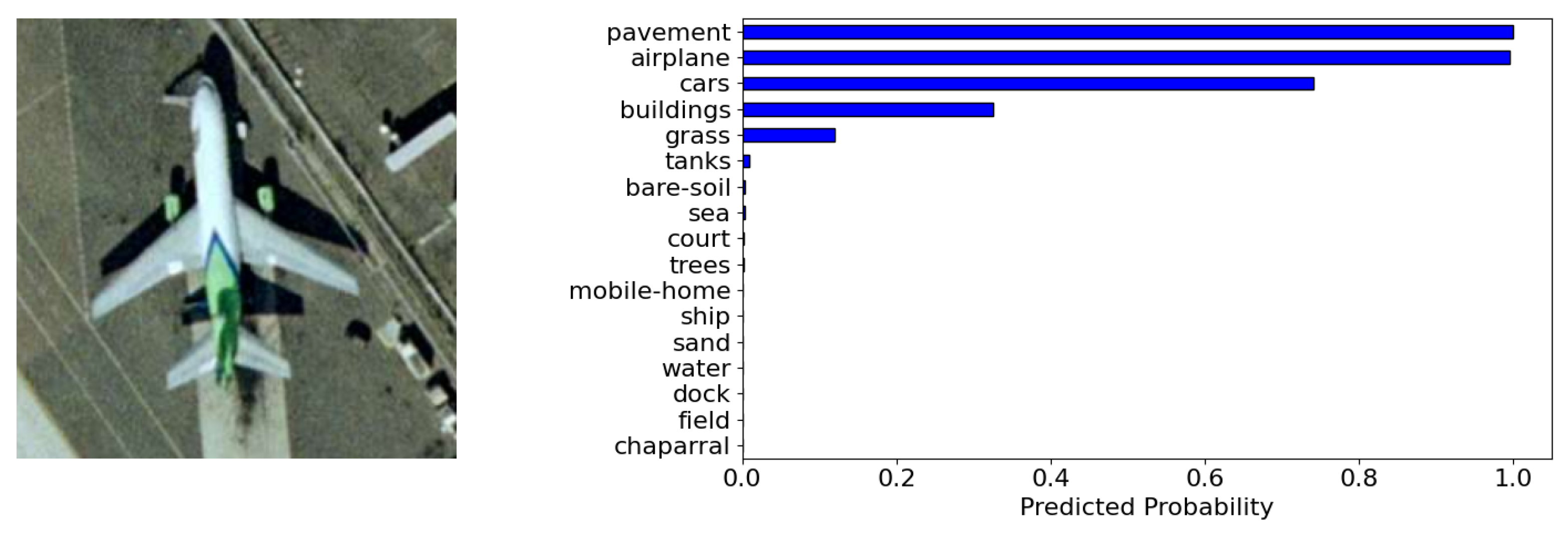
- Selvaraju, R.R.; Cogswell, M.; Das, A.; Vedantam, R.; Parikh, D.; Batra, D. Grad-CAM: Visual Explanations from Deep Networks via Gradient-Based Localization. In Proceedings of the 2017 IEEE International Conference on Computer Vision (ICCV), Venice, Italy, 22–29 October 2017; pp. 618–626. [Google Scholar]
- Boguszewski, A.; Batorski, D.; Ziemba-Jankowska, N.; Zambrzycka, A.; Dziedzic, T. LandCover.ai: Dataset for Automatic Mapping of Buildings, Woodlands and Water from Aerial Imagery. arXiv 2020, arXiv:2005.02264. [Google Scholar]
- Lin, T.Y.; Maire, M.; Belongie, S.; Hays, J.; Perona, P.; Ramanan, D.; Dollar, P.; Zitnick, L. Microsoft COCO: Common Objects in Context. In Proceedings of the Computer Vision—ECCV 2014: 13th European Conference, Zurich, Switzerland, 6–12 September 2014; Springer: Cham, Switzerland. [Google Scholar]
- Everingham, M.; Gool, L.V.; Williams, C.K.I.; Winn, J.; Zisserman, A. The Pascal Visual Object Classes (VOC) Challenge. Int. J. Comput. Vis. 2009, 88, 303–308. [Google Scholar] [CrossRef]
- Lu, X.; Zhang, Y.; Yuan, Y.; Feng, Y. Gated and Axis-Concentrated Localization Network for Remote Sensing Object Detection. IEEE Trans. Geosci. Remote Sens. 2020, 58, 179–192. [Google Scholar] [CrossRef]
- Tan, M.; Le, Q.V. EfficientNetV2: Smaller Models and Faster Training. In Proceedings of the 38th International Conference on Machine Learning (ICML 2021), Virtual Event, 18–24 July 2021; Volume 139, pp. 10096–10106. [Google Scholar]
- Wilkinson, M.D.; Dumontier, M.; Aalbersberg, I.J.; Appleton, G.; Axton, M.; Baak, A.; Blomberg, N.; Boiten, J.W.; da Silva Santos, L.B.; Bourne, P.E.; et al. The FAIR Guiding Principles for scientific data management and stewardship. Sci. Data 2016, 3, 160018. [Google Scholar] [CrossRef]
- Wang, Y.; Albrecht, C.; Ait Ali Braham, N.; Mou, L.; Zhu, X. Self-Supervised Learning in Remote Sensing: A Review. IEEE Geosci. Remote Sens. Mag. 2022, 10, 213–247. [Google Scholar] [CrossRef]
- Akiva, P.; Purri, M.; Leotta, M. Self-Supervised Material and Texture Representation Learning for Remote Sensing Tasks. In Proceedings of the IEEE/CVF Conference on Computer Vision and Pattern Recognition (CVPR), New Orleans, LA, USA, 18–24 June 2022; pp. 8203–8215. [Google Scholar]
- Manas, O.; Lacoste, A.; Giró-i-Nieto, X.; Vazquez, D.; Rodriguez, P. Seasonal Contrast: Unsupervised Pre-Training from Uncurated Remote Sensing Data. In Proceedings of the 2021 IEEE/CVF International Conference on Computer Vision (ICCV), Montreal, BC, Canada, 11–17 October 2021; IEEE Computer Society: Los Alamitos, CA, USA; pp. 9394–9403. [Google Scholar] [CrossRef]
- Wang, Y.; Braham, N.A.A.; Xiong, Z.; Liu, C.; Albrecht, C.M.; Zhu, X.X. SSL4EO-S12: A Large-Scale Multi-Modal, Multi-Temporal Dataset for Self-Supervised Learning in Earth Observation. arXiv 2022, arXiv:2211.07044. [Google Scholar]
- Buslaev, A.; Iglovikov, V.I.; Khvedchenya, E.; Parinov, A.; Druzhinin, M.; Kalinin, A.A. Albumentations: Fast and flexible image augmentations. Information 2020, 11, 125. [Google Scholar] [CrossRef]
- Oliphant, T.E. A Guide to NumPy; Trelgol Publishing: Austin, TX, USA, 2006; Volume 1. [Google Scholar]
- Kramer, O. Scikit-learn. In Machine Learning for Evolution Strategies; Springer: Cham, Switzerland, 2016; pp. 45–53. [Google Scholar]
- Szymanski, P.; Kajdanowicz, T. Scikit-multilearn: A scikit-based Python environment for performing multi-label classification. J. Mach. Learn. Res. 2019, 20, 209–230. [Google Scholar]
- Bisong, E. Matplotlib and seaborn. In Building Machine Learning and Deep Learning Models on Google Cloud Platform; Springer: Berkeley, CA, USA, 2019; pp. 151–165. [Google Scholar]
- zipp: A pathlib-Compatible Zipfile Object Wrapper. 2023. Available online: https://doc.sagemath.org/html/en/reference/spkg/zipp.html (accessed on 8 March 2023).
- dill: Serialize All of Python. 2023. Available online: https://pypi.org/project/dill/ (accessed on 8 March 2023).
- Lmdb: A Universal Python Binding for the LMDB ‘Lightning’ Database. 2023. Available online: https://lmdb.readthedocs.io/en/release/ (accessed on 8 March 2023).
- tifffile: Storing NumPY Arrays in TIFF and Read Image and Metadata from TIFF-Like Files. 2023. Available online: https://pypi.org/project/tifffile/ (accessed on 8 March 2023).
- h5py: A Pythonic Interface to the HDF5 Binary Data Format. 2023. Available online: https://www.h5py.org/ (accessed on 8 March 2023).
- Click: Command Line Interface Creation Kit. 2023. Available online: https://click.palletsprojects.com/en/8.1.x/ (accessed on 8 March 2023).
- Munch: A Dictionary Supporting Attribute-Style Access. 2023. Available online: https://morioh.com/p/bbdd8605be66 (accessed on 8 March 2023).
- Marshmallow: Simplified Object Serialization. 2023. Available online: https://marshmallow.readthedocs.io/en/stable/ (accessed on 8 March 2023).
- Detlefsen, N.S.; Borovec, J.; Schock, J.; Harsh, A.; Koker, T.; Liello, L.D.; Stancl, D.; Quan, C.; Grechkin, M.; Falcon, W. TorchMetrics—Measuring Reproducibility in PyTorch. J. Open Source Softw. 2022, 7, 4101. [Google Scholar] [CrossRef]
- Sechidis, K.; Tsoumakas, G.; Vlahavas, I. On the Stratification of Multi-Label Data. In Proceedings of the 2011 European Conference on Machine Learning and Knowledge Discovery in Databases—Volume Part III, Athens, Greece, 5–9 September 2011; Springer: Berlin/Heidelberg, Germany; pp. 145–158. [Google Scholar]
- Zhai, X.; Puigcerver, J.; Kolesnikov, A.; Ruyssen, P.; Riquelme, C.; Lucic, M.; Djolonga, J.; Pinto, A.S.; Neumann, M.; Dosovitskiy, A.; et al. A Large-scale Study of Representation Learning with the Visual Task Adaptation Benchmark. arXiv 2019, arXiv:1910.04867. [Google Scholar]
- Risojevic, V.; Stojnic, V. Do we still need ImageNet pre-training in remote sensing scene classification? arXiv 2021, 3690. [Google Scholar] [CrossRef]
- Kingma, D.P.; Ba, J. Adam: A method for stochastic optimization. arXiv 2014, arXiv:1412.6980. [Google Scholar]


| Model/Label | Background | Buildings | Woodlands | Water | Road | mIoU | Training Time |
|---|---|---|---|---|---|---|---|
| Trained from scratch | 93.813 | 80.304 | 91.952 | 94.877 | 69.190 | 86.027 | 4.5 h |
| Pre-trained on COCO | 93.857 | 80.650 | 91.964 | 95.145 | 68.846 | 86.093 | 5 h |
Disclaimer/Publisher’s Note: The statements, opinions and data contained in all publications are solely those of the individual author(s) and contributor(s) and not of MDPI and/or the editor(s). MDPI and/or the editor(s) disclaim responsibility for any injury to people or property resulting from any ideas, methods, instructions or products referred to in the content. |
© 2023 by the authors. Licensee MDPI, Basel, Switzerland. This article is an open access article distributed under the terms and conditions of the Creative Commons Attribution (CC BY) license (https://creativecommons.org/licenses/by/4.0/).
Share and Cite
Dimitrovski, I.; Kitanovski, I.; Panov, P.; Kostovska, A.; Simidjievski, N.; Kocev, D. AiTLAS: Artificial Intelligence Toolbox for Earth Observation. Remote Sens. 2023, 15, 2343. https://doi.org/10.3390/rs15092343
Dimitrovski I, Kitanovski I, Panov P, Kostovska A, Simidjievski N, Kocev D. AiTLAS: Artificial Intelligence Toolbox for Earth Observation. Remote Sensing. 2023; 15(9):2343. https://doi.org/10.3390/rs15092343
Chicago/Turabian StyleDimitrovski, Ivica, Ivan Kitanovski, Panče Panov, Ana Kostovska, Nikola Simidjievski, and Dragi Kocev. 2023. "AiTLAS: Artificial Intelligence Toolbox for Earth Observation" Remote Sensing 15, no. 9: 2343. https://doi.org/10.3390/rs15092343
APA StyleDimitrovski, I., Kitanovski, I., Panov, P., Kostovska, A., Simidjievski, N., & Kocev, D. (2023). AiTLAS: Artificial Intelligence Toolbox for Earth Observation. Remote Sensing, 15(9), 2343. https://doi.org/10.3390/rs15092343