Article

Development of a Machine Learning Forecast Model for Global Horizontal Irradiation Adapted to Tibet Based on Visible All-Sky Imaging

1
Key Laboratory for Cosmic Rays of the Ministry of Education, Tibet University, Lhasa 850000, China
2
School of Ecology and Environment, Tibet University, Lhasa 850000, China
3
Key Laboratory of Middle Atmosphere and Global Environment Observation, Institute of Atmospheric Physics, Chinese Academy of Sciences, Beijing 100029, China
4
Beijing Keytec Technology Co., Ltd., Beijing 100029, China
5
Huainan Academy of Atmospheric Sciences, Institute of Atmospheric Physics, Chinese Academy of Sciences, Huainan 232000, China
6
Institute of Urban Meteorology, Chinese Meteorological Administration (CMA), Beijing 100089, China
*
Author to whom correspondence should be addressed.
These authors contributed equally to this work.
Remote Sens. 2023, 15(9), 2340; https://doi.org/10.3390/rs15092340
Submission received: 29 March 2023 / Revised: 28 April 2023 / Accepted: 28 April 2023 / Published: 28 April 2023
(This article belongs to the Special Issue New Challenges in Solar Radiation, Modeling and Remote Sensing)

Abstract

:
The Qinghai-Tibet Plateau is rich in renewable solar energy resources. Under the background of China’s “dual-carbon” strategy, it is of great significance to develop a global horizontal irradiation (GHI) prediction model suitable for Tibet. In the radiation balance budget process of the Earth-atmosphere system, clouds, aerosols, air molecules, water vapor, ozone, CO2 and other components have a direct influence on the solar radiation flux received at the surface. For the descending solar shortwave radiation flux in Tibet, the attenuation effect of clouds is the key variable of the first order. Previous studies have shown that using Artificial intelligence (AI) models to build GHI prediction models is an advanced and effective research method. However, regional localization optimization of model parameters is required according to radiation characteristics in different regions. This study established a set of AI prediction models suitable for Tibet based on ground-based solar shortwave radiation flux observation and cloud cover observation data of whole sky imaging in the Yangbajing area, with the key parameters sensitively tested and optimized. The results show that using the cloud cover as a model input variable can significantly improve the prediction accuracy, and the RMSE of the prediction accuracy is reduced by more than 20% when the forecast horizon is 1 h compared with a model without the cloud cover input. This conclusion is applicable to a scenario with a forecast horizon of less than 4 h. In addition, when the forecast horizon is 1 h, the RMSE of the random forest and long short-term memory models with a 10-min step decreases by 46.1% and 55.8%, respectively, compared with a 1-h step. These conclusions provide a reference for studying GHI prediction models based on ground-based cloud images and machine learning.

1. Introduction

Solar energy, as a green, renewable and clean type of energy [1], is undergoing significant development [2]. However, there is great volatility in the power generation process, which presents challenges to the safe and efficient operation of the power grid [3,4]. Thus, it is critical to accurately predict solar power generation [5]. The output power is proportional to the global horizontal irradiation (GHI) received by its components [6], and the GHI is the key factor affecting the output power [7]; thus, GHI prediction has become the focus of attention in the field of solar power generation. The Qinghai-Tibet Plateau is rich in solar energy resources; the received solar energy in some areas is close to the Sahara Desert [8], so the development of solar power generation has broad prospects. At present, there is almost no research on GHI prediction in this region; thus, it is of great importance to study GHI prediction in the area. Atmospheric factors affecting GHI include clouds, aerosols, water vapor and ozone; among them, clouds and aerosols play a major role [9], while water vapor and ozone have less influence [10]. Because the pollution of the Qinghai-Tibet Plateau is less than that of inland areas, the main factor causing irradiance changes is not aerosols [11,12], and the effects of clouds are generally stronger over higher altitudes [13]; thus, clouds are the first-order influencing factor. Therefore, it is necessary to focus on the influence of clouds in GHI prediction research in this area.
Machine learning is a popular method for solar radiation prediction. A random forest (RF) model is widely used in the field of solar radiation prediction because of its better precision, low risk of overfitting, and concise hyperparameter-tuned process [14]. Sun et al. [15] used meteorological, solar radiation and air pollution index data from the Haikou, Changchun and Urumqi stations in China to predict radiation values, and the constructed RF model was superior to an empirical method. Benali et al. [16] used intelligent persistence, an artificial neural network (ANN), and a RF model to predict varying solar radiation over 1–6 h in France, and the results showed that the RF was the most effective. Hou et al. [17] used the prediction model constructed by Himawari-8 AHI data based on RF to estimate the descending short-wave radiation over China’s surface and achieved good results. Recently, long short-term memory (LSTM), an improved recurrent neural network (RNN), has been applied in the field of solar radiation. Qing and Niu [6] used 2 years of radiation data collected from Cape Verde for LSTM model training and prediction, and the RMSE was 18.34% lower than that of multilayered feedforward neural networks. Ghimire et al. [18] built a hybridized deep learning (DL) model based on the convolutional neural network (CNN) and LSTM for half-hourly global solar radiation forecasting, which was superior to other DL models. Peng et al. [19] proposed a DL model based on complete ensemble empirical mode decomposition, sine cosine algorithm, and Bi-directional LSTM to predict multi-step hourly solar radiation, which had higher prediction accuracy than the comparison model. Liu et al. [20] used 7 years of radiation data from the Atmospheric Radiation Measurement Center of the US Department of Energy to predict and evaluate solar radiation, and the results showed that LSTM had the best overall performance, with results superior to eXtreme Gradient Boosting and Autoregressive Integrated Moving Average. Clouds are a key parameter for atmospheric science related to solar energy and are one of the most significant factors influencing solar radiation prediction [21]. Therefore, Qin et al. [22] used CNN to extract the temporal variation trend of solar radiation and the spatial pattern of cloud motions from the ground-based observations and the satellite cloud images, respectively, and then predicted the GHI 1–6 h in the future based on LSTM, thus improving the accuracy of photovoltaic output forecasting. Because ground-based cloud images have higher resolution than satellite cloud images, the accuracy of prediction can be improved by extracting information from ground-based cloud images [23]. Chu et al. [24] combined sky images and an ANN to build a prediction model for predicting the 1-min average Direct Normal Irradiance, which was significantly better than a reference model. In summary, the combination of ground-based cloud images and machine learning can improve the prediction accuracy of solar radiation; however, there are few studies that take the time series data of cloud cover, which can reflect the coverage of sky clouds, as model input variables, and there is no such study on the Qinghai-Tibet Plateau. Therefore, we use ground-based visible cloud images collected in the Yangbajing area of Tibet to detect the time series data of cloud cover and build a short-term prediction model of GHI based on the machine learning algorithm to predict the 10-min average GHI over the subsequent 1–6 h, explore the input characteristics of RF and LSTM models, analyze the influence of prediction step size on model accuracy, and quantitatively study the influence of cloud cover on model accuracy.
The structure of this paper is as follows. The study area, data collection, quality control of GHI, and ground-based cloud images are introduced in Section 2. In Section 3, the research methods, including ground-based cloud image preprocessing, cloud detection, and the principles and construction of the RF and LSTM models are introduced. Finally, the experimental results, discussion, and conclusions are presented in Section 4, Section 5 and Section 6, respectively.

2. Data

2.1. General Information of the Study Area

The Yangbajing area (90°33′E, 30°05′N) is located 90 km northwest of Lhasa, Tibet, south of Nyanqing Tanggula Mountain, with an average elevation of 4300 m above sea level; it has flat terrain and is surrounded by mountains. It has a plateau monsoon semiarid climate, short spring and autumn, warm and humid summer, and cold and long winter. It is known for sunny weather and abundant sunshine year-round, with the annual sunshine time over 2800 h. The Yangbajing Total Atmosphere Observation Station under the Institute of Atmospheric Physics of the Chinese Academy of Sciences has observed the area since 2018. As the first comprehensive detection base of all neutral atmosphere and multi-elements in the Qinghai-Tibet Plateau, it has carried out simultaneous quantitative observation of the whole atmosphere (near the ground to 110 km) using high vertical resolution (10~100 m), high time resolution (1 min~1 h) and continuous multi-element observations.

2.2. Irradiance Data

The GHI data used in this study were collected using a four-component radiometer (see Figure 1a) at the Yangbajing Total Atmospheric Observation Station and measured using an MR-60 net radiometer from EKO in Japan. The instrument began measurements in April 2019, and the data collected in 2020 were used in this study. The spectral range of detection was 285–3000 nm, the output unit was W/m2, and the sampling interval was 1 min. The GHI is the strongest in summer, the second strongest in spring and the weakest in winter, demonstrating obvious seasonal variation characteristics. The diurnal variation is a “single-peak” inverted “U” distribution, reaching a peak at 13:00 and fluctuating greatly at noon. According to the irradiance characteristics, we first preprocess the data and detect the singularity of the sample after removing nan. Because of the influence of clouds and terrain [25], the instantaneous value exceeds the solar constant, and the threshold value is 1500 W/m2. The prediction error is large due to the low value of irradiance obtained before sunrise and after sunset; therefore, only the data measured between 9:00 am and 18:00 pm were considered in this study. Finally, resampling was carried out using the 10-min average value.

2.3. Ground-Based Cloud Image Data

The ground-based cloud images used in this study were acquired using the visible-light imaging subsystem of an automatic cloud cover observer (see Figure 1b) installed at the Yangbajing Total Atmospheric Observation Station. The instrument started its measurement in April 2019, and the data collected in 2020 were used in this study. The system includes a visible light imaging unit and a sun tracking unit. The visible light imaging unit consists of a super wide-angle (fisheye) lens, a camera and a super-hemispherical quartz glass cover. The super wide-angle lens directly faces the sky for all-sky shooting and imaging. The super-hemispherical cover can meet the imaging requirements of a 2π solid angle, and its equal thickness design ensures the uniformity of incident light to avoid additional distortion. The solar tracking unit is composed of a control platform, a stepper motor, a transmission mechanism and a shading ball. The control platform calculates the solar altitude angle according to the local astronomical calendar, controls the stepper motor to drive the transmission mechanism, and uses the shading ball to shade the direct incident light of the sun to protect the photosensitive elements from the direct impact of the sun while avoiding the loss of imaging details around the sun [26]. The system collected data every 10 min and obtained a full-sky RGB three-channel image with an elevation angle above 15°, a visible band, and a resolution of 4288 × 2848 pixels. Considering the imaging performance of the equipment, the local solar motion and cloud cover changes, the system needed to be synchronized with irradiance data, and only the cloud images obtained from 9:00 to 18:00 during the day were retained.

2.4. Data Set Settings

Although using more data for training will produce better results, the performance improvement may not be significant, and the training time will be increased [27], which increases the calculation cost and the difficulty of application in practice. Therefore, the GHI and ground-based cloud image data in December 2020, which includes various weather conditions in the current month without losing generalizability [4], are selected, with a time resolution of 10 min. The training set and the test set are divided using a ratio of approximately 3:1, i.e., the time series data from 1 to 23 December are selected as the training set, and the time series data from 24 to 31 December as the test set. The performance of the model does not change significantly at different dates, so no additional days are added for separate evaluation [23]. In this study, the GHI of a few time steps in advance and the cloud cover time series data obtained via cloud detection is taken as model input variables. According to the characteristics of different models, reasonable model parameters are determined by sensitivity experiments. The training, prediction and evaluation of the model are realized.

3. Methodology

The main contribution of this study is to combine the information extracted from ground-based cloud images and GHI measurements with machine learning algorithms, which includes two steps: (1) cloud cover estimation and (2) construction of the irradiance prediction model. The methods used are introduced in detail below.

3.1. Cloud Cover Estimation

3.1.1. Image Preprocessing

Figure 2a shows the original ground-based cloud image, from which we can see that buildings and surface background around the automatic cloud cover observer cause some shading of the sky, and the scattering radiation characteristics of the atmosphere make it difficult to identify clouds and clear sky near the horizon [26,28]; this introduces errors into the subsequent cloud detection and cloud amount calculation, so it is necessary to remove the ground objects from the cloud image background. Through experiments, setting the effective radius of the cloud image to 1040 pixels can eliminate the influence of the ground background to the greatest extent without affecting cloud detection. Transparent channels are added to the original three RGB image channels, pixels outside the effective radius are set as transparent, and such pixels are ignored in subsequent processing.
The projection of the shading ball and its support on the ground cloud image introduce errors into the cloud detection, so the shading ball is removed from the cloud image. The sun’s azimuth angle and zenith angle are calculated according to the shooting time and position information of the cloud image; then, the position of the sun projection on the cloud image, that is, the projection position of the shading ball, is calculated [29]. The pixels in the position and the bracket area are set to be transparent through a transparent channel, and such pixels are ignored in subsequent processing.
After the preprocessing of the original image introduced above [30] (Figure 2b), the influence of error points is eliminated for the subsequent cloud detection process, and accurate data are provided for the subsequent experimental analysis.

3.1.2. Cloud Detection

In this study, the normalized red–blue ratio (NRBR) threshold method is applied in cloud detection. The scattering of atmospheric molecules is proportional to λ 4 , so the Rayleigh scattering of molecules with shorter wavelengths increases, which leads to a blue sky with a larger blue channel (B) and a smaller red channel (R). Clouds are white in the sky, with small B values and large R values. By calculating the red–blue ratio (RBR) of each pixel in the cloud image and comparing with the threshold value [31], whether the pixel is a clear sky pixel (0) or a cloud cluster pixel (1) is evaluated, and a binary image is obtained. This method has a large error when detecting thin clouds and increased noise [29], while the NRBR, as a nonlinear monotone decreasing function of the RBR [32], can improve the image contrast and robustness to noise [30]; its formula is as follows:
NRBR = B R B + R
where the value range of NRBR is [0, 1]. Using cloud images to analyze the NRBR distribution information, through manual identification and statistical analysis of thousands of picture samples, setting the threshold value to 0.2 can maximize the cloud detection accuracy. The NRBR of each pixel of the image is calculated, and the three-channel RGB image is converted into a single-channel image. The pixel is identified as a cloud point when the NRBR is less than 0.2, while the pixel is identified as clear sky when the NRBR is greater than 0.2. The amount of cloud denoted by Cloudfraction can be obtained as follows:
Cloudfraction = N Cloud N Clear + N Cloud
where N Clear is the number of clear sky pixels, and N Cloud is the number of cloud pixels.
As shown in Figure 2c, which is the NRBR histogram of the cloud map, the sky is cloudy, and its NRBR is a bimodal distribution. The left and right peaks represent cloud and clear sky pixels, respectively, and the trough between the two peaks can be used as the critical point to distinguish cloud from clear sky pixels. Figure 2d shows the cloud detection result, and the corresponding calculated cloud cover value is 0.45.

3.1.3. Characteristics of Cloud Cover in the Yangbajing Region

Through statistical analysis of the cloud cover from 9:00 to 18:00 in 2020, the average value of cloud cover is found to be 0.55. Table 1 shows that cloudy days with cloud cover above 0.9 occur most frequently, accounting for 35.00%, followed by sunny days with cloud cover below 0.1, accounting for 23.16%. Table 2 shows that the cloud cover in this area is large in spring and summer, and the monthly average cloud cover reaches its peak in May, which is 0.79. The cloud cover is small in autumn and winter, and the monthly average reaches the minimum value of 0.12 in October, which is related to the melting of snow and ice in spring and the seasonal variation in precipitation in this area. The cloud cover fluctuates greatly in winter, and its standard deviation reaches a maximum in January and a minimum in October. Generally, the proportion of cloudy days in this area is high, the cloud cover is large, and the fluctuation of cloud cover is frequent, which leads to more sudden changes in solar radiation and makes it difficult to predict the GHI.

3.2. RF Prediction Model

An RF is an ensemble learning method in machine learning. Each tree is composed of a random subset of the original data obtained by resampling bootstrapping in the training process [33]. Each tree is fitted with a set of randomly selected features. This randomization method improves robustness and reduces the risk of overfitting [16]. Each decision tree is a basic learner, the whole forest corresponds to ensemble learning, and the average predicted value of all decision trees is the predicted result of the model.

3.2.1. Data Transformation and Feature Extraction

Because the units of GHI (X) and cloud cover (Y) are different, the first step is to normalize the data to improve the training rate and reduce the possibility of local optimization [34]. The second step is to convert the time series data into supervised learning data suitable for machine learning through a sliding window, using a GHI history time step X t 1 , X t 2 , X t 3 …… X t n and a cloud cover history time step Y t 1 , Y t 2 , Y t 3 …… Y t p as input variables, and using a GHI future time step X t + 1 , X t + 2 , X t + 3 …… X t + m (m = 1, 2, 3, 4, 5, 6 h) as the output variables [35]. The specific steps are as follows: (1) Splitting the GHI time series data into a training set, verification set and test set. (2) In advance, 1, 2, 3…… N (n < N) time sequences of time steps are used as model input variables, and the model default parameters are used to train in the training set and verify in the verification set to obtain the optimal number of input features (n), that is, the number of advance time steps (n). (3) The same method is used to determine the optimal number of input features (p) of cloud cover, that is, the number of advance time steps (p). Finally, the data are transformed into supervised learning data with (n + p)-dimensional input variables and m-dimensional output variables by reconstructing the data.

3.2.2. Parameter Tuning (Model Optimization)

Because of the characteristics of time series, the cross-validation method is not used to adjust parameters; thus, a rolling origin prediction method is used in this experiment. (1) The data set is split into a training set and test set, training is performed on the training set, and the first step in the test set is predicted. (2) The measured value of the first step in the test set is added to the training set, and the whole training set moves backward one step to ensure that the sample size of the training set is unchanged. (3) The fitting model is retrained based on the new training set, and the second step in the test set is predicted. (4) This process is repeated for the entire test set. By continuously updating the prediction origin and training set and generating predictions according to each origin, the rolling prediction times are equal to the sample size of the test set, and multiple prediction errors of the time series can be obtained to ensure the robustness of the model [36], realize the cross-validation function, and solve the overfitting problem. Finally, the prediction results are inversely normalized.

3.3. LSTM Prediction Model

LSTM is a type of RNN that is used to address the gradient disappearance problem that an RNN may encounter in long-term series training. Using the concept of a human brain neural network, each neuron is an information-processing unit. An LSTM unit consists of an input gate, an output gate and a forgetting gate. The activation function and tensor operation are used to adjust the incoming and outgoing information flow and choosing to “forget” or “remember” the input information, short-term memory and long-term memory to achieve a low error level [37].
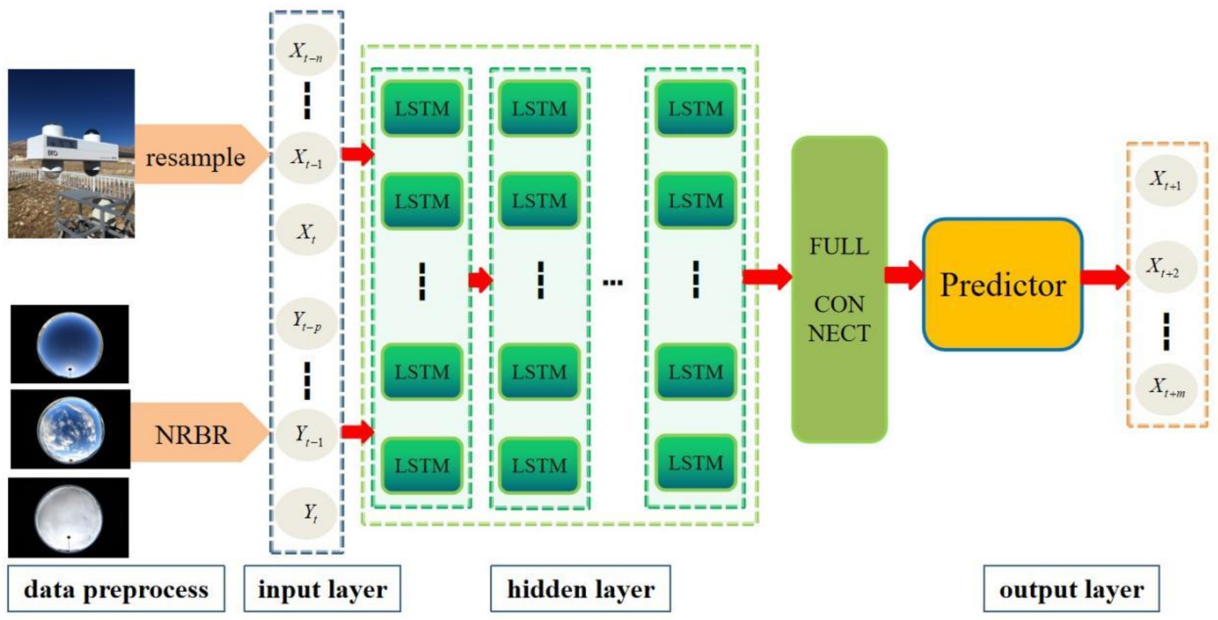
LSTM can stack multiple hidden layers, and each hidden layer can contain multiple LSTM units, which is more accurate than a single hidden layer [38]. In this study, the TensorFlow + Keras DL library is adopted, and nine hidden layer neural networks are adopted. The LSTM architecture is shown in Figure 3, and its construction process is as follows: (1) Data are normalized. (2) Using the same data transformation method as the RF, the original GHI and cloud cover time series data are reconstructed into multidimensional data of (n + p)-dimensional input variables and m-dimensional output variables. (3) For parameter adjustment (optimization), the input LSTM layer has (n + p)-dimensional input vectors, and the output layer has 6 * m (m = 1, 2, 3, 4, 5, 6) neurons according to the forecast horizon, the maximum number of neurons in the hidden layer is set to 220, the number of neurons in all hidden layers is the same, all layers adopt a Rectified Linear Unit activation function, the optimizer uses the Adaptive Moment Estimation random optimization algorithm, the maximum training epoch is set to 200, and the batch parameter is set to 55. By minimizing the RMSE on the verification set, the model hyperparameters, such as the best-hidden layer neuron with a forecast horizon of 1–6 h and the training epoch, are adjusted via grid search. Because the characteristics of time series data are not cross-validated and the model will randomly initialize weights, each set of parameters is run 30 times, and the average value of the operation results is used to evaluate the model. In addition, a dropout layer is used after each hidden layer, the dropout rate is set to 0.1, and the weight is randomly returned to zero to randomly ignore the neurons and their connections in the hidden layer [39]. The above methods can effectively avoid the model overfitting problem, make the model more robust, and improve the generalization of the model. (4) The results are inversely normalized.

3.4. Evaluation Index

The root mean square error (RMSE) is more sensitive to large deviations between predicted values and measured values. Therefore, when a set of predicted values contains multiple large errors, the RMSE is more suitable for model evaluation than other indicators, which is usually the case for solar radiation prediction, and the RMSE is dominant in the fields of prediction, statistics, econometrics and meteorology [40]. Therefore, the RMSE and normalized root mean square error (NRMSE) are used to evaluate the performance of the model in this study, and the RMSE and NRMSE are calculated according to:
RMSE = 1 N t = 1 N ( y t y ^ t ) 2
NRMSE = RMSE y t ¯ × 100
where y t , y ^ t , and y t ¯ are the measured, predicted and measured mean values of the GHI at time t, respectively, and N is the number of samples in the data set. The smaller the RMSE and NRMSE, the higher the model accuracy.

4. Results

4.1. Model Input Feature Analysis

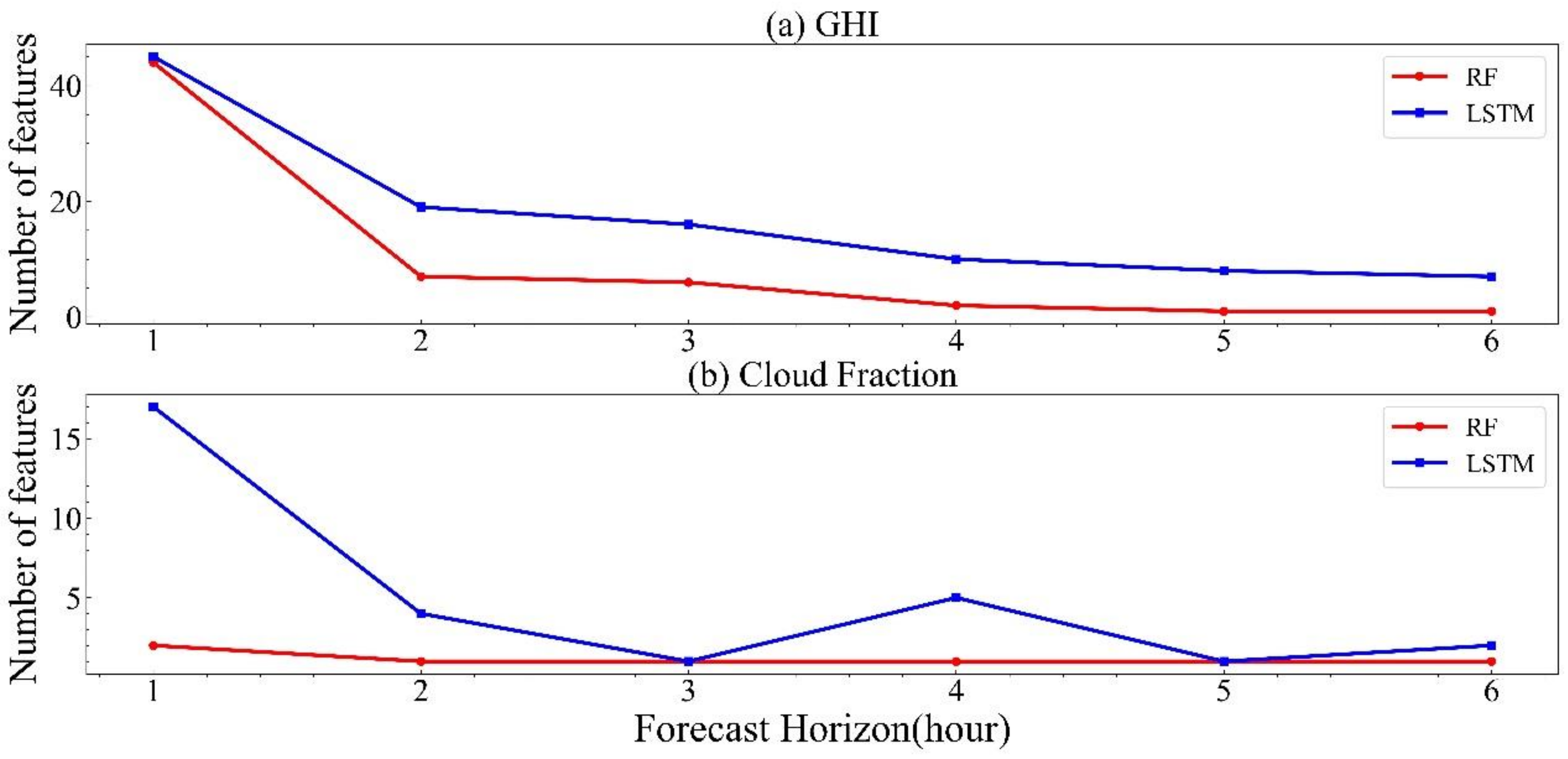
In this study, the historical time series of the GHI and cloud cover are taken as the model input variables, and the number of input features, that is, the number of advance time steps, is very important. Exploring the number of advance time steps required by different models under different forecast horizons can provide a reference for building GHI prediction models based on machine learning. In this study, the number of input features selected is the number of advance time steps when selecting the minimum RMSE value. As shown in Table 3 and Figure 4, the number of GHI input features gradually decreases with the increasing forecast horizon, which gradually increases from 1 h to 6 h, the RF model gradually decreases from 44 to 1, and the LSTM model gradually decreases from 45 to 7. There is no similar law in the number of input features of cloud cover, but it is most often equal to 1, which indicates that the cloud cover one step ahead (10 min ahead) is crucial to the irradiance prediction, that is, the latest input value of cloud cover is the best index of the future value of irradiance [41]. In addition, when the same input variables are in the same forecast horizon, the number of LSTM model input features is larger than that of the RF, which indicates that the LSTM model needs more dimensional data to train and fit the model compared with the RF.

4.2. Analysis of the Forecast Horizon and Step Size

Previous studies have shown that a difference in the prediction step size will affect the accuracy of the model [42]. Therefore, this study designed comparative experiments with different prediction step sizes. The data are resampled to the one-hour average value, and the prediction results are compared with the prediction step size of 10 min to explore the influence of the step size on the model. The prediction step size changes from 10 min to 1 h, and the sample size changes to 1/6 of the original. The sample size of the training set is the decisive variable of the model generalization ability, and the sample size will affect the learning and training effect of the model. Therefore, the data from August to December are selected for the experiment, with the data from August to November selected as the training set, and the data from December selected as the test set, to ensure that the sample sizes of the two experiments are close.
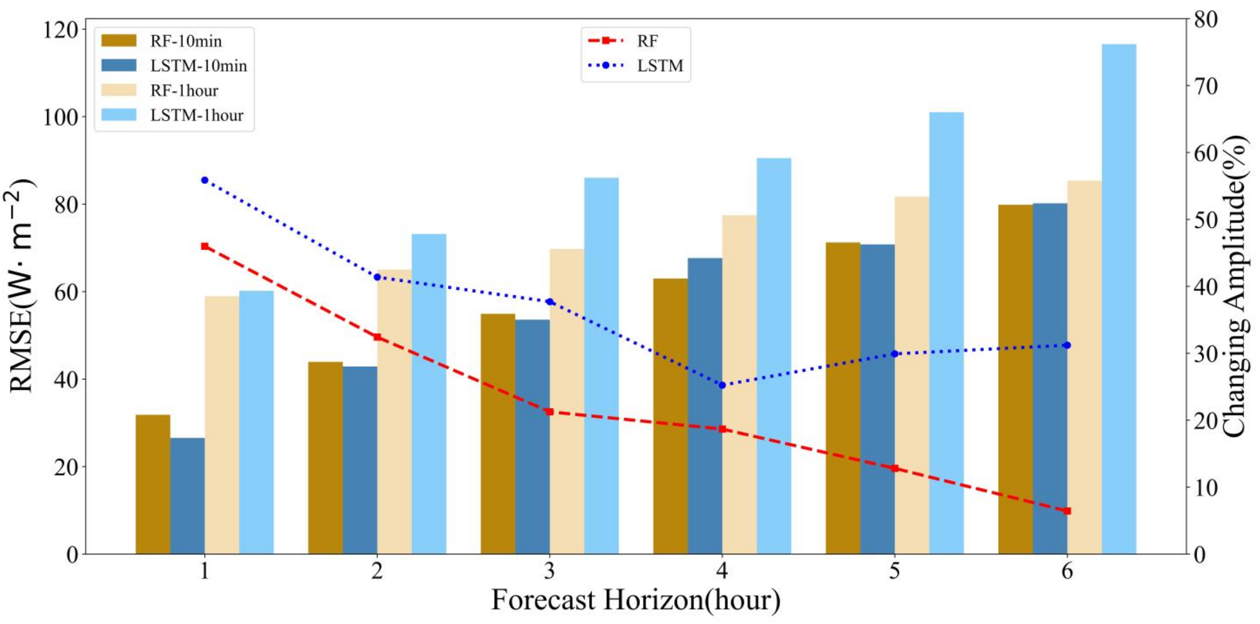
Table 4 and Table 5 and Figure 5 show that when the prediction step size is 10 min and the forecast horizon is gradually increased from 1 h to 6 h, the RMSE of the RF model gradually increases from 31.84 W/m2 to 79.85 W/m2, and the NRMSE gradually increases from 6.07% to 15.98%. The RMSE of the LSTM model increased gradually from 26.56 W/m2 to 80.19 W/m2, and the NRMSE increased gradually from 5.05% to 15.84%. When the prediction step size was 1 h and the forecast horizon increased gradually from 1 h to 6 h, the RMSE of the RF model increased gradually from 58.95 W/m2 to 85.35 W/m2, and the NRMSE increased gradually from 12.46% to 18.19%. The RMSE of the LSTM model increased gradually from 60.18 W/m2 to 116.58 W/m2, and the NRMSE increased gradually from 12.73% to 24.91%. With the increase in the forecast horizon, the errors of the RF and LSTM models gradually increased under both prediction step sizes [16], possibly because more meteorological information was lost in the longer forecast horizon [43], and the sky may have changed greatly, especially in cloudy weather [27].
It can be seen from Table 4 that under the same forecast horizon, the accuracy of the RF and LSTM models with a prediction step size of 10 min is higher than that with a prediction step size of 1 h. From the broken line of the RMSE amplitude change in Figure 5, it can be seen that the forecast horizon gradually increases from 1 h to 6 h, and the RMSE of the RF model decreases by 45.99%, 32.42%, 21.26%, 18.68%, 12.81% and 6.44% compared with 1 h when the prediction step size is 10 min. The LSTM model decreases by 55.87%, 41.38%, 37.71%, 25.24%, 29.92% and 31.21%, respectively. This shows that the shorter the prediction step size of the data, that is, the higher the time sampling frequency, the higher the prediction accuracy of the model will be [44]. This may be because a higher sampling frequency and time resolution can obtain a more accurate and representative average value, as the changes of solar irradiance caused by clouds are more likely to be captured [45]. Moreover, the shorter the forecast horizon, the greater the performance improvement will be. Under the same circumstances, the improvement of the LSTM model is greater than that of the RF model. The accuracy of different models under different prediction step sizes is also different. Under a 1-h prediction step size, the accuracy of the RF model is higher than that of the LSTM model, and the performance gap becomes larger with the increasing forecast horizon. The accuracy of the LSTM model is higher than that of the RF model in most cases under the prediction step size of 10 min, which shows that the LSTM model is more suitable for data with a high time resolution. This is because neural networks can better deal with complex nonlinear problems and can better reflect the rapidly changing sky conditions [28].
The above results show that the difference in forecast horizon and step size has different influences on different models; thus, the model should be selected according to the data resolution, forecast horizon and accuracy requirements.

4.3. Influence of Cloud Cover on Model Accuracy

Clouds are the most important atmospheric phenomenon affecting GHI [43]. Using the cloud cover as the model input variable can improve the prediction accuracy, but there are few quantitative studies on the level of improvement. Therefore, the control experiments with or without cloud cover time series as the model input variable show that the model parameters remain unchanged.
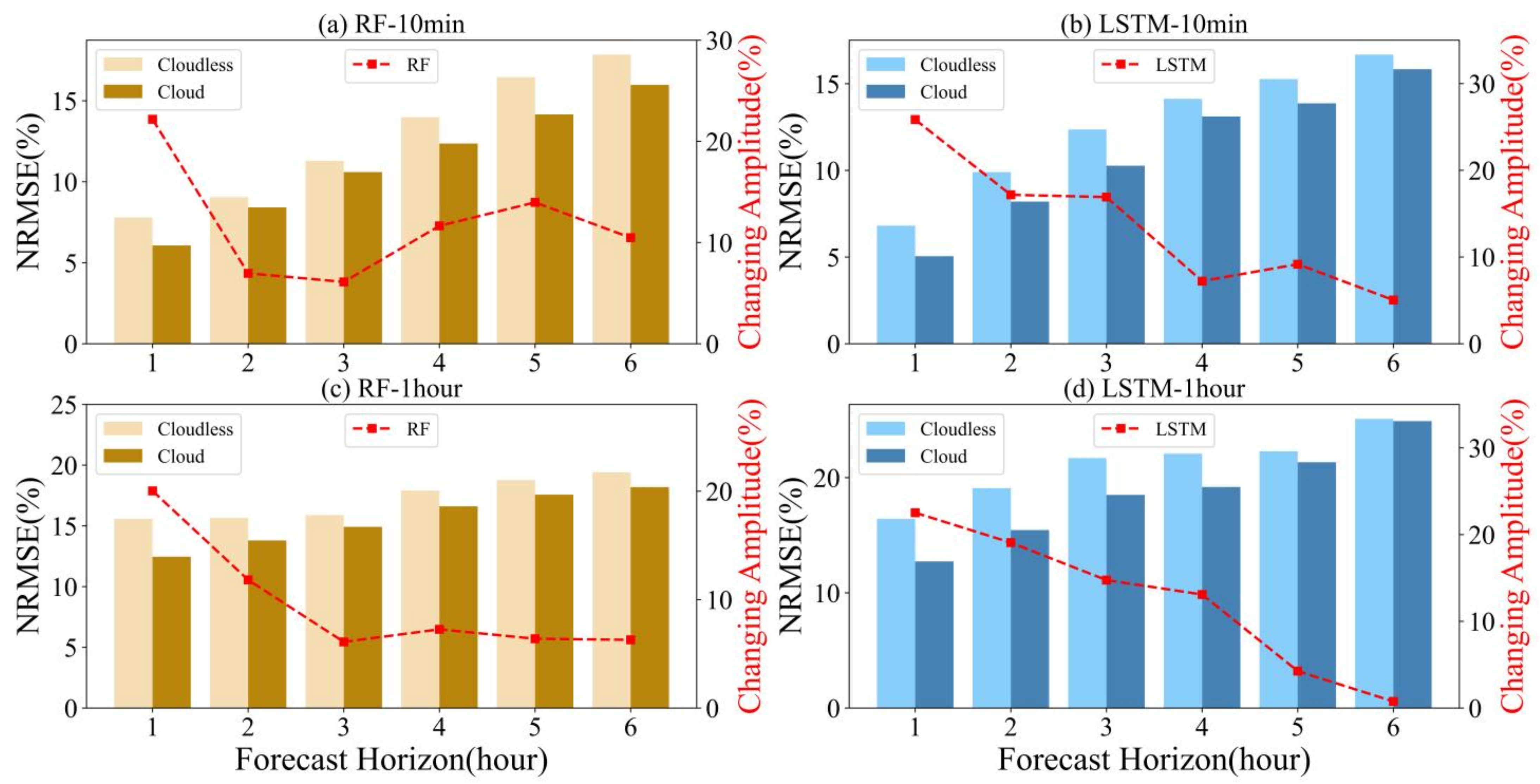
As shown in Table 5 and Figure 6, the model performance is greatly improved by adding cloud cover time series as input variables. When the prediction step size is 10 min, the forecast horizon gradually increases from 1 h to 6 h, and the NRMSE of the RF model decreases by 22.18%, 6.96%, 6.11%, 11.65%, 13.97% and 10.48%, respectively, and that of the LSTM model decreases by 25.84%, 17.17%, 16.91%, 7.22%, 9.17% and 5.04%. When the prediction step size is 1 h, the NRMSE of the RF model decreases by 20.03%, 11.82%, 6.1%, 7.26%, 6.39% and 6.29%, and that of the LSTM model decreases by 22.52%, 19.07%, 14.75%, 13.09%, 4.26% and 0.76%. In particular, when the forecast horizon is 1 h, the NRMSE of the two models decreases by more than 20% under the different prediction step sizes. In addition, although the forecast horizon is 2 h, the improvement in the model performance of the RF model under a 10-min step size is greater than that under a 1-h step size.
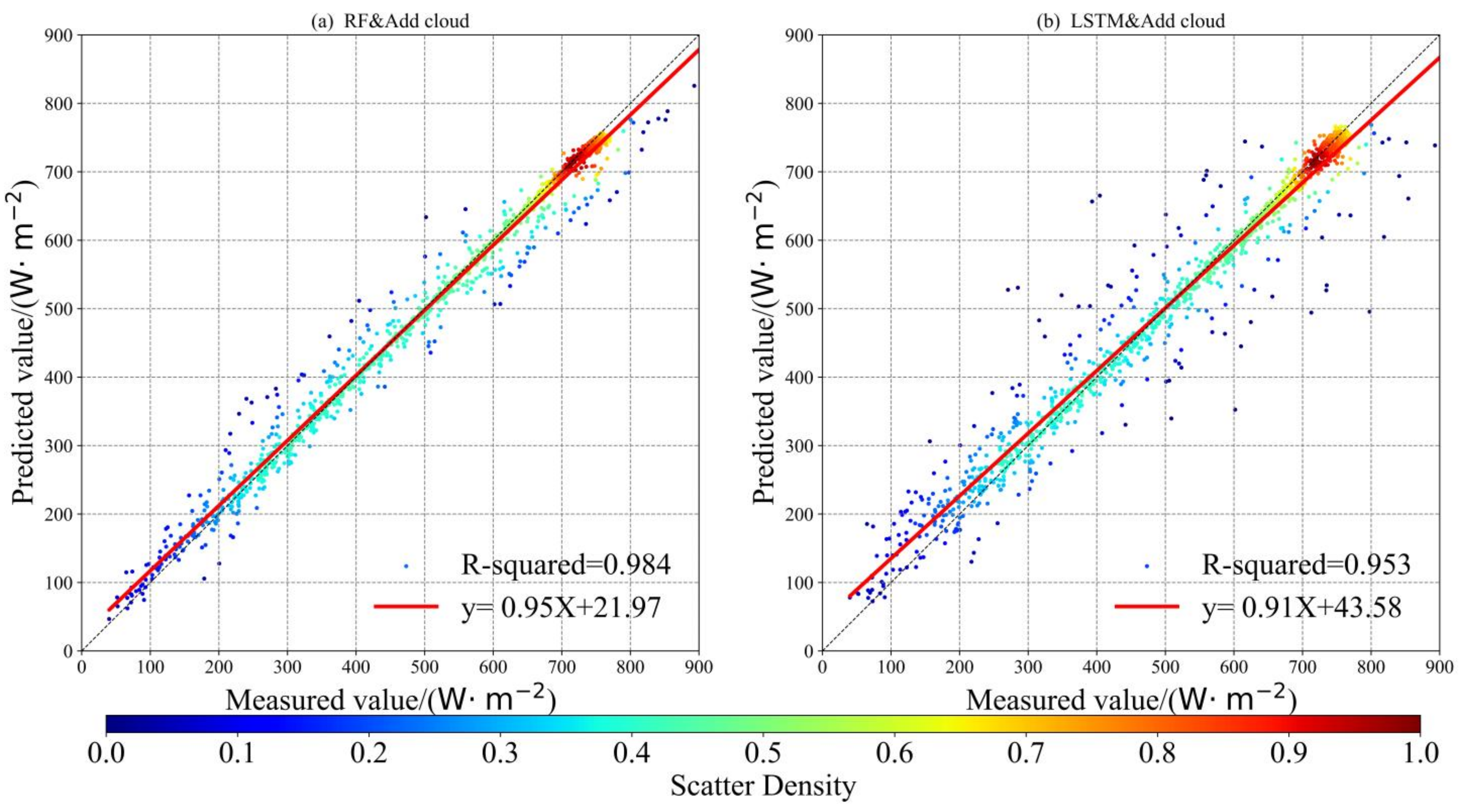
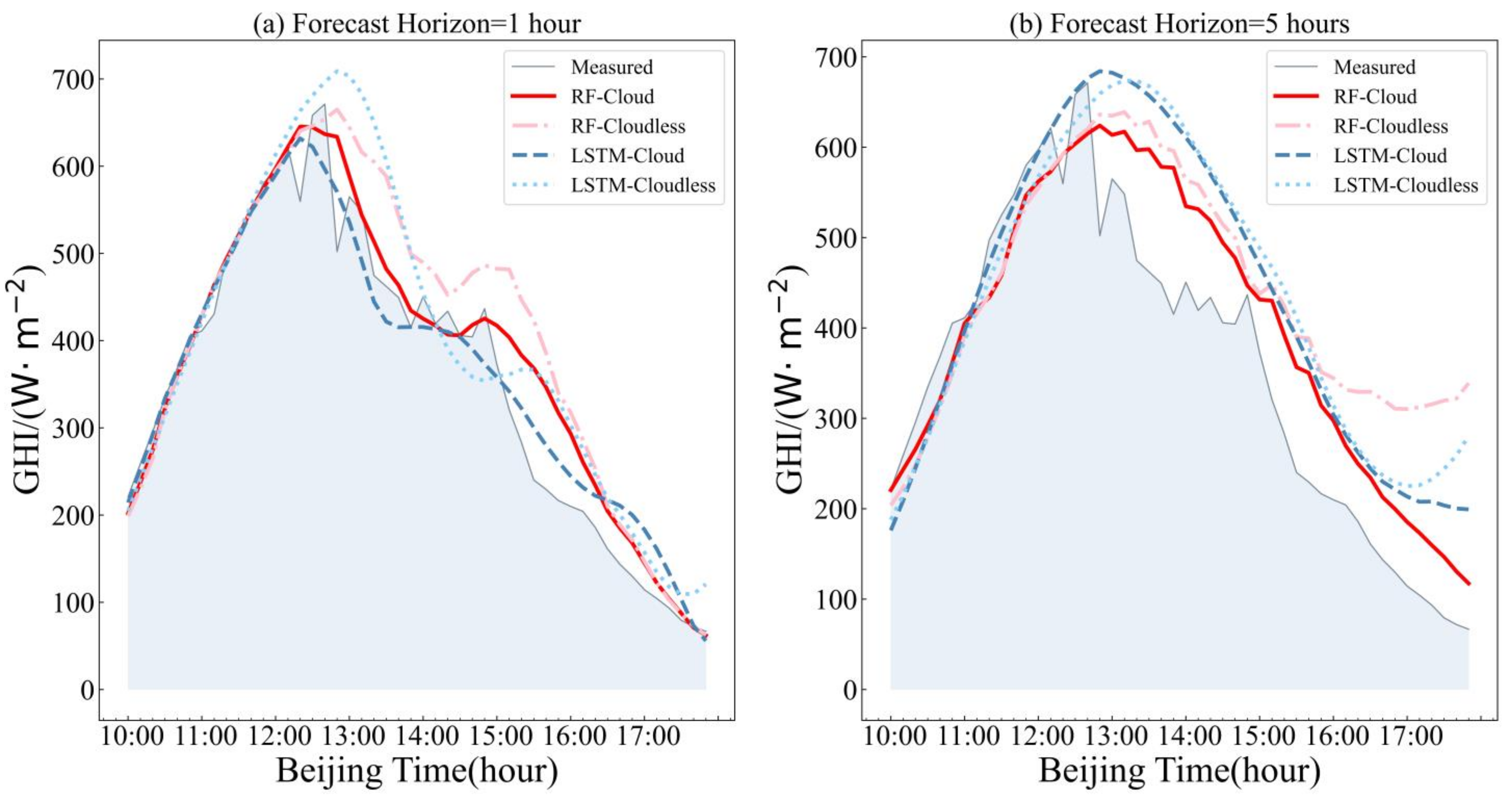
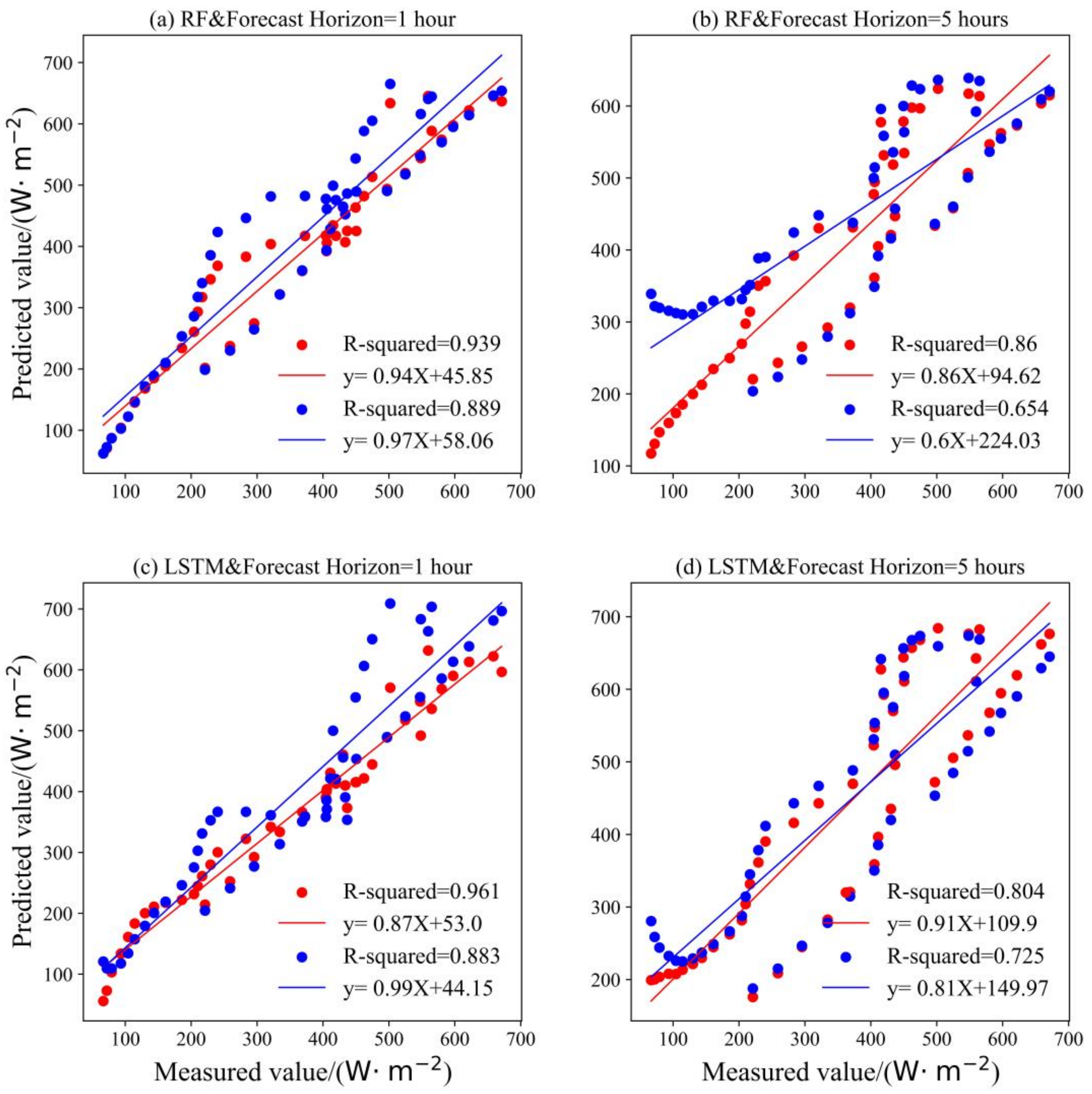
The above results show that the accuracy of the model can be improved by adding cloud cover, and the maximum improvement is the forecast horizon of 1 h; as shown in Figure 7, the prediction step size is 10 min, the forecast horizon is 1 h, and the R-squared of both models is above 0.95, indicating a high degree of fit. This influence will gradually change with the change in the forecast horizon. Figure 8 shows that from 12:10 to 14:00, the cloud cover gradually increases from 0.18 to 1, and the GHI changes abruptly. In Figure 8a, the forecast horizon is 1 h compared with the light red curve, the dark red curve is obviously closer to the gray measured curve, and the changing trend is more similar to the measured value, which can more accurately reflect the sudden change in GHI (capture the GHI trend). Even if the appearance of clouds changes greatly, cloud cover can accurately reflect the influence of its change on solar radiation. At this time, adding cloud cover as an RF model input variable can significantly improve the model accuracy. In Figure 8b, the forecast horizon is 5 h, and the dark red curve and light red curve are close, which are obviously far away from the gray measured curves. Both models cannot accurately predict when the GHI fluctuates greatly, which shows that the cloud cover can no longer accurately reflect the influence of its change on GHI at this time, and adding cloud cover as an RF model input variable can no longer significantly improve the accuracy of the model. The conclusion of the LSTM model is the same as that of the RF model. Figure 9 is a scatter diagram of the measured values and the predicted values of the model on the same day. Figure 9a,b show the forecast horizon of the RF model for 1 h and 5 h, respectively, and Figure 9c,d show the forecast horizon of the LSTM model for 1 h and 5 h, respectively. Figure 9a,b show that the coefficient of determination (R-squared) is the largest when the cloud cover is used as the RF model input variable and the forecast horizon is 1 h, reaching 0.939, and the fitting degree of the model is the highest. Figure 9c,d show that the coefficient of determination (R-squared) is the largest when the cloud cover is used as the LSTM model input variable and the forecast horizon is 1 h, reaching 0.961, and the fitting degree of the model is the highest. Both models show that a forecast horizon of 1 h and adding cloud cover as an input variable can significantly improve the model accuracy compared to a forecast horizon of 5 h and the model unable to identify the abrupt radiation change caused by cloud cover. Therefore, taking cloud cover as the model input variable is suitable for predicting scenes with a duration of less than 4 h.

5. Discussion

This study shows that adding cloud cover time series as model input variables can greatly improve the accuracy of GHI prediction, which shows that solar irradiance prediction should not only rely on data-driven machine learning and DL models but also be considered from the perspective of physics. Clouds are the most important atmospheric phenomena affecting solar radiation, and clouds can affect solar radiation through cloud cover. Therefore, the ground-based cloud image is combined with machine learning and DL, and the cloud cover time series data obtained from cloud detection are taken as the input variable of the model. By introducing a physics-based prediction model, the contribution of cloud cover is distinguished, and the influence of cloud cover on the model accuracy is quantitatively studied, which improves the interpretability of the model and proves the importance and practicability of incorporating physics into the model in improving the prediction accuracy. In practical application, it is difficult to obtain a large number of ground-based cloud images and GHI data. In order to reduce the difficulty in practical application, this study selects one month of GHI and ground-based cloud images for experiments, but the difference in sample size will affect the prediction accuracy of the model and then affect the research results. For example, from Table 2, it can be seen that the monthly average of cloud cover is larger in spring and summer, both above 0.6, while it is smaller in autumn and winter, and the fluctuation of cloud cover is different in different months. Generally speaking, the greater the cloud cover, the greater the fluctuation, and the difficulty of model prediction increases. Therefore, choosing the data of different months as the training set of the model for learning and fitting, the prediction accuracy is different. In view of the possible impact of sample size differences on the research results, this study also uses the data from other months for the same experiment and obtains similar results, which verifies the effectiveness and universality of the proposed method.
One of the key points of this study is to take the ground-based visible cloud image as the input variable of the model, with the traditional NRBR threshold method adopted for cloud detection. This method is not sufficiently accurate to identify thin clouds and different types of clouds; various types of clouds have different influences on solar radiation [46]. Therefore, future work will focus on the accurate identification of different types of clouds, giving weights according to their respective physical characteristics and further improving the prediction accuracy. At the same time, in the preprocessing of cloud images, the background of ground objects and shading balls that may cause cloud detection errors are simply deducted, which will remove real information on cloud images. In the future, we can consider image restoration to reduce errors. In addition, the aerosol is also an important factor affecting irradiance. Because the aerosol content in the Qinghai-Tibet Plateau is small, the influence of aerosol is not considered in this study. The aerosol content in low altitude areas is large, so aerosol optical depth and other data can be input into the model constructed by this study to further reduce the uncertainty of GHI prediction.

6. Conclusions

In this study, a short-term prediction GHI model based on machine learning is explored. The model is based on RF and LSTM algorithms and takes the GHI and cloud cover time series data as input variables to predict the GHI over the subsequent 1–6 h, which is verified using monitoring data in the Yangbajing area of the Qinghai-Tibet Plateau. The experimental results show that cloud cover is the main factor affecting solar radiation reaching the surface, and the prediction accuracy of the model can be greatly improved by adding cloud cover time series as an input variable. When the forecast horizon is 1 h, the NRMSE of the RF and LSTM models decreases by more than 20% compared with that of the model without the cloud cover input variable. However, when the forecast horizon exceeds 4 h, the cloud cover can no longer accurately reflect the influence of its change on GHI. At this time, adding cloud cover as an input variable can no longer significantly improve the accuracy of the model, so the input cloud cover variable is suitable for a forecast horizon within 4 h. At the same time, a comparative experiment shows that the prediction step size has a great influence on the model accuracy. When the forecast horizon is 1 h, the RMSE of the RF and LSTM models decreases by 45.99% and 55.87%, respectively, under a 10-min prediction step size compared with that under a 1-h step size, and different models are also affected by the prediction step size under different forecast horizons. In addition, the number of input features of input variables, that is, the number of advance time steps, is critical to the prediction accuracy of the model. Determining the number of input features of different models under different forecast horizons can provide a reference for building high-precision prediction models.
Through this study, it is verified that RF and LSTM machine learning algorithms are feasible for building a short-term GHI prediction model in the Tibet area. By adding cloud cover input variables as well as selecting high-time resolution data and an appropriate number of input features, the model error can be greatly reduced, which provides a new method with high precision for solar power generation and GHI prediction.

Author Contributions

Conceptualization, Y.W., L.W. and T.C.; methodology, Y.W., L.W. and T.C.; software, Y.W. and L.W.; validation, Y.W., L.W. and T.C.; formal analysis, Y.W., L.W., T.C. and N.C., D.W. and H.M.; investigation, L.W., T.C., N.C., D.W., H.M., M.L. and W.Z.; resources, Y.W., L.W., T.C., M.L., W.Z., J.L., X.H. and S.J.; data curation, Y.W., L.W., T.C., J.L., X.H., S.J., L.L. and Y.P.; writing—original draft preparation, L.W. and T.C.; writing—review and editing, all authors; funding acquisition, Y.W. and T.C. All authors have read and agreed to the published version of the manuscript.

Funding

This work was funded by the Second Tibetan Plateau Scientific Expedition and Research Program of China under Grant 2019QZKK0604, by the National Key Research and Development Program of China under Grant 2021YFC2203203, by the Young Doctor Development Program of Tibet University under Grant zdbs202201, and by the High-level Personnel Training Program of Tibet University under Grant 2020-GSP-B009.

Data Availability Statement

The data that support the findings of this study are available from the corresponding author upon reasonable request.

Conflicts of Interest

The authors declare no conflict of interest.

References

  1. Zang, H.; Cheng, L.; Ding, T.; Cheung, K.W.; Wang, M.; Wei, Z.; Sun, G. Estimation and validation of daily global solar radiation by day of the year-based models for different climates in China. Renew. Energy 2019, 135, 984–1003. [Google Scholar] [CrossRef]
  2. Urban, F.; Geall, S.; Wang, Y. Solar PV and solar water heaters in China: Different pathways to low carbon energy. Renew. Sustain. Energy Rev. 2016, 64, 531–542. [Google Scholar] [CrossRef]
  3. Murata, A.; Ohtake, H.; Oozeki, T. Modeling of uncertainty of solar irradiance forecasts on numerical weather predictions with the estimation of multiple confidence intervals. Renew. Energy 2018, 117, 193–201. [Google Scholar] [CrossRef]
  4. Yang, Z.; Mourshed, M.; Liu, K.; Xu, X.; Feng, S. A novel competitive swarm optimized RBF neural network model for short-term solar power generation forecasting. Neurocomputing 2020, 397, 415–421. [Google Scholar] [CrossRef]
  5. Yang, L.; Gao, X.; Li, Z.; Jia, D.; Jiang, J. Nowcasting of Surface Solar Irradiance Using FengYun-4 Satellite Observations over China. Remote Sens. 2019, 11, 1984. [Google Scholar] [CrossRef]
  6. Qing, X.; Niu, Y. Hourly day-ahead solar irradiance prediction using weather forecasts by LSTM. Energy 2018, 148, 461–468. [Google Scholar] [CrossRef]
  7. Wang, F.; Zhen, Z.; Liu, C.; Mi, Z.; Hodge, B.; Shafie-khah, M.; Catalão, J.P.S. Image phase shift invariance based cloud motion displacement vector calculation method for ultra-short-term solar PV power forecasting. Energy Convers. Manag. 2018, 157, 123–135. [Google Scholar] [CrossRef]
  8. Li, Z.; Zhang, G.; Li, D.; Zhou, J.; Li, L.; Li, L. Application and development of solar energy in building industry and its prospects in China. Energy Policy 2007, 35, 4121–4127. [Google Scholar] [CrossRef]
  9. Wild, M. Global dimming and brightening: A review. J. Geophys. Res. 2009, 114. [Google Scholar] [CrossRef]
  10. Wang, Q.; Zhang, H.; Yang, S.; Chen, Q.; Zhou, X.; Shi, G.; Cheng, Y.; Wild, M. Potential Driving Factors on Surface Solar Radiation Trends over China in Recent Years. Remote Sens. 2021, 13, 704. [Google Scholar] [CrossRef]
  11. Yang, K.; Ding, B.; Qin, J.; Tang, W.; Lu, N.; Lin, C. Can aerosol loading explain the solar dimming over the Tibetan Plateau? Geophys. Res. Lett. 2012, 39. [Google Scholar] [CrossRef]
  12. Yang, K.; Wu, H.; Qin, J.; Lin, C.; Tang, W.; Chen, Y. Recent climate changes over the Tibetan Plateau and their impacts on energy and water cycle: A review. Glob. Planet. Chang. 2014, 112, 79–91. [Google Scholar] [CrossRef]
  13. Fountoulakis, I.; Kosmopoulos, P.; Papachristopoulou, K.; Raptis, I.; Mamouri, R.; Nisantzi, A.; Gkikas, A.; Witthuhn, J.; Bley, S.; Moustaka, A.; et al. Effects of Aerosols and Clouds on the Levels of Surface Solar Radiation and Solar Energy in Cyprus. Remote Sens. 2021, 13, 2319. [Google Scholar] [CrossRef]
  14. Wu, H.; Ying, W. Benchmarking Machine Learning Algorithms for Instantaneous Net Surface Shortwave Radiation Retrieval Using Remote Sensing Data. Remote Sens. 2019, 11, 2520. [Google Scholar] [CrossRef]
  15. Sun, H.; Gui, D.; Yan, B.; Liu, Y.; Liao, W.; Zhu, Y.; Lu, C.; Zhao, N. Assessing the potential of random forest method for estimating solar radiation using air pollution index. Energy Convers. Manag. 2016, 119, 121–129. [Google Scholar] [CrossRef]
  16. Benali, L.; Notton, G.; Fouilloy, A.; Voyant, C.; Dizene, R. Solar radiation forecasting using artificial neural network and random forest methods: Application to normal beam, horizontal diffuse and global components. Renew. Energy 2019, 132, 871–884. [Google Scholar] [CrossRef]
  17. Hou, N.; Zhang, X.; Zhang, W.; Wei, Y.; Jia, K.; Yao, Y.; Jiang, B.; Cheng, J. Estimation of Surface Downward Shortwave Radiation over China from Himawari-8 AHI Data Based on Random Forest. Remote Sens. 2020, 12, 181. [Google Scholar] [CrossRef]
  18. Ghimire, S.; Deo, R.C.; Raj, N.; Mi, J. Deep solar radiation forecasting with convolutional neural network and long short-term memory network algorithms. Appl. Energy 2019, 253, 113541. [Google Scholar] [CrossRef]
  19. Peng, T.; Zhang, C.; Zhou, J.; Nazir, M.S. An integrated framework of Bi-directional long-short term memory (BiLSTM) based on sine cosine algorithm for hourly solar radiation forecasting. Energy 2021, 221, 119887. [Google Scholar] [CrossRef]
  20. Liu, W.; Liu, Y.; Zhang, T.; Han, Y.; Zhou, X.; Xie, Y.; Yoo, S. Use of physics to improve solar forecast: Part II, machine learning and model interpretability. Sol. Energy 2022, 244, 362–378. [Google Scholar] [CrossRef]
  21. Yang, D.; Wang, W.; Xia, X. Related articles that may interest you. Adv. Atmos. Sci. 2022, 8, 1239–1251. [Google Scholar] [CrossRef]
  22. Qin, J.; Jiang, H.; Lu, N.; Yao, L.; Zhou, C. Enhancing solar PV output forecast by integrating ground and satellite observations with deep learning. Renew. Sustain. Energy Rev. 2022, 167, 112680. [Google Scholar] [CrossRef]
  23. Caldas, M.; Alonso-Suárez, R. Very short-term solar irradiance forecast using all-sky imaging and real-time irradiance measurements. Renew. Energy 2019, 143, 1643–1658. [Google Scholar] [CrossRef]
  24. Chu, Y.; Li, M.; Pedro, H.T.C.; Coimbra, C.F.M. Real-time prediction intervals for intra-hour DNI forecasts. Renew. Energy 2015, 83, 234–244. [Google Scholar] [CrossRef]
  25. King, J.C. Longwave atmospheric radiation over Antarctica. Antarct. Sci. 1996, 8, 105–109. [Google Scholar] [CrossRef]
  26. Long, C.N.; Sabburg, J.M.; Calbo, J.; Pages, D. Retrieving Cloud Characteristics from Ground-Based Daytime Color All-Sky Images. J. Atmos. Ocean. Technol. 2006, 23, 633–652. [Google Scholar] [CrossRef]
  27. Zhang, J.; Verschae, R.; Nobuhara, S.; Lalonde, J. Deep photovoltaic nowcasting. Sol. Energy 2018, 176, 267–276. [Google Scholar] [CrossRef]
  28. Jiang, J.; Lv, Q.; Gao, X. The Ultra-Short-Term Forecasting of Global Horizonal Irradiance Based on Total Sky Images. Remote Sens. 2020, 12, 3671. [Google Scholar] [CrossRef]
  29. Heinle, A.; Macke, A.; Srivastav, A. Automatic cloud classification of whole sky images. Atmos. Meas. Tech. 2010, 3, 557–567. [Google Scholar] [CrossRef]
  30. Li, Q.; Lu, W.; Yang, J. A Hybrid Thresholding Algorithm for Cloud Detection on Ground-Based Color Images. J. Atmos. Ocean. Technol. 2011, 28, 1286–1296. [Google Scholar] [CrossRef]
  31. Shields, J.; Karr, M.E.; Burden, A.; Johnson, R.W.; Hodgkiss, W.S. Continuing Support of Cloud Free Line of Sight Determination Including Whole Sky Imaging of Clouds; University of California: San Diego, CA, USA, 2007. [Google Scholar]
  32. Ghonima, M.S.; Urquhart, B.; Chow, C.W.; Shields, J.E.; Cazorla, A.; Kleissl, J. A method for cloud detection and opacity classification based on ground based sky imagery. Atmos. Meas. Tech. 2012, 5, 2881–2892. [Google Scholar] [CrossRef]
  33. Breiman, L. Random Forests. Mach. Learn. 2001, 45, 5–32. [Google Scholar] [CrossRef]
  34. Jang, J.; Sohn, E.; Park, K. Estimating Hourly Surface Solar Irradiance from GK2A/AMI Data Using Machine Learning Approach around Korea. Remote Sens. 2022, 14, 1840. [Google Scholar] [CrossRef]
  35. Azimi, R.; Ghayekhloo, M.; Ghofrani, M. A hybrid method based on a new clustering technique and multilayer perceptron neural networks for hourly solar radiation forecasting. Energy Convers. Manag. 2016, 118, 331–344. [Google Scholar] [CrossRef]
  36. Tashman, L.J. Out-of-sample tests of forecasting accuracy: An analysis and review. Int. J. Forecast. 2000, 16, 437–450. [Google Scholar] [CrossRef]
  37. Hochreiter, S.; Schmidhuber, J. Long Short-Term Memory. Neural Comput. 1997, 8, 1735–1780. [Google Scholar] [CrossRef]
  38. Yu, L.; Qu, J.; Gao, F.; Tian, Y. A Novel Hierarchical Algorithm for Bearing Fault Diagnosis Based on Stacked LSTM. Shock Vib. 2019, 2019, 2756284. [Google Scholar] [CrossRef]
  39. Srivastava, S.; Lessmann, S. A comparative study of LSTM neural networks in forecasting day-ahead global horizontal irradiance with satellite data. Sol. Energy 2018, 162, 232–247. [Google Scholar] [CrossRef]
  40. Gneiting, T. Making and Evaluating Point Forecasts. J. Am. Stat. Assoc. 2011, 494, 746–762. [Google Scholar] [CrossRef]
  41. Chu, Y.; Urquhart, B.; Gohari, S.M.I.; Pedro, H.T.C.; Kleissl, J.; Coimbra, C.F.M. Short-term reforecasting of power output from a 48 MWe solar PV plant. Sol. Energy 2015, 112, 68–77. [Google Scholar] [CrossRef]
  42. Zhang, J.; Zhao, L.; Deng, S.; Xu, W.; Zhang, Y. A critical review of the models used to estimate solar radiation. Renew. Sustain. Energy Rev. 2017, 70, 314–329. [Google Scholar] [CrossRef]
  43. Yang, D.; Jirutitijaroen, P.; Walsh, W.M. Hourly solar irradiance time series forecasting using cloud cover index. Sol. Energy. 2012, 86, 3531–3543. [Google Scholar] [CrossRef]
  44. Blaga, R. The impact of temporal smoothing on the accuracy of separation models. Sol. Energy 2019, 191, 371–381. [Google Scholar] [CrossRef]
  45. Gallucci, D.; Romano, F.; Cimini, D.; Di Paola, F.; Gentile, S.; Larosa, S.; Nilo, S.T.; Ricciardelli, E.; Ripepi, E.; Viggiano, M.; et al. Improvement of Hourly Surface Solar Irradiance Estimation Using MSG Rapid Scanning Service. Remote Sens. 2019, 11, 66. [Google Scholar] [CrossRef]
  46. Pyrina, M.; Hatzianastassiou, N.; Matsoukas, C.; Fotiadi, A.; Papadimas, C.D.; Pavlakis, K.G.; Vardavas, I. Cloud effects on the solar and thermal radiation budgets of the Mediterranean basin. Atmos. Res. 2015, 152, 14–28. [Google Scholar] [CrossRef]
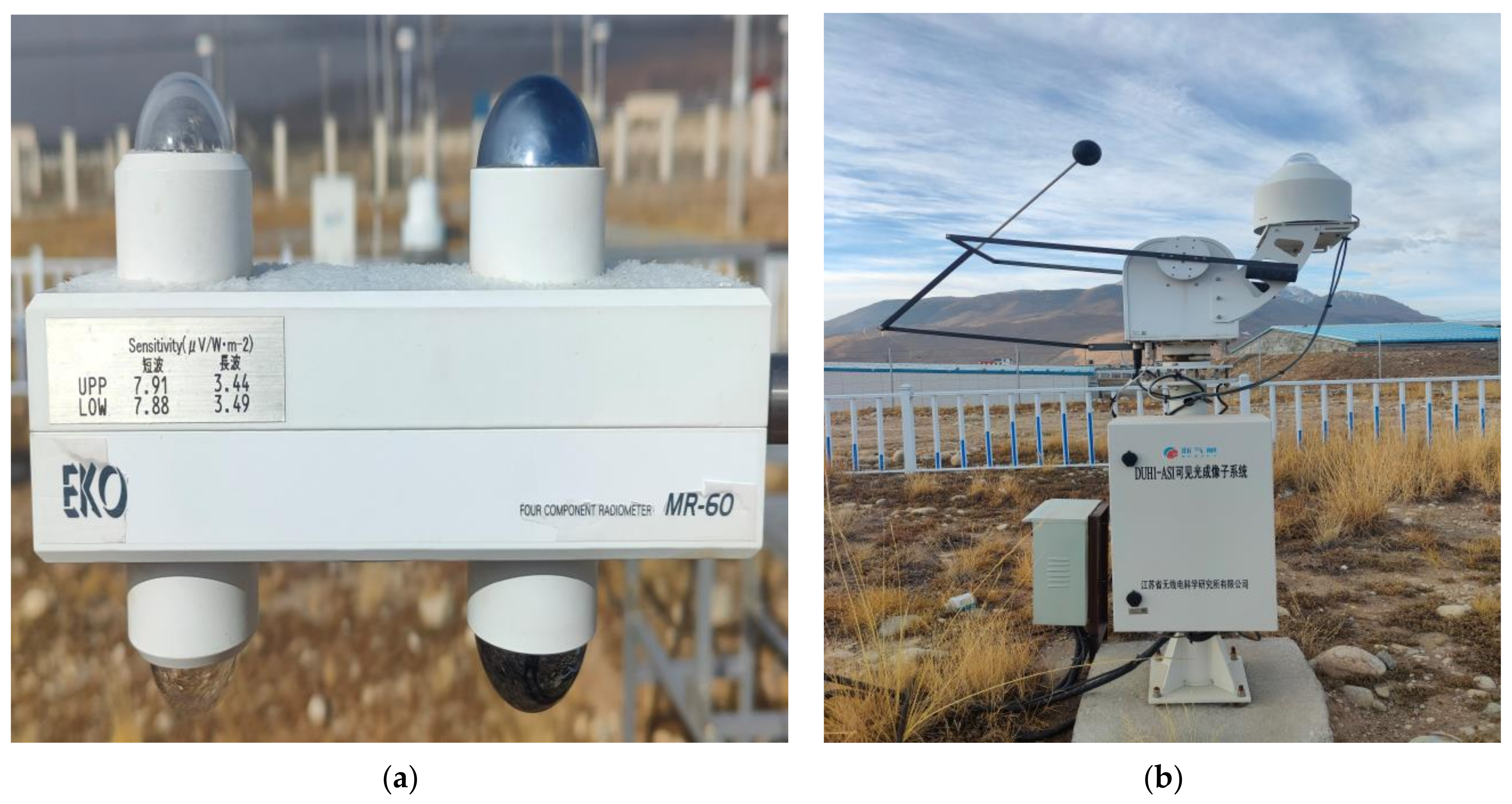
Figure 1. Data monitoring equipment. (a) Four-component radiometer; (b) Total Sky Imager.
Remotesensing 15 02340 g001
Figure 2. Cloud image processing flowchart. (a) The original cloud image; (b) cloud image pretreatment; (c) NRBR histogram; (d) cloud detection results (in this picture, the white area represents a cloud pixel, and the blue area represents a clear sky pixel).
Remotesensing 15 02340 g002
Figure 3. LSTM model architecture for predicting GHI. First, GHI quality control (singularity detection and resampling) is carried out, and cloud detection (NRBR) is carried out on ground-based cloud images. Then, the converted historical time series data of n-dimensional GHI and p-dimensional cloud cover are input to the LSTM input layer. After several hidden layers and a fully connected layer, the output layer outputs the predicted m-step GHI value.
Remotesensing 15 02340 g003
Figure 4. Number of model input features.
Remotesensing 15 02340 g004
Figure 5. Comparison of the model RMSE with different forecast horizons and step sizes. The red and blue broken lines show the RMSE amplitude change in the RF and LSTM models, respectively, when the prediction step size changes from 1 h to 10 min.
Remotesensing 15 02340 g005
Figure 6. NRMSE comparison of the model with and without cloud cover input variables. (a) RF model and prediction step size = 10 min; (b) LSTM model and prediction step size = 10 min; (c) RF model and prediction step size = 1 h; (d) LSTM model and prediction step size = 1 h. The red broken line is the amplitude change of the NRMSE of the model when the cloud cover input variable is added.
Remotesensing 15 02340 g006
Figure 7. The scatter plot of the predicted value (vertical axis) and measured value (horizontal axis) of GHI when the prediction step size is 10 min, the forecast horizon is 1 h, and the cloud cover is added as the input variable of the model. (a) RF model; (b) LSTM model. The red line is the fitting regression line of the predicted values and measured values, R-squared is the coefficient of determination, and the color on the color bar represents the frequency of each pair.
Remotesensing 15 02340 g007
Figure 8. Time series diagram of the measured irradiance value and predicted irradiance value (27 December 2020). (a) Forecast horizon = 1 h; (b) Forecast horizon = 5 h. The gray (measured) curve is the measured value, the dark red (RF-Cloud) and light red (RF-Cloudless) curves are the prediction curves with and without clouds as the RF model input variables. The dark blue (LSTM-Cloud) and light blue (LSTM-Cloudless) curves are the prediction curves with and without clouds as the LSTM model input variables.
Remotesensing 15 02340 g008
Figure 9. Scatter diagram of the measured GHI value and predicted GHI value (27 December 2020). (a) RF and forecast horizon = 1 h; (b) RF and forecast horizon = 5 h; (c) LSTM and forecast horizon = 1 h; (d) LSTM and forecast horizon = 5 h. The red and blue lines are the fitting regression lines of the predicted values and measured values with or without cloud cover as the model input variable, respectively, in which R-squared is the coefficient of determination.
Remotesensing 15 02340 g009
Table 1. Distribution of the cloud fraction in the Yangbajing area in 2020.
[0, 0.1)[0.1, 0.2)[0.2, 0.3)[0.3, 0.4)[0.4, 0.5)[0.5, 0.6)[0.6, 0.7)[0.7, 0.8)[0.8, 0.9)[0.9, 1]
Frequency388515109757747306726277999315872
Proportion (%)23.169.005.814.614.354.013.744.765.5535.00
Table 2. Monthly variation of the cloud fraction in the Yangbajing area in 2020.
JanuaryFebruaryMarchAprilMayJuneJulyAugustSeptemberOctoberNovemberDecember
Mean value0.560.490.640.720.790.660.780.630.550.120.290.28
Standard deviation0.410.390.370.320.310.310.280.360.360.190.390.38
Table 3. Number of model input features.
Forecast Horizon1 h2 h3 h4 h5 h6 h
GHIRF4476211
LSTM4519161087
Cloud fractionRF211111
LSTM1741512
Table 4. Comparison of the model RMSE with different forecast horizons and step sizes. The amplitude change reflects how much the RMSE changes when the prediction step size changes from 1 h to 10 min, and the best performance of the index is marked in bold font.
RFLSTM
Step Size =
1 h
(W/m2)
Step Size =
10 min
(W/m2)
Amplitude Change
(%)
Step Size =
1 h
(W/m2)
Step Size =
10 min
(W/m2)
Amplitude Change
(%)
1 h58.9531.8445.9960.1826.5655.87
2 h65.0343.9532.4273.1742.8941.38
3 h69.7654.9321.2686.0253.5837.71
4 h77.4662.9918.6890.5367.6825.24
5 h81.7271.2512.81101.0170.7929.92
6 h85.3579.856.44116.5880.1931.21
Table 5. NRMSE comparison of the model with and without cloud cover input variables. No cloud and add cloud represent the situation of no cloud cover input and cloud cover input, respectively, and the amplitude change reflects the change in the NRMSE after adding the cloud cover input variable. The best performance of the index is marked in bold font.
Step Size = 10 minStep Size = 1 h
RFLSTMRFLSTM
No Cloud (%)Add
Cloud (%)
Amplitude Change (%)No Cloud (%)Add
Cloud(%)
Amplitude Change (%)No Cloud (%)Add
Cloud (%)
Amplitude Change (%)No Cloud (%)Add
Cloud (%)
Amplitude Change (%)
1 h7.806.0722.186.815.0525.8415.5812.4620.0316.4312.7322.52
2 h9.058.426.969.908.2017.1715.6513.8011.8219.0915.4519.07
3 h11.2910.606.1112.3610.2716.9115.8914.926.1021.7018.5014.75
4 h13.9912.3611.6514.1313.117.2217.9116.617.2622.0819.1913.09
5 h16.4614.1613.9715.2713.879.1718.7717.576.3922.2921.344.26
6 h17.8515.9810.4816.6815.845.0419.4118.196.2925.1024.910.76
Disclaimer/Publisher’s Note: The statements, opinions and data contained in all publications are solely those of the individual author(s) and contributor(s) and not of MDPI and/or the editor(s). MDPI and/or the editor(s) disclaim responsibility for any injury to people or property resulting from any ideas, methods, instructions or products referred to in the content.