Article

Improving Solar Radiation Nowcasts by Blending Data-Driven, Satellite-Images-Based and All-Sky-Imagers-Based Models Using Machine Learning Techniques

by
Miguel López-Cuesta
1,
Ricardo Aler-Mur
2,
Inés María Galván-León
2,
Francisco Javier Rodríguez-Benítez
1 and
Antonio David Pozo-Vázquez
1,*
1
Andalusian Institute for Earth System Research IISTA-CEAMA, Department of Physics, University of Jaen, 23071 Jaen, Spain
2
EVANNAI Research Group, Department of Computing Science, University Carlos III, 28911 Madrid, Spain
*
Author to whom correspondence should be addressed.
Remote Sens. 2023, 15(9), 2328; https://doi.org/10.3390/rs15092328
Submission received: 17 February 2023 / Revised: 24 April 2023 / Accepted: 25 April 2023 / Published: 28 April 2023
(This article belongs to the Special Issue New Challenges in Solar Radiation, Modeling and Remote Sensing)

Abstract

:
Accurate solar radiation nowcasting models are critical for the integration of the increasing solar energy in power systems. This work explored the benefits obtained by the blending of four all-sky-imagers (ASI)-based models, two satellite-images-based models and a data-driven model. Two blending approaches (general and horizon) and two blending models (linear and random forest (RF)) were evaluated. The relative contribution of the different forecasting models in the blended-models-derived benefits was also explored. The study was conducted in Southern Spain; blending models provide one-minute resolution 90 min-ahead GHI and DNI forecasts. The results show that the general approach and the RF blending model present higher performance and provide enhanced forecasts. The improvement in rRMSE values obtained by model blending was up to 30% for GHI (40% for DNI), depending on the forecasting horizon. The greatest improvement was found at lead times between 15 and 30 min, and was negligible beyond 50 min. The results also show that blending models using only the data-driven model and the two satellite-images-based models (one using high resolution images and the other using low resolution images) perform similarly to blending models that used the ASI-based forecasts. Therefore, it was concluded that suitable model blending might prevent the use of expensive (and highly demanding, in terms of maintenance) ASI-based systems for point nowcasting.

1. Introduction

1.1. Importance of Solar Radiation Nowcasting

During the next decades, an enormous new photovoltaic (PV) solar power will be installed in many countries around the world [1]. This poses a formidable challenge regarding the grid integration of this new solar power. In power systems, reliable information of the solar generation available in the systems in the next minutes, hours and days is used to procure additional reserves or adjust the output of conventional generators, ensuring a balance between supply and demand. As a consequence, the development of accurate solar power forecasting methods has become a central area of research in solar energy [2,3,4].
Solar forecasting methods can be classified according to three forecasting horizons: nowcasting (up to 120 min ahead), short-term forecasting (up to 6 h ahead) and forecasting (up to days ahead) [5,6,7]. In the last years, the interest for the development of solar radiation forecasting methods has been moving from forecasting to nowcasting [8], fostered by the massive deployment of small-scale PV systems. Nowcasting is relevant for the management of residential-scale PV systems [9,10] and electricity systems with few interconnections as well as for electricity marketing and pricing [11].

1.2. Nowcasting Solar Radiation Methods

Nowcasting accounts for methods aimed at providing solar forecasts with very high spatial (order of meters) and temporal resolutions (order of minutes). The reference methods are based on the use of all sky imagers (ASIs) [12,13]. The forecasting horizon can reach about an hour [14,15]. ASI-based nowcasting has received notable attention in the last decade, but its reliability is relatively low [16,17,18]. Despite this, ASI-based solar nowcast has been successfully applied in several solar energy applications [19,20,21,22].
Short-term solar prediction reference methods are based on satellite imagery processing [23,24,25]. Satellite-images-based short-term forecasts have a typical spatial resolution of a few kilometers and a temporal resolution and latency of 15 min [26]. This makes the application of these methods less suitable for solar radiation nowcasting. Nevertheless, due to the availability of new satellite platforms, with enhanced spatial and temporal resolution, such as the Meteosat Third Generation (MTG) [27] and Himawari-8 [28], the interest in this method is increasing. Short-term forecasting has been successfully used for several solar energy applications [29,30,31,32,33].
As solar radiation measured datasets are progressively available, and given the rapid development of the machine learning (ML) methods, the use of these methods has become increasingly popular in solar forecasting. ML methods are applicable to all forecasting horizons, although they are mostly used for nowcasting studies. In addition, numerous works have used PV measurements, instead of solar radiation data (for a review see [34,35]). Yagli et al. [36] evaluated the performance of 68 different ML methods for hour-ahead solar forecasting. They report that the tree-based methods performed better.

1.3. Models Blending

There is a lack of research comparing solar nowcasts derived from the different methods. In addition, it is well known that when different forecasting models with similar accuracy are available, combined forecasts tend to provide enhanced forecasts [37]. By simply averaging the forecast, the bias and error variance can substantially be reduced in most cases. In the field of solar forecasting, some successful attempts have been made to combine data-driven satellite and NWP forecasts based on statistical techniques [38,39]. In a recent work, Nouri et al. [40] derived a statistical method to combine persistence (data-driven) and ASI-based solar radiation nowcasts in order to improve forecasts up to 20 min ahead.
The use of ML-based model blending approaches has been proposed as one of the most promising applications of artificial intelligence in earth sciences research [41]. In the review work of Zhou et al. [42], some important conclusions were obtained: (1) there is a severe lack of studies attempting to combine different models inputs using ML, and (2) regardless of the ML method used, the combination of different models’ inputs performs better than any single model.
ML-based model blending methods can follow different approaches. Pedro et al. [43] combined measured data and features extracted from ASI images to provide enhanced solar radiation forecasts 30 min ahead. They found significant forecasting skills and concluded that the use of ASI images is relevant for reducing the forecasting errors. Similar conclusions were reported by [44] with forecasts up to 15 min ahead. A second approach consists in the blending of different single ML-derived forecasting models, as in Heng et al. [11]. Following this approach, Fouilly et al. [45] built 11 different ML models to forecast solar radiation in the Mediterranean region. Then, they developed a methodology to select one of these models according to the meteorological conditions. The method provided enhanced hourly forecasts up to 6 h ahead. Chaman et al. [46] developed a set of different ML models to provide day-ahead global horizontal irradiance (GHI, hereinafter) forecasts, using the NWP forecast as input. Then, in a second step, an optimal blending of the models was obtained. The performance of the combined forecasts was found to be better than that of any single model.
Lastly, another approach consists in using ML methods to blend different solar forecasting models, based on different foundations. Following this approach, Wolff et al. [47] used support vector machine (SVM) models to combine irradiance measurements, satellite images and NWP solar forecasts. According to their results, the blended model provided enhanced hour-ahead solar PV forecasts. Similarly, Mazorra-Aguiar et al. [48] used ML to combine measured solar radiation, satellite images and NWP-based forecasts; the combined models provided enhanced GHI forecasts up to 6 h ahead. Qing and Niu [49] developed a blending model using different NWP models’ solar forecasts as input; they reported enhanced hourly day-ahead GHI forecasts. Dersch et al. [30] valuated an optimal combination of satellite and NWP forecasting models, obtaining improved Direct Normal Irradiance (DNI, hereinafter) forecasts. Finally, Huertas-Tato et al. [50] used SVMs methods to blend a data-driven model, a satellite-images-based model and a NWP model; their results showed that blending greatly outperformed the individual predictors.

1.4. Aim of This Paper

The aim of this work was to explore the benefits obtained by blending different solar radiation nowcasting models using ML techniques. The models (seven), which include data-driven, ASI and satellite-images-based models, provide one-minute time resolution and up to 90 min-ahead GHI and DNI forecasts. The study was conducted in an area located in Southern Spain using data corresponding to a set of days covering different cloudy sky conditions. The potential for improving forecast accuracy by model blending is worth exploring, as these models are based on different methods and provide similar performance. Two ML blending approaches were explored: horizon and general. For each approach, two different blending models were evaluated: random forest (RF) and linear. A set of experiments was conducted in order to evaluate (1) the performance of the horizon and general approaches and the RF and linear models, and (2) the relative contribution of the different forecasting models to the forecasting errors values reduction attained by the models blending. To the best of the authors’ knowledge, the blending of data-driven, ASI-based and satellite-images-based models for solar radiation nowcasting has not been addressed to date.
This work is organized as follows. Section 2 presents the dataset and the different nowcasting models. Section 3 describes the methods, presenting the different blending approaches and blending models, as well as the assessment procedure. The results are presented and discussed in Section 4. Finally, a summary is provided in Section 5.

2. Dataset and Models Input Description

2.1. Dataset and Study Region

This study was conducted in the area of the Abengoa Solar Platform of Solúcar (6.25W, 37.44N) (Figure 1), located near Seville, in Southwestern Spain. The datasets used in this study to build and evaluate the forecasting models include (1) ground measurements, (2) ASI images, and (3) low- and high-resolution satellite images. Within the platform (Figure 1), a set of three ASIs, a ceilometer and a radiometric station are located. The ASI-based forecasts were derived from images collected simultaneously by the three cameras and the ceilometer data. For satellite-images-based forecasts, Meteosat Second Generation (MSG) SEVIRI standard visible channels 1, 2 and HRV images, all with a latency of 15 min (full disk) are used. Images from these channels are available every 5 min (quick-scan mode) but with limited spatial coverage. Satellite raw images are transformed according to an azimuthal equidistant projection in order to have a spatial resolution of 5 × 5 km (channels 1 and 2) and 1 × 1 km for the HRV channel images. Data from the radiometric station were used for deriving a data-driven reference model and for validation purposes. This radiometric station includes an Eppley Black and White pyranometer and an Eppley NIP pyrheliometer. Raw data were quality-check analyzed according to the procedures defined by Long and Dutton [51]. In addition, raw data greater than 75° of solar zenith angle were discarded by this procedure.
Finally, a dataset collected along 43 days, from June to October 2015, was used in this work. The dataset is composed mostly of cloudy sky conditions (altocumulus, cirrocumulus, cumulus, stratocumulus and multicloud). Therefore, the artificial improvement of the forecasting skill obtained by clear sky conditions was limited. In order to reach the longest possible forecasting horizon, only cases where the clouds moved toward the northeast direction were considered. Note that the validation station is located northeast of the ASI positions (Figure 1).

2.2. Models Input Description

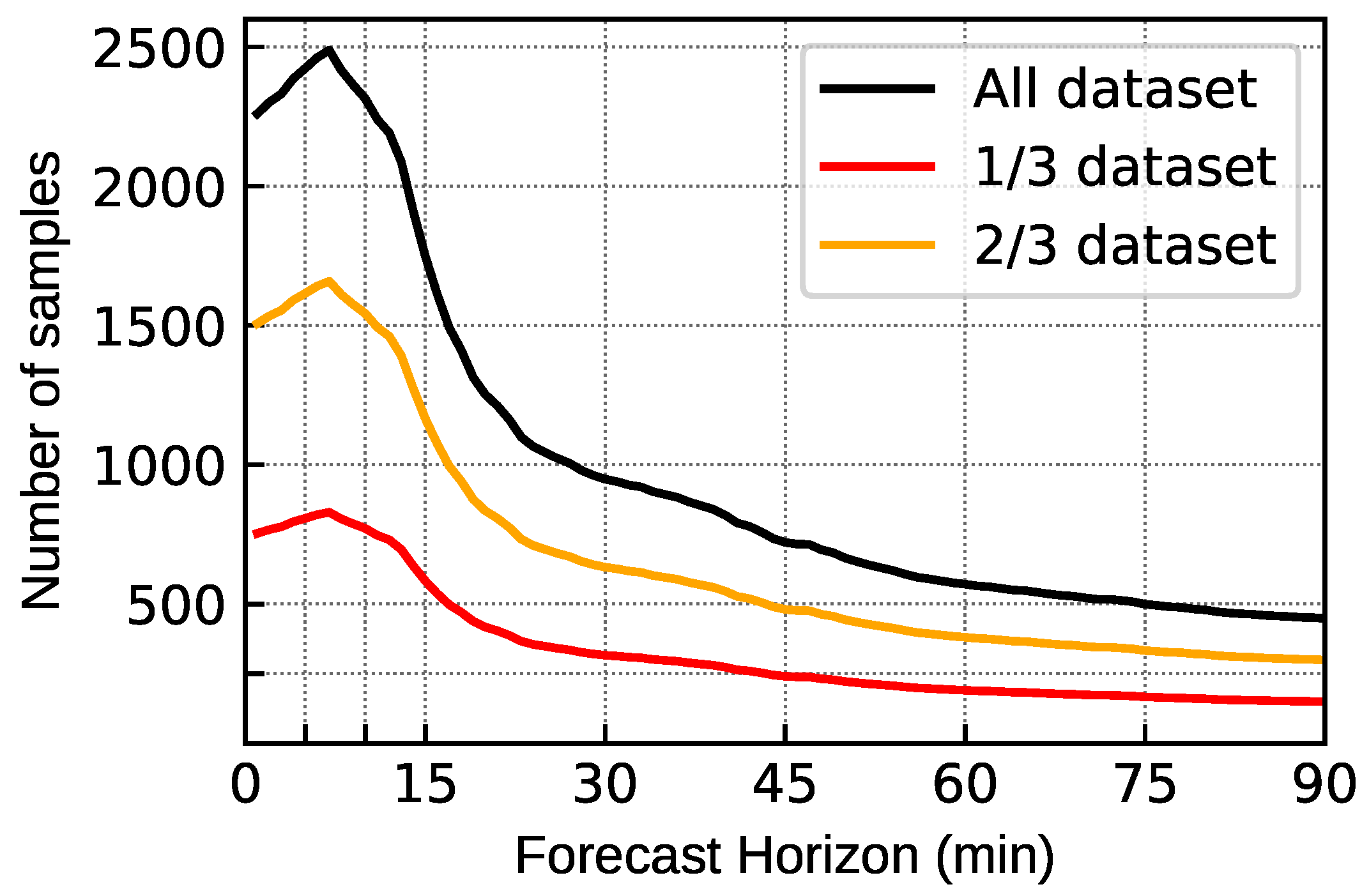
A set of seven nowcasting models (hereinafter input models) was used in this study; the models and their main characteristics are listed in Table 1. The models were presented and validated in [14]. For each model, a set of GHI and DNI nowcasts are available, with a time resolution of one minute and a forecasting horizon up to 90 min. Only samples (forecasts) available for every ASI and satellite model at a given horizon were considered. As observed in Figure 2, the number of samples available decreases with the forecasting horizon. The relatively low number of samples for longer horizons is due to the limited viewing area of the sky covered by ASIs. Only in certain cases (quasi-stationary clouds and/or high medium/high clouds) do the ASIs provide 90 min-ahead nowcasts. A total of 88,650 valid forecasts (for every model) were used to build and evaluate the different ML blending models.
Four input models were derived from the three ASI located in the study area. ASI-based forecasts are obtained by processing two consecutive images (at one-minute time step). The processing encompasses several steps. Firstly, a georeferentiation procedure is applied with the aim of cropping a reliable portion of the distortion-corrected sky image and deriving the size estimation of each pixel (length/pixel ratio). To this end, the cloud base height derived by the ceilometer is used. Secondly, an algorithm is used to determine, for each pixel of the image, whether the pixel corresponds to a cloud or a portion of clear sky, or whether it is a null-value pixel. In this work, the hybrid thresholding algorithm (HYTA) described in [52] was used. In the third step, the so-called cloud motion vectors (CMVs) are estimated using the DeepFlow algorithm [53]. These CMVs represent the apparent cloud displacement by comparing two consecutive images. In a further step, the images are advected into the future, at the forecasting horizon of interest, using the CMVs (CMVs are selected in a specific direction in order to increase the maximum forecasting horizon). Then, each image is inspected in order to determine the characteristics of the sky around the validation station. From this information, finally, DNI and GHI forecasts can be derived with the help of a clear sky model; in this work, the ESRA [54] model was used. DNI forecasts are directly derived as the product of the clear-sky DNI estimation and 1-CF, where CF is the cloud fraction value. This CF value is computed as the ratio of the numbers of cloudy pixels to the total amount of valid pixels in a circle containing the sun. The GHI forecasts are derived following the procedure proposed by [12]. The method firstly computed the clearness index (ratio between GHI measured and GHI of clear sky called K c , hereinafter) from the GHI measured values 30 min before the forecasts were issued. Then, using a K-means clustering algorithm, two representative K c values were obtained. If the CF value was greater/(lower) than 0.4, the lowest/(highest) K c value was selected. Finally, the GHI forecasts were computed as the product of the selected K c and the corresponding clear-sky GHI estimation. Based on this procedure, three ASI-based forecasting models inputs were obtained (hereinafter ASI-1, ASI-2 and ASI-3). The fourth model input (hereinafter ASI-mean) was obtained by averaging the ASI-1, ASI-2 and ASI-3 models forecasts at each time step.
Two satellite-images-based forecasting input models were used in the study. The models used images corresponding to several channels of Meteosat Second Generation (MSG) geostationary satellites [55], operated by the European Organization for the Exploitation of Meteorological Satellites (EUMETSAT). The procedure to derive the GHI and DNI forecasts from the satellite images was similar to the procedure used in the ASI-based forecasts. Firstly, the so-called cloud index (CI) image was computed from the satellite images. The CI image represents the state of the sky at each pixel using a number whose value ranges from 0 (cloudless pixel) to 1 (overcast pixels). In this study, the Heliosat method [56] was used to derive the CI. In a second step, two consecutive CI images were compared, using two algorithms to derive the CMVs: the OpenPIV [57] algorithm for the low-resolution MSG images, and the deep flow approach for the high-resolution MSG images. In addition, the streamlines of the cloud movements were computed from the CMVs field following [58]. The streamlines account for the trajectory and velocity of the clouds displacement. Once the streamline has been calculated, the pixels above the validation station at each time step can be identified in the satellite image. Using these streamlines, the satellite models forecasts temporal resolution and latency were increased to one minute, in order to match the characteristics of the ASI-based forecasts [14]. Finally, a clear-sky model was used to derive the GHI and DNI forecasts. Following this methodology, the two satellite-images-based models used in this study were obtained. The first one (hereinafter Sat-LR) uses the low-resolution MSG channels (channels 1 and 2) to derive the CI images and has a spatial resolution of 5 km. The second one (hereinafter Sat-HR) uses the high-resolution MSG channel, which has a 1 km spatial resolution.
Lastly, a data-driven model was used in this study, based on the GHI and DNI data measured at the validation station. This model (hereinafter Smart-Persistence) uses the ratio between the radiation measured at the time the forecast is issued and the corresponding clear sky value. Then, at each forecasting horizon, the forecast is computed as the product of this ratio and the corresponding clear-sky value (Equation (1)):
I ( t ) = I 0 I c l e a r s k y · I c l e a r s k y ( t ) ,
where I 0 is the measured radiation value at the time the forecast is issued, I c l e a r s k y is the corresponding clear-sky estimate, and I c l e a r s k y ( t ) is the clear-sky irradiance estimate at forecasting horizon t. This approach ensures that the Smart-Persistence model error at lead 0 min (time at which the forecasts are issued, t = 0) is 0. Other persistence models use the measurements of the previous instant (t = −1). The temporal resolution of Smart-Persistence is 1 min and I stands for both the GHI and DNI. As in the case of ASI-based and satellite-based forecast models, the ESRA clear-sky model was used. Smart-Persistence models, while basic, tend to provide reliable forecasts for the first few minutes of lead time. These models are used for benchmarking more complex forecasting models.

3. Methods

This section describes the methodology followed to obtain the blending models. Firstly, the two different blending approaches used in this study (general and by horizons) are explained. Secondly, the ML techniques used (RF and linear) are described. Thirdly, the evaluation procedure is presented. Finally, the different experiments conducted and evaluated are presented.

3.1. Horizon and General Approaches

The blending approach consists in developing ML models using as input the irradiance forecasts of the seven models M 1 , M 2 , …, M 7 described in the previous section. The blending ML model provides at each time point (t) a new irradiance forecast (I) for different forecasting horizons (h). This prediction is provided at 1 min time steps, constituting the ML combination of the seven M i irradiance prediction models. In this work, 90 forecasting horizons with 1 minute steps were considered. Depending on the structure used to train the ML blending models, two different approaches can be considered: the horizon approach and the general approach. In the horizon approach, a model was constructed for each forecasting horizon using training data from that horizon only. In the general approach, a single model was constructed and trained with all the forecasting horizons. These two approaches are described in Appendix A, and more information can be obtained in [50].

3.2. Machine Learning Algorithms

The blending ML models described in Section 3.1 and Appendix A were estimated using a linear approximation and RF. The linear approximation consisted in a linear combination of the model inputs and RF is the non-linear ML method used in this work. Both methods are explained in detail in Appendix B.

3.3. Model Blending Experiments

A set of experiments was conducted, involving different sets of the seven models’ inputs described in Section 2.2 (Table 1), and using the two blending approaches and the two blending models. Figure 3 shows a outline of the procedure. The experiments were aimed, firstly, at determining the best performing blending approach (horizon vs. general) and blending model (RF vs. linear) and, secondly, at evaluating the relative importance of the different input models in the blending models’ performance. Table 2 lists the sets of inputs models involved in the experiments, using acronyms for the sake of conciseness. All the sets included the Smart-Persistence model. The set acronyms with the word “Sat” included one of the satellite-images-based input models, or both. The sets with the word “ASI” included some/all of the ASI-based input models. In experiments using only an ASI-based model, the ASI-1 was selected. No differences were found using ASI-2 or ASI-3. Note that the three ASIs are located relatively close to each other and are the exact same instrument model.
Based on the sets of models inputs listed in Table 2, and following the procedure showed in Figure 3, different studies were conducted. In the first study, a set of experiments was carried out using, for each set listed in Table 2, the two blending approaches (horizon and general) and the two blending models (linear and RF) (i.e., 36 experiments for the GHI and DNI). This study was aimed at determining the best performing blending approach (horizon vs. general) and blending model (linear vs. RF). The results from this study are presented in Section 4.1; only one of the blending approaches and one of the blending algorithms were selected and further considered in the study.
In the second study, a thorough analysis was conducted to determine the importance of the different input models in the model blending results. Notably, in this study, the relative contribution of the ASI-based and satellite-based models to reduce the forecasts errors was assessed. The results of this analysis are presented in Section 4.2.
In a third study (Section 4.3), the performance of the different blending models as a function of the forecasting horizon was assessed.
Finally, as a method to evaluate the real benefit attained by the ML blending procedures assessed in this work, the results of the best performing blending experiments were compared using two models. The first model was obtained by simply averaging all the models inputs listed in Table 1 (hereinafter the average model). Note that this is a trivial model blending approach. The second model is a more stringent reference model, constructed based on the best forecast for each horizon as derived from all the input models (hereinafter the optimal model). Note that this model cannot be used in operational forecasting, since the best-performing forecasts at each horizon are unknown beforehand. Nevertheless, it can be used as a stringent reference to compare the performance of the model blending approaches considered in this work. The results of this assessment are presented in Section 4.4.

3.4. Evaluation Procedure

3.4.1. Training and Evaluation Datasets

The model-blending procedure requires a training and validation dataset. In this work, the dataset was divided into two randomly selected groups: 2/3 of the dataset was used for training the models and the other 1/3 for an independent validation. In order to conduct a fair validation, the dataset was firstly divided in 2 h packages. Then, training and validation datasets were filled by randomly selecting the 2 h packages. This reduced the eventual influence on the models performance of solar radiation time series autocorrelation.

3.4.2. Evaluation Metrics

In this work, two metrics were used: the relative root mean squared error (rRMSE, Equation (2)) and the forecast skill (FS) in terms of RMSE of the Smart-Persistence method (Equation (3)):
rRMSE ( t ) = 1 N i = 1 N ( I forecast ( t , i ) I measured ( t , i ) ) 2 1 N i = 1 N I measured ( t , i ) ,
FS RMSE ( t ) = 1 RMSE forecast ( t ) RMSE SmartPersistence ( t ) ,
where N is the total number of samples, I corresponds to GHI or DNI, and RMSE SmartPersistence is the RMSE corresponding to the Smart-Persistence forecast model.

3.4.3. Feature Importance

One of the advantages of the RF blending model is that a parameter called feature importance can be easily calculated. This parameter provides information about the importance of the input variables used to build the RF model. In this work, the mean decrease impurity (MDI) was used [59,60]. This value is computed by the RF method in the scikit-learn Python library [61] by adding the mean squared error decrease provided by a particular variable every time the variable is used in a node in the tree for splitting the training samples (as was explained in Section 3.2). The mean squared error reduction is weighted by the number of samples split by the node where the variable is used. This value is averaged across all trees in the ensemble. Therefore, in this study, the MDI value provides information about the importance of the different models inputs in the forecasting error reduction attained by the RF model blending. It is important to remark that MDI measures the importance of features, not in an absolute way, but relative to the model that uses them. Thus, a feature with a low MDI is not necessarily irrelevant for the task at hand, as it may rather mean that the model does not find that feature useful, probably because other features that provide similar or better information are used in its place. This insight is particularly important for trees, as they choose features in order, from the root node to the leaves. Therefore, once some features are selected for the top nodes in the tree, new variables are chosen (with preference to others) only if they provide new information, in addition to the information provided by the already selected variables.

4. Results and Discussion

4.1. Assessment of Blending Approaches And Models

In this section, the overall performance of the different blending approaches (Section 3.1) and blending models (Section 3.2) is assessed. To this end, a set of experiments (Section 3.3), alternately using the general and horizon blending approaches and the linear and RF blending models, is evaluated (Figure 3). Table 3 lists the validation rRMSE values derived from these experiments for both GHI and DNI forecasts. The rRMSE values were derived considering all the forecasts (88,650 samples), regardless of their forecasting horizon.
The results in Table 3 clearly indicate, firstly, that the general approach provides more accurate forecasts than the horizon approach. This is observed for both GHI and DNI, and regardless of the blending model. Secondly, Table 3 shows a superior performance of the RF blending model for experiments using the general approach. These experiments obtained rRMSE values about one third lower than those obtained by the linear model. For the experiments using the linear model, almost no differences were observed between the experiments using the general and horizon approaches. It was detected that DNI forecasting error values tended to be about twice the corresponding GHI counterpart value. Finally, given a blending approach and blending model, differences in the performance of the different experiments tended to be relatively low.
To sum up, the main conclusions that can be derived from the analysis of the results in Table 3 is that the general approach using the RF model (hereinafter the General-RF experiments) provides enhanced forecasts. This was observed for all the experiments and for both GHI and DNI, with Sats & ASI being the best-performing experiments (rRMSE 21.8%) for GHI and Sats (rRMSE 42.2%) for DNI forecasts. Additional analyses (not shown) were conducted using other evaluation scores (RMSE, MAE and rMAE), and the same conclusions were derived. This confirms the reliability of the models’ performance differences presented in Table 3.
To date, few works have compared general and horizon approaches in the field of solar forecasting. In a previous work [50], these approaches were compared for intra-day solar forecast; the general approach was also found to perform better. Chaman et al. [46] compared the performance of models aimed at providing day-ahead forecasts for all the sunny hours of the day and models specifically trained for each hour of the day. Similar to the results obtained from this study, the forecasting performance of one-for-all-hour models was found to be better than that of the hourly models. The rationale behind these results could be related to the number of samples available for each approach. While the general approach procedure uses all of the available samples, the horizon approach uses a much more limited number of samples at each forecasting horizon. This may limit the performance of the horizon approach. On the other hand, autocorrelation of the solar forecasts, and their forecasting errors, may help in reducing the forecast errors when using the general approach. Regarding the blending model, the superior performance of the RF approach was previously reported. For instance, Fouilly et al. [45] evaluated 11 different ML models for hour-ahead solar forecasts in the Mediterranean region. The RF model was found to provide a superior performance under highly variable weather conditions (i.e., the most stringent). Non-linear blending models were also found to be superior [46]. In general, nonlinear ML methods, and especially tree-based methods, have been reported to outperform other approaches regarding solar radiation forecasting [36]. The rationale behind these results may be related to the complex and nonlinear dependencies of solar radiation, which are better accounted for by tree methods. Given the previous results, only the General-RF experiments results are considered and analyzed in the following sections.

4.2. Assessment of the Importance of the Models Inputs

The results from the previous sections reveal that the experiments using the general approach and RF model provide the best performance. In this section, the relative importance of the different model inputs in this experiments is further assessed. To this end, firstly, the results from different experiments using different combinations of model inputs were compared and, secondly, the “feature importance parameter” of the RF blending model procedure was analyzed.
The results in Table 3 for GHI (first row) reveal that the General-RF experiments using the two satellite and the ASIs-based model inputs, i.e., Sats & ASI-mean, Sats & ASI and Sats & ASIs experiments, provide enhanced forecasts, with the rRMSEs values associated with these experiments being very similar (21.9, 21.8 and 22.8%, respectively). Note that the use of more than one ASI model does not improve the results. Results also reveals that the experiment that just included both satellite model inputs (Sats) provided a similar performance (22.9%) with respect to the experiment that used both satellites and, additionally, some ASI-based model as input. Lastly, the experiments that only used one of the two satellite models and the ASI model as inputs (Sat-LR & ASI and Sat-HR & ASI) provided considerably higher forecasting errors (27.1% and 28.1%, respectively). Similar conclusions can be derived for the DNI (fifth row in Table 3). Finally, it is worth noting the low performance, both for GHI and DNI, of the experiments that included the Smart-Persistence model and only one of the image-based models (ASI, Sat-LR and Sat-HR).
From this analysis, several conclusions can be derived. Firstly, regarding the use of the ASI-based models, no significant differences were observed when using only one camera model input (any of the three available) or using the mean of the three models. Similar results, regarding the importance of the ASI input in blending models, were found in previous studies [43,44]. Secondly, and more important, the blending models that used the two satellite model inputs (Sats), with no ASI model input, provided very competitive forecasts, performing similarly to those blending experiments that used as input some of the ASI-based models too. Therefore, the use of the two satellite models as inputs is always necessary to derive accurate forecasts, while the use of the ASI-based models can be avoided.
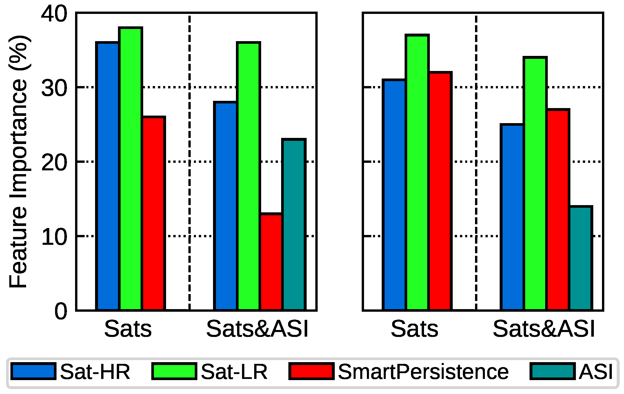
In order to explore further the relative importance of the different input models in the blending experiments results, an additional analysis was conducted. Notably, the feature importance (explained in Section 3.4.3) in the General-RF blending model procedure was analyzed for two experiments: Sats and Sats & ASI (best-performing ones). The analysis of these two experiments allowed evaluating the relative importance of the Smart-Persistence, Sat-LR, Sat-HR and ASI input models in the model blending results. The results of this analysis are presented in Figure 4.
Regarding GHI (Figure 4 left), the most relevant input model for the Sats & ASI experiment (the best performing one) was Sat-LR (36% importance), followed by Sat-HR (28%) and ASI model (23%). The least important model was the Smart-Persistence model (13%). The results for the Sats experiment reveal that, again, the Sat-LR input model was the most relevant (38%). The second-most-important model was Sat-HR (36%), while Smart-Persistence was the least-important model (26%). Based on the fact that the performance of the two blending experiments (Sats & ASI and Sats) was very similar (Table 3, first row), some conclusions can be derived from the above results. Firstly, the most important model input for all the experiments was the low-resolution satellite (Sat-LR) model. Sat-LR is more important that the Sat-HR, even its coarser resolution. This could be related to the reliability of the solar radiation estimates: while the Sat-LR uses information from two channels, the Sat-HR uses information from only one [14,62]. It has been shown that solar radiation estimates and forecasts derived from the low resolution images outperformed the estimates derived from the high-resolution ones under cloudy conditions [14,63]. Nevertheless, the contribution of the Sat-HR model is critical, and the performance of the experiments that do not use this model is poor. This indicates that the high-resolution images provide valuable information not contained in the low-resolution images, probably related to the spatial variability of the solar radiation, in the blending procedure. Secondly, since the feature importance of the Sat-LR model input was similar in the Sats & ASI and Sats experiments (36% and 38%, respectively), it can be concluded that the forecasting information derived from the ASI-based model can be extracted, based on the blending procedure, also from the Smart-Persistence and the Sat-HR model. Note that the feature importance of the persistence model increased from 13% in the Sats & ASI experiment to 26% in the Sats experiment. Similarly, the importance of the Sat-HR increased from 28% to 36%. Therefore, the relative contribution of Smart-Persistence and Sat-HR seems to be similar in providing the ASI-derived forecasting information.
The results differ for DNI (Figure 4 right). The most relevant input model for the Sats & ASI experiment was the Sat-LR, as in the case of GHI (34% importance). However, the second-most-important model was the Smart-Persistence model (27%), and the third-most-important model was Sat-HR (25%). The least-important input model was the ASI model (14%). The results for the Sats experiment (the best-performing one) reveal that, again, the Sat-LR satellite input model was the most relevant (37%). The other two input models, i.e., persistence and Sat-HR, proved to be of very similar importance (32% and 31%, respectively). As for GHI, it can be concluded that the forecasting information derived from the ASI-based model can be extracted, based on the blending procedure, from the Smart-Persistence and the Sat-HR input models. The main difference between the GHI and DNI results is the enhanced role of the Smart-Persistence input model and the diminished role of the ASI-based input model for the DNI forecasts compared to the GHI ones.
Overall, the results from this section show that the inclusion in the blending model of ASI-based and satellite-based forecasts provides enhanced GHI and DNI. However, the results also show that the blending of only the data-driven model and the two satellite-images-based models (one using high-resolution images and the other using low-resolution ones) performs similarly to those blended models that used the ASI-based forecasts. Therefore, the use of ASI-based forecasting systems, which are expensive and highly demanding in terms of maintenance, can be avoided. As was reported by Samu et al. [8], the use of ASI-based forecasts is nowadays seen as challenging by potential users in energy applications, due to both the cost of the systems and their relatively low performance.

4.3. Forecasting Horizon Dependency

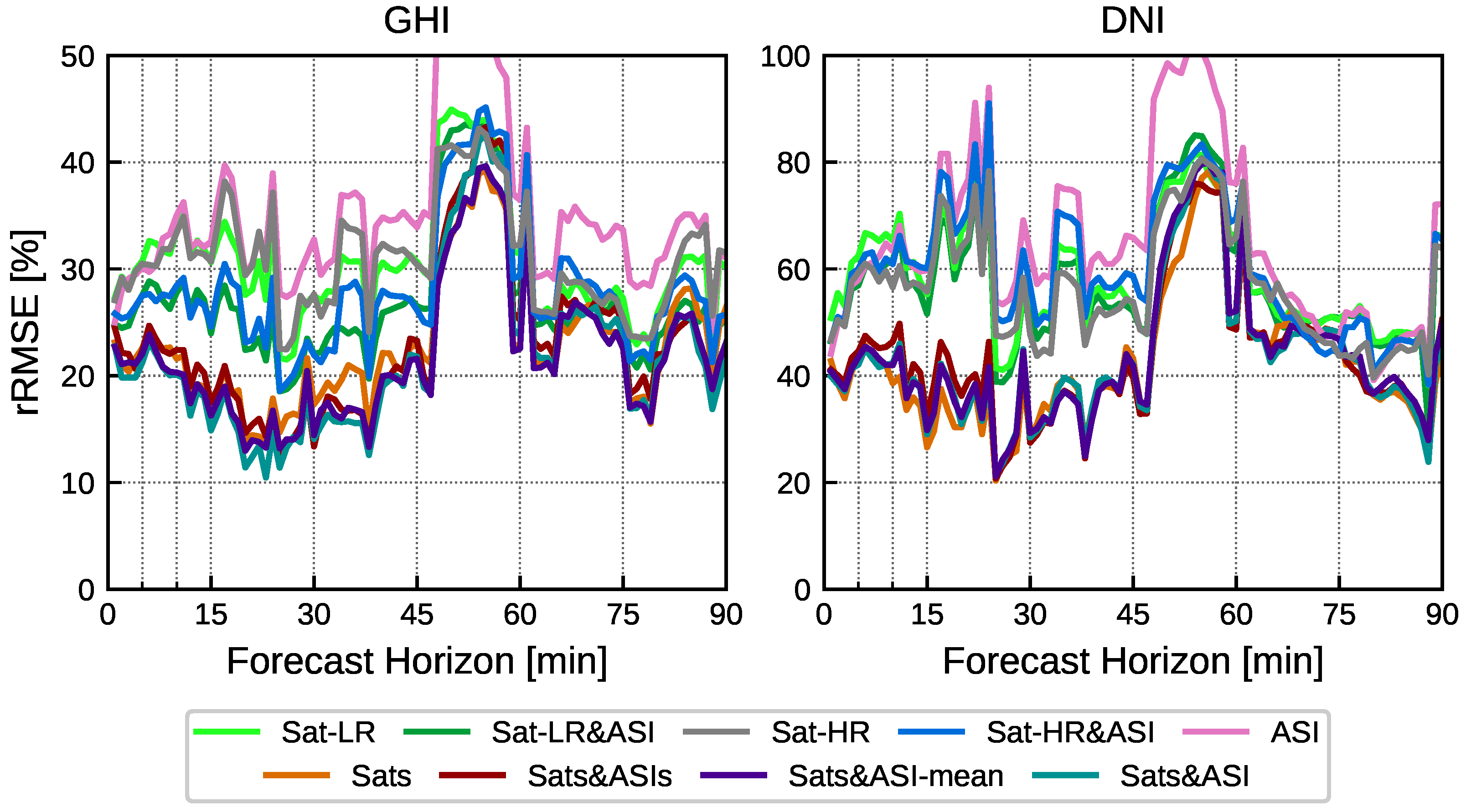
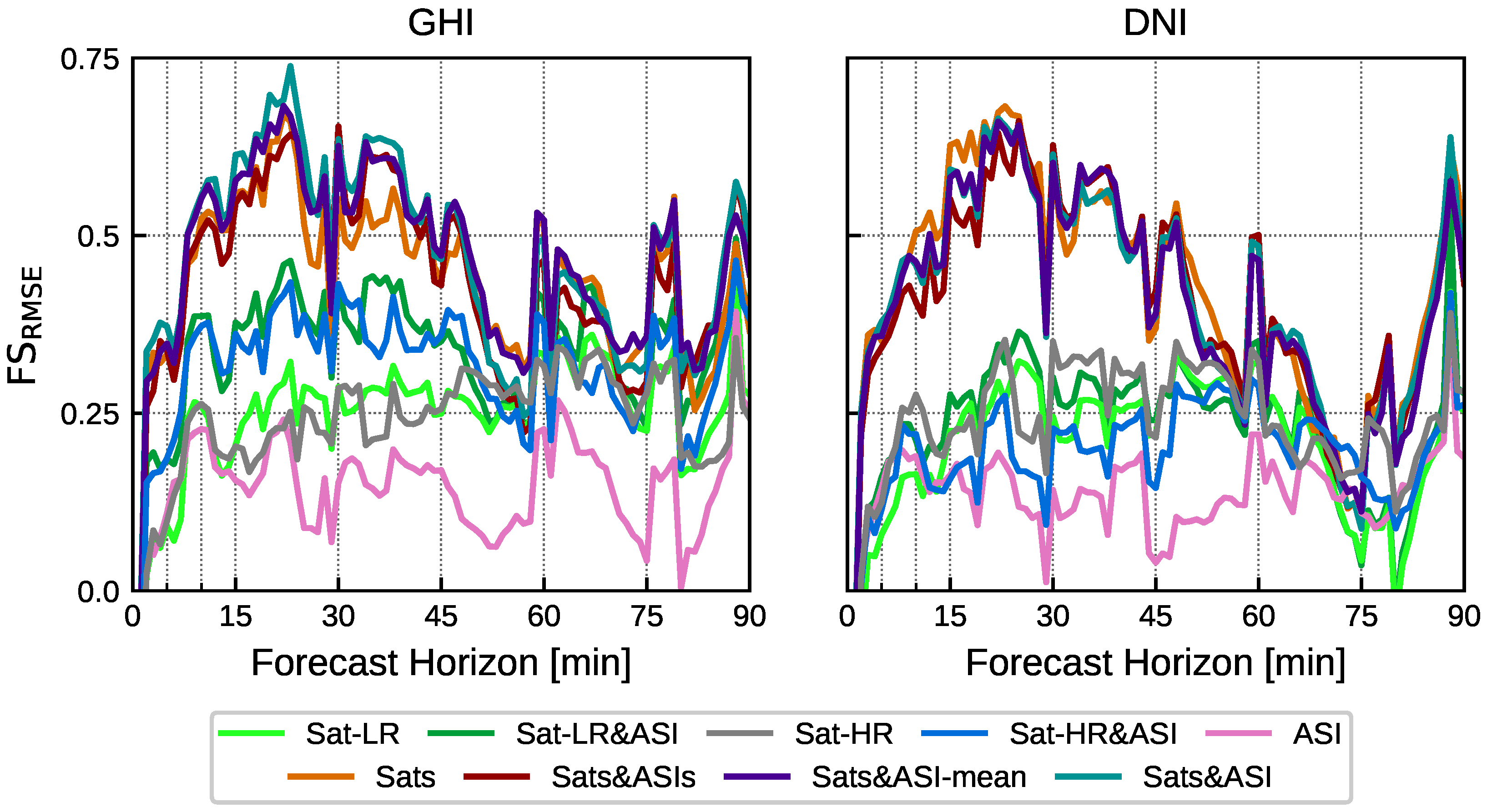
In the previous section, the overall performance of the different experiments was assessed. In this section, the performance of the experiments as a function of the forecasting horizon is assessed. A study of the feature importance as a function of the forecasting horizon cannot be conducted for the general approach. Figure 5 and Figure 6 show, respectively, the rRMSE and FS values for the nine experiments conducted using the General-RF blending model, whose overall results are listed in Table 3. The values are represented as a function of the forecasting horizon.
The analysis of both figures reveals three important results. Firstly, the poor performance of the experiments that include just one image-based model along the whole forecasting window is evident, as may be expected from the results analyzed in the previous sections. Secondly, the differences in the experiments performance are mostly limited to forecasting horizons below 45 min. Therefore, the differences in model blending performance listed in Table 3 are mainly related to the 1-45 min forecasting horizon range. This is observed for both the GHI and DNI forecasts. Lastly, the three experiments that include both satellites and the ASI input models (Sats & ASIs, Sats & ASI and Sats & ASI-mean) provide slightly enhanced forecasts along 1–45 min (Figure 6). On the other hand, the two experiments that used just one of the satellite-derived forecasts (Sat-LR & ASI or Sat-HR & ASI) provided a poor performance at lead time below 45 min, particularly for DNI. The performance of the Sats model is particularly outstanding since, along the whole forecasting period, it provided competitive forecasts for both GHI and DNI. In addition, it is the best-performing model at some lead times for DNI. Maximum differences in the experiments performance occurred at lead times between 10 and 30 min, and they are considerably higher for the DNI forecasts. For instance, for GHI (Figure 5 left), differences in the rRMSE values between models in this forecasting window were up to about 15% in absolute terms (15% vs. 30%, i.e., a 100% relative difference). In the case of DNI (Figure 5 right) differences reached 40% (40 vs. 80%, i.e., a 100% relative difference). Differences in FS values for GHI (Figure 6 left) reached 0.25 in this time window (0.5 vs. 0.75), while for DNI (Figure 6 right), differences close to 0.5 were observed. Therefore, this forecasting window is where the model blending provides the highest added value.
Figure 6 reveals some additional characteristics of the experiments’ performance. Firstly, the skill of all the experiments is considerably low at the beginning of the forecasting window, at lead times between 1 and 5 min. This was observed for all the experiments and both GHI and DNI. This means that the persistence model plays a central role in the blended model at these horizons. On the other hand, the maximum FS values were observed at around the 20 min forecasting horizon for all the experiments, being slightly higher for the GHI forecasts. This indicates that the satellite images and ASI-based models provide the most relevant contribution to the blending around this forecasting time. This could be related to the spatial information provided by these images that contains information about the spatial variability of the clouds and, therefore, of the solar radiation in the next few minutes. Beyond 20 min, its seems that the value of this spatial information is reduced, probably due to the “frozen clouds” assumption of the image-based forecast models. That is, cloud shapes evolve and change over time due to thermodynamic processes. It seems that beyond 20 min, on average, the clouds change so dramatically that information collected 20 min earlier begins to lose meaning, adding little to the information provided by the measurements.
An additional feature observed in Figure 6 is that the skill of the Sat-HR & ASI and Sat-LR & ASI experiments for DNI was considerably lower than that of the corresponding GHI experiments along the whole forecasting period. As was observed, the FS values of these two experiments are hardly ever greater than 0.25 for DNI, while for GHI, FS is above this value along almost the whole forecasting window. This may be related to the very low skill of the ASI-based models for DNI forecasts compared to GHI forecasts [14]. DNI nowcasting is much more challenging that GHI nowcasting, and ASI-based models provide scarce “added value” to the Smart-Persistence model for DNI point nowcasting. Lastly, and most importantly, Figure 5 and Figure 6 reveal, as was previously highlighted, that the Sats experiments performance was similar to that of the experiments that used both satellites combined with any of the ASI-derived input models. This is true for the whole forecasting horizon and for both GHI and DNI.
The results are particularly outstanding at the first lead times (from 1 to 5 min). In this forecasting window, the experiments Sat-HR, Sat-LR, ASI, Sat-HR & ASI and Sat-LR & ASI, which do not include both satellite models, provided almost no skill for DNI. Nevertheless, the Sats provided a FS value similar to that of the best experiments (Sats & ASIs, Sats & ASI-mean and Sats & ASI), which includes some of the ASI models as input. Therefore, the model blending procedure was particularly successful in the blending of the two satellite model inputs and for DNI.

4.4. Model Blending Comparison

From the previous analyses, it is clear that General-RF is the best-performing model and Sats & ASI and Sats are the best combination of the input models, for GHI and DNI forecasts, respectively. These blending models were evaluated based on the relative performance of different model inputs combinations and using the persistence model as reference (FS). A final analysis was conducted in order to assess the real “added value” of the ML-based blending model obtained in this work. To this end, the performance of these two models was compared against a trivial blending approach (average model), and against a stringent reference model based on the best of all single input models (optimal model), both described in Section 3.3.
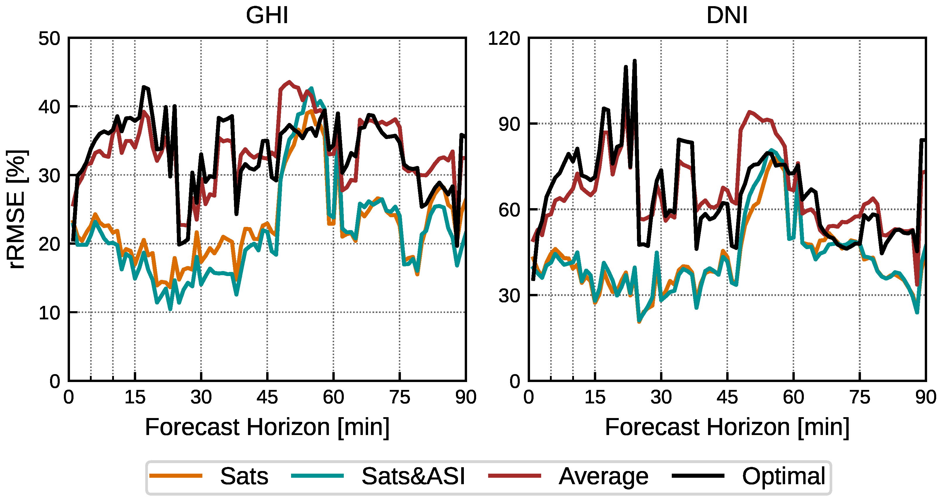
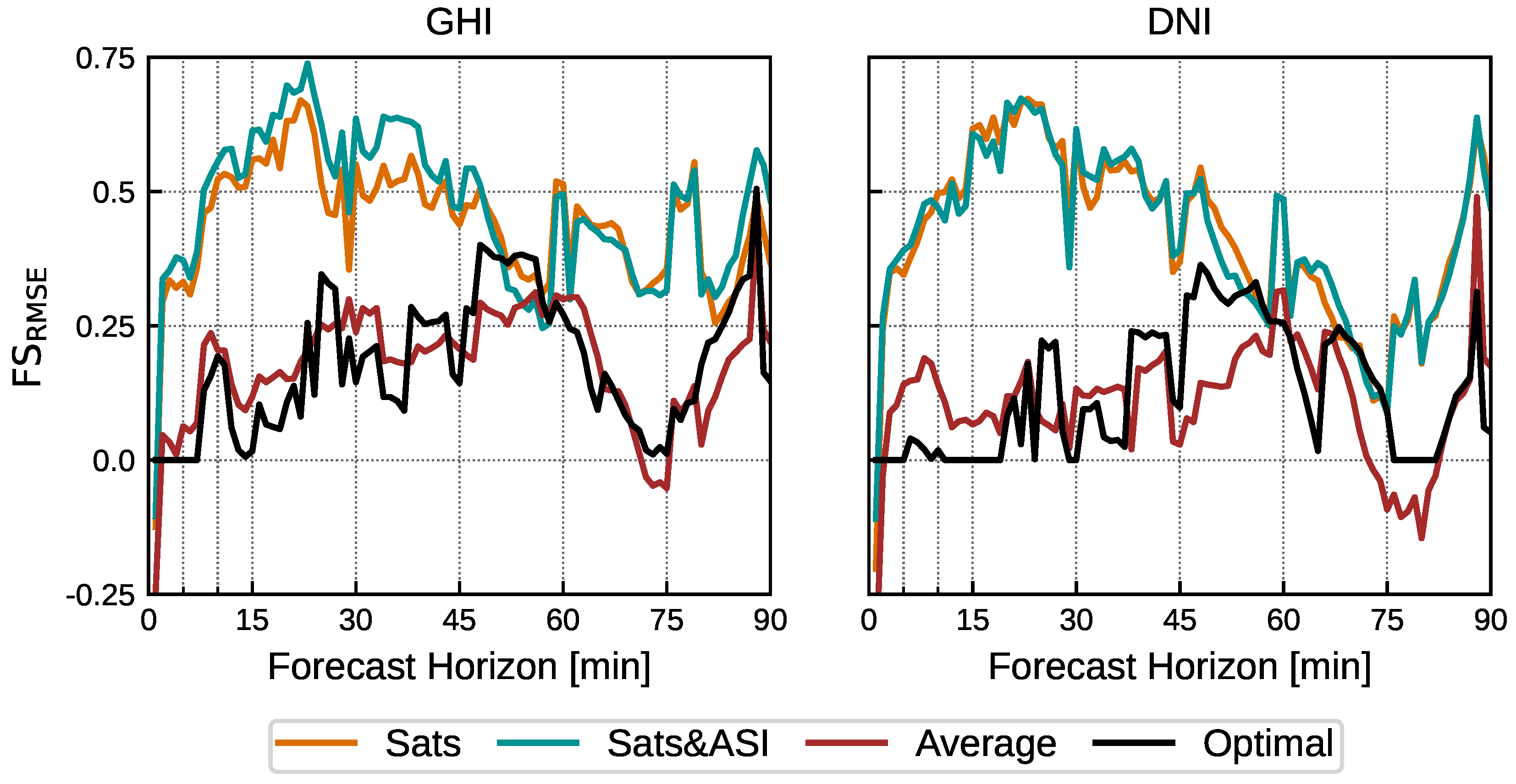
Figure 7 and Figure 8 show, respectively, the rRMSE and FS for GHI and DNI for these models. For the GHI, the Sasts & ASI model outperformed both the average and optimal models for almost all the forecasting horizons. In the case of DNI, the Sats model also outperformed both the average and optimal models.
Regarding the rRMSE values (Figure 7), maximum differences were observed in the forecasting period between 15 and 30 min; in this time window, differences of about 30% (15% vs. 45%) for GHI and 40% (80% vs. 40%) for DNI were obtained. Minimum differences appeared at about 50 min ahead, where the performance of the four models was similar. Similar results were observed for FS (Figure 8). For GHI, the Sats & ASI model showed a FS value about 0.5 higher than the reference models. The results for DNI are similar, although the differences in the FS values of the Sats model, as well as the average and optimal models, are greater than in the case of GHI. For DNI at the beginning of the forecasting period, at lead times lower than 20 min, the average model outperformed the optimal one. In this window, the optimal model did not show skill (i.e., the optimal model was Smart-Persistence). This means that, for DNI forecasting, the trivial combination (average) of the models inputs reduced the forecasting errors compared to any of the models inputs at lead times between 1 and 20 min, approximately. That is, there was a forecasting error compensation between the different model inputs for DNI. On the other hand, at lead times between 45 and 60 min, approximately, the optimal model outperformed the average one.
The results from this analysis clearly show the added value of the ML-based blending explored in this study. It was found that these procedures reduced the forecasting bias and error variance at a level considerably higher than the reduction attained by the simple averaging of the forecasts of different input models.

5. Conclusions

This work evaluated the benefits obtained by the blending of ASI-based models, satellite-imagery-based models and a data-driven model for solar radiation nowcasting by means of ML methods. These methods are aimed at providing enhanced 90 min-ahead one-minute resolution GHI and DNI forecasts.
Several contributions were derived from this study. Firstly, two blending approaches (General and Horizon) and two blending models (RF and Linear) were evaluated. The results show that the General approach and the RF blending model perform better and provide enhanced forecasts. Therefore, it can be concluded that this blending model approach and blending model seem to be an appropriate choice for deriving improved solar nowcasts.
The second contribution of this work is the evaluation of the relative role of the different forecasting models in the benefits obtained by the blended models. The results show that the inclusion in the blending model of ASI-based and satellite-based forecasts provides enhanced GHI and DNI. However, the results also show that blending models using only the data-driven model and the two satellite-images-based models (one using high-resolution images and the other using low-resolution images) perform similarly than those blended models that used the ASI-based forecasts. The analyses suggest that the combination of the information derived from the measured data and the two satellite images can mimic the information derived from the ASIs, with respect to the solar radiation nowcasting. Therefore, it can be concluded that, for point nowcasting, the use of expensive, and highly demanding in terms of maintenance, ASI-based forecasting systems can be avoided by using a suitable blend of satellite-image based and data-driven forecasting models. However, it should be highlighted that ASIs are able to provide high-spatial-resolution solar-radiation nowcasting maps. Therefore, in applications requiring spatially resolved forecasts, the use of ASIs may be still preferable. With the availability of new satellite platforms, aimed at monitoring solar radiation at the Earth’s surface with enhanced spatial and temporal resolutions, satellite-based models may be competitive, even for these spatially resolved applications.
The third contribution its the assessment of the performance of the blending models as a function of the forecasting horizon. The results show that differences in the experiments’ performance are mostly limited to forecasting horizons below 45 min.
The last contribution of this work is the quantification of the real added value of the ML model-blending procedures regarding solar radiation nowcasting. To this end, ML blended models performance obtained in this study was compared with appropriate blended reference models (trivial models averaging). From the results of such comparison, it can be concluded that ML blending procedures provide a remarkable benefit at lead times below 50 min, while beyond this horizon, benefits are low. The maximum added value was observed at lead times between 15 and 30 min, where differences in rRMSE between the proposed blending models and the reference models were about 30% (15% vs. 45%) for GHI and 40% (40 vs. 80%) for the DNI forecast, and FS differences reached 0.5 for both variables.
It should be noted that the accuracy of the satellite and ASI nowcasting models evaluated in this work can be improved by following different approaches. For example, for the satellite models, improved georeferencing procedures [63,64,65] or parallax correction [66] can be used. Furthermore, for both the satellite and the ASI models, procedures can be used to account for the differences in the cloud properties in order to improve the solar radiation estimates [67,68]. As future research, it would be of interest to evaluate the influence of these improvements in the blending results discussed in this work.

Author Contributions

Conceptualization, A.D.P.-V.; methodology, R.A.-M. and F.J.R.-B.; software, M.L.-C., I.M.G.-L., R.A.-M. and F.J.R.-B.; investigation, M.L.-C., I.M.G.-L. and R.A.-M.; resources, I.M.G.-L.; data curation, M.L.-C. and I.M.G.-L.; writing—original draft preparation, M.L.-C.; writing—review and editing, R.A.-M. and A.D.P.-V.; visualization, M.L.-C.; supervision, A.D.P.-V.; project administration, A.D.P.-V. All authors have read and agreed to the published version of the manuscript.

Funding

This work was financed by the Junta de Andalucía, project PROMESOLAR (Programa Operativo FEDER Andalucía 2014–2020, ref. 1260136). The authors are supported by the Junta de Andalucía (Research group TEP-220). This publication is part of the I+D+i project PID2019-107455RB-C22, funded by MCIN/AEI/10.13039/501100011033. This work was also supported by the Comunidad de Madrid Excellence Program.

Data Availability Statement

The evaluation dataset we used in this research is unavailable for sharing, as it was collected by a private company which considers this dataset as confidential.

Acknowledgments

The authors thank Abengoa Co. (plant operators) and Atlantica Sustainable Infrastructure Co. (plant owners) for providing the dataset used in this work. The authors are in debt to EUMETSAT for providing the MSG data used in this study.

Conflicts of Interest

The authors declare no conflict of interest.

Appendix A. Horizon and General Approaches
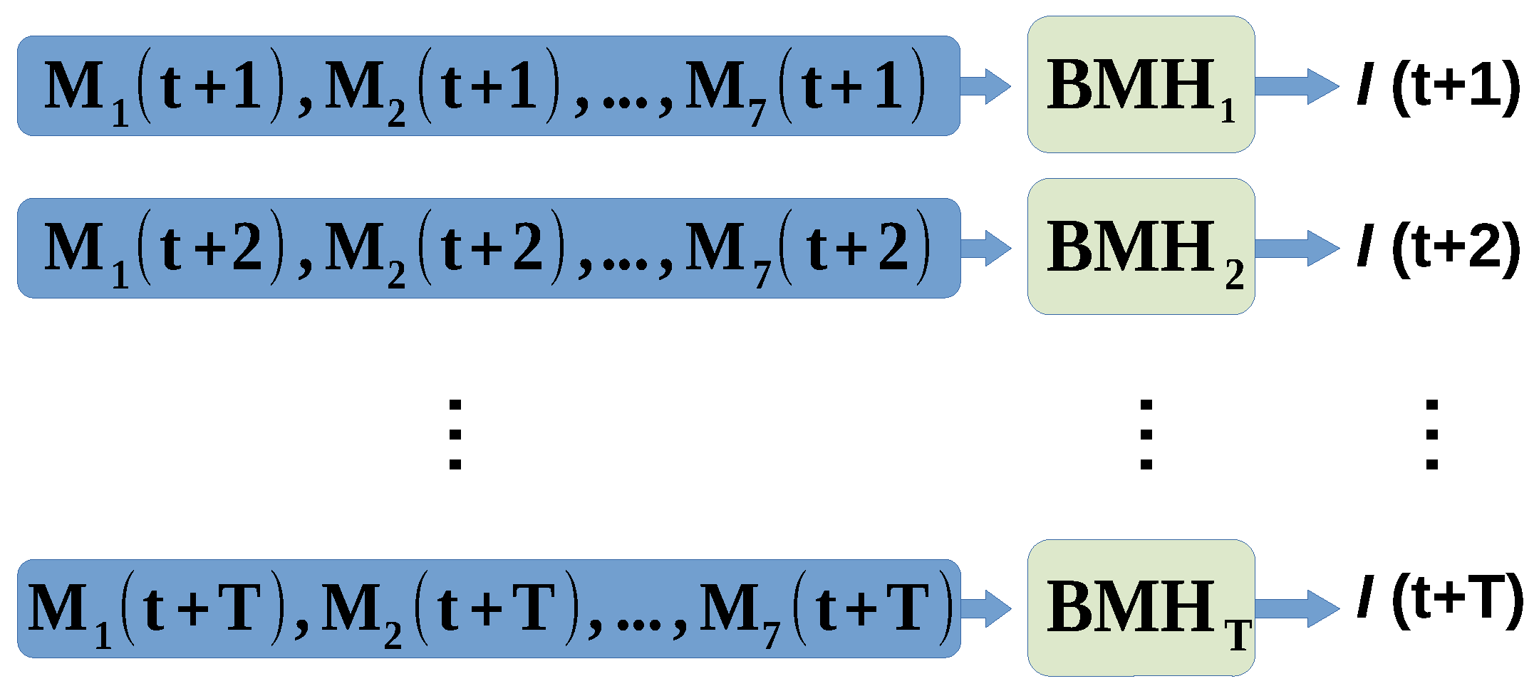
The horizon approach consists of constructing as many ML blending models as forecasting horizons, one for each horizon (T in our study case). Figure A1 shows the scheme of the horizon approach, with BMH h being the blending model for horizon h, with h = 1,…, T (with T = 90). As can be seen in Figure A1, the inputs to the BMH h models are the irradiance predictions of the M i models at horizon h ( M 1 (t + h), M 2 (t + h), …, M 7 (t + h)), and the output is the blending irradiance forecast at that horizon (I(t + h)). This approach involves training T ML blending models specialized on the data for each time horizon.
Figure A1. Horizon blending approach: one model BMH h per forecast horizon h, with h = 1, 2, …, T. Each BMH h is trained with irradiance predictions of the M i models at time t + h, M i (t + h).
Remotesensing 15 02328 g0a1
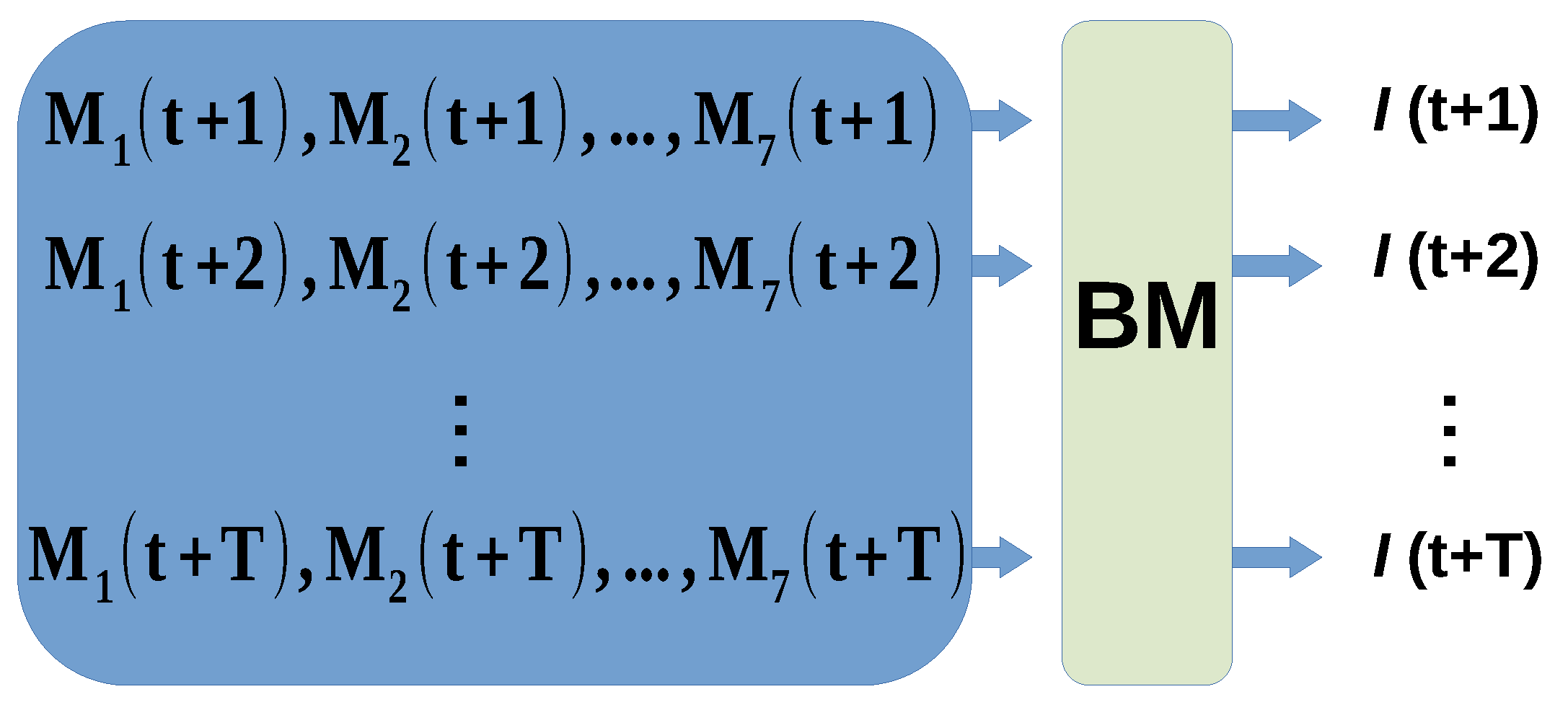
Another way of addressing the blending of the seven models M i is the general approach, which consists of constructing a single ML model that combines the predictions of the M i models for all forecasting horizons. Figure A2 shows the scheme of this approach. In this case, the ML blending model, BM, receives as input the predictions of the seven models for all horizons, from h = 1 to h = T, that is, M 1 (t + 1), M 2 (t + 1), …, M 7 (t + 1)); M 1 (t + 2), M 2 (t + 2), …, M 7 (t + 2)); …; M 1 (t + T), M 2 (t + T), …, M 7 (t + T)). Thus, the BM model will be trained with all the data and without depending on the forecasting horizon. Once the BM model was trained, it was used to predict the irradiance for each horizon, I(t + 1), I(t + 2), …, I(t + T), using only the inputs corresponding to each horizon. That is, to predict I(t + 1), the irradiance predictions of the M i models at t + 1 were used, to predict I(t + 2), the predictions of the M i models at t + 2 were used, and so on for all prediction horizons involved in this study.
Figure A2. General blending approach: a single model BM was trained with data belonging to all horizons, h = 1, …, T. In order to predict irradiance for a particular horizon h, I(t + h), the predictions of the M i models at that horizon, M i (t + h), were used as inputs to BM.
Remotesensing 15 02328 g0a2

Appendix B. Linear and RF algorithms

The linear approximation consisted of a linear combination of the p model inputs x j , as shown in Equation (A1). In this case, these inputs would depend on the type of model (horizon or general), as is described in Section 3.1. Given a dataset ( x 1 , y 1 ), …, ( x M , y M ), the coefficients c j were fit so as to minimize the summation of squared residuals between the response variable y and the linear model predictions y ^ . For this article, linear models were fit by ordinary least squares optimization using the scikit-learn library [61]:
y ^ ( x ) = y ^ ( x 1 , x 2 , , x p ) = c 0 + j = 1 p c j x j
The non-linear ML method used in this work was RF [69]. RF is a machine learning technique based on ensembles, which can be used for classification, or regression, as in this case. Ensembles are models made of several base models h 1 , h 2 , …, h N . In particular, RF for regression is an ensemble whose base models h j are regression trees (Figure A3). Each tree h j makes predictions by sending x down the tree until it reaches a leaf, where a prediction is computed by averaging all the observations ( x i , y i ) that reached that leaf during the training process. Following Meinshausen and Ridgeway [70], the RF ensemble itself makes predictions by averaging the predictions of each of the trees h j in the ensemble, as is described in Equation (A2) (and graphically depicted in Figure A3):
y ^ ( x ) = 1 N j = 1 N h j ( x )
The main aim of RF is improving the regression error by reducing the variance of the model, which in turn is achieved by adding randomness to the training of each of the base models. RF uses two techniques for this purpose: bagging and feature bagging. Bagging works by training each tree h j with a bootstrapped random sample of the original dataset ( x 1 , y 1 ), …, ( x M , y M ). Feature bagging adds randomness to the training process by using a random subset of m features instead of all p available predictors. This is carried out by randomizing the standard regression tree training method. The standard way of fitting regression trees is by means of a recursive process, which starts by selecting the best of the p features for the root node, and by repeating this selection process for each of the nodes in the next level of the tree. The best feature is the one that splits the training samples into two groups in such a way that the mean squared error of the two groups is lower than the error of the set of initial samples. The process that grows the tree is deterministic, although it can be randomized by randomly selecting m features (with m < < p ) before selecting the best feature for each of the nodes in the tree (instead of selecting the best feature out of all p available features, as in the standard method). Thus, tree training becomes stochastic since a different tree will be obtained every time it is trained, even if the same training sample is used.
The performance of any ML method depends on the values of its hyper-parameters. The main hyper-parameters of RF are the number of trees in the ensemble N and the size m of the random feature subset. Moreover, hyper-parameters that control the depth of each of the trees in the ensemble are also commonly used. Trees are grown until a stopping condition is satisfied, which in this work is controlled by two hyper-parameters: (1) the minimum sample size required for further growing the tree, and (2) the maximum tree depth. In this work, RF hyper-parameters were tuned by random search. This is a process that randomly samples hyper-parameter values, trains a model with the selected hyper-parameters, and evaluates it using a subset of the training sample. This process is repeated as many times as required to obtain a good combination of hyper-parameter values (500 times in this study). In this work, hyper-parameters were obtained via random search as follows:
  • The number of trees N was sampled from a uniform distribution between 50 and 5000 trees.
  • The size of the random feature subset m was sampled out of two values, p and log 2 p , as these two values are commonly used in the literature.
  • The maximum depth was sampled from a uniform distribution between 5 and 50.
  • The minimum number of samples was in the range of 2–20.
Both RF and random search hyper-parameter tuning implementations used for this work belong to the scikit-learn library [61].
Figure A3. Random forest graphical scheme.
Remotesensing 15 02328 g0a3

References

  1. Murdock, H.E.; Gibb, D.; Andre, T.; Sawin, J.L.; Brown, A.; Ranalder, L.; Collier, U.; Dent, C.; Epp, B.; Hareesh Kumar, C.; et al. Renewables 2021-Global Status Report. 2021. Available online: https://www.ren21.net/wp-content/uploads/2019/05/GSR2021_Full_Report.pdf (accessed on 2 February 2023).
  2. Renné, D.S. Emerging meteorological requirements to support high penetrations of variable renewable energy sources: Solar energy. In Weather Matters for Energy; Springer: Berlin/Heidelberg, Germany, 2014; pp. 257–273. [Google Scholar]
  3. Haupt, S.E. Short-range forecasting for energy. In Weather & Climate Services for the Energy Industry; Palgrave Macmillan: Cham, Switzerland, 2018; pp. 97–107. [Google Scholar]
  4. Yang, D.; Wang, W.; Gueymard, C.A.; Hong, T.; Kleissl, J.; Huang, J.; Perez, M.J.; Perez, R.; Bright, J.M.; Xia, X.; et al. A review of solar forecasting, its dependence on atmospheric sciences and implications for grid integration: Towards carbon neutrality. Renew. Sustain. Energy Rev. 2022, 161, 112348. [Google Scholar] [CrossRef]
  5. Diagne, M.; David, M.; Lauret, P.; Boland, J.; Schmutz, N. Review of solar irradiance forecasting methods and a proposition for small-scale insular grids. Renew. Sustain. Energy Rev. 2013, 27, 65–76. [Google Scholar] [CrossRef]
  6. Inman, R.H.; Pedro, H.T.; Coimbra, C.F. Solar forecasting methods for renewable energy integration. Prog. Energy Combust. Sci. 2013, 39, 535–576. [Google Scholar] [CrossRef]
  7. Yang, D.; Kleissl, J.; Gueymard, C.A.; Pedro, H.T.; Coimbra, C.F. History and trends in solar irradiance and PV power forecasting: A preliminary assessment and review using text mining. Sol. Energy 2018, 168, 60–101. [Google Scholar] [CrossRef]
  8. Samu, R.; Calais, M.; Shafiullah, G.; Moghbel, M.; Shoeb, M.A.; Nouri, B.; Blum, N. Applications for solar irradiance nowcasting in the control of microgrids: A review. Renew. Sustain. Energy Rev. 2021, 147, 111187. [Google Scholar] [CrossRef]
  9. Zhang, C.; Wu, J.; Zhou, Y.; Cheng, M.; Long, C. Peer-to-Peer energy trading in a Microgrid. Appl. Energy 2018, 220, 1–12. [Google Scholar] [CrossRef]
  10. Agoua, X.G.; Girard, R.; Kariniotakis, G. Short-term spatio-temporal forecasting of photovoltaic power production. IEEE Trans. Sustain. Energy 2017, 9, 538–546. [Google Scholar] [CrossRef]
  11. Heng, J.; Wang, J.; Xiao, L.; Lu, H. Research and application of a combined model based on frequent pattern growth algorithm and multi-objective optimization for solar radiation forecasting. Appl. Energy 2017, 208, 845–866. [Google Scholar] [CrossRef]
  12. Urquhart, B.; Ghonima, M.; Nguyen, D.A.; Kurtz, B.; Chow, C.W.; Kleissl, J. Chapter 9—Sky-Imaging Systems for Short-Term Forecasting. In Solar Energy Forecasting and Resource Assessment; Kleissl, J., Ed.; Academic Press: Boston, MA, USA, 2013; pp. 195–232. [Google Scholar] [CrossRef]
  13. Kazantzidis, A.; Tzoumanikas, P.; Blanc, P.; Massip, P.; Wilbert, S.; Ramirez-Santigosa, L. 5-Short-term forecasting based on all-sky cameras. In Renewable Energy Forecasting; Kariniotakis, G., Ed.; Woodhead Publishing Series in Energy; Woodhead Publishing: Shaxton, UK, 2017; pp. 153–178. [Google Scholar] [CrossRef]
  14. Rodríguez-Benítez, F.J.; López-Cuesta, M.; Arbizu-Barrena, C.; Fernández-León, M.M.; Pamos-Ureña, M.Á.; Tovar-Pescador, J.; Santos-Alamillos, F.J.; Pozo-Vázquez, D. Assessment of new solar radiation nowcasting methods based on sky-camera and satellite imagery. Appl. Energy 2021, 292, 116838. [Google Scholar] [CrossRef]
  15. Peng, Z.; Yu, D.; Huang, D.; Heiser, J.; Yoo, S.; Kalb, P. 3D cloud detection and tracking system for solar forecast using multiple sky imagers. Sol. Energy 2015, 118, 496–519. [Google Scholar] [CrossRef]
  16. Schmidt, T.; Kalisch, J.; Lorenz, E.; Heinemann, D. Evaluating the spatio-temporal performance of sky-imager-based solar irradiance analysis and forecasts. Atmos. Chem. Phys 2016, 16, 3399–3412. [Google Scholar] [CrossRef]
  17. Nouri, B.; Wilbert, S.; Kuhn, P.; Hanrieder, N.; Schroedter-Homscheidt, M.; Kazantzidis, A.; Zarzalejo, L.; Blanc, P.; Kumar, S.; Goswami, N.; et al. Real-Time Uncertainty Specification of All Sky Imager Derived Irradiance Nowcasts. Remote Sens. 2019, 11, 1059. [Google Scholar] [CrossRef]
  18. Dittmann, A.; Holland, N.; Lorenz, E. A new sky imager based global irradiance forecasting model with analyses of cirrus situations. Meteorol. Z. 2021, 101–113. [Google Scholar] [CrossRef]
  19. Fernández-León, M.; Pacheco, G.; Bolinaga, B.; Campa, L.; Lara-Fanego, V.; Valenzuela, J.M. Solar thermal energy predictability for the grid (STEP4Grid). In Proceedings of the AIP Conference Proceedings, Cape Town, South Africa, 13–16 October 2016; AIP Publishing LLC: Melville, NY, USA, 2016; Volume 1734, p. 080001. [Google Scholar]
  20. Nouri, B.; Noureldin, K.; Schlichting, T.; Wilbert, S.; Hirsch, T.; Schroedter-Homscheidt, M.; Kuhn, P.; Kazantzidis, A.; Zarzalejo, L.; Blanc, P.; et al. Optimization of parabolic trough power plant operations in variable irradiance conditions using all sky imagers. Sol. Energy 2020, 198, 434–453. [Google Scholar] [CrossRef]
  21. Schmidt, T.; Calais, M.; Roy, E.; Burton, A.; Heinemann, D.; Kilper, T.; Carter, C. Short-term solar forecasting based on sky images to enable higher PV generation in remote electricity networks. Renew. Energy Environ. Sustain. 2017, 2, 23. [Google Scholar] [CrossRef]
  22. Anagnostos, D.; Schmidt, T.; Cavadias, S.; Soudris, D.; Poortmans, J.; Catthoor, F. A method for detailed, short-term energy yield forecasting of photovoltaic installations. Renew. Energy 2019, 130, 122–129. [Google Scholar] [CrossRef]
  23. Lorenz, E.; Heinemann, D. Prediction of Solar Irradiance and Photovoltaic Power. In Comprehensive Renewable Energy; Sayigh, A., Ed.; Elsevier: Oxford, UK, 2012; pp. 239–292. [Google Scholar] [CrossRef]
  24. Blanc, P.; Remund, J.; Vallance, L. Short-term solar power forecasting based on satellite images. In Renewable Energy Forecasting; Elsevier: Amsterdam, The Netherlands, 2017; pp. 179–198. [Google Scholar]
  25. Ramírez, L.; Vindel, J. Forecasting and nowcasting of DNI for concentrating solar thermal systems. In Advances in Concentrating Solar Thermal Research and Technology; Blanco, M.J., Santigosa, L.R., Eds.; Woodhead Publishing Series in Energy; Woodhead Publishing: Shaxton, UK, 2017; pp. 293–310. [Google Scholar] [CrossRef]
  26. Rodríguez-Benítez, F.J.; Arbizu-Barrena, C.; Huertas-Tato, J.; Aler-Mur, R.; Galván-León, I.; Pozo-Vázquez, D. A short-term solar radiation forecasting system for the Iberian Peninsula. Part 1: Models description and performance assessment. Sol. Energy 2020, 195, 396–412. [Google Scholar] [CrossRef]
  27. Holmlund, K.; Grandell, J.; Schmetz, J.; Stuhlmann, R.; Bojkov, B.; Munro, R.; Lekouara, M.; Coppens, D.; Viticchie, B.; August, T.; et al. Meteosat Third Generation (MTG): Continuation and innovation of observations from geostationary orbit. Bull. Am. Meteorol. Soc. 2021, 102, 1–71. [Google Scholar] [CrossRef]
  28. Prasad, A.A.; Kay, M. Prediction of Solar Power Using Near-Real Time Satellite Data. Energies 2021, 14, 5865. [Google Scholar] [CrossRef]
  29. Antonanzas, J.; Urraca, R.; de Pison, F.M.; Antonanzas, F. Optimal solar tracking strategy to increase irradiance in the plane of array under cloudy conditions: A study across Europe. Sol. Energy 2018, 163, 122–130. [Google Scholar] [CrossRef]
  30. Dersch, J.; Schroedter-Homscheidt, M.; Gairaa, K.; Hanrieder, N.; Landelius, T.; Lindskog, M.; Mueller, S.C.; Santigosa, L.R.; Sirch, T.; Wilbert, S. Impact of DNI nowcasting on annual revenues of CSP plants for a time of delivery based feed in tariff. Meteorol. Z. 2019, 28, 235–253. [Google Scholar] [CrossRef]
  31. Alonso-Montesinos, J.; Polo, J.; Ballestrín, J.; Batlles, F.; Portillo, C. Impact of DNI forecasting on CSP tower plant power production. Renew. Energy 2019, 138, 368–377. [Google Scholar] [CrossRef]
  32. Litjens, G.; Worrell, E.; van Sark, W. Assessment of forecasting methods on performance of photovoltaic-battery systems. Appl. Energy 2018, 221, 358–373. [Google Scholar] [CrossRef]
  33. Haupt, S.E.; Casado, M.G.; Davidson, M.; Dobschinski, J.; Du, P.; Lange, M.; Miller, T.; Mohrlen, C.; Motley, A.; Pestana, R.; et al. The use of probabilistic forecasts: Applying them in theory and practice. IEEE Power Energy Mag. 2019, 17, 46–57. [Google Scholar] [CrossRef]
  34. Voyant, C.; Notton, G.; Kalogirou, S.; Nivet, M.L.; Paoli, C.; Motte, F.; Fouilloy, A. Machine learning methods for solar radiation forecasting: A review. Renew. Energy 2017, 105, 569–582. [Google Scholar] [CrossRef]
  35. Ahmed, R.; Sreeram, V.; Mishra, Y.; Arif, M. A review and evaluation of the state-of-the-art in PV solar power forecasting: Techniques and optimization. Renew. Sustain. Energy Rev. 2020, 124, 109792. [Google Scholar] [CrossRef]
  36. Yagli, G.M.; Yang, D.; Srinivasan, D. Automatic hourly solar forecasting using machine learning models. Renew. Sustain. Energy Rev. 2019, 105, 487–498. [Google Scholar] [CrossRef]
  37. Vislocky, R.L.; Fritsch, J.M. Improved model output and statistics through model consensus. Bull. Am. Meteorol. Soc. 1995, 76, 1157–1164. [Google Scholar] [CrossRef]
  38. Lorenz, E.; Kühnert, J.; Heinemann, D. Short term forecasting of solar irradiance by combining satellite data and numerical weather predictions. In Proceedings of the 27th European PV Solar Energy Conference (EU PVSEC), Frankfurt, Germany, 24–28 September 2012; Volume 2428, p. 44014405. [Google Scholar]
  39. Haupt, S.E.; Kosović, B.; Jensen, T.; Lazo, J.K.; Lee, J.A.; Jiménez, P.A.; Cowie, J.; Wiener, G.; McCandless, T.C.; Rogers, M.; et al. Building the Sun4Cast System: Improvements in Solar Power Forecasting. Bull. Am. Meteorol. Soc. 2018, 99, 121–136. [Google Scholar] [CrossRef]
  40. Nouri, B.; Blum, N.; Wilbert, S.; Zarzalejo, L.F. A Hybrid Solar Irradiance Nowcasting Approach: Combining All Sky Imager Systems and Persistence Irradiance Models for Increased Accuracy. Solar RRL 2022, 6, 2100442. [Google Scholar] [CrossRef]
  41. Boukabara, S.A.; Krasnopolsky, V.; Penny, S.G.; Stewart, J.Q.; McGovern, A.; Hall, D.; Hoeve, J.E.T.; Hickey, J.; Huang, H.L.A.; Williams, J.K.; et al. Outlook for Exploiting Artificial Intelligence in the Earth and Environmental Sciences. Bull. Am. Meteorol. Soc. 2021, 102, E1016–E1032. [Google Scholar] [CrossRef]
  42. Zhou, Y.; Liu, Y.; Wang, D.; Liu, X.; Wang, Y. A review on global solar radiation prediction with machine learning models in a comprehensive perspective. Energy Convers. Manag. 2021, 235, 113960. [Google Scholar] [CrossRef]
  43. Pedro, H.T.; Coimbra, C.F.; David, M.; Lauret, P. Assessment of machine learning techniques for deterministic and probabilistic intra-hour solar forecasts. Renew. Energy 2018, 123, 191–203. [Google Scholar] [CrossRef]
  44. Sun, Y.; Venugopal, V.; Brandt, A.R. Short-term solar power forecast with deep learning: Exploring optimal input and output configuration. Sol. Energy 2019, 188, 730–741. [Google Scholar] [CrossRef]
  45. Fouilloy, A.; Voyant, C.; Notton, G.; Motte, F.; Paoli, C.; Nivet, M.L.; Guillot, E.; Duchaud, J.L. Solar irradiation prediction with machine learning: Forecasting models selection method depending on weather variability. Energy 2018, 165, 620–629. [Google Scholar] [CrossRef]
  46. Dewangan, C.L.; Singh, S.; Chakrabarti, S. Combining forecasts of day-ahead solar power. Energy 2020, 202, 117743. [Google Scholar] [CrossRef]
  47. Wolff, B.; Kühnert, J.; Lorenz, E.; Kramer, O.; Heinemann, D. Comparing support vector regression for PV power forecasting to a physical modeling approach using measurement, numerical weather prediction, and cloud motion data. Sol. Energy 2016, 135, 197–208. [Google Scholar] [CrossRef]
  48. Aguiar, L.M.; Pereira, B.; Lauret, P.; Díaz, F.; David, M. Combining solar irradiance measurements, satellite-derived data and a numerical weather prediction model to improve intra-day solar forecasting. Renew. Energy 2016, 97, 599–610. [Google Scholar] [CrossRef]
  49. Qing, X.; Niu, Y. Hourly day-ahead solar irradiance prediction using weather forecasts by LSTM. Energy 2018, 148, 461–468. [Google Scholar] [CrossRef]
  50. Huertas-Tato, J.; Aler, R.; Galván, I.M.; Rodríguez-Benítez, F.J.; Arbizu-Barrena, C.; Pozo-Vázquez, D. A short-term solar radiation forecasting system for the Iberian Peninsula. Part 2: Model blending approaches based on machine learning. Sol. Energy 2020, 195, 685–696. [Google Scholar] [CrossRef]
  51. Long, C.N.; Dutton, E.G. BSRN Global Network Recommended QC Tests, V2. x. 2010. Available online: https://epic.awi.de/id/eprint/30083/1/BSRN_recommended_QC_tests_V2.pdf (accessed on 2 February 2023).
  52. Li, Q.; Lu, W.; Yang, J. A Hybrid Thresholding Algorithm for Cloud Detection on Ground-Based Color Images. J. Atmos. Ocean. Technol. 2011, 28, 1286–1296. [Google Scholar] [CrossRef]
  53. Weinzaepfel, P.; Revaud, J.; Harchaoui, Z.; Schmid, C. DeepFlow: Large displacement optical flow with deep matching. In Proceedings of the ICCV-IEEE International Conference on Computer Vision, Sydney, Australia, 1–8 December 2013; pp. 1385–1392. [Google Scholar] [CrossRef]
  54. Rigollier, C.; Bauer, O.; Wald, L. On the clear sky model of the ESRA—European Solar Radiation Atlas—with respect to the Heliosat method. Sol. Energy 2000, 68, 33–48. [Google Scholar] [CrossRef]
  55. Schmetz, J.; Pili, P.; Tjemkes, S.; Just, D.; Kerkmann, J.; Rota, S.; Ratier, A. An introduction to Meteosat second generation (MSG). Bull. Am. Meteorol. Soc. 2002, 83, 977–992. [Google Scholar] [CrossRef]
  56. Rigollier, C.; Lefèvre, M.; Wald, L. The method Heliosat-2 for deriving shortwave solar radiation from satellite images. Sol. Energy 2004, 77, 159–169. [Google Scholar] [CrossRef]
  57. Liberzon, A.; Gurka, R.; Taylor, Z. Openpiv Home Page. 2009. Available online: https://openpiv.sourceforge.net/ (accessed on 2 February 2023).
  58. Nonnenmacher, L.; Coimbra, C.F. Streamline-based method for intra-day solar forecasting through remote sensing. Sol. Energy 2014, 108, 447–459. [Google Scholar] [CrossRef]
  59. Zhang, C.; Ma, Y. Ensemble Machine Learning: Methods and Applications; Springer: Berlin/Heidelberg, Germany, 2012. [Google Scholar]
  60. Louppe, G.; Wehenkel, L.; Sutera, A.; Geurts, P. Understanding variable importances in forests of randomized trees. Adv. Neural Inf. Process. Syst. 2013, 26, 431–439. [Google Scholar]
  61. Pedregosa, F.; Varoquaux, G.; Gramfort, A.; Michel, V.; Thirion, B.; Grisel, O.; Blondel, M.; Prettenhofer, P.; Weiss, R.; Dubourg, V.; et al. Scikit-learn: Machine learning in Python. J. Mach. Learn. Res. 2011, 12, 2825–2830. [Google Scholar]
  62. Hammer, A.; Kühnert, J.; Weinreich, K.; Lorenz, E. Short-term forecasting of surface solar irradiance based on Meteosat-SEVIRI data using a nighttime cloud index. Remote Sens. 2015, 7, 9070–9090. [Google Scholar] [CrossRef]
  63. Romano, F.; Cimini, D.; Cersosimo, A.; Di Paola, F.; Gallucci, D.; Gentile, S.; Geraldi, E.; Larosa, S.; Nilo, S.T.; Ricciardelli, E.; et al. Improvement in surface solar irradiance estimation using HRV/MSG data. Remote Sens. 2018, 10, 1288. [Google Scholar] [CrossRef]
  64. Aksakal, S.K. Geometric accuracy investigations of SEVIRI high resolution visible (HRV) level 1.5 Imagery. Remote Sens. 2013, 5, 2475–2491. [Google Scholar] [CrossRef]
  65. Debaecker, V.; Kocaman, S.; Saunier, S.; Garcia, K.; Bas, S.; Just, D. On the geometric accuracy and stability of MSG SEVIRI images. Atmos. Environ. 2021, 262, 118645. [Google Scholar] [CrossRef]
  66. Miller, S.D.; Rogers, M.A.; Haynes, J.M.; Sengupta, M.; Heidinger, A.K. Short-term solar irradiance forecasting via satellite/model coupling. Sol. Energy 2018, 168, 102–117. [Google Scholar] [CrossRef]
  67. Sirch, T.; Bugliaro, L.; Zinner, T.; Möhrlein, M.; Vazquez-Navarro, M. Cloud and DNI nowcasting with MSG/SEVIRI for the optimized operation of concentrating solar power plants. Atmos. Meas. Tech. 2017, 10, 409–429. [Google Scholar] [CrossRef]
  68. López-Cuesta, M.; Jiménez-Garrote, A.; Aler-Mur, R.; Galván-León, I.; Tovar-Pescador, J.; Pozo-Vazquez, D. Improving ASI-Based Solar Radiation Nowcasting by Using Automatic Cloud Type Recognition Methods (No. EMS2022-166). Technical Report. In Proceedings of the Copernicus Meetings, Bonn, Germany, 4–9 September 2022. [Google Scholar]
  69. Breiman, L. Random forests. Mach. Learn. 2001, 45, 5–32. [Google Scholar] [CrossRef]
  70. Meinshausen, N.; Ridgeway, G. Quantile regression forests. J. Mach. Learn. Res. 2006, 7, 983–999. [Google Scholar]
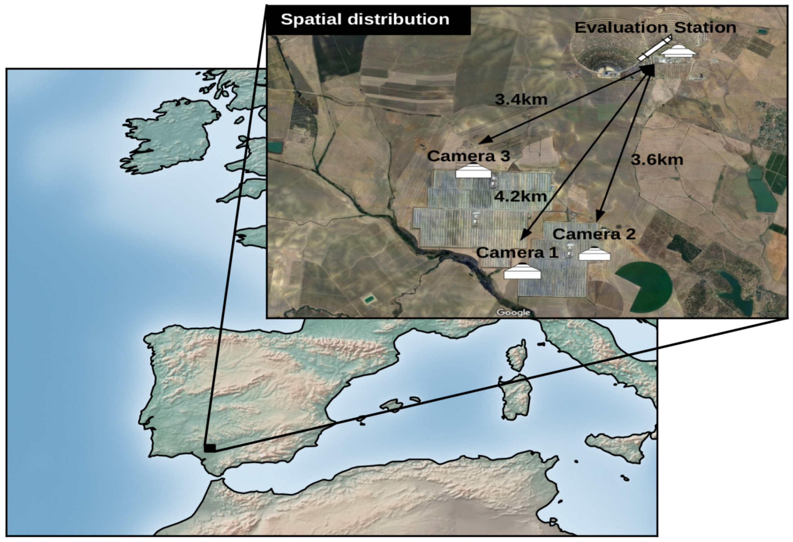
Figure 1. Location of the Abengoa Solúcar platform, and spatial distribution of the three cameras, ceilometer and radiation ground data station.
Remotesensing 15 02328 g001
Figure 2. Forecasting samples available as a function of the forecasting horizon. The black line represents the total number of samples, the yellow line represents the training dataset samples (2/3) and the red line represents the validation dataset samples (1/3).
Remotesensing 15 02328 g002
Figure 3. Flow chart of the procedure used to evaluate the blending approaches and the blending models.
Remotesensing 15 02328 g003
Figure 4. Feature importance (%) of the different model inputs for the General-RF Sats and Sats & ASI experiments. The values are displayed for GHI (left) and DNI (right).
Remotesensing 15 02328 g004
Figure 5. rRMSE values (%), as a function of the forecasting horizon, for the nine experiments conducted using the general approach and the RF model. Ninety-minute-ahead one-minute time resolution forecasts are displayed at the left for GHI and at the right for DNI.
Remotesensing 15 02328 g005
Figure 6. As in Figure 5 but for the forecasting skill (FS).
Remotesensing 15 02328 g006
Figure 7. rRMSE values (%), as a function of the forecasting horizon, for the best-performing experiments for GHI (Sats & ASI) and DNI (Sats) and the two reference models (average and optimal).
Remotesensing 15 02328 g007
Figure 8. As in Figure 7, although for the forecasting skill.
Remotesensing 15 02328 g008
Table 1. Nowcasting models included in the study, along with their main characteristics.
Model Input AcronymModel Main Characteristics
ASI-1, ASI-2 and ASI-3Single ASI-based, forecasts spatial resolution ∼meters
ASI-meanMean of the ASI-1, ASI-2 and ASI-3 models forecasts
Sat-LRLow Resolution satellite-images-based forecasts, 5 km spatial resolution
Sat-HRHigh resolution satellite-images-based forecasts, 1 km spatial resolution
Smart-PersistenceSmart persistence (data-driven) model, no error at lead time 0
Table 2. Sets of input models involved in the different experiments evaluated in this work. The acronyms of the set are listed in the left column and the model inputs involved are listed in the right column.
Name of Input Models SetModels Input Involved
Sat-LRSat-LR, Smart-Persistence
Sat-HRSat-HR, Smart-Persistence
ASIASI-1, Smart-Persistence
Sat-LR & ASISat-HR, ASI-1, Smart-Persistence
Sat-HR & ASISat-HR, ASI-1, Smart-Persistence
SatsSat-LR, Sat-HR, Smart-Persistence
Sats & ASIASI-1, Sat-LR, Sat-HR, Smart-Persistence
Sats & ASIsASI-1, ASI-2, ASI-3, Sat-LR, Sat-HR, Smart-Persistence
Sats & ASI-meanASI-mean, Sat-LR, Sat-HR, Smart-Persistence
Table 3. Evaluation results of a set of experiments using the general and horizon blending approaches and both the linear and RF blending models. The rRMSE(%) values of the experiments are displayed for both the GHI and DNI forecast. Error values are computed considering all the forecasts samples, from 1 to 90 min-ahead forecasts. Bold text indicates the best-performing experiments for GHI and DNI forecast.
Models Input Set
 Blending
Model
Blending
Approach
Sat-LRSat-HRASISat-LR
& ASI
Sat-HR
& ASI
SatsSats
& ASI
Sats
& ASIs
Sats
& ASI-mean
GHIRFGeneral30.731.035.127.128.122.921.822.821.9
Horizon33.734.737.933.034.032.532.932.432.5
LinearGeneral32.933.035.832.632.831.931.831.731.7
Horizon32.833.636.933.034.232.733.033.332.9
DNIRFGeneral58.856.565.057.260.042.243.243.643.5
Horizon63.567.070.264.767.262.264.364.163.0
LinearGeneral62.363.367.362.262.761.261.060.860.5
Horizon61.563.970.863.465.961.062.662.461.3
Disclaimer/Publisher’s Note: The statements, opinions and data contained in all publications are solely those of the individual author(s) and contributor(s) and not of MDPI and/or the editor(s). MDPI and/or the editor(s) disclaim responsibility for any injury to people or property resulting from any ideas, methods, instructions or products referred to in the content.