Abstract
The ocean front has a non-negligible role in global ocean–atmosphere interactions, marine fishery production, and the marine military. Hence, obtaining the positions of the ocean front is crucial in oceanic research. At present, the positioning method of recognizing an ocean front has achieved a breakthrough in the mean dice similarity coefficient (mDSC) of above 90%, but it is difficult to use to achieve rapid extraction in emergency scenarios, including marine fisheries and search and rescue. To reduce the its dependence on machines and apply it to more requirements, according to the characteristics of an ocean front, a multi-scale model SQNet (Simple and Quick Net) dedicated to ocean front position recognition is designed, and its perception domain is expanded while obtaining current scale data. In experiments along the coast of China and the waters of the Gulf of Mexico, it was not difficult to find that SQNet exceedingly reduced running time while ensuring high-precision results (mDSC of higher than 90%). Then, after conducting intra-model self-comparison, it was determined that expanding the perceptual domain and changing the weight ratio of the loss function could improve the accuracy and operational efficiency of the model, which could be better applied in ocean front recognition.
1. Introduction
An ocean front is a narrow excess zone between two or more water masses with significantly different characteristics, and the characteristic quantities of one or more hydrographic elements determine the location of the front area [1]. An ocean front area usually has a strong oblique pressure structure, and various material exchange activities are very active and occupy an important position in the sea–air interaction [2]. The vicinity of fronts is often accompanied by seawater irradiation [3,4], which collects marine oil, heavy metals and other substances and is of non-negligible significance to marine environmental protection; the sea area is usually rich in nutrients, which provide food and a living environment for sea creatures and fish, and have certain value in the development of marine fisheries. In addition, the ocean front also affects the structure of the flow field in the ocean. By identifying the junction line of different water masses through the ocean front, we can study the spatial and temporal changes of the water masses and the characteristics of the generation and elimination potential [5]. Therefore, understanding the spatial distribution and temporal variation of ocean fronts is of great significance in marine environmental protection, marine fishery construction, fishing planning, and the generation and change of marine habitats [6], and is of great significance to the understanding of mesoscale ocean phenomena and the structure of ocean flow fields. It is also of great value to the marine military and so on.
There are two main traditional methods with which to extract the position of an ocean front. One is based on a gradient algorithm used to set the threshold for processing, including the gradient algorithm [7,8,9,10] and canny algorithm [11]; the other is also a mathematical physical method of reformulating the algorithm, using wavelet analysis [12,13], an algorithm based on the law of gravity [14,15,16,17], the histogram method [18,19,20,21,22], the mathematical morphology method [23,24,25,26], and the entropy theory algorithm [27,28,29]. In addition to the above methods, domestic and foreign scholars have optimized the traditional methods for ocean front detection. Simhadri et al. [30] proposed a method based on wavelet analysis to extract marine feature information. Additionally, based on wavelet analysis, Xue et al. [13] performed feature extraction on the ocean front of the Gulf Stream. Hopkins et al. introduced weighted local likelihood, and [31] proposed a method based on statistical models. However, traditional methods rely on artificial threshold settings and are susceptible to noise interference, making it challenging to accomplish high-precision marine front position identification using them.
The model based on deep learning has been applied in recent years, and researchers have used neural network-based ocean front detection methods for ocean front detection. Before 2019, Lima et al. [32] first attempted to detect the location of ocean front occurrence (in a binary classification) using convolutional neural networks and achieved high-recognition accuracy at a patch-level resolution. To improve Lima’s method, Sun et al. [33] performed an overlapping sampling of ocean front areas and obtained a fine-grained location of the ocean front. However, their algorithm only detected the location of the ocean front at the patch level. As image recognition rapidly matured after 2019, many scholars applied deep-learning-based image recognition in ocean front recognition. Li et al. considered ocean front detection as an edge detection problem and successively proposed a bidirectional edge detection network (BEDNet) [34] and weak edge identification network (WEIN) [35], which can identify the location of an. ocean front at the pixel level. Li et al. [36] used UNet to detect and locate ocean front areas in grayscale SST (sea surface temperature) images with accurate results. Xie et al. [37] used LSENet to detect and locate multiple ocean fronts in color SST gradient maps, achieving an ocean front recognition breakthrough with a mDSC higher than 90%. Up until now, multiple artificial intelligence methods have completely exceed traditional methods in terms of recognition accuracy. Currently, LSENet is the method with the highest ocean front recognition accuracy in public.
Although LSENet performs best among the existing methods with its high accuracy, it is difficult to accomplish intense time-sensitive marine work such as typhoon search and rescue, fishing production, and red tide monitoring with it. For this situation, this paper proposes a new simple and efficient model (SQNet) to meet the demand for high-precision and high-efficiency ocean front identification, the innovations of which are as follows. Firstly, its single-pixel ocean front-sensing domain is augmented from that of traditional methods and other deep learning methods. Secondly, a three-layer network is built to enable a fusion analysis of multi-scale recognition results. Thirdly, its loss function is adapted for the small sample of the ocean front to rapidly improve its recognition accuracy for ocean front classes.
2. Dataset
Currently, there is no available dataset that is expert-validated, so we created two ocean front datasets: the China coastal dataset and the Gulf of Mexico dataset. First, we collected daily SST data from the National Oceanic and Atmospheric Administration (NOAA)’s advanced very-high-resolution radiometer (AVHRR) with a spatial resolution of 0.05°. Then, we selected data within these two study seas and generated SST gradient maps.
The following equation calculated the SST gradient maps for the Sobel gradient operator.
where and denote the horizontal and vertical gradient of the current coordinate point, respectively, A denotes the matrix of 3 × 3 neighborhoods of the current coordinate point, * denotes the convolution operation, and G denotes the coordinate point of the gradient value of the current coordinate point. In addition, the “jet” color map of the Python library Matplotlib is used for the color mapping of SST gradient values to generate SST gradient maps. To prevent overfitting and to increase the amount of data, we used random photometric distortion, random image cropping, and random image flipping to enhance the data in both datasets.
For the Chinese offshore dataset, this paper selected the Chinese offshore region (117.975–130.975°E, 23.025–40.025°N) and the period 2015–2018 (1461 samples in total) to generate a gradient map that is 340 × 260 in size as shown in Figure 1.
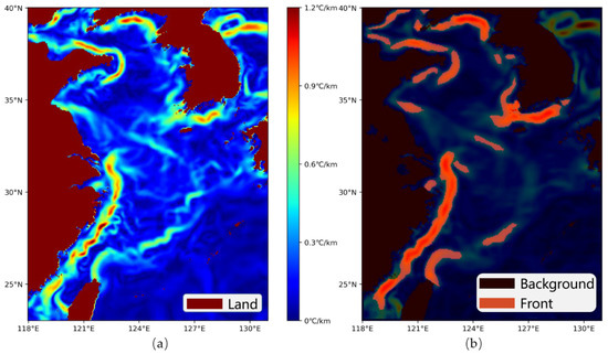
Figure 1.
Labeled data in Chinese offshore dataset. (a) Original SST gradient map. (b) Labeled result.
At present, previous research results are combined to obtain the distribution of the main fronts in the Chinese offshore; in the Bohai Sea, there are Bohai coastal fronts and Bohai Strait fronts [38]. In the Yellow Sea, there are more ocean fronts, including the Shandong Peninsula fronts, the Korean Peninsula west coast fronts (including West Korea Bay fronts and Ganghwa Bay fronts), Jeju Island west coast fronts, and Jeju Island east coast fronts [39,40]. The hydrographic condition is rather complex in the East China Sea. Additionally, there is an abundance of ocean fronts, mainly Jiangsu coastal fronts, Yangtze estuarine circulation fronts, Kuroshio fronts, and Zhejiang and Fujian coastal fronts in the East China Sea [41,42]. In the northern South China Sea, there are the Taiwan shallow fronts, Guangdong coastal fronts, Pearl River mouth nearshore fronts, Hainan Island eastern coastal fronts, Beibu Gulf front, and Kuroshio intrusion fronts [43]. Based on the multivariate satellite fusion data, Shi et al. [44] used the gradient detection algorithm to study the offshore waters of China, and the SST information was obtained as shown in Table 1.

Table 1.
Months of existence of the offshore sea temperature front of China [44].
Based on the abovementioned expert experience and existing research, we used method [44,45] to divide each pixel in the image into two categories: one is the ocean front class, and a certain point is the front class, which is the geographical location corresponding to the pixel at the corresponding time of the ocean front; the other type is the background class, and a certain point is the background class, where no ocean front appears.
To evaluate the performance of the model, data from the whole year of 2018 (365 samples in total) were selected as the test set. To ensure that the test set contained the ocean front for all seasons, the remaining data (1096 samples in total) from 2015 to 2017 were used as the training set for model training. To facilitate data enhancement and model downsampling, we reshaped the size of the original input images to 352 × 352 × 3 using the zero padding method.
For the Gulf of Mexico dataset, the Gulf of Mexico’s current front region is selected in this paper as (80.0–98.2°W, 17.8–31.0°N), and the period 2007–2011 is selected (1824 samples in total), to generate gradient maps that are 264 × 364 in size, as shown in Figure 2.

Figure 2.
Labeled data in the Gulf of Mexico dataset. (a) Original SST gradient map. (b) Labeled result.
Within the study area, the fronts are highly influenced by wind forcing, wind-driven Ekman transport and related upwelling/downwelling, river discharge, ocean currents, and topography. They may be associated with local tides due to their geographical location [46]. Within the Gulf of Mexico region, ocean fronts are mainly found in the coastal and current areas.
Based on the abovementioned expert experience and existing research, we the use method in [1,44] to divide each pixel in the image into two categories: one is the ocean front class, and a certain point is the front class, which is the geographical location corresponding to the pixel at the corresponding time of the ocean front; the other type is the background class, and a certain point is the background class, where no ocean front appears.
To evaluate the performance of the model, data from 2010 to 2011 (729 samples in total) were selected as the test set. To ensure that the test set contained the ocean front for all seasons of the year, the remaining data from 2007 to 2009 (1095 samples in total) were used as the training set for model training. Finally, a zero padding method was used to reshape the size of the original input images to 384 × 384 × 3 to facilitate data enhancement.
3. Model Description
To achieve high operational efficiency and attain an mDSC higher than 90%, the LSENet model was used as the control model in this paper. The following is an introduction to LSENet and SQNet.
3.1. LSENet
Figure 3 shows the overview of LSENet model. It consists of two parts:
- (1)
- An encoder–decoder part (E1–E5 and D1–D4), which is responsible for feature extraction and feature processing;
- (2)
- A head part, which is responsible for outputting detection results.

Figure 3.
Overview of the LSENet [37].
Figure 4 shows the structure of an encoder with two branches. The branch at the bottom is composed of two convolution blocks to extract and analyze the features of the image. In this branch, the feature map is fed into two convolution blocks to generate a new feature map . Here, H and W represent the height and width of the feature map, respectively, while C0 and C represent the number of channels. The upper branch is the CSU proposed in this article. The design idea of CSU is to let the model comprehensively analyze the input feature map at the channel level, judge the classes of fronts contained in the feature map, and introduce the seasonality of ocean fronts into the model by seasonal feature encoding. In this branch, feature map first goes through a global average pooling layer and the dimension is compressed to . Then, a fully connected layer (ReLU activation function) is used to reduce the number of channels to C/2 for seasonal feature insertion. After concatenating the monthly one-hot encoded seasonal features, the number of channels is changed to 12 + C/2, and then, a fully connected layer (ReLU activation function) is used to generate the feature map . After summing each pixel of the feature map B2 and B1, the output feature map of the encoder is obtained by downsampling. The structures of the decoder and the encoder differ only in the last sampling layer, where D2–D4 uses upsampling layer, and D1 does not use the sampling layer [37].

Figure 4.
Structure of an encoder in LSENet [37].
The head part consists of detection branch and attention branch (as shown in Figure 5). The detection branch at the bottom contains only a convolutional layer of 1 × 1 convolution kernel to map the number of channels to the desired number of classes N (N = 12), and then, the model detection result is obtained by Softmax function. For the upper LA branch, a given feature map is first fed into an averaged pooling layer to obtain the feature map , where r is the downsampling coefficient. Here, r is set to 8 and 24 in the Chinese offshore dataset and the Gulf of Mexico dataset, respectively, based on multiple experiments. Then, the feature map C1 is fed into a convolution block for feature learning, and the size of the feature map is reshaped to , where Cl represents the number of channels. Each pixel in this feature map can be considered as a high abstraction of the feature of the region with the size of r × r. At the same time, location encoding is added into the attention branch to enhance the model’s sensitivity to geographical location. Next, the location encoded feature map is input into several convolution blocks for feature learning, and then, the result is converted into values between 0 and 1 through a convolution block with Sigmoid activation function. These values represent the attention weights of the model for different channels of each region. The resulting attention weight map is upsampled by bilinear interpolation and is elementwise multiplied by the results of the detection branch. Finally, an elementwise summation operation is performed with the result of multiplication and the result of detection branch to further optimize the detection result [37].
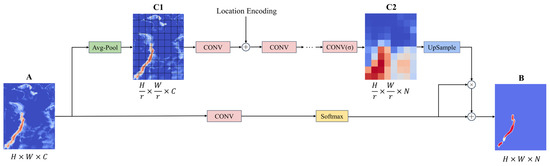
Figure 5.
Structure of the head part in LSENet [37].
3.2. SQNet
Figure 6 shows the overview of our model. The model contains two main parts, the multi-scale analysis of the original dataset in blocks 1–3 on the left and the fusion output of the results of a multi-scale analysis of blocks 1–3 on the right. The fusion output of the original resolutions L0, 2L0, and 4L0 is realized in the model, and the perceptual domain expansion of the ocean front is realized in blocks 1–3.

Figure 6.
Structure of the SQNet.
Figure 7 shows the structure of blocks 1–3 in the SQNet. Within blocks 1–3, the input image information is processed by convolutional operations, and each block consists of a transfer branch and an analysis branch. In the case of Block 2, its input is RH/2 × W/2 × C. In the branch, the input information is gradually extracted by 3 × 3, 4 × 4 and 5 × 5 perceptual information of the ocean front, then passed to the 2 × 2 pool for downsampling and then passed to Block 3; in the analysis branch, after 3 × 3, 4 × 4 and 5 × 5 convolution operations, a 1 × 1 convolution is performed and then summed up. The information of ocean front at the current 2L0 resolution is extracted for the output.

Figure 7.
Structure of blocks 1–3in SQNet.
After the operation of blocks 1–3, the analysis results at L0, 2L0, and 4L0 resolutions are obtained, and 2L0 and 4L0 are upsampled to obtain the analysis results at the L0 and 2L0 resolutions. At the L0 resolution, convolutional fusion from the merging of the L0 and 2L0 resolutions results occurs; at 2L0 resolution, convolutional fusion from the merging of the 2L0 and 4L0 resolutions results occurs; at 4L0 resolution, convolutional fusion from the 4L0 resolution occurs. Finally, the results at the three resolutions are summed up and convolved, and the Softmax classifier classifies the ocean front as the output results of SQNet.
Since the ocean front belongs to data of a small sample, the proportion of the ocean front in a single image is about 5–20%. The traditional binary-classification cross-entropy loss is used to calculate the loss value, and a low loss value indicates low initial recognition accuracy. Thus, calculating cross-entropy loss has poor performance in reflecting ocean front recognition accuracy. For this reason, the model assigns weights to binary-classification cross-entropy loss objects when calculating the loss value. We change the weight function to realize the correlation between high-recognition accuracy and a low loss value so that the optimal solution weight can easily be set during training. The formula is as follows:
3.3. Differences and Similarities
Both LSENet and SQNet enable the multi-scale analysis of raw data through data downsampling. However, to improve recognition accuracy, LSENet performs seasonal result analysis and introduces the attention result mechanism; the introduction of the two methods makes the model run more computationally intensively and increases the running time to a certain extent. SQNet achieves accuracy improvement by changing the convolution kernel size to improve the perceptual domain, fusing the analysis results under multiple resolutions and changing the loss function to adapt to ocean front recognition. Among them, changing the size of the convolution kernel to improve the perceptual domain and fusing the analysis results under multiple resolutions using the method of augmenting the convolution kernel and summing up after convolution increases the total computation of the model to a lesser extent, while changing the loss function can enable the model to quickly find the weight data with higher accuracy during the training process and reduce the running time to improve the model’s efficiency under the same epoch of training. After the experiments, it can be seen that it takes about 0.4 h to run 20 epochs of training in the original perceptual domain, 1 h to run 20 epochs by boosting the perceptual domain and changing the loss function, and 2.5 h for LSENet, and SQNet can find the best weights more quickly for engineering activities such as monitoring when the accuracy is similar. A summary of the similarities and differences between LSENet and SQNet is shown in Table 2.
Table 2.
Difference and Similarity between LSENet and SQNet.
4. Experimental Environment and Results
4.1. Parameter Setting and Evaluation Metrics
Based on the constructed dataset, all experiments in this paper were executed on an NVIDIA GeForce GTX1050Ti graphic processing unit (GPU; GPU is used to speed up model training and does not improve model accuracy) with one 8 GB RAM and implemented using the open-source deep learning libraries Keras and TensorFlow to simulate the acquisition of ocean front locations in emergencies. To compare with other semantic segmentation models, we set the same parameters for our model and the comparison model as follows: batch size is set to 4 or the highest batch the computer can run, and LSENet uses traditional binary cross-entropy as the loss function, Adam [47] as the optimizer, and 1 × 10⁻³ as the initial learning rate when the loss of the validation set does not decrease. The learning rate is reduced to half of the previous learning rate for three consecutive periods using a learning rate decay strategy.
In this paper, we use the mean intersection-to-merge ratio (mIoU) and the mean dice similarity coefficient (mDSC) as evaluation metrics, as mIoU and mDSC are commonly used evaluation metrics in the field of semantic segmentation. The essence of the intersection of union (IoU) is to calculate the ratio of intersection and union of ground truth and predicted segmented datasets. This ratio can be expressed as the sum of true positives (TP) divided by false positives (FP), false negatives (FN), and TP, as shown in the following equation:
𝐼𝑜𝑈 = 𝑇𝑃/(𝐹𝑃+𝐹𝑁+𝑇𝑃)
DSC is usually used to measure the similarity of two sample sets and can be expressed as the following equation:
mIoU and mDSC are the averages of IoU and DSC, respectively. Their complete equations are as follows:
where denotes the number of pixels belonging to class i when it is detected as class j (= TP when i and j are equal, and = FN when i and j are not equal). Similarly, denotes the FP case when i and j are not equal. k denotes the total number of classes.
4.2. LSENet vs. SQNet Comparison Results
To accurately measure whether or not SQNet can guarantee high accuracy as well as ocean front position recognition efficiently, LSENet was selected as the control model for the experiment. In Table 3, it is not difficult to find that within the same epoch, SQNet has a more significant advantage than LSENet does in terms of accuracy, mIoU, mDSC, and running time for ocean front recognition; for another 40 epoch run, the accuracy improvement of the model LSENet is weaker than that of SQNet. To achieve the goal of high accuracy (an mDSC higher than 90%), SQNet is completed by within 2 h in the existing environment and LSENet is not satisfied within 15 h.
Table 3.
Model comparison results of Chinese coastal dataset.
The epoch80 results of SQNet and epoch120 results of LSENet were weighted to be validated by test data. As shown in Figure 8, the ocean front near Kuroshio in spring was obvious, and the identification results of the two methods were similar. The summer ocean front was mainly concentrated in the northern coast, and the identification of SQNet was with high accomplishment. In autumn, the coastal front was mainly extracted and more fragments could be detected. In the results, SQNet identification shows high continuity and identification capacity (with more pixels identified) in the coastal areas of Zhejiang and Fujian provinces and the coast of Liaodong Peninsula. In winter, two methods recognized coastal fronts and Kuroshio fronts.

Figure 8.
Comparison results along the Chinese coast ((a–d) the spring image, (e–h) the summer image, (i–l) the autumn image, and (m–p) the winter image; (a,e,i,m) the input image, (b,f,j,n) the true value, (c,g,k,o) LSENet result, (d,h,l,p) and SQNet result).
The experimental environment is set to the same as that in the Chinese coastal dataset. The results are shown in the Table 4; within the same epoch, SQNet has a more distinct advantage than LSENet in ecognition accuracy, mIoU, mDSC, and running time for marine fronts. To achieve high accuracy (mDSC higher than 90%), SQNet takes 2 h under the existing environment, and LSENet does not achieve it within 15 h.
Table 4.
Model comparison display for the Gulf of Mexico dataset.
The epoch80 results of SQNet and epoch120 results of LSENet were weighted to be validated by the test data. As shown in Figure 9, the ocean front near the Gulf Stream in spring is obvious, and the identification results of the two methods are similar. In summer, ocean fronts are mainly concentrated in the southern coast, and the identification of SQNet is relatively complete. In autumn, the northern coastal front is mainly extracted. SQNet performs with high-recognition continuity, and the identification is complete. In winter, coastal fronts are identified similarly. However, for fronts near the Gulf Stream, SQNet performed better than LSENet did at identification.

Figure 9.
Comparison results for the Gulf of Mexico ((a–d) the spring image, (e–h) the summer image, (i–l) the autumn image, and (m–p) the winter image; (a) the input image, (b) the true value, (c) the LSENet result, and (d) the SQNet result).
4.3. Comparison Results of Parameter Adjustment within the SQNet Model
After the above two sets of experiments, it is obvious that SQNet perfornms high-quality ocean front recognition tasks in a shorter time by increasing the ocean front perception domain and changing the loss function in contrast to the high computational power required for LSENet. After, we further increased the perceptual domain of ocean front and transformed the loss function to verify whether or not SQNet can effectively improve recognition accuracy. The experiments in this section used the Chinese coastal dataset.
To increase the perceptual domain of the ocean front, SQNet changes from the traditional three 3 × 3 convolutions to three 3 × 3, 4 × 4, and 5 × 5 convolutions to extract ocean front information. In the experiments, the three 3 × 3, 4 × 4, and 5 × 5 convolution kernels in SQNet were changed to three 3 × 3 convolution kernels for the control experiments. From Table 5, it is evident that SQNet achieves greater improvement in ocean front class accuracy, mIoU, and mDSC than the control model does after the same number of epochs of training. As a result, the accuracy of SQNet after 20 epochs of training is higher than that of the control model after 40 epochs of training.
Table 5.
Convolution kernel change comparison results.
To verify the improvement in accuracy of SQNet in only changing the loss function, the initial weights are set. The ratio of ocean front class to background class weights is set as 1:1, 2:1, 3:1, 4:1, 1:2, 1:3, and 1:4. For the experiments, where 1:1 is the weight ratio in the traditional dichotomous cross-entropy and 3:1 is the weight ratio in the SQNet model, the weights with background class accuracy of 29.37%, ocean front class accuracy of 6.08%, mIoU of 17.73%, and mDSC of 28.44% are used as the initial weights. The statistics of the results after 20 epochs of training are as follows: the 3:1 used in SQNet could highly improve the rate of recognition of the ocean front with the same number of epochs. As shown in Table 6 and Figure 10, compared to the weight ratio in traditional-binary cross-entropy, there is a 0.5% improvement in the ocean front. The background class weight is unified to 1, and when the weight of ocean front is increased to 3, the recognition accuracy of its ocean front improves with the increase in the weight of ocean front. Moreover, when the weight of ocean fronts is increased from 3 to 4, the accuracy of recognition of the ocean front decreases. As seen in Figure 10, it is considered in this paper that there is a maximum value between the range of ratio 2:1 and 4:1. On the left of this value, accuracy increases as weights increase; on the right of the value, accuracy decreases as weights increase because the position of that value varies with ratios of ocean front class and background class in the dataset. Therefore, for most datasets, this paper suggests setting a weight ratio to one that is close to 3:1.
Table 6.
Comparison results of weight ratio parameters.

Figure 10.
Relationship between recognition accuracy and weighting ratio for marine fronts.
5. Discussion
At present, the methods that can accomplish high precision identification of ocean fronts (mDSC>90%) are LSENet and SQNet, which can be seen in Table 7. In this paper, As shown in Table 8, under the same running environment with the same dataset, SQNet has more advantages compared to LSENet. However, from the objective analysis, the running environment in LSENet’s paper is highly enhanced compared with this paper, and the running environment in this paper cannot be restored to LSENet due to the limitation of various external environments. it is difficult to predict the comparison between the two under the high memory and strong GPU environment. All experiments in LSENet are performed on an NVIDIA RTX 3080 graphic processing unit (GPU) with 10 10-GB memory. All experiments in SQNet are performed on an NVIDIA GeForce GTX1050Ti graphic processing unit (GPU) with 8GB memory.
Table 7.
Comparision with exsiting ocean front detection method.
Table 8.
Model comparison results.
The innovation points of this article are as follows: 1. In the model design, the perception domain of the ocean front is expanded, although the running time is increased, but compared with LSENet, the complexity of SQNet operation is not high, and with other optimizations, it can meet the needs of efficient and high-quality identification. This optimization direction is proposed based on the own characteristics of ocean fronts, combining them with convolution kernels in machine learning. 2. According to the characteristics of the ocean front dataset, the loss function is adjusted, which not only improves the operation efficiency, but also improves the model results to a certain extent. The ocean front dataset is a small sample dataset in most cases, and the ocean front class accounts for a low proportion of the total. In the training after the model design, it is especially important to use the loss function that can truly reflect the change of its marine front class identification accuracy. 3. Compared with LSENet citing high-computation functions, SQNet relies on the characteristics of ocean front to design a lightweight model that is easy to apply to real-world urgent tasks. In order to better apply to the real world, it is an inevitable choice to suppress the increase in computational volume and computational difficulty while improving the accuracy. Looking for data characteristics from the data itself can g better shorten the running time than using high computation algorithms to fuse machine learning models.
Upon internal discussion, we observed the following shortcomings.
Since there is no publicly available expert-labeled ocean front dataset, this paper uses a self-built dataset labeled according to previous experience and papers for dataset generation, which inevitably caused some reduction in accuracy. If conditions permit it and funding support is available, we will attempt to produce and calibrate publicly available ocean front datasets. In the case of global data labeling or data labeling of research hotspots, we will first label the daily SST gradient maps for one year, and then check and revise them after disorganization to ensure that the accuracy of the dataset is above 90%.
Based on the constructed dataset, all experiments in this paper were executed on an NVIDIA GeForce GTX1050Ti graphic processing unit (GPU) with one 8 GB RAM and implemented using the open-source deep learning libraries Keras and TensorFlow to simulate the acquisition of ocean front locations in emergencies. The LSENet [37] configuration environment is much stronger than in this article, so the operating time of LSENet is very different from the operating environment mentioned in the paper. If there is more financial support, high-configuration computers may be used for re-experimentation or algorithmic innovation.
To achieve the goal of fast and accurate identification of ocean fronts, this paper does not use algorithmic fusion in the neural network structure, but instead makes changes to the details of the neural network structure to avoid high computing processes that reduce efficiency. There are three points to note about the proposed changes to the details of the network structure.
Firstly, three resolution analysis results can be integrated and output. The resolution of the input data should be 0.05°. If the data resolution is too low after an exceeding number of downsampling operations, it is difficult to extract effective information from it, which means it may produce interference information, resulting in the final fusion output with a lower mDSC. With no downsampling operation, the information of larger scale ocean fronts can be coarsely captured, resulting in the final front class accuracy being lower. Thus, mDSC cannot meet the requirements.
Secondly, the perceptual domain of ocean fronts can be expanded. The 3 × 3 convolution kernel used in the conventional method is similar to that used in the traditional method, which is prone to non-recognition or over-recognition for large fronts such as plume fronts. The improved 3 × 3, 4 × 4, and 5 × 5 convolution kernels are used to extract the input information. After the experiment, we found that the data accuracy could be improved under the same epoch. If the conditions allow it, the comparison of larger convolution kernels can be carried out afterward. For example, we can conduct an experiment to verify whether or not the 7 × 7 convolution kernel pair can achieve substantial accuracy improvement compared with the 3 × 3 application. Furthermore, more experiments could be conducted to compare the accuracy improvement with the joint use of 3 × 3, 7 × 7 and 10 × 10.
Thirdly, the weight ratio in the loss function can be changed. Due to the small percentage of ocean front classes in the ocean front dataset (about 5–20%), the traditional loss function has poor performance in achieving a fast search for optimal solution weights. In the experiment, we found that mDSC increases with the weight ratio from 1:4 to 2:1, and mDSC is similar from 2:1 to 4:1, with the best result at 3:1. The weight ratio in this experiment corresponds to that of the Chinese coastal self-labeled dataset used. If other datasets are used, experiments should be conducted first to find the extreme value point in the curve of the weight ratio and data accuracy fitting function. Then, the weight ratio of this point should be used for ocean front identification extraction.
The extraction of ocean front positions conducted in this paper was directed at sea surface temperature (SST). The datasets for extraction can be chlorophyll concentration, salinity, and suspended sediment concentration (in Class II water bodies), in subsequent work. In addition, the time information, geographic information, and marine background environment information could be merged to be set as the input image. Additionally, the image with information on the time, latitude, and longitude and the current information could be merged, and the ocean front information could be output, which could be applied in the study of sea–air exchange, fisheries, and sound speed research.
6. Conclusions
Realizing the combination of image recognition and target detection using deep learning techniques, this paper obtains ocean front pixel-level recognition results based on a multi-scale fast recognition SQNet model.
First, we build two datasets, the China coastal dataset and the Gulf of Mexico dataset, and label the images in two categories (ocean front and background).
The second step, to establish a model, based on the research of the predecessors and our own exploration, we mainly change the model in two ways: the first is y carryin out multi-scale fusion to find ocean front information at different scales. The second is by expanding the perception domain of the ocean front, changing the original three 3 × 3 convolution kernels to 3 × 3, 4 × 4 and 5 × 5.
In the final model training stage, it was found that the traditional loss function in machine learning was not applicable to the ocean front dataset, and the weight ratio in the loss function was modified according to the characteristics of the ocean front.
In the experimental comparison in the same environment, we found that the change of the convolution kernel in the optimization of the model’s structure could improve the accuracy of model recognition. At the same time, the change in loss function could indeed improve the model effect and improve the accuracy of recognizing an ocean front. Combined with a variety of optimizations, SQNet can exceed LSENet in terms of both runtime and result accuracy.
Author Contributions
Conceptualization, R.N.; methodology, R.N.; validation, Q.Z.; formal analysis, Y.T.; investigation, R.N.; resources, F.G.; data curation, F.Y.; writing—original draft preparation, R.N. and Y.T.; writing—review and editing, R.N. and Y.T.; project administration, H.H.; funding acquisition, Z.H. All authors have read and agreed to the published version of the manuscript.
Funding
This research was funded by the National Key Research and Development Program of China (grant 2021YFC3101602), and National Natural Science Foundation of China (grant 61991454).
Data Availability Statement
The original sst date is from daily SST data from the National Oceanic and Atmospheric Administration (NOAA)’s advanced very-high-resolution radiometer (AVHRR) with a spatial resolution of 0.05° which can download in https://oceanwatch.pifsc.noaa.gov/erddap/griddap/goes-poes-1d-ghrsst-RAN.html.
Acknowledgments
We thank NOAA AVHRR for providing global sea surface temperature data during the study period and the staff of the Hangzhou satellite ground station, satellite data processing and sharing center, and marine satellite data online analysis platform of the State Key Laboratory of Satellite Ocean Environment Dynamics, Second Institute of Oceanography, Ministry of Natural Resources (SOED/SIO/MNR), for their help with data collection and processing.
Conflicts of Interest
The authors declare no conflict of interest.
References
- Belkin, I.M.; Cornillon, P.C.; Sherman, K. Fronts in Large Marine Ecosystems. Prog. Oceanogr. 2009, 81, 223–236. [Google Scholar] [CrossRef]
- Liu, J.; Zhang, Y. Characteristics of the spatial and temporal variation of the front at west sea of Indonesia. Mar. Forecast. 2015, 32, 14–23. [Google Scholar]
- Bost, C.-A.; Cotté, C.; Bailleul, F.; Cherel, Y.; Charrassin, J.-B.; Guinet, C.; Ainley, D.G.; Weimerskirch, H. The importance of oceanographic fronts to marine birds and mammals of the southern oceans. J. Mar. Syst. 2009, 78, 363–376. [Google Scholar] [CrossRef]
- Guo, T.; Gao, W. Phenomenon of ocean front and it impact on the sound propagation. Mar. Forecast. 2015, 32, 80–88. [Google Scholar]
- Qiu, C.; Cui, Y.; Hu, S.; Huo, D. Seasonal variation of Guangdong coastal thermal front based on merged satellite data. J. Trop. Oceanogr. 2017, 36, 16–23. [Google Scholar]
- Cui, X.; Zhou, W.; Wang, D.; Zhang, S. Fronts extraction and vectorization from raster image of sea surface temperature. J. Image Graph. 2012, 17, 1384–1390. [Google Scholar]
- Oram, J.J.; McWilliams, J.C.; Stolzenbach, K.D. Gradient-based edge detection and feature classification of sea-surface images of the Southern California Bight. Remote Sens. Environ. 2008, 112, 2397–2415. [Google Scholar] [CrossRef]
- Belkin, I.M.; O’Reilly, J.E. An algorithm for oceanic front detection in chlorophyll and SST satellite imagery. J. Mar. Syst. 2009, 78, 319–326. [Google Scholar] [CrossRef]
- Wang, F.; Liu, C. An N-shape thermal front in the western South Yellow Sea in winter. Chin. J. Oceanol. Limnol. 2009, 27, 898–906. [Google Scholar] [CrossRef]
- Liu, C.; Wang, F.. Distributions and intra-seasonal evolutions of the sea surface thermal fronts in the Yellow Sea warm current origin area. Mar. Sci. 2009, 33, 87–93. [Google Scholar]
- Wall, C.C.; Muller-Karger, F.E.; Roffer, M.A.; Hu, C.; Yao, W.; Luther, M.E. Satellite remote sensing of surface oceanic fronts in coastal waters off west–central Florida. Remote Sens. Environ. 2008, 112, 2963–2976. [Google Scholar] [CrossRef]
- Park, J.H.; Il-Seok, O. Wavelet-Based Feature Extraction from Character Images. In Proceedings of the International Conference on Intelligent Data Engineering and Automated Learning, Hong Kong, China, 21–23 March 2003. [Google Scholar]
- Xue, C.; Su, F.; Zhou, J. Extraction of Ocean Fronts Based on Wavelet Analysis. Mar. Sci. Bull. 2007, 26, 20–27. [Google Scholar]
- Sun, G.; Liu, Q.; Liu, Q.; Ji, C.; Li, X. A novel approach for edge detection based on the theory of universal gravity. Pattern Recognit. 2007, 40, 2766–2775. [Google Scholar] [CrossRef]
- Lopez-Molina, C.; Bustince, H.; Fernandez, J.; Couto, P.; De Baets, B. A gravitational approach to edge detection based on triangular norms. Pattern Recognit. 2010, 43, 3730–3741. [Google Scholar] [CrossRef]
- Zhang, C.; Chen, X. Gravitational approach to edge detection based on nonlinear filtering. J. Comput. Appl. 2011, 31, 4. [Google Scholar] [CrossRef]
- Ping, B.; Su, F.; Du, Y.; Meng, Y.; Su, W. Application of the Model of Universal Gravity to Oceanic Front Detection Near the Kuroshio Front. J. Geo-Inf. Sci. 2013, 15, 187–192. [Google Scholar] [CrossRef]
- Cayula, J.-F.; Cornillon, P. Edge Detection Algorithm for SST Images. J. Atmos. Ocean. Technol. 1992, 9, 67–80. [Google Scholar] [CrossRef]
- Ullman, D.; Brown, J.; Cornillon, P.; Mavor, T. Surface Temperature Fronts in the Great Lakes. J. Great Lakes Res. 1998, 24, 753–775. [Google Scholar] [CrossRef]
- Diehl, S.F.; Budd, J.W.; Ullman, D.; Cayula, J.-F. Geographic Window Sizes Applied to Remote Sensing Sea Surface Temperature Front Detection. J. Atmos. Ocean. Technol. 2002, 19, 1105–1113. [Google Scholar] [CrossRef]
- Belkin, I.M.; Cornillon, P. SST fronts of the Pacific coastal and marginal seas. Pac. Oceanogr. 2003, 1, 90–113. [Google Scholar]
- Yao, J.; Belkin, I.; Chen, J.; Wang, D. Thermal fronts of the southern South China Sea from satellite and in situ data. Int. J. Remote Sens. 2012, 33, 7458–7468. [Google Scholar] [CrossRef]
- Lea, S.M.; Lybanon, M. Finding mesoscale ocean structures with mathematical morphology. Remote Sens. Environ. 1993, 44, 25–33. [Google Scholar] [CrossRef]
- Xue, C.; Su, F.; Zhou, J.; Guo, Y.; Zhang, T. Extracting feature of ocean front based on mathematical morphology. Mar. Sci. 2008, 32, 57–61. [Google Scholar]
- Pi, Q.; Hu, J. Analysis of sea surface temperature fronts in the Taiwan Strait and its adjacent area using an advanced edge detection method. Sci. China Earth Sci. 2010, 53, 1008–1016. [Google Scholar] [CrossRef]
- Xiao, D. Improvements to the Detection of Ocean Fronts by Grayscale Gradient Method. China Comput. Commun. 2016, 4, 97–99+107. [Google Scholar] [CrossRef]
- Shimada, T.; Sakaida, F.; Kawamura, H.; Okumura, T. Application of an edge detection method to satellite images for distinguishing sea surface temperature fronts near the Japanese coast. Remote Sens. Environ. 2005, 98, 21–34. [Google Scholar] [CrossRef]
- Vázquez, D.P.; Atae-Allah, C.; Escamilla, P.L.L. Entropic Approach to Edge Detection for SST Images. J. Atmos. Ocean. Technol. 1999, 16, 970–979. [Google Scholar] [CrossRef]
- Sun, G.; GUo, M.; Wang, X.; Li, S. Application of Edge Detection to the Sea Surface Temperture Fronts of China East Coast. Remote Sens. Inf. 2012, 27, 61–66. [Google Scholar]
- Simhadri, K.K.; Iyengar, S.S. Wavelet-based feature extraction from oceanographic images. IEEE Trans. Geosci. Remote Sens. 1998, 36, 767–778. [Google Scholar] [CrossRef]
- Hopkins, J.; Challenor, P.; Shaw, A.G. A New Statistical Modeling Approach to Ocean Front Detection from SST Satellite Images. J. Atmos. Ocean. Technol. 2010, 27, 173–191. [Google Scholar] [CrossRef]
- Lima, E.; Sun, X.; Dong, J.; Wang, H.; Yang, Y.; Liu, L. Learning and Transferring Convolutional Neural Network Knowledge to Ocean Front Recognition. IEEE Geosci. Remote Sens. Lett. 2017, 14, 354–358. [Google Scholar] [CrossRef]
- Sun, X.; Wang, C.; Dong, J.; Lima, E.; Yang, Y. A Multiscale Deep Framework for Ocean Fronts Detection and Fine-Grained Location. IEEE Geosci. Remote Sens. Lett. 2019, 16, 178–182. [Google Scholar] [CrossRef]
- Li, Q.; Fan, Z.; Zhong, G. BEDNet: Bi-directional Edge Detection Network for Ocean Front Detection. In Neural Information Processing; Springer: Cham, Switzerland, 2020; pp. 312–319. [Google Scholar]
- Li, Q.; Zhong, G.; Xie, C.; Hedjam, R. Weak Edge Identification Network for Ocean Front Detection. IEEE Geosci. Remote Sens. Lett. 2022, 19, 1–5. [Google Scholar] [CrossRef]
- Li, Y.; Liang, J.; Da, H.; Chang, L.; Li, H. A Deep Learning Method for Ocean Front Extraction in Remote Sensing Imagery. IEEE Geosci. Remote Sens. Lett. 2022, 19, 1–5. [Google Scholar] [CrossRef]
- Xie, C.; Guo, H.; Dong, J. LSENet: Location and Seasonality Enhanced Network for Multiclass Ocean Front Detection. IEEE Trans. Geosci. Remote Sens. 2022, 60, 1–9. [Google Scholar] [CrossRef]
- Zhao, B.; Cao, D.; Li, H.; Wang, Q. Tidal mixing characters and tidal fronts phenomenons in the Bohai Sea. Acta Oceanol. Sin. 2001, 113–119. [Google Scholar] [CrossRef]
- Zheng, Y.; Ding, L.; Tan, D. Distribution Characeristics of Marine Fronts in the Southern Huanghai Sea And the Donghai Sea. J. Oceanogr. Huanghai Bohai Seas 1985, 5, 9–17. [Google Scholar]
- Xu, S.; Chen, B.; Tao, R.; Zhang, C.; Liu, H. The Temporal and Spatial Distribution Characteristics of Thermal Front in the China Seas. J. Telem.,Track. Command. 2015, 36, 62–69+74. [Google Scholar]
- Lin, C. Oceanographic Characteristics of the Kuroshio Front in the East China Sea and the Relationship with Fisheries. Donghai Mar. Sci. 1986, 4, 8–16. [Google Scholar]
- Chen, B.; Ma, L.; Zhang, C.; Li, B.; Liu, H. Ocean front analysis in subdivided sea areas by using satellite remote sea surface temperature data. Ocean. Eng. 2018, 36, 108–118. [Google Scholar]
- Chen, C. Some explanation of sea surface temperature distribution in northern South China Sea in winter. Acta Oceanol. Sin. 1983, 5, 391–395+397–398. [Google Scholar]
- Shi, Y.; Zhang, G.; Zhang, C.; Yi, X.; Liu, H.; Li, B. Research on ocean front detection in China coastal waters based on multi-source merging data. J. Telem. Track. Command. 2022, 43, 104–110. [Google Scholar]
- Hickox, R.; Belkin, I.; Cornillon, P.; Shan, Z.J.G.R.L. Climatology and seasonal variability of ocean fronts in the East China, Yellow and Bohai Seas from satellite SST data. Geophys. Res. Lett. 2000, 27, 2945–2948. [Google Scholar] [CrossRef]
- Zhang, Y.; Hu, C. Ocean Temperature and Color Frontal Zones in the Gulf of Mexico: Where, When, and Why. J. Geophys. Res. Ocean. 2021, 126, 391–395+397–398. [Google Scholar] [CrossRef]
- Kingma, D.; Ba, J. Adam: A Method for Stochastic Optimization. Comput. Sci. 2014. [Google Scholar] [CrossRef]
Disclaimer/Publisher’s Note: The statements, opinions and data contained in all publications are solely those of the individual author(s) and contributor(s) and not of MDPI and/or the editor(s). MDPI and/or the editor(s) disclaim responsibility for any injury to people or property resulting from any ideas, methods, instructions or products referred to in the content. |
© 2023 by the authors. Licensee MDPI, Basel, Switzerland. This article is an open access article distributed under the terms and conditions of the Creative Commons Attribution (CC BY) license (https://creativecommons.org/licenses/by/4.0/).