Article

Impacts of Water and Stress Transfers from Ground Surface on the Shallow Earthquake of 11 November 2019 at Le Teil (France)

1
Bureau de Recherches Géologiques et Minières, 45100 Orleans, France
2
School of Geology, Aristotle University of Thessaloniki, 54124 Thessaloniki, Greece
3
NexGen Analytics, 84330 Le Barroux, France
*
Author to whom correspondence should be addressed.
Remote Sens. 2023, 15(9), 2270; https://doi.org/10.3390/rs15092270
Submission received: 15 March 2023 / Revised: 10 April 2023 / Accepted: 19 April 2023 / Published: 25 April 2023

Abstract

:
The 4.9 Mw earthquake of 11 November 2019 at Le Teil (France) occurred at a very shallow depth (about 1 km), inducing the surface rupture of La Rouvière fault. The question was raised shortly after about the potential impact of a nearby surface quarry. Thanks to satellite differential interferometry, here, we revealed the existence of a secondary surface rupture of the quasi-parallel Bayne Rocherenard fault. A newly processed seismic cross-section allowed us to shape the three-dimensional geometry of the local three-fault system. Assuming that the earthquake was triggered by the impact of meteoric water recharge, our numerical simulations show that the hydraulic pressure gradient at depth was at a maximum during the period of 2010–2019, just before the seismic event. The estimated overpressure at the intersection of the two faults, which is the most probable place of the hypocenter, was close to 1 MPa. This hydraulic effect is about two and a half times larger than the cumulative effect of mechanical stress release due to the mass removal from the surface quarry over the two past centuries. This work suggests a rapid hydraulic triggering mechanism on a network of faults at a shallow depth after a heavy rainfall episode.

Graphical Abstract

1. Introduction

Large earthquakes usually occur along preexisting faults and plate interfaces. However, intraplate earthquakes are difficult to assess, as many damaging earthquakes are not associated with the known major faults, which are considered to have the highest seismic potential in the area [1]. Since the recurrence time of intraplate events is long, our knowledge and understanding of the fault dynamics (structure, rheology, stress loading, and interaction) are still limited, and causes other than the long-term tectonic stress loading are, therefore, considered for some earthquakes. For example, the 2008 7.9 Mw Wenchuan (China) earthquake had a total fault length of more than 200 km in the Longmenshan fault zone. Before the occurrence of the earthquake, the highest seismic potential of the area had never been attributed to the ruptured faults (causal faults) from the seismic hazard assessment [2] view point. Although the tectonic stress loading is undoubtable over the whole area, the nucleation process of this mega earthquake has been discussed in relation to the nearby Zipingpu reservoir in terms of the elastic stress change and pore pressure change [3,4,5,6,7,8]. Indeed, any positive perturbation of stress on a causal fault can be suspected of triggering an earthquake [9]. The lack of in situ measurements, however, does not allow any definitive conclusion, and the impoundment of the reservoir may have activated the shallow micro-seismicity within a few kilometers below the dam [5,6], but the link to the hypocenter of the earthquake more than 10 km away is not clear.
The anthropogenic influence on earthquake triggering has been widely studied, and several authors have produced an overview of the likely cases [10,11,12,13,14,15], covering a range of magnitude between 1 and 8. At a local scale, the micro-seismicity at Gardanne, southern France, is correlated to the flooding of the underground abandoned mining gallery, with a time lag of about ten days [16]. The driving mechanism behind the triggering is not only human-driven, but it can also be related to natural variations on the Earth’s surface, namely climate variations [17,18,19]. It is reported that the seismicity in Himalaya has a seasonal trend according to the annual monsoon season, namely large amounts of precipitation in the summer [20,21]. Among the studies analyzing the rainfall effect, the seasonal pore pressure evolution was discussed through fluid diffusion in the limestone of southeastern Germany [19]. The seismicity triggered by rainfall in the karstic domain, in Switzerland, was studied through a fluid diffusion model in a poro-elastic context [22]. The hypothesis of “hydro-seismicity” developed by John K. Costain [23,24,25,26] attributes most intraplate and near-intraplate earthquakes to the dynamics of the hydrologic cycle. Such hydraulic perturbations may occur from a few to 10 km away if a permeably connected fault system exists. In France, a correlation between heavy rainfall and small earthquakes was shown in the Western Provence around the Nîmes Fault [27] and in the Provence Alps at Castellane [28].
The 2019 4.9 Mw Le Teil (France) earthquake heavily damaged nearby areas [29,30]. Regardless of its moderate magnitude, this earthquake ruptured the shallowest part of the known fault (only the first 2 km depth at most) and showed rupture traces on the ground surface (Figure 1). The area had been known for some historical earthquakes; however, earthquakes of this magnitude with surface ruptures had hardly been taken into account in local/regional seismic hazard assessments [31]. Previously, some authors pointed out that a nearby limestone quarry may have contributed to the stress loading on the causal fault [32,33,34]. The best-inferred epicenter is probably located not inside but rather southwest of the surface quarry, using the seismograms available from the mainshock and aftershocks [35]. In contrast to a purely mechanical view, here, we will investigate the hypothesis of an earthquake triggered by the water transfer from the ground surface. Indeed, the studied area suffered from heavy rainfall during the month before the seismic event. Therefore, a permeably connected fault system may play a role of conducting the pore pressure change at depth. We focus on the local hydraulic system in the study area. The movement of moisture in partially saturated media is simulated using a 3D diphasic flow, double-permeability model, with the soil moisture data recorded during the period of 2010–2019 as surface boundary and the Rhône River as edge boundary conditions. We will finally discuss the possible triggering mechanism by comparing the results of the hydraulic model with those of a mechanical model that simulates the mass withdrawal due to the quarry exploitation in a similar geological configuration. We will try to answer two key questions: (1) How large is the hydraulic overpressure due to the meteoric water recharge compared to the Coulomb stress change due to the mass withdrawal from the surface quarry? (2) Is the estimated location of the maximum hydraulic overpressure consistent with the estimated hypocenter location?

2. Materials and Methods

2.1. Differential Synthetic-Aperture Radar Interferometry (DInSAR) Using Sentinel-1 Data

Spaceborne differential SAR interferometry (DInSAR) has been widely used during the past decades to track land subsidence or uplift related to groundwater extraction or underground gas storage [37]. The same method has also been successfully used for identifying ruptures due to earthquakes and quantifying the co-seismic motion [38,39]. Sentinel-DInSAR was applied to measure the surface displacement along the sensor’s Line of Sight (LOS), which is the sensor-to-target direction. This method measures the projection of real surface motion along the LOS and provides 1D displacement measurements. These displacements are relative in space and time, as they are spatially related to a reference point, and temporally to the date of the first available satellite acquisition. In order to reduce the loss of coherence effect, four interferograms with short six-day timespans around the date of 11 November 2019 were produced using Sentinel-1 data (Table S1). The processing is based on the Gamma processing software (https://gamma-rs.com, accessed on 16 January 2021). Only one interferogram (named A059—orbit 59 in ascending mode) resulted as interpretable because of a poor coherence on the surface rupture zones for the three others. In order to interpret this interferogram for identifying and quantifying surface ruptures, an additional unwrapping step is required (Figure 2). For this step, we used the Minimum Cost Flow procedure implemented in Gamma [40].
The visual examination allowed a first estimation of the LRF rupture location and the positions of the extremities of a candidate for the BRF rupture (Figure 3). In order to obtain additional candidates, we added the positions of faults extracted from a 1:50,000 geological map [36]. These faults were imported in the tool for profile stacking and displacement estimation using the Cosi-corr software [41,42], in order to be applied to our unwrapped interferogram. Figures S1–S3 illustrate the use of the tool on different parts of LRF and BRF. Twenty lateral profiles were automatically generated by the tool, perpendicularly to the candidate on LRF/BRF, and three were manually added on BRF. Our objective was first to validate points on the fault candidate as reliable observations if significant differential motion between each side of the profile was observed, and then to quantify this motion. In addition, if the “jump” on the displacement profile is not exactly on the candidate’s position, this procedure allows to adjust the position by displacing the candidate according to the jump’s position. Finally, the obtained points were connected in order to obtain a continuous rupture trace. This proposed procedure was found to be sensitive enough for interpreting the initial interferometric information, and the obtained results were in fairly good agreement with the surface rupture evidence (Figure 3). Although it could not be fully exhaustive and minor motions could be missed, this method provided an accurate and reliable representation of the surface traces of LRF and BRF, and a quantification of their surface displacements was proposed (Figure 3).
Furthermore, some unwrapping issues can occur close to the ruptures for two main reasons. First, some sectors of the area have poor coherence because of possible surface changes that occurred during the six-day timespan due to the earthquake itself or due to the presence of locally vegetated land covers. Secondly, the observed motion on the ruptures was larger than quarter of the wavelength (i.e., 14 mm). One noteworthy point is the fact that the two parallel ruptures introduced a specific unwrapping issue (illustrated in Figure S4). This may have influenced the location and quantification of the rupture traces. Examples of unwrapping issues can be found in [43,44]. For these reasons, it is important to choose an interpretation of the interferogram consistent with the prior knowledge of faults (e.g., ground observations or boreholes). The consequence is that it introduces an ambiguity on the distribution of the measured slip between the two faults. As this ambiguity cannot be resolved only on the basis of the information of one interferogram, here, we will use additional observations (i.e., surface rupture evidence and boreholes’ cores).

2.2. Hydraulic Model Using ComPASS

ComPASS is an open platform using state-of-the-art numerical schemes to discretize multiphase Darcian flows on generic unstructured meshes [45,46]. We adopted a so-called hybrid dimensional model coupling a 3D model of the “matrix” with a 2D model in “fault planes” using ComPASS (Appendix A).

2.2.1. Hydraulic Parameters in Matrix/Fault

The hydraulic parameters in the Barremian/Urgonian limestones are highly variable in the host rock, the damaged zone, and the core fault [47,48,49,50]. The continuous medium (“matrix”) and the fault elements are characterized by a large range of porosity and permeability. In the Urgonian carbonates at Low-Noise Underground Laboratory (LSBB) of Russel, about 90 km southeast of Le Teil, the observations showed the presence of discontinuities (joints, veins, faults, and stylolites) that influence the hydraulic properties from the core to the reservoir scale. The measured porosity varied from 1% to 20% and the permeability varied in a range between 10−17 m2 and 5 × 10⁻¹² m2 close to the fault core [47]. In the “matrix”, a permeability of 10−16 m2 and a porosity of 20% (Table 1) were chosen, corresponding to typical values in the host rock measured in the group of samples with higher porosity and permeability. In the “fault”, the fault permeability varied in the range of high values between 10−12 m2 and 10−11 m2 based on in situ measurements in fault zones [48]. The hydraulic parameters are displayed in Table 1 for the base cases using the in situ soil moisture at a 30 cm depth at Berzème (SM30), and in Table A1 for the additional cases using the surface soil moisture acquired by the SMOS satellite (SSM).

2.2.2. Soil Moisture (SM30) Data at the Berzème Station

The SMOSMANIA network (Soil Moisture Observing System) is based on the Meteorological Automatic Network Integrated Application of Météo-France. The stations form a Mediterranean–Atlantic transect following the marked climatic gradient between the two coastlines. The station at Berzème of SMOSMANIA is located at less than 15 km from Le Teil quarry (Figure A1). The vegetation on these sites is made up of natural fallow land, cut once or twice a year. Since 24 April 2015, four soil moisture probes have been installed per station at depths of 5, 10, 20, and 30 cm. These capacitance probes use the dielectric permittivity properties of the soil to estimate the volumetric soil moisture content. The data at a depth of 30 cm (noted SM30) are used in the reference ComPASS simulations as boundary conditions for the whole nodes at the top surface, except for those belonging to the Rhône River. The soil moisture content is the quantity of water contained in the soil. The normalized water content (or effective saturation, Se) is calculated at the Berzème station following Equation (1):
S e = S M 30 θ r ω θ r ,
where SM30 is the volumetric water content at a 30 cm depth (raw data), θ r is the residual water content (about 12% between 2015 and 2019), and the saturated water content is equivalent to porosity, ω (about 42% at 30 cm). SMOSMANIA was developed to validate remote sensing and model soil moisture estimates. The average distance between two neighboring stations is approximately 40 km, which is consistent with the spatial resolution of remote sensing soil moisture products of the SMOS satellite.

2.2.3. Surface Soil Moisture (SSM) Products Acquired by the SMOS Satellite

The first satellite mission to focus primarily on the collection of soil moisture data was the European satellite SMOS (Soil Moisture and Ocean Salinity), launched in November 2009. Here, we use the term surface soil moisture (SSM) to refer to the volumetric soil moisture in the first few centimeters (0–5 cm) of the soil. The soil moisture data acquired by SMOS are used as alternative surface boundary conditions (Appendix A). The SMOS-CATDS (Centre Aval de Traitement des Données SMOS) provides either a 3-day product or a 10-day SSM product (that contains median, minimum, and maximum values of soil moisture). Ascending and descending overpasses of the SMOS satellite are bound to show different values of the retrieved parameters that may not always be comparable, and they are, thus, separately retrieved. The data are presented over the Equal-Area Scalable Earth (EASE grid 2) [51], with a sampling of about 25 km × 25 km, and the studied area is included in two grid cells, called L1 and L2 (Figure A1). Using the Berzème station during the year 2019, we found a bias of −12.3 vol.% and a correlation coefficient of 0.49, as already observed in southwestern France by others [52]. As the residual water content, θ r , is almost zero for all three-day SSM products, the effective saturation, Se, is calculated following Equation (2) (Figure S6):
S e = S S M ω
where ω is the porosity at 5–10 cm (about 50% in the Harmonized World Soil Database). Another SSM product, called SMOSMAP-IB, is available at INRAE BORDEAUX [53]. It fuses SMOS and NASA’s SMAP satellite. We found a much better correlation coefficient of 0.7 for SMOSMAP-IB than for SMOS-CATDS. Unbiased values of Se are then calculated following Equation (3) (Figure A2):
S e = S S M + B I A S B I A S ( ω B I A S ) = S S M ( ω B I A S )
where BIAS is the bias between SSM and SM30 during the year 2019 (−11.3 vol.%).

2.3. Mechanical Model Using 3DECTM

To model the mechanical effect of mass withdrawal on the fault system, the Distinct Element Method of 3DECTM code (Version 5.2, Itasca Consulting Group Inc., Minneapolis, MN, USA), that explicitly handles discontinuities as mechanically active joints, was adopted here [54]. The Coulomb stress change is given by Δ C F F = Δ τ μ Δ σ n , where Δ τ and Δ σ n are the shear and normal stress changes (positive in compression), and μ is the frictional coefficient. The direction of τ is taken for the maximum shear stress on the given fault geometry. The mass withdrawal generates a relaxing of normal stress on LRF as well as an increase of shear stress. The Coulomb stress change, Δ C F F , related to the mass withdrawal is estimated from the difference between the two equilibrium steps (Appendix B).

2.4. Seismological Data Analysis Using the Vibration Sensor at Clauzel House (CLAU)

A vibration sensor was installed by the quarry owner in the private house Clauzel (CLAU, red triangle in Figure 1) to monitor the vibrations due to the quarry blasts. The sensor is a three-component, short-period seismograph (sampling rate at 1024 Hz). The recorded data of the mainshock include visually unnatural jumps in velocity, and this leads to unexpected levels of acceleration. The on-site visit leads us to think that the CLAU sensor has not been correctly fixed on the house floor and probably may have been impacted by the fall of miscellaneous objects around it. Although the whole waveform may not be exploitable, the first movement at the beginning of the signals could be informative. In order to verify the polarity, we checked the blast signal of 25 September 2019, for which the source location is well-known. For the given records, we removed the linear trend, applied the Butterworth bandpass filter (order of 8) between 1 and 10 Hz, and integrated once using the software SeisGram2K Seismogram Viewer v7.0.0 × 10 (www.alomax.net, accessed on 16 January 2021) for data viewing and processing. Then, we manually exploited the particle motion of this blast for a selected time window. We obtained a back azimuth of N98°E ± 20° for the true value of N111°E (Figure S7). Thus, the particle motion approximatively indicates the event direction with a margin of error of around 16°. The sensor data were used to estimate the azimuth of the mainshock of 11 November 2019, assuming the same margin of error.

3. Results

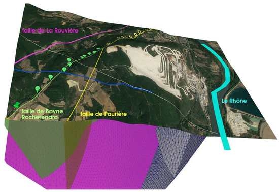
3.1. Geological Context around the Fault System

The concerned area is located in the Rhône Valley in southeastern France near Montélimar City (Figure 1). The Urgonian limestones, which were extracted from the nearby quarry, were deposited in the early cretaceous epoch, during the Upper Barremian–Lower Aptian age, and afterwards, some calcareous marlstones were deposited during the Aptian–Albian age, east of La Rouvière fault (LRF) (Figure 1). The available geological map [36] of the studied area at a scale of 1:50,000 shows the existence of several, mostly NE–SW, striking fault segments in the area. The observed surface rupture was consistent with the portion of the already mapped La Rouvière fault (LRF) [31]. Each other segment of the geological map [36] was then analyzed by using the differential SAR interferometry (DInSAR) method applied to Sentinel-1 images (Section 2.1, Figure 2).

3.2. Surface Traces of the Fault System Using DInSAR

We aimed to refine the location of surface ruptures with a particular interest in La Rouvière fault (LRF) and the surrounding ones mapped on the 1:50,000 geological map [36]. To carry out this analysis, four interferograms were produced using SAR data acquired by Sentinel-1 (Table S1). After visual analysis of the four produced interferograms, only the track A059 had sufficient quality in the area of major deformation. The interpretation of this interferogram is shown in Figure 2 and provided in the Supplementary Materials. The final geocoded product had 15 m spatial sampling. While the main rupture along LRF was clearly identified on the A059 interferogram, a secondary rupture could be suspected from the pattern of the deformation at the extremities of the ruptured area (Figure 2c,d). The latter mostly coincided with the mapped Bayne Rocherenard fault (BRF) in the southwestern area of the studied area, and this continued in the northeastern direction, always parallel to the LRF, after the intersection with the Paurière fault (PF) (Figure 2e). The interferometric coherence was better on the southwestern part of the BRF than on its northeastern part (more black pixels). Figure 3 compares the identified positions with the cartographic representation of the faults as well as the differential motion along the rupture traces. The main rupture along LRF exhibited motion up to 14 cm in the line of sight (LOS) in the central part of the rupture (points LRF5 to LRF14, between 1000 and 3000 m). The LRF motion moved more on the central part of the rupture (points LRF5 to LRF14, between 1000 and 3000 m). These results are consistent with previous results in [31]. In contrast, the differential motion along BRF was estimated up to 4 cm, about one-third of the main motion along LRF (Figure 3b). The southwestern part along BRF (BRR1 to BRR10, between 2000 and 3800 m) moved two times less (about 2 cm) than the northeastern part (BRR11 to P8, between 3900 and 5400 m). Our interferogram interpretation suggests the re-positioning of the northeastern part of BRF. Most of the observed surface rupture evidence found in [31] was close to LRF from the geological map [36], except for one, which was found near the point P7 along the northeastern extension of the BRF trace we found (Figure 3). Using this DInSAR analysis, we reconstructed the local fault system: The trace of BRF did not intersect with LRF on the ground surface. BRF, however, remained secondary in terms of the differential displacement during the earthquake. The newly processed seismic cross-section M201 allowed us to also propose a local 3D geometry.

3.3. Three-Dimensional Geometry of the Three-Fault System Using M201 Cross-Section

Since our main objective was to calculate the influence of water and stress transfers from the ground surface, we only focused on the local shallow 3D structure that includes, from west to east, La Rouvière (LRF), Bayne Rocherenard (BRF), and Paurière (PF) faults (Figure 3). In order to clarify the possible connectivity of these faults, the seismic cross-section M201 was re-interpreted. This profile, M201, was acquired by the CGG company during 1962 to 1963 (available on www.minergies.fr, accessed on 15 June 2020). LRF is a southeast dipping fault, consistent with the focal mechanism and finite source inversions of Le Teil earthquake [32,35]. The seismic cross-section indicates that BRF was branching from LRF and PF was branching further from BRF (Figure 4). Assuming the dip angles were approximately constant, the position of each fault on the ground surface allowed us to estimate the dip angles (Texts S1–S3). We found a true dip angle of 54° for LRF. Our value is consistent with the best-fitting dips for InSAR data inversion in the range of 54°–59° found previously in [55].
This shaped the 3D geometry of the three-fault system at the local scale. The modeling volume includes the three-fault system (LRF, BRF, and PF) as well as two other dipping faults of our geological model close to the Rhône River (Figure 5). This fault system is part of a 3D geological model at a regional scale (up to 100 km horizontally and down to a 5 km depth) based on the Valvignères exploration well (Figure A1) [56].
Additional data support this 3D local fault model. The SC03 borehole drilled by the quarry owner in 2016 is near the point P0 of the new BRF trace (Figure 3a). An important quantity of water was lost at an 83 m depth during the SC03 geotechnical (personal communication of the quarry owner). Moreover, the SC03 core samples showed, at a 90.5 m depth, a near-vertical natural fracture with calcite veins, and at a 112.5 m depth, the geological evidence for fluid overpressures, with angular fragments organized in a jigsaw puzzle pattern (Figure S5). Both observations are consistent with an intersection of the borehole SC03 with a fault (the northeastern part of BRF) (Text S3). Moreover, we inferred that the BRF fault zone may form a drain along the fracture network, leading to fault-parallel flows.

3.4. Hydraulic Simulations Using ComPASS

Several authors have tested whether or not any correlation could exist in geological environments with fractured or karstified limestones between the seismicity and the local hydrology (river discharge) [28] or the meteorology (rainfall) [19]. A significant percentage of high discharges was followed by at least one seismic event within a 7–28-day optimal interval in [28], while a maximum correlation with the rainfall data was shown if the seismicity was shifted backwards by 8 days in [19]. First, we have compared the daily rainfall and the mean daily discharge of Le Rhône to the seismic events in a rectangular area of 50 km × 25 km around the Teil during the period 2010–2019 (Figure A1). Seismic data were collected from the French national seismic monitoring network (RéNaSS) and rain data from Météo-France weather station at Montélimar (44.58° N, 4.74° E). Three of the four most intense rainfall events between 2010 and 2019 (4 May 2010, 4 November 2014, 24 October 2019) were followed by a seismic event, which occurred between 8 and 18 days after the date of the extreme rainfall (Figure A1b). However, a statistical analysis was not possible here because the number of seismic events is too limited (only 12). Therefore, we adopted a numerical approach to specifically simulate the pore pressure at depth during 2010 to 2019 (Section 2.2, Appendix A).
Using the local 3D geometry (Figure 5), the pressure variations at depth linked to the infiltration of meteoric water in the period preceding the earthquake were simulated by a double-permeability model using ComPASS (Section 2.2.1). In order to exclude as much of the evapotranspiration and surface runoff contributions as possible, the soil moisture data at a 30 cm depth (SM30) at Berzème station were used instead of the rainfall data in all reference simulations (Section 2.2.2). The variations of effective water saturation at the ground surface (Figure 6), occurring over time, result in piezometric level changes. More specifically, an increase of water saturation at the top of the model, which was related to rainfall events, resulted in overpressure pulses from the surface towards a greater depth. The surface soil moisture (SSM) data acquired by the SMOS satellite were also used in additional simulations to extend the simulating period between 2010 and 2015 (Figure A2, Section 2.2.3). The soil moisture data (SM30 or SSM) were used as input for the nodes at the top surface, except for those that belonged to the Rhône River, where a constant/fixed boundary condition was applied (Appendix A).
The hydraulic parameters in the Barremian/Urgonian limestones are highly variable (Section 2.2.1). For the “fault”, a homogeneous high fault permeability value of 10−11 m2 (i.e., a hydraulic conductivity of k ~10−4 m s−1 at a 500 m depth) and a mean fault porosity of 10% were chosen to explore the infiltration in a highly conductive, intensively fractured fault zone, that is representative of fast fluid conduits in the shallow subsurface. Such high permeability values are expected in the porous layers along the fault zones in these limestones [47,48]. In particular, measurements in Barremian/Urgonian limestones showed an average permeability of 7 10−12 m2 at Russel (about 90 km southeast of Le Teil) [48]. These hydraulic parameters were used for the reference simulations and a sensitivity analysis was also carried out by varying the fault permeability (Table 1).
In the reference case noted as BC16, the date of 24 September 2019 corresponds to a relative minimum pressure before the seismic event, as shown in Figure 7d. The differential of pressure (ΔP) for the period preceding the earthquake (between 24 September and 11 November 2019) is shown in Figure 7a–c. A peak value of ΔP of 0.98 MPa (984 kPa or 9.8 bars) appeared along the intersection line between BRF and LRF (Figure 7c). This maximum pore overpressure appeared near the junction of the three-fault system at around a 1200 m depth (Figure 7b). This value is higher than the peak value along the intersection line between PF and LRF. Moreover, the pressure gradient for the previous 30 days was at a maximum just before the earthquake of 11 November 2019 (about 18 days, in Figure 7d).
We verified via the double-permeability model that the intersections between two or multiple faults were the most probable location zones for the hypocenter of an earthquake triggered by a hydraulic recharge, according to the “hydro-seismicity” concept developed by J.K. Costain in [26]. In BC16, we assumed a 100-fold decrease of the permeability in the Apto-Albian marlstone layer in comparison to the Upper Barremian limestone layer (i.e., 10−18 m2) (Table 1). Another case, called BC20, corresponds to a simplified scenario with a homogeneous permeability of 10−16 m2 in the matrix in the shallow subsurface. We obtained a differential pressure, ΔP, of about 0.975 MPa. This counterintuitively indicates that the surface clays did not play a predominant role in establishing the hydraulic overpressure on LRF at depth. Indeed, the overpressure was qualitatively stable since the overpressure was transported principally in this model by BRF to the depth.
A limit of this model is that the fault permeability is assumed constant over time. A recent in situ experiment in [48] measured a 14-fold increase of the fault permeability during the aseismic period after an overpressure of about 1.7 MPa. Therefore, a sensitivity analysis has been carried out on the fault permeability (BC23 and BC24 in Table 1). In BC24, we found that a 10-fold decrease of fault permeability corresponded to a 2.6-fold decrease of the overpressure (0.38 instead of 0.98 MPa).
Finally, we carried out two additional simulations, replacing SM30 with SSM values to extend the simulated period between 2010 and 2019 (SC21 and SC22 in Table A1). The use of SSM instead of SM30 decreased the simulated overpressure at depth by less than 11.2% (0.87 instead of 0.98 MPa in Table A1). This decrease is consistent with the lower SSM values compared to the in situ soil moistures at a 30 cm depth before the earthquake (Figure A2a). An absolute maximum pressure gradient during the extended period of 2010–2019 was also predicted by our model just before the earthquake (Figure A2).

4. Discussion

Our hydraulic simulations showed that the pore pressure change may reach 0.98 MPa at a depth of around 1.2 km at the intersection of the local three-fault system. It is thus naturally questioned how this is significant compared to the mechanical impact due to the mass removal of the nearby Le Teil surface quarry. Prior analytical evaluation of Coulomb stress, based on Boussinesq solution in a homogeneous half-space elastic medium, showed variations of 0.15 to 0.2 MPa [32,57]. It is important to note that the earlier amplitude value of about 1 MPa proposed by De Novellis et al. in [34] was later corrected in [57]. We performed 3D mechanical simulations using 3DECTM distinct-element code [54] to represent an improved local geological model, including discontinuities as well as lithology in a 3D medium (Section 2.3). The Coulomb stress change, ΔCFF, was simulated by 3DECTM on all the considered fault segments (Figure A3). The spatial distributions of Δ σ n and Δ τ on LRF are shown in Figure 8c,d, respectively. ΔCFF showed a maximum change of 0.25 MPa at around a 1 km depth on LRF (Figure 8b), a value of the same order as the Boussinesq solution [32,57]. When we look carefully at the LRF, one peak (0.25 MPa) exists above the intersection with BRF, while another peak (0.24 MPa) appears along the intersection of LRF and BRF. An important portion of shear stress on LRF was generated along the fault line between LRF and BRF (pan Figure 8d). Additionally, the maximum value of ΔCFF among all the faults appeared not on LRF but on BRF (0.39 MPa). It is worth noting that the mechanical stress change can be larger around the intersection of LRF and BRF, and that BRF is more favorably located than LRF in terms of the mechanical stress change. This mechanical term Δ C F F = Δ τ μ Δ σ n , should then be compared to the hydraulic term. The hydraulic term may be included in the calculation of the Coulomb stress change following Δ C F F = Δ τ μ ( Δ σ n Δ P ) , where Δ P is the difference of pore water pressure, previously calculated by ComPASS. The reference simulation BC16 highlighted that the hydraulic term, μ Δ P (0.59 MPa), was about two and a half times larger than the maximum mechanical stress change due to the mass removal from the ground surface (0.24 MPa). Moreover, the mechanical unloading is a long-term, quasi-static process, lasting over nearly 200 years, while the overpressure pulse on faults is a dynamic process shortly preceding the earthquake of 11 November 2019.
The second key question in the discussion is the comparison of the overpressure locations with other hypocenter locations using independent approaches. Before the earthquake, the studied area had not been covered by a dense seismic network. The closest station of the permanent network is far from the source area, by about 30 km (OGLP stations from https://seismology.resif.fr/, accessed on 15 June 2021), and thus the hypocenter location using any catalogue has a significant uncertainty (of several km). However, a local network was installed just after the seismic event, and the hypocenter has recently been relocated using multiple approaches [35]. The most probable hypocenter location using the calibration from aftershocks is at 44.5188N, 4.6694E, and a 1.3 km depth, with an error of about 500 m. This epicenter position is very close to the surface projection of the intersection of LRF and BRF (Figure 8 and Figure 9). It is also close to the projected locations of the maximum overpressures of both BC16 and BC20 reference simulations. A nearby blast monitoring station, CLAU, recorded the mainshock (Figure 9). Although this short-period sensor calibrated for micro-vibrations of quarry blasts was saturated during the mainshock, we found that the first particle motion could bring some useful information (Section 2.4, Figure S7). The azimuth and its associated uncertainty of the first-wave arrival of the mainshock was estimated as N164°E ±16° (Figure 9). This direction is consistent with the overpressure epicenter locations previously found by ComPASS. Observing this accordance between the seismological analyses and our hydraulic and mechanical modeling, we suggest that the causal fault is more complex than one single fault (LRF), and that the intersection of LRF and BRF played a role for the nucleation process. It is well-known that the nucleation process of an earthquake may occur around the geometrical irregularity of a complex fault system [58,59,60]. Our interpretation may also address the question of the indetermination of the dip angle for the mainshock (between 40° and 65°), as raised by Delouis et al. in [35]. The steeper BRF (69° dip) may have played a major role in the mainshock.

5. Conclusions

We compared two potential triggering factors for the earthquake of 11 November 2019 at Le Teil (France). We carried out two separate numerical approaches to simulate the impacts of water and stress transfers from the ground surface on the fault system at depth. We considered the double-surface rupture found by our DInSAR interpretation (BRF in addition to LRF) and a newly processed local seismic cross-section in order to shape the 3D geometry of the local three-fault system. The soil moisture data at the ground surface were used as surface boundary conditions of the hydraulic model during the period 2010–2019. The near-vertical BRF geometry became the major drain path of rainfall during the month before the earthquake, thus increasing the pore pressure at depth, enough to possibly trigger a very shallow earthquake on LRF. The simulated pore pressure at depth showed a local peak just before the 2019 Le Teil earthquake at the intersection of the two faults, BRF and LRF, very close to the hypocenter location determined by other seismological studies [35]. The estimated overpressure was close to 1 MPa, and this hydraulic effect was about two and a half times larger than the maximum stress change due to the mass removal of the nearby surface quarry. This work thus suggests a rapid hydraulic triggering mechanism at a shallow depth on a network of faults after a strong rainfall episode. Similar fault systems may be investigated in the near future to study the shallow, climatically modulated seismicity, with the challenging perspective of improving the local seismic hazard assessment in the intraplate domain.

Supplementary Materials

The following supporting information can be downloaded at: https://www.mdpi.com/article/10.3390/rs15092270/s1, Text S1: Geometry of a two-fault system using a seismic profile. Text S2: Python script to resolve the Equation (S2). Text S3: Application of the python script to the three-fault system using the M201 seismic profile. Figure S1: Example of use of the Cosi-corr profile stacking tool. Figure S2: Example of stacked profiles. Figure S3: Stacked profiles estimated on P1 and LFR12 points. Figure S4: Diagram illustrating a specific unwrapping issue due to two parallel jumps. Figure S5: Geotechnical drilling of SC03 conducted in 2016 by the quarry owner. Figure S6: Surface soil moisture (SSM) acquired by SMOS (SMOS-CATDS) in the L2 cell during 2015–2019. Figure S7: Ground motion recorded at Clauzel house (CLAU) for the blast event of 25 September 2019. Table S1: Characteristics of four produced interferograms. Image S1: A059 unwrapped interferogram TIFF map. Text S1: TIFF file contains the location, scale, and rotation of the A059 map.

Author Contributions

Conceptualization, B.B.-S.; data curation, M.D. and P.D.; formal analysis, D.R. and M.F.; funding acquisition, A.B. (André Burnol); investigation, C.A., F.P. and A.B. (Adnand Bitri); methodology, A.B. (André Burnol) and B.B.-S.; project administration, A.B. (André Burnol); software, A.A.L.L., J.M., T.G., S.L. and P.P.P.; supervision, A.B. (André Burnol) and B.B.-S.; validation, A.B. (André Burnol) and H.A.; visualization, A.B. (André Burnol), A.A.L.L. and P.P.P.; writing—original draft, A.B. (André Burnol) and H.A.; writing—review and editing, A.B. (André Burnol) and H.A. All authors have read and agreed to the published version of the manuscript.

Funding

This research was co-funded by BRGM and LAFARGE CIMENTS in a research partnership (grant numbers CF19DRP21 and CF21DRP01).

Data Availability Statement

Sentinel-1 satellite acquisitions were provided by the European Space Agency (https://sentinel.esa.int/web/sentinel/sentinel-data-access, accessed on 15 June 2020). The SMOSMANIA soil moisture data are freely available from the International Soil Moisture Network website (https://ismn.geo.tuwien.ac.at/en/, accessed on 16 January 2021). The SMOS Level 3 SSM products were downloaded through the website of the SMOS-CATDS (Centre Aval de Traitement des Données SMOS, https://www.catds.fr, accessed on 16 January 2021). The SSM product that fuses SMOS and NASA’s SMAP satellite (SMOSMAP-IB) is available at INRAE BORDEAUX. The A059 unwrapped interferogram image is provided in the Supplementary Materials. The datasets generated or analyzed in this work are available from the corresponding author upon reasonable request. The ComPASS version used here is freely available from the GitHub platform (https://github.com/BRGM/ComPASS, accessed on 16 January 2021).

Acknowledgments

André Burnol thanks Xiaojun Li and Jean-Pierre Wigneron for the sharing of SMOSMAP-IB soil moisture data. André Burnol warmly thanks his former PhD supervisor, Laurent Charlet, for the field visit looking for possible water sinkholes around the epicenter location nearby his family house at Saint-Thomé that was damaged by this earthquake.

Conflicts of Interest

The authors declare no conflict of interest. The research partnership co-funded by BRGM and LAFARGE CIMENTS did not include any role of the co-funder in the analyses or interpretation of data; in the writing of the manuscript; or in the decision to publish, or preparation of the manuscript.

Appendix A

The ComPASS code is able to handle complex networks of fractures with intersecting non-isothermal compositional multiphase Darcy flows. The so-called hybrid dimensional model couples a 2D model in fractures with a 3D model in the matrix. The model is discretized using a fully implicit time integration combined with the Vertex Approximate Gradient (VAG) finite volume scheme, adapted to polyhedral meshes and anisotropic heterogenous media. The fully coupled systems are assembled and solved in parallel using the Single-Program Multiple Data (SPMD) paradigm, with one layer of ghost cells. This strategy allows for a local assembly of the discrete systems. Simulations can be run on unstructured meshes, including complex networks of fractures with intersecting, immersed, and non-immersed fractures. The fully coupled systems are assembled and solved in parallel using the PETSc library and can be run on large computing clusters. An efficient preconditioner is implemented to solve the linear systems at each timestep and each Newton-type iteration of the simulation. The open-source software platform under the LGPL license, named SALOME (http://www.salome-platform.org, accessed on 16 January 2021), has been used to generate the mesh for the whole domain, in order to, ultimately, simulate fluid flows in the faulted region using the ComPASS platform. The geological units and faults (Figure 5) are meshed by a tetrahedral conformal meshing using the SALOME code. The unstructured mesh is composed of more than 140,000 tetrahedral elements, where the mesh size has been constrained for specific boundary elements (top surface, faults, intersection of faults). The fault is meshed as a two-dimensional (2D) surface with triangular elements, which are interconnected with the surrounding matrix using conformal meshing. The finest elements are localized at the fault top (triangles’ side lengths, around 18 m). The top surface of the domain is composed of triangles with side lengths of approximately 50 m as well as triangles at the intersection of faults. Then, the finest tetrahedrons are localized close to the top surface and around the faults, while the mesh becomes coarser by moving away from faults and the top surface (where triangles have side lengths of more than 250 m). For each simulation and at each timestep, the nonlinear system is solved using a Newton algorithm. The GMRES stopping criterion on the relative residual is fixed to 10−6. The Newton solver is convergent if the relative residual is lower than 10−5, as well. For each simulation, the initial timestep is about one hour, and the maximum timestep is one-eighth of the day. The model domain is set for a dimension of 5 km by 4 km by 3.5 km. The top surface of the model corresponds to the elevation of the area. The domain is composed of the geological units and faults in the studied area (Figure 5). Each unit and fault are considered homogenous in porosity and permeability (e.g., the permeability of the Apto-albian geological unit, see Table 1). As a preliminary step, the initial state of the hydraulic system is achieved by performing a first simulation over a long period (about 100 years) to reach an equilibrium state in the unsaturated zone, where a diphasic flow of “air/water” is simulated. In the initial state, the whole domain is considered fully saturated with a hydrostatic pressure state. For the boundary conditions, two different Dirichlet conditions are considered for the nodes at the top surface. At the nodes which belong to the Rhône River, we fix a constant pressure (1 bar) and a constant saturation (0 for the gas saturation). At the other nodes of the top surface, the gas saturation is gradually increased over time from a fully saturated state until it reaches 0.9 (corresponding to a water saturation, Se, of 0.1). The “no flow” boundary condition is applied on the four lateral and bottom boundaries. In the unsaturated zone, the values of relative permeability are defined by the power law: K r w = S e 2 and K r a = ( 1 S e ) 2 , for the water and air phases, respectively. The capillary pressure function, Pc, is given by the Corey law: P c = b × l n S e , with b = 2 × 10 5 P a . This first step gives an initial state with an unsaturated zone in the upper part of the hydraulic model, at equilibrium with the Rhône River. In the second step, the effective water saturation, Se, is changed every three days during the period between 2010 and 2015 and at the end of 2019 for all the nodes at the top surface (except for the Rhône River nodes, for which a constant water saturation of 1 is fixed).
Figure A1. (a) Regional setting around Le Teil. The Montelimar rainfall station and the hydrological station of Viviers are located in the L2 cell of the SMOS satellite. The Berzème station (soil moisture) and the Valvignères borehole are located in the L1 cell. The location/date of the seismic events from RéNaSS during 2010–2019 are shown in both cells L1 and L2 (50 km × 25 km area). (b) The daily rain amount and discharge of Le Rhône River are compared to the magnitude of seismic events during 2010–2019.
Remotesensing 15 02270 g0a1
Table A1. Additional cases using surface soil moisture (SSM) of the SMOS satellite.
Sensitivity CaseSC21SC22
Surface conditionSSM
(SMOS-CATDS ASC, L2 cell, 3 days)
SSM
(SMOSMAP-IB ASC, L2 cell, 3 days) *
Matrix porosity, θ m 0.20.2
Matrix permeability, K m 10−18 m2 in Apto-albien10−18 m2 in Apto-albien
10−16 m2 elsewhere10−16 m2 elsewhere
Fault porosity, θ f 0.10.1
Fault permeability, K f 10−11 m210−11 m2
Fault width, W 20 m20 m
Maximum differential of pressure (ΔP) along intersection LRF/BRF0.9 MPa (9.03 bar)0.87 MPa (8.73 bar)
* SMOSMAP-IB data were produced and shared by INRAE BORDEAUX.
Figure A2. (a) Unbiased surface soil moisture data acquired by SMOS in the L2 cell (SMOSMAP-IB) are compared to soil moisture at 30 cm (Berzème) using the effective saturation, Se (Section 2.2.3). (b) Pressure (blue line) and pressure gradient for the previous 30 days (orange line) at the node where ΔP is maximum in SC22 (Table A1). The filled green square indicates the relative pressure minimum on 21 September 2019, and the filled red circle, the pressure on 11 November 2019.
Remotesensing 15 02270 g0a2

Appendix B

The model size is set for a dimension of 19 km by 12 km by 6 km, oriented N110°E to be aligned with the principal deformation directions [61]. A limit of the 3DECTM is that discontinuities are defined only by flat surfaces. Each mechanical fault in the model corresponds to the mean plane of the geological fault, constraining the geometry of LRF by the observed fault trace position and a dip of about 50°. We attribute Coulomb behavior to these faults, and their properties are chosen according to the values measured for discontinuities in the Barremian layer by the French Low-Noise Underground Laboratory (LSBB) [62]. As far as the lithology is concerned, we extract three layers from the 3D geological model: the basement, the Upper Jurassic, and the Hauterivian layer (Figure 5 and Figure 8). The parameters of the fault and the porous elastic matrix for 3DECTM simulation are provided in Table A2 and Table A3, respectively.
Table A2. Fault parameters for 3DECTM simulation, after [62].
ParametersValues
Normal stiffness, kn (GPa/m)20
Shear stiffness, ks (GPa/m)20
Friction coefficient, μ0.6
Table A3. Matrix parameters for 3DECTM simulation, after [62]. Thickness represents the depth below Le Teil quarry. Each layer is slightly inclined by 3° to 5°.
ParametersValue
HauterivianUpper JurassicBasement
Poisson d   ratio ,   ν 0.240.270.3
Young’s modulus, E (GPa)421661
Density (kg/m3)250026002690
Thickness (m)420780-
The discretization using tetrahedral meshes is directly carried out within the 3DECTM, where the mean edge length is 200 m, and the mesh is refined around the ground surface of mass removal and the target faults using a mean edge length of 100 m (Figure A3).
Figure A3. Fault models and numerical meshes in 3DEC simulations. The dimension (x,y,z) is 19 km (N110°E) × 12 km (N20°E) × 6 km (vertical). (a) Fault elements implemented in the simulation. (b) A snapshot of the simulation in a fault system with respect to the surface quarry. The indicative colors show the ΔCFF variations.
Remotesensing 15 02270 g0a3
In the first step, we realize an initial equilibrium to account for the initial state, consisting of a gravitational loading plus a tectonic loading. We assign stress boundary conditions to the model (Figure 8a). As there are very few constraints on the stress values, we define a reference model with a maximal horizontal stress of σ H = 1.3 σ v and a minimal horizontal stress of σ h = 1.1 σ v , where σ v is the vertical principal axis (minimum), defined by confining pressure. The top of the model is at a reference level corresponding to the lowest point within the area. We apply forces on top of this model to account for the topography. For the area of the quarry, the topography is reconstructed from the topography of 1950 (Figure A4) and a homogeneous additional layer is added corresponding to the volume extracted between 1833 and 1950. The second step consists in modeling the effect of mass withdrawal. To do this, the forces on top of the model are relaxed in the area of the quarry. We have no detailed information on temporal evolution of the topography, and only two periods are considered for the quarry extraction, before and after 1950. The volume extracted for the first period, 1833–1950, is not well-known, and is estimated by the quarry owner to be around 4.8 × 10⁶ m3. The area of the quarry is estimated by using the study in [34], and the volume extracted is assumed to be evenly distributed on the whole surface. The volume extracted for the second period corresponds to the difference between the topography of 2019 and 1950 over the area of the whole quarry (Figure A4). Using this observed map, our estimation of this volume is about 34 × 106 m3. The density of the extracted mass is assumed as 2500 kg/m3, corresponding to 12 and 85 million tons for the two periods, respectively.
Figure A4. Topography changes of the surface quarry during the period 1950–2019.
Remotesensing 15 02270 g0a4

References

  1. Stein, S.; Geller, R.J.; Liu, M. Why earthquake hazard maps often fail and what to do about it. Tectonophysics 2012, 562–563, 1–25. [Google Scholar] [CrossRef]
  2. Klinger, Y.; Ji, C.; Shen, Z.-K.; Bakun, W.H. Introduction to the Special Issue on the 2008 Wenchuan, China, Earthquake. Bull. Seismol. Soc. Am. 2010, 100, 2353–2356. [Google Scholar] [CrossRef]
  3. Lei, X. Possible roles of the Zipingpu Reservoir in triggering the 2008 Wenchuan earthquake. J. Asian Earth Sci. 2011, 40, 844–854. [Google Scholar] [CrossRef]
  4. Kerr, R.A.; Stone, R. A Human Trigger for the Great Quake of Sichuan? Science 2009, 323, 322. [Google Scholar] [CrossRef] [PubMed]
  5. Deng, K.; Zhou, S.; Wang, R.; Robinson, R.; Zhao, C.; Cheng, W. Evidence that the 2008 Mw 7.9 Wenchuan Earthquake Could Not Have Been Induced by the Zipingpu Reservoir. Bull. Seismol. Soc. Am. 2010, 100, 2805–2814. [Google Scholar] [CrossRef]
  6. Gahalaut, K.; Gahalaut, V.K. Effect of the Zipingpu reservoir impoundment on the occurrence of the 2008 Wenchuan earthquake and local seismicity. Geophys. J. Int. 2010, 183, 277–285. [Google Scholar] [CrossRef]
  7. Ge, S.; Liu, M.; Lu, N.; Godt, J.W.; Luo, G. Did the Zipingpu Reservoir trigger the 2008 Wenchuan earthquake? Geophys. Res. Lett. 2009, 36, L20315. [Google Scholar] [CrossRef]
  8. Tao, W.; Masterlark, T.; Shen, Z.-K.; Ronchin, E. Impoundment of the Zipingpu reservoir and triggering of the 2008 Mw 7.9 Wenchuan earthquake, China. J. Geophys. Res. Solid Earth 2015, 120, 7033–7047. [Google Scholar] [CrossRef] [PubMed]
  9. Mulargia, F.; Bizzarri, A. Anthropogenic Triggering of Large Earthquakes. Sci. Rep. 2014, 4, 6100. [Google Scholar] [CrossRef]
  10. Gupta, H.K. A review of recent studies of triggered earthquakes by artificial water reservoirs with special emphasis on earthquakes in Koyna, India. Earth-Sci. Rev. 2002, 58, 279–310. [Google Scholar] [CrossRef]
  11. McGarr, A.; Simpson, D.; Seeber, L.; Lee, W. Case histories of induced and triggered seismicity. Int. Geophys. Ser. 2002, 81, 647–664. [Google Scholar]
  12. Davies, R.; Foulger, G.; Bindley, A.; Styles, P. Induced seismicity and hydraulic fracturing for the recovery of hydrocarbons. Mar. Pet. Geol. 2013, 45, 171–185. [Google Scholar] [CrossRef]
  13. Foulger, G.R.; Wilson, M.P.; Gluyas, J.G.; Julian, B.R.; Davies, R.J. Global review of human-induced earthquakes. Earth-Sci. Rev. 2018, 178, 438–514. [Google Scholar] [CrossRef]
  14. Aochi, H.; Burnol, A. Mechanism of the ML4.0 25 April 2016 earthquake in southwest of France in the vicinity of the Lacq gas field. J. Seismol. 2018, 22, 1139–1155. [Google Scholar] [CrossRef]
  15. Aochi, H.; Le Guenan, T.; Burnol, A. Developing subsurface energy exploitation strategies by considering seismic risk. Pet. Geosci. 2016, 23, 298–305. [Google Scholar] [CrossRef]
  16. Dominique, P.; Aochi, H.; Morel, J. Triggered Seismicity in a Flooded Former Coal Mining Basin (Gardanne Area, France). Mine Water Environ. 2022, 41, 317–334. [Google Scholar] [CrossRef]
  17. Saar, M.O.; Manga, M. Seismicity induced by seasonal groundwater recharge at Mt. Hood, Oregon. Earth Planet. Sci. Lett. 2003, 214, 605–618. [Google Scholar] [CrossRef]
  18. Heki, K. Snow load and seasonal variation of earthquake occurrence in Japan. Earth Planet. Sci. Lett. 2003, 207, 159–164. [Google Scholar] [CrossRef]
  19. Hainzl, S.; Kraft, T.; Wassermann, J.; Igel, H.; Schmedes, E. Evidence for rainfall-triggered earthquake activity. Geophys. Res. Lett. 2006, 33, L19303. [Google Scholar] [CrossRef]
  20. Bollinger, L.; Perrier, F.; Avouac, J.-P.; Sapkota, S.; Gautam, U.; Tiwari, D.R. Seasonal modulation of seismicity in the Himalaya of Nepal. Geophys. Res. Lett. 2007, 34, L08304. [Google Scholar] [CrossRef]
  21. Ader, T.J.; Avouac, J.-P. Detecting periodicities and declustering in earthquake catalogs using the Schuster spectrum, application to Himalayan seismicity. Earth Planet. Sci. Lett. 2013, 377–378, 97–105. [Google Scholar] [CrossRef]
  22. Husen, S.; Bachmann, C.; Giardini, D. Locally triggered seismicity in the central Swiss Alps following the large rainfall event of August 2005. Geophys. J. Int. 2007, 171, 1126–1134. [Google Scholar] [CrossRef]
  23. Costain, J.K.; Bollinger, G.A.; Speer, J.A. Hydroseismicity: A Hypothesis for The Role of Water in the Generation of Intraplate Seismicity. Seismol. Res. Lett. 1987, 58, 41–64. [Google Scholar] [CrossRef]
  24. Costain, J.K.; Bollinger, G.A. Review: Research Results in Hydroseismicity from 1987 to 2009. Bull. Seismol. Soc. Am. 2010, 100, 1841–1858. [Google Scholar] [CrossRef]
  25. Costain, J.K. Finite element simulation of an intraplate earthquake setting—Implications for the Virginia earthquake of 23 August 2011. Geol. Soc. Am. Spec. Pap. 2015, 509, 137–150. [Google Scholar]
  26. Costain, J.K. Groundwater recharge as the trigger of naturally occurring intraplate earthquakes. Geol. Soc. Lond. Spec. Publ. 2017, 432, 91. [Google Scholar] [CrossRef]
  27. Rigo, A.; Béthoux, N.; Masson, F.; Ritz, J.-F. Seismicity rate and wave-velocity variations as consequences of rainfall: The case of the catastrophic storm of September 2002 in the Nîmes Fault region (Gard, France). Geophys. J. Int. 2008, 173, 473–482. [Google Scholar] [CrossRef]
  28. Bollinger, L.; Nicolas, M.; Marin, S. Hydrological triggering of the seismicity around a salt diapir in Castellane, France. Earth Planet. Sci. Lett. 2010, 290, 20–29. [Google Scholar] [CrossRef]
  29. Causse, M.; Cornou, C.; Maufroy, E.; Grasso, J.-R.; Baillet, L.; El Haber, E. Exceptional ground motion during the shallow Mw 4.9 2019 Le Teil earthquake, France. Commun. Earth Environ. 2021, 2, 14. [Google Scholar] [CrossRef]
  30. Cornou, C.; Ampuero, J.-P.; Aubert, C.; Audin, L.; Baize, S.; Billant, J.; Brenguier, F.; Causse, M.; Chlieh, M.; Combey, A.; et al. Rapid response to the Mw 4.9 earthquake of November 11, 2019 in Le Teil, Lower Rhône Valley, France. Comptes Rendus. Géoscience 2021, 353, 441–463. [Google Scholar] [CrossRef]
  31. Ritz, J.-F.; Baize, S.; Ferry, M.; Larroque, C.; Audin, L.; Delouis, B.; Mathot, E. Surface rupture and shallow fault reactivation during the 2019 Mw 4.9 Le Teil earthquake, France. Commun. Earth Environ. 2020, 1, 10. [Google Scholar] [CrossRef]
  32. Ampuero, J.P.; Audin, L.; Bernard, P.; Brenguier, F.; Delouis, B.; Grandin, R.; Jolivet, R.; Leloup, P.H.; Ritz, J.F.; Vergne, J.; et al. Rapport d’évaluation du Groupe de Travail (GT) CNRS-INSU sur le Séisme du Teil du 11 Novembre 2019 et ses Causes Possibles; Institut National des Sciences de l’Univers: La Seyne-sur-Mer, France, 2019. [Google Scholar]
  33. Larroque, C.; Ampuero, J.-P.; Delouis, B.; Cornou, C. Aux origines du séisme du Teil. La Rech. 2020, 561, 94–97. [Google Scholar]
  34. De Novellis, V.; Convertito, V.; Valkaniotis, S.; Casu, F.; Lanari, R.; Monterroso Tobar, M.F.; Pino, N.A. Coincident locations of rupture nucleation during the 2019 Le Teil earthquake, France and maximum stress change from local cement quarrying. Commun. Earth Environ. 2020, 1, 20. [Google Scholar] [CrossRef]
  35. Delouis, B.; Oral, E.; Menager, M.; Ampuero, J.-P.; Trilla, A.G.; Régnier, M.; Deschamps, A. Constraining the point source parameters of the 11 November 2019 Mw 4.9 Le Teil earthquake using multiple relocation approaches, first motion and full waveform inversions. Comptes Rendus Géosci. 2021, 353, 493–516. [Google Scholar] [CrossRef]
  36. Kerrien, Y.; Elmi, S.; Busnardo, R.; Camus, G.; Kieffer, G.; Moinereau, J.; Weisbrod, A. Carte Géol. France (1/50,000) Feuille Aubenas (865); BRGM: Orléans, France, 1989. [Google Scholar]
  37. Burnol, A.; Aochi, H.; Raucoules, D.; Veloso, F.M.L.; Koudogbo, F.N.; Fumagalli, A.; Chiquet, P.; Maisons, C. Wavelet-based analysis of ground deformation coupling satellite acquisitions (Sentinel-1, SMOS) and data from shallow and deep wells in Southwestern France. Sci. Rep. 2019, 9, 8812. [Google Scholar] [CrossRef] [PubMed]
  38. Massonnet, D.; Rossi, M.; Carmona, C.; Adragna, F.; Peltzer, G.; Feigl, K.; Rabaute, T. The displacement field of the Landers earthquake mapped by radar interferometry. Nature 1993, 364, 138–142. [Google Scholar] [CrossRef]
  39. Raucoules, D.; Bourgine, B.; De Michele, M.; Le Cozannet, G.; Closset, L.; Bremmer, C.; Veldkamp, H.; Tragheim, D.; Bateson, L.; Crosetto, M. Validation and intercomparison of Persistent Scatterers Interferometry: PSIC4 project results. J. Appl. Geophys. 2009, 68, 335–347. [Google Scholar] [CrossRef]
  40. Costantini, M. A novel phase unwrapping method based on network programming. IEEE Trans. Geosci. Remote Sens. 1998, 36, 813–821. [Google Scholar] [CrossRef]
  41. Leprince, S.; Ayoub, F.; Klinger, Y.; Avouac, J.-P. Co-registration of optically sensed images and correlation (COSI-Corr): An operational methodology for ground deformation measurements. In Proceedings of the 2007 IEEE international geoscience and remote sensing symposium, Barcelona, Spain, 23–28 July 2007; pp. 1943–1946. [Google Scholar]
  42. Ayoub, F.; Leprince, S.; Keene, L. User’s Guide to COSI-CORR Co-Registration of Optically Sensed Images and Correlation; California Institute of Technology: Pasadena, CA, USA, 2009; Volume 38, p. 49. [Google Scholar]
  43. Hanssen, R.F. Radar Interferometry: Data Interpretation and Error Analysis; Springer, N., Ed.; Springer Science & Business Media: Dordrecht, The Netherlands, 2001; Volume 2, p. 308. [Google Scholar]
  44. Raucoules, D.; Colesanti, C.; Carnec, C. Use of SAR interferometry for detecting and assessing ground subsidence. Comptes Rendus Geosci. 2007, 339, 289–302. [Google Scholar] [CrossRef]
  45. Xing, F.; Masson, R.; Lopez, S. Parallel numerical modeling of hybrid-dimensional compositional non-isothermal Darcy flows in fractured porous media. J. Comput. Phys. 2017, 345, 637–664. [Google Scholar] [CrossRef]
  46. Lopez, S.; Masson, R.; Beaude, L.; Birgle, N.; Brenner, K.; Kern, M.; Smaï, F.; Xing, F. Geothermal Modeling in Complex Geological Systems with the ComPASS Code. In Proceedings of the Stanford Geothermal Workshop 2018-43rd Workshop on Geothermal Reservoir Engineering, Sanford, CA, USA, 12–14 February 2018. [Google Scholar]
  47. Jeanne, P.; Guglielmi, Y.; Lamarche, J.; Cappa, F.; Marié, L. Architectural characteristics and petrophysical properties evolution of a strike-slip fault zone in a fractured porous carbonate reservoir. J. Struct. Geol. 2012, 44, 93–109. [Google Scholar] [CrossRef]
  48. Guglielmi, Y.; Cappa, F.; Avouac, J.-P.; Henry, P.; Elsworth, D. Seismicity triggered by fluid injection-induced aseismic slip. Science 2015, 348, 1224–1226. [Google Scholar] [CrossRef]
  49. Cochard, J.; Léonide, P.; Borgomano, J.; Guglielmi, Y.; Massonnat, G.; Rolando, J.-P.; Marié, L.; Pasquier, A. Reservoir properties of barremian–aptian urgonian limestones, SE France, Part 1: Influence of structural history on porosity-permeability variations. J. Pet. Geol. 2020, 43, 75–94. [Google Scholar] [CrossRef]
  50. Aubert, I.; Lamarche, J.; Léonide, P. Ternary fault permeability diagram: An innovative way to estimate fault zones hydraulics. J. Struct. Geol. 2021, 147, 104349. [Google Scholar] [CrossRef]
  51. Brodzik, M.J.; Billingsley, B.; Haran, T.; Raup, B.; Savoie, M.H. EASE-Grid 2.0: Incremental but Significant Improvements for Earth-Gridded Data Sets. ISPRS Int. J. Geo-Inf. 2012, 1, 32–45. [Google Scholar] [CrossRef]
  52. El Hajj, M.; Baghdadi, N.; Zribi, M.; Rodríguez-Fernández, N.; Wigneron, P.J.; Al-Yaari, A.; Al Bitar, A.; Albergel, C.; Calvet, J.-C. Evaluation of SMOS, SMAP, ASCAT and Sentinel-1 Soil Moisture Products at Sites in Southwestern France. Remote Sens. 2018, 10, 569. [Google Scholar] [CrossRef]
  53. Li, X.; Wigneron, J.-P.; Frappart, F.; Lannoy, G.D.; Fan, L.; Zhao, T.; Gao, L.; Tao, S.; Ma, H.; Peng, Z.; et al. The first global soil moisture and vegetation optical depth product retrieved from fused SMOS and SMAP L-band observations. Remote Sens. Environ. 2022, 282, 113272. [Google Scholar] [CrossRef]
  54. Itasca. 3DEC—3 Dimensional Distinct Element Code v5.2; Itasca Consulting Group Inc.: Minneapolis, MN, USA, 2016. [Google Scholar]
  55. Marconato, L.; Leloup, P.H.; Lasserre, C.; Jolivet, R.; Caritg, S.; Grandin, R.; Métois, M.; Cavalié, O.; Audin, L. Insights on fault reactivation during the 2019 November 11, Mw 4.9 Le Teil earthquake in southeastern France, from a joint 3-D geological model and InSAR time-series analysis. Geophys. J. Int. 2022, 229, 758–775. [Google Scholar] [CrossRef]
  56. Allanic, C.; Paquet, F.; Bitri, A.; Raucoules, D.; Marc, S.; Capar, L.; Briais, J.; Lasseur, E.; Fauchadour, J.-C. Séisme du Teil (11.11.2019): Structuration géologique 3D du sous-sol. In Proceedings of the 27e édition de la Réunion des Sciences de la Terre, Lyon, France, 1–5 November 2021. [Google Scholar]
  57. De Novellis, V.; Convertito, V.; Valkaniotis, S.; Casu, F.; Lanari, R.; Monterroso Tobar, M.F.; Pino, N.A. Author Correction: Coincident locations of rupture nucleation during the 2019 Le Teil earthquake, France and maximum stress change from local cement quarrying. Commun. Earth Environ. 2021, 2, 47. [Google Scholar] [CrossRef]
  58. Yoshida, S.; Koketsu, K.; Shibazaki, B.; Sagiya, T.; Kato, T.; Yoshida, Y. Joint Inversion of Near- and Far-field Waveforms and Geodetic Data for the Rupture Process of the 1995 Kobe Earthquake. J. Phys. Earth 1996, 44, 437–454. [Google Scholar] [CrossRef]
  59. Kaverina, A.; Dreger, D.; Price, E. The Combined Inversion of Seismic and Geodetic Data for the Source Process of the 16 October 1999 Mw 7.1 Hector Mine, California, Earthquake. Bull. Seismol. Soc. Am. 2002, 92, 1266–1280. [Google Scholar] [CrossRef]
  60. Ozacar, A.A.; Beck, S.L. The 2002 Denali Fault and 2001 Kunlun Fault Earthquakes: Complex Rupture Processes of Two Large Strike-Slip Events. Bull. Seismol. Soc. Am. 2004, 94, S278–S292. [Google Scholar] [CrossRef]
  61. Masson, C.; Mazzotti, S.; Vernant, P.; Doerflinger, E. Extracting small deformation beyond individual station precision from dense Global Navigation Satellite System (GNSS) networks in France and western Europe. Solid Earth 2019, 10, 1905–1920. [Google Scholar] [CrossRef]
  62. Derode, B.; Guglielmi, Y.; De Barros, L.; Cappa, F. Seismic responses to fluid pressure perturbations in a slipping fault. Geophys. Res. Lett. 2015, 42, 3197–3203. [Google Scholar] [CrossRef]
Figure 1. Map of the studied area. (a) Location of the studied area near Le Teil City in the southeast of France. Data are combined on Google map, Landsat/Copernicus, SIO, NOAA, US Navy, NGA, and GEBCO, and include one Copernicus Sentinel-1 image (2019) that contains the 25 km SMOS L2 cell of the EASE equal-area grid (black square). (b) Simplified bedrock geology modified from the BRGM geological map at the 1:50,000 scale [36], showing the observed faults (light-blue solid lines) and the hypothetical faults (light-blue dashed lines). The epicenter location suggested in [35] and the surface ruptures evidence from [31] are indicated with ten-pointed and five-pointed red stars, respectively. Additionally shown are the M201 seismic cross-section (dashed black line), the north–south axis at around 4.67°, which is the boundary between L1 and L2 SMOS cells (black line), and the vibration sensor placed by the quarry owner in the Clauzel house to monitor the quarry blasts (pink triangle).
Remotesensing 15 02270 g001
Figure 2. Sentinel-1 synthetic-aperture radar data. (a) A059 (ascending mode) interferogram (wrapped phase) showing a fringe (phase variation of 2π) corresponding to a surface displacement of 2.8 cm in the line of sight (LOS). The total movement was about 5 fringes (about 14 cm in LOS). (b) The unwrapping of A059 allows to convert the phases in LOS displacement of the Sentinel-1 satellite (viewing angle of 43.7°). The black pixels correspond to pixels with insufficient coherence and were masked during the unwrapping process. (c,d) Zoomed images of both extremities of the detected surface rupture (white lines). (e) Double-surface rupture (white lines) of the main La Rouvière fault (LRF) and the secondary Bayne Rocherenard fault (BRF), including the new position of the northeast part, called BRF (NE).
Remotesensing 15 02270 g002
Figure 3. Distribution of line of sight (LOS) surface displacements along both faults (LRF and BRF). (a) Position of the surface rupture points (yellow circles and red shaded line) and interpretation in terms of fault traces showing two co-seismic rupture lines, roughly parallel, the main LRF (between LRF1 and LRF20) and the secondary BRF (between BRR1 and BRR11, further continuing between P0 and P11). Additionally shown are the SC03 geotechnical borehole (black circle) and the rupture evidences in [31] (red stars), including the one close to P7 of BRF (white cross). (b) Comparison of the LOS surface displacements of LRF and BRF faults (starting points of both profiles are the most southwestern points, LRF1 and BRR1, respectively).
Remotesensing 15 02270 g003
Figure 4. The seismic profile M201: (a) The data along the cross-section M201 in the time domain (vertical scale is two-way travel time). Interpretation of the faults and geological layers included in the geological model. (b) True dip angles of LRF (La Rouvière), BRF (Bayne Rocherenard), and PF (Paurière) faults.
Remotesensing 15 02270 g004
Figure 5. The local structural model used by ComPASS: (a) Three-fault system with LRF (La Rouvière), BRF (Bayne Rocherenard), and PF (Paurière) faults. Two other faults in the east are also included. Additionally shown is the topographic surface and the Rhône River. (b) Geological layers included the surface layer with the Apto-Albian clay layer (green) and the Barremian limestones (light blue).
Remotesensing 15 02270 g005
Figure 6. Precipitation (rainfall) at Montélimar station compared to the effective saturation, Se, calculated by using in situ soil moisture at a 30 cm depth (SM30) at the Berzème station (Section 2.2.2).
Remotesensing 15 02270 g006
Figure 7. Hydraulic simulation by ComPASS for the reference case BC16 (Table 1): (a) Differential of pressure (ΔP) on the fault system between 11 November and 24 September 2019 (same view perspective as in Figure 5). (b) ΔP on LRF (looking southeast). The intersection lines of BRF and PF with LRF are indicated by a grey and a white dotted line, respectively. (c) Spatial variation of ΔP along the intersection line between LRF and BRF. Red diamond is the node position along the line where ΔP is maximum (at Y = 1963 m). (d) Temporal pressure variation between 2015 and 2019 at the node where ΔP is maximum (blue line) and the pressure gradient for the previous 30 days (orange line). The filled green square indicates the relative pressure minimum on 24 September 2019, and the filled red circle, the pressure on 11 November 2019.
Remotesensing 15 02270 g007
Figure 8. Mechanical simulation by 3DECTM: (a) Mechanical model concept (topography is given by a force on top of the model and elevation change due to quarry extraction is given by a force change from purple to red). (b) Coulomb stress change (ΔCFF) on LRF related to mass withdrawal. Two areas of peak are identified, as highlighted by broken lines. (c) Normal stress change on LRF. (d) Shear stress change on LRF. Grey point indicates maximum stress change. Black point indicates the projection of the hypocenter location determined in [35] on LRF.
Remotesensing 15 02270 g008
Figure 9. Comparison of different epicenter locations of Le Teil earthquake: (a) BC16 and BC20 (stars) are the locations of maximum overpressures calculated by both reference cases (Table 1). The red line represents the surface projection of the intersection between LRF and BRF. Ev1 is the location of the quarry blast of 25 September 2019 (Figure S7). DL (main): Epicenter location (triangle) of the mainshock suggested in [35]. RZ (main): Epicenter location (losange) suggested in [31]. DL (af): Epicenter location (circle) of the aftershock (Ml 2.8) of 23 November 2019, suggested in [35]. Additionally shown is the sensor at the private Clauzel house (CLAU) located between LRF and BRF. (b) Waveforms in displacement of the earthquake event recorded by the sensor CLAU (integrated once from the original record in velocity). The three components are displayed (NS, EW, UD). (c) Horizontal particle motion for the selected time window of the beginning of the signals (shown in panel (b) with green color) and associated polarity (orange line).
Remotesensing 15 02270 g009
Table 1. Base cases using SM30 at a 30 cm depth (Berzème) (parameters and results).
Base CaseBC16BC20BC23BC24
Surface condition SM30SM30SM30SM30
Matrix porosity, θ m 0.20.20.20.2
Matrix permeability, K m 10−18 m2 in Apto-albien10−16 m210−18 m2 in Apto-albien10−18 m2 in Apto-albien
10−16 m2 elsewhere10−16 m2 elsewhere10−16 m2 elsewhere
Fault porosity, θ f 0.10.10.10.1
Fault permeability, K f 10−11 m210−11 m25 10−12 m210−12 m2
Fault width, W 20 m20 m20 m20 m
Maximum differential of pressure (ΔP) along intersection LRF/BRF0.98 MPa (9.84 bar)0.97 MPa (9.75 bar)0.84 MPa (8.39 bar)0.38 MPa (3.8 bar)
Disclaimer/Publisher’s Note: The statements, opinions and data contained in all publications are solely those of the individual author(s) and contributor(s) and not of MDPI and/or the editor(s). MDPI and/or the editor(s) disclaim responsibility for any injury to people or property resulting from any ideas, methods, instructions or products referred to in the content.

