Technical Note

Exploring the Optimal 4D-SfM Photogrammetric Models at Plot Scale

1
Qilian Alpine Ecology and Hydrology Research Station, Key Laboratory of Ecological Safety and Sustainable Development in Arid Lands, Northwest Institute of Eco-Environment and Resources, Chinese Academy of Sciences, Lanzhou 730000, China
2
Northwest Institute of Eco-Environment and Resources, Chinese Academy of Sciences, Donggang West Road 320, Lanzhou 730000, China
*
Author to whom correspondence should be addressed.
Remote Sens. 2023, 15(9), 2269; https://doi.org/10.3390/rs15092269
Submission received: 23 February 2023 / Revised: 22 April 2023 / Accepted: 23 April 2023 / Published: 25 April 2023
(This article belongs to the Section Remote Sensing in Geology, Geomorphology and Hydrology)

Abstract

:
Structure from Motion (4D-SfM) photogrammetry can capture the changes in surface processes with high spatial and temporal resolution, which is widely used to quantify the dynamic change process of the ground surface. However, the low accuracy and uncertainty of the reconstructed digital elevation models (DEM) with current 4D-SfM photogrammetry hinder its application due to the simple survey pattern with multiple cameras. Hence, this study aims to develop a single-camera-based 4D-SfM photogrammetry device and adopt the “lawn-mower’ survey pattern zigzagging over a 4 × 4 m bare slope to improve the accuracy and stability of reconstructed DEM. Four different image network geometries were generated based on the zigzag-based survey pattern. Two processing settings for Agisoft PhotoScan Pro were tested to reconstruct the 4D-SfM model. In total, we achieved eight different 4D models over a bare slope over a month-long period. The differences, stability and accuracy of eight models were analyzed. The results of the study showed that the different image network geometry and processing settings resulted in significant differences among the eight models of 4D data sequences. Among them, the image network geometry has the greatest influence on the accuracy of 4D data, and the different processing settings cause the least difference for the zigzag image network geometry with a large number of photos. The 49-ultra-high model could achieve submillimeter scale precision and its relative accuracy is superior to most of previous studies. The results of the above study show that the zigzag image network geometry can greatly improve the accuracy and stability of ground-based 4D-SfM photogrammetry.

Graphical Abstract

1. Introduction

The Structure from Motion (SfM) photogrammetry is a simple, fast, flexible and low-cost method for 3D topographic measurements with high accuracy and spatial resolution [1]. This method has been widely used for glacial material balance [2], snow water equivalent [3], volcanic activity [4], surface erosion [5], surface biomass [6,7,8], vegetation height measurements [9,10] and many other research topics [11].
While SfM-3D has been widely used for topographic measures because of its simple operation and low cost, it is an essential research topic on how to improve the accuracy of SfM 3D terrain [12,13]. The survey and subsequent processing stages have significant influence on 3D model reconstruction with the SfM photogrammetric 3D data [11,12,14]. This in turn causes the relative accuracy of SfM 3D data to have a wide range (1/11 to 1/4100), and the absolute accuracy to range from sub-millimeter level to meter level [12].
In the survey stage, various factors, such as the camera used for the photograph, the quality of the photographs [15], the angle of the capture [16,17], the number of photographs captured [18], the distance [19], the overlap rate [20], the surface characteristics of the object being photographed and the ambient light conditions, can affect the accuracy of SfM results [12]. More photos, high overlap rate and proper control of the shooting angle can result in higher accuracy of the acquired 3D model data [18,20]. Characteristics such as few feature points of the measured object and surface reflections can reduce the accuracy of SfM results [21]. The accuracy in the shadow part tends to be worse [3]. The closer the shooting distance, the higher the absolute accuracy [12].
In the post data-processing stage, the option of the processing software and the processing settings used in the software also affect the accuracy of the model [22,23]. The difference in 3D accuracy due to the use of different processing software (e.g., PhotoScan and Pix4D) can reach 2 mm [22]. When the widely applied software of PhotoScan is used, the accuracy is higher with the high processing settings than the medium processing settings [22,23]. In short, there are many factors that determine the accuracy of SfM photogrammetry, and the acquisition of high-precision 3D data by using SfM photogrammetry is still a hot topic for research [11].
Ground-based photogrammetry as an important research tool for surface processes, such as surface erosion [5,24], snow–water equivalent, glaciers and volcanoes [17], can be used to obtain field photographs by a variety of means, including vehicle-based photography, manual photography and time-lapse photography. However, there is no standardized surveying mode and processing protocols for ground-based photogrammetry, which leads to a large variation in the accuracy of 3D reconstruction modeling results [12]. There are a number of photographic modes, such as parallel view angle [25] and convergent view angle [24]. The number of photographs range from 3 to more than 3095 [1,12,26,27,28,29]. The shooting distances varies between 0.5 and 1300 m [5,12,24,28,30]. Some of the commonly used ground-based photography options include photographing around the target with the angle between photographs of less than 15 degrees [5,20,29]. However, these modes are far from fixed image network geometry protocols in ground-based photogrammetry. In contrast, the space-based photogrammetry including UAVs now has standard solutions in terms of image network geometry, such as the uniform distribution of photos with more than 70% repetition in lateral and flight directions [8,30], and cross-flying [31], to obtain higher accuracy while reducing data redundancy. Comparative accuracy analysis shows that the current relative accuracy of ground-based photogrammetry is lower overall than that of aerial-based photogrammetry [12]. The relatively simple survey mode may be an important factor for the poor relative accuracy of ground-based photogrammetry. The image network geometry used in ground-based photogrammetry is highly subjective. A standardized ground-based photogrammetry survey mode and processing method is urgently needed [10].
The 4D (3D+time) time-lapse SfM photogrammetry (hereafter 4D-SfM) method is one of the most powerful methods to monitor the continuous geomorphic change in ground-based photogrammetry [1,25,28]. Compared with 3D-SfM photogrammetry, 4D-SfM photogrammetry firstly has the advantage of high temporal resolution, which in turn can finely capture and characterize the dynamic process of the ground surface. Secondly, the current 4D photogrammetry adopts a fixed image network geometry, and the data generated by this fixed image network geometry in the time series can effectively reduce the systematic errors caused by different survey mode. However, the current 4D-SfM photogrammetry survey mode generally has larger problems. Firstly, the commonly applied multi-cameras in 4D-SfM photogrammetry complicate its processing since different cameras have different interior parameters. Additional adjustments are needed to prevent systematic errors, such as dome effects [1,17]. Secondly, the simple survey mode with very limited photographing position and limited number of photos results in the current multi-camera 4D-SfM photogrammetry relative accuracy with a wide range, distributed from 1/13.5 to 1/1500 [1,25,28]. The relative accuracy is lower overall than that of aerial-based SfM photogrammetry [12,25,28]. The low-accuracy 4D measurements cannot meet the accuracy requirements of process studies such as sheet erosion and snow surface sublimation. Whether the accuracy of 4D-SfM photogrammetry can be improved by improving the image network geometry and the optimal processing settings is key to promote the application of 4D-SfM photogrammetry in continuous geomorphic monitoring.
Hence, based on the one-camera time-lapse SfM photogrammetry set-up, we adopted the aerial-based photogrammetry image network geometry and captured 49 photos uniformly and automatically for 31 consecutive days using a zigzag pattern above the 4 × 4 m bare ground. These photos were then artificially divided into four image network geometries: 49, 28, 14 and 7 photos. The four image network geometries were then processed with two different process settings of the ultra-high and high methods of the Agisoft PhotoScan Pro. Eight different 4D-SfM data sequences were generated. Based on the results of the eight 4D data sequences, we analyzed the accuracy, uncertainty and stability of the eight 4D-SfM data sequences to quantify the influence of the image network geometry and processing settings on the accuracy of the 4D-SfM models.

2. Materials and Methods

2.1. Testing Experiment Site

The experimental site is located on an exposed hillside near the ecological and environmental research station in the upper reaches of the Heihe River in the Qilian Mountains. The red clay is the main component of the soil. Some gravel is scattered over the soil surface and there is almost no vegetation. A 4 × 4 m size area was selected and fenced with transparent water barrier acrylic panels (Figure 1). Silt from each rainfall erosion was collected at the exit of the enclosure. A 4D-SfM photogrammetry instrument was set up at the foot of the slope with the camera directly above the slope surface about 2.5 m height. The camera posture is perpendicular to the shooting ground. The 4D-SfM photogrammetry instrument recorded the day-by-day 3D topographic changes in the bare ground from 1 to 31 August 2021. During this period, 13 precipitation events were recorded at the manual meteorological observation site, 1 km away from the experimental site. The total rainfall was 44.5 mm and the maximum rainfall was 7.5 mm during this period. Because of the low rainfall intensity, no surface erosion occurred during the test period. The 31-day 4D terrain fluctuations can mainly be attributed to the errors of the 4D-SfM measurements. In addition, changes in soil dryness and wetness after the rainfall caused nonsignificant changes in the surface morphology.

2.2. Physical Measurement for Accuracy Assessment

In order to evaluate the precision of the 8 4D-SfM modes, we borrowed the method to evaluate the accuracy of the reconstruction of a 3D model in medical sciences by Morgan et al. [23], which is referred to as vernier caliper measurement. This method is used as an assessment of the precision of photogrammetry. For this purpose, 10 stones with different sizes were then selected in the experimental bare ground and distributed in the experiment box (Figure 1). Two protrusions or cracks were identified on each selected stone which could be used as feature points. Here, we assumed that the size of each stone would be stable and constant during dry and wet periods. Using vernier calipers, the distance between the two feature points on the same stone was measured three times (measurement accuracy 0.01 mm). The average of the three times measurements was obtained as the true value between the feature points on the selected stones. By analogy, the distance between two feature points on each stone was measured one by one. Since the feature distances on these stones do not change with dry and wet changes, these distances will be used as validation data for the 8 4D-SfM models.

2.3. The One-Camera Time-Lapse 4D-SfM Photogrammetry

The time-lapse 4D-SfM photogrammetry device is shown in Figure 2. The device has four components: photographing device, trapezoidal stand, camera-moving platform and control field. The photographing device includes the camera, the waterproof housing for the camera and a camera intervalometer. The camera is a Canon 1100D with a Canon EF-S 18–55 mm lens, which was fixed at 18 mm with adhesive tape, and the photo resolution was set at 3456 × 5184 pixels with a shutter speed of 1/160 s. The camera was triggered to capture pictures using a camera intervalometer. The main components of the trapezoidal stand were a 2.5 m high, 1.5 m wide and 3.0 m long scaffold, with two 4.5 m long square tubes fixed horizontally at the top of the scaffold, of which the tubes protruded 1.6 m from the trapezoidal stand. The protruding tubes were used to fix the camera-moving platform.
The moving platform is parallel to the bare slope. The camera will thus remain perpendicular to the slope during the movement. The camera-moving platform consists of three ball-bearing lead screws. The specific installation of the moving platform includes the waterproof housing mounted on the slider block of the ball-bearing lead screw through four screw bolts. The track A slides move over the track B and C with the length of 1.5 m on the protruding square tube of the trapezoidal stand. The two ends of track A are fixed on the sliders of track B and track C, respectively (Figure 2). By moving the slider on track A, the camera can be precisely controlled to move left and right on track A. By moving track A on tracks B and C, track A loaded with the camera can be precisely controlled to move back and forth over track B and C.
The camera can be precisely controlled to move in the direction of the arrow shown in image network geometry 1 of Figure 3, which generates the image network geometry within a range of 1.5 m × 1.5 m to realize the commonly used survey pattern [32]. When the slider loaded with the camera moves to a preset position, the camera is controlled to capture a picture at that position using a camera intervalometer. For this purpose, the camera was set to obtain one picture at each of the 49 different locations, evenly distributed within a range of 1.5 m × 1.5 m (Figure 3, image network geometry 1).
The control field is a 4 m × 4 m × 0.1 m aluminum frame, mounted directly below the camera-moving platform. The metal frame of the control field is fixed to the bare hillside (Figure 1). On the metal frame, eight different control points were marked using colored plastic insulation tape. The control points were located at the four corners of the metal frame and in the middle of the 4 m long stakes (Figure 1). The coordinates of the 8 control point were used to generate orthophoto and digital elevation model (DEM) data. This survey was carried out from August 1 to August 31, 2021, and the frequency of survey was once per hour. The measurement instrument for this test was powered by 220 V AC converted to 24 V DC.

2.4. The Strategies for 4D-Data Reconstruction

The 49 photos captured by time-lapse 4D-SfM photogrammetry experimental apparatus were artificially divided into four different image network geometries (e.g., 49, 28, 14 and 7 photos) (Figure 3). Forty-nine of the photos had more than an 85% repetition rate in the forward direction and measurement. As the photo number of image network geometry decreased, the forward repetition rate decreased. When there were only 7 photos in the shooting mode, this indicates that we only included the lateral overlaps (Table 1).
In this study, Agisoft PhotoScan Pro version 1.5.2 software was used to reconstruct a 4D model with 4D-SfM data [33] as previous studies reported that Agisoft PhotoScan Pro is the best option in processing SfM data [34]. Since the accuracy of the models based on the medium- and low-level settings of Agisoft PhotoScan Pro is low in previous research [23], the models with the medium- and low-level settings were not considered in the study. Two different process settings of high and ultra-high in Agisoft PhotoScan Pro were used in this study. The high processing settings include high alignment and high data point cloud. The ultra-high processing settings include: the highest level alignment and highest level point cloud generation method. The other settings were used as the default settings in Agisoft PhotoScan Pro.
As sunlight affects the accuracy of photogrammetry, which in turn causes the 4D-SfM results to fluctuate greatly and 4D-SfM data processing is extremely time consuming, the data without the influence of direct sunlight were selected for processing. The frequency of processing was one frame per day. The data for the eight 4D-SfM models, including dense point clouds and DEMs sequences for 31 days, were obtained (Table 1). Each sequence is named according to the image network geometry (number of photos) and processing settings. For example, 49-ultra high is used to obtain day-by-day point clouds and DEMs using image network geometry for 1 of 49 photos with ultra-high alignment and the highest data point cloud settings. A computer with 64 G memory and 3.4 GHz processor was used to process and analyze the image data for this experiment.

2.5. The Performance of 8 Different 4D-SfM Models in Terms of the Tie Points and Dense Clouds

In this study, we first evaluated the similarities and differences among the 8 4D-SfM models through the differences in tie points, dense clouds and the consumed time. The use of photographs to reconstruct 3D terrain generates tie points and dense clouds. The number of tie points is a critical parameter for 3D modeling [29,35]; the higher the tie points, the higher the modeling accuracy tends to be. Dense cloud is a 3D point cloud; the higher the number of dense clouds, the richer the detail and texture of the photogrammetric 3D model and the more realistic the 3D model.

2.6. The Uncertainty of the 8 4D-SfM Models

To analyze whether there were significant differences between the 8 4D-SfM models, we first calculated the mean DEM values for 31 days. If the difference in mean values between these models is within 1 mm, it indicates a high consistency in the models, and vice versa. For this purpose, the 31-day average for each model was calculated based on the daily value of D E M ¯ t for each model:
D E M ¯ = 1 31 1 31 D E M ¯ t
D E M ¯ t is the average value of DEM on day t (mm), which is calculated as follows.
D E M ¯ t = 1 m × n i = 1 m j = 1 n D E M i , j
where i is the row number, j is the column number, m is the number of rows of DEM, n is the number of columns of DEM, from 1 August 2020 t = 1, and so on until 31 August t = 31.
The correlation coefficient between each of the 2 models D E M ¯ t is calculated by correlation analysis. The correlation between the means of the 8 4D data time series also allows to understand the similarities and differences between each model. The high correlation coefficient between the 2 4D-SfM models indicates a good consistency in the fluctuations between the models, and vice versa.

2.7. The Influence of Wet and Dry Condition on the Model Accuracy

The continuous acquisition of high-precision 4D data is an important indicator of the stability of 4D-SfM photogrammetry instruments. No erosion occurred on bare slopes in the study area during the 4D photogrammetric observation test, but red clay soils in the test area swelled due to the increased water content after rainfall, while evaporation led to dry soil shrinkage and cracking. This wet and dry variation may lead to potential three-dimensional topographic changes. In order to exclude the effect of topographic changes due to soil dry and wet changes, the 31 days of 4D-SfM observations were divided into two types (18 days of dry periods and 13 days of wet periods) based on the observed precipitation data and the surface dry and wet conditions. Firstly, it was assumed that the surface 3D topography did not change during the dry days. The average value of the 18-day topography was used as the true value of the surface microtopography in order to calculate the absolute deviation and standard deviation between the 18-day repeated measurements and the average value using Equations (3) and (4), respectively.
A b s d r y = 1 18 t = 1 18 ( D E M ¯ t D E M ¯ d r y )
S t d d r y = t = 1 18 ( D E M ¯ t D E M ¯ d r y ) 17
where Absdry is the absolute deviation when the soil is dry. D E M ¯ d r y is the mean value of DEM over all 18 dry days. If the absolute deviation and standard deviation are smaller, the stability of the 4D-SfM model is better in the dry time, and vice versa.
Assuming that the microtopography did not change during the 13 days of the wetting period, the absolute deviation and standard deviation of the wetting period was calculated using Equations (5) and (6), respectively. If the obtained absolute deviation and standard deviation are smaller, it proves that the stability of 4D-SfM model is high in the wet period and vice versa.
A b s w e t = 1 13 t = 1 13 ( D E M ¯ t D E M ¯ w e t )
S t d w e t = t = 1 13 ( D E M ¯ t D E M ¯ w e t ) 12
where Abswet is the absolute deviation when the soil is wet; D E M ¯ w e t is the average of DEM over all 13 wetting days.

2.8. The Absolute Accuracy of the 8 4D-SfM Models

The distance between 2 feature points on each gravel previously measured with vernier calipers was used as the observed true value. The distances between feature points on the gravel in each of the 8 models day-by-day point cloud models were then measured using the “ruler” tool provided in Agisoft PhotoScan Pro. The mean error, absolute error and root mean square error (RMSE) between the distance calculated by the dense point cloud model and the distance between the feature points measured by vernier calipers were compared to assess the accuracy of the 8 models.

3. Results

3.1. The Number of Tie Points, Dense Clouds of the 8 4D-SfM Models

The data analysis shows that there are significant differences in tie points, dense clouds and consumed time among the 8 4D-SfM models (Table 1). The image network geometry and processing settings have a direct effect on the number of dense clouds. When the processing settings are the same, more photos are captured in image network geometry, and more time is consumed. When the image network geometries are the same, the ultra-high mode consumes much more time than the high mode. Comparing the 8 4D-SfM models, the 49-ultra-high model has the highest number of tie points, dense cloud numbers and is also the most time consuming, with an average of 10.5 h. The difference in the number of tie points between the 8 4D-SfM models shows that the greater the number of photos in the image network geometry, the more the number of tie points. When the image network geometries are the same, there is little difference between the number of tie points obtained in the ultra-high and high processing settings. This indicates that the number of photos in the image network geometry is an important factor in the number of tie points. When the processing settings are the same, the more photos that are in image network geometry and the greater the number of dense clouds. When the image network geometries are the same, the number of dense clouds generated by the ultra-high processing setting is much higher than that of high processing settings.

3.2. The Similarity and Difference of the 8 4D-SfM Models for Reconstructed DEM

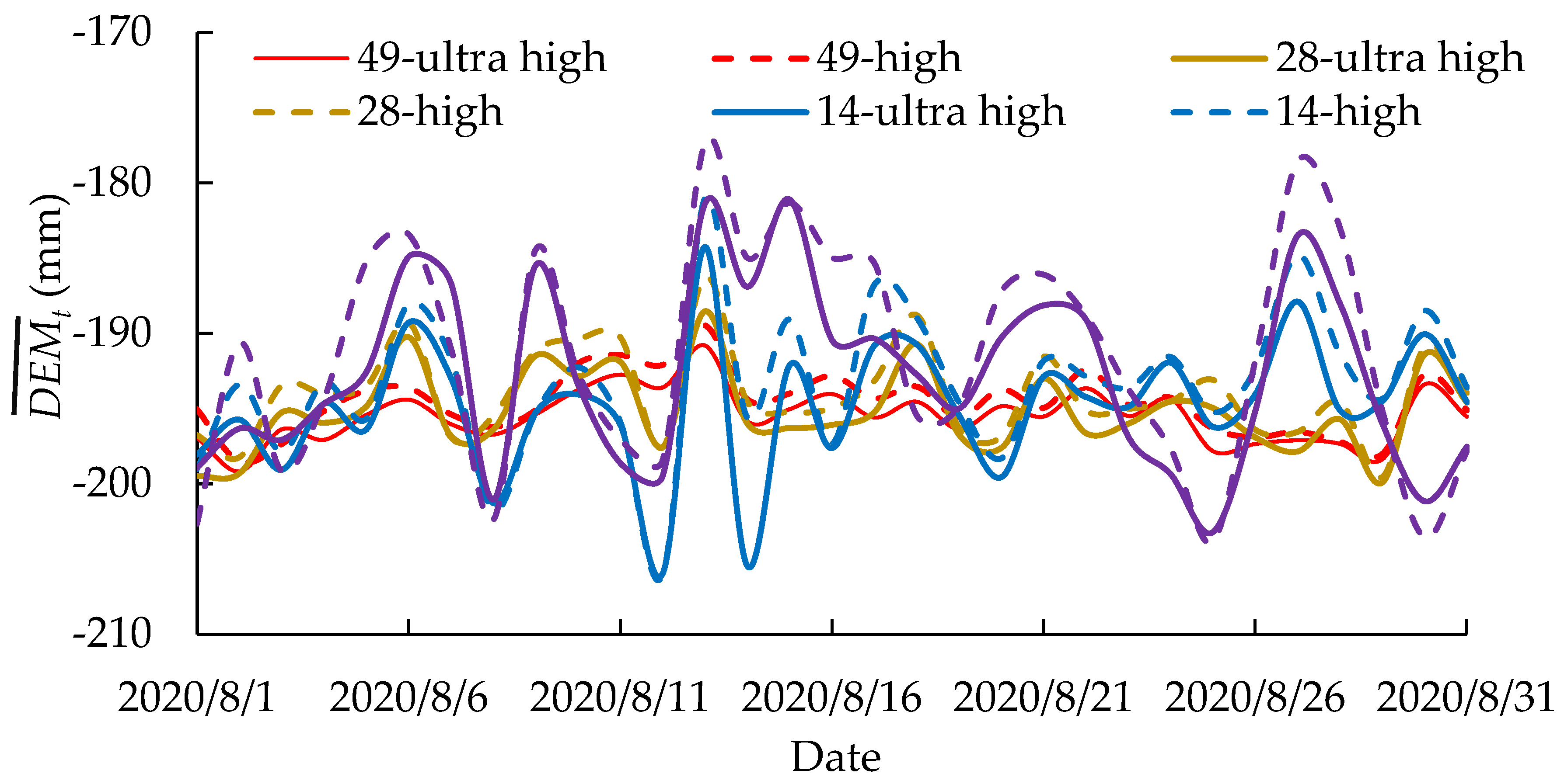
The analysis shows that there are significant differences in the mean values for the DEM data series generated by the 8 4D-SfM models. Especially, the differences caused by the image network geometry are greater than those caused by the processing settings (Figure 4, Table 2). The results in Table 2 show that there are significant differences in the 31-day mean values for the different models. The smaller DEM mean values were obtained when the number of photographs in the image network geometry is higher. The correlation between the DEM mean values for the 8 4D-SfM models in the 31-day time series also shows significant differences (Table 3). When the image network geometries are the same, there is a high correlation between the ultra-high and high processing settings. The correlation coefficients of the model results are significantly lower when the image network geometries are different, regardless of whether the processing settings are the same or not. The analysis shows that the larger the difference in the number of photos between the image network geometry, the lower the correlation coefficient between the 4D-SfM models (Table 3). This indicates that the differences caused by the different image network geometries are greater than those caused by the ultra-high and high processing settings.

3.3. The Stability of the 8 4D-SfM Models

The model with the highest number of photographs combined with the ultra-high processing settings generated the most stable data, and the stability of the model showed a clear trend of decreasing as the number of photographs in the image network geometry decreased (Table 4). As can be seen from Table 4, the absolute deviation and standard deviation measured by the 49-ultra-high model were 1.39 mm and 1.77 mm, respectively, in the dry period. The absolute deviation and standard deviation of 1.31 mm and 1.72 mm were measured by the 49-ultra-high model in the wet period. The ultra-high model has the smallest absolute deviation and standard deviation, which indicates that the model results have the highest stability. When the process settings were the same, the absolute deviation and standard deviation of the model output tended to increase in both dry and wet periods as the photo number for image network geometry decreased. This indicates that the stability of its repeated measurements becomes less stable as the photo number of image network geometry decreases. The absolute deviation and standard deviation of DEMs obtained with ultra-high processing settings are smaller than high processing settings when the image network geometry are the same. It indicates that the stability of DEMs obtained with ultra-high settings is higher than that obtained with high settings.
The difference between the absolute deviation of 49-ultra high and 49-high is 0.18 mm and the difference between the standard deviation is 0.23 mm due to the difference in the processing settings. This indicates that the image network geometry with a large number of photos can significantly reduce the difference between the two different processing settings of ultra high and high. However, when the image network geometry is simple, especially when the number of photos is small such as 7-ultra high and 7 high, the difference caused by the two different processing settings is also increasing. This shows that a reasonable image network geometry can reduce the effect of different processing settings on 4D-SfM data results.

3.4. The Assessment of the Model Accuracy

The 4D-SfM model with the largest number of photos and the ultra-high processing settings has the highest accuracy, and the model accuracy shows an obvious trend of decreasing as the photo number of image network geometry decreases. From Table 5, we can see that the error of the 4D-SfM point cloud model gradually increases with the decrease in the photo number of image network geometry when the processing settings are the same. It can be seen that the model accuracy obtained for the 49-ultra-high model is the highest, with the average difference of −0.56 mm and the absolute error of 1.57 mm. The accuracy of the 28-ultra-high model is slightly lower than that of the 49-ultra model, with the relative error of −0.80 mm and the absolute error of 1.77 mm. When the image network geometries are the same, the accuracy of the model obtained by the ultra-high processing settings is higher than that of the high processing settings (Table 5).

4. Discussion

4.1. Accuracy of 4D-SfM and Other Ground-Based Photogrammetry Studies

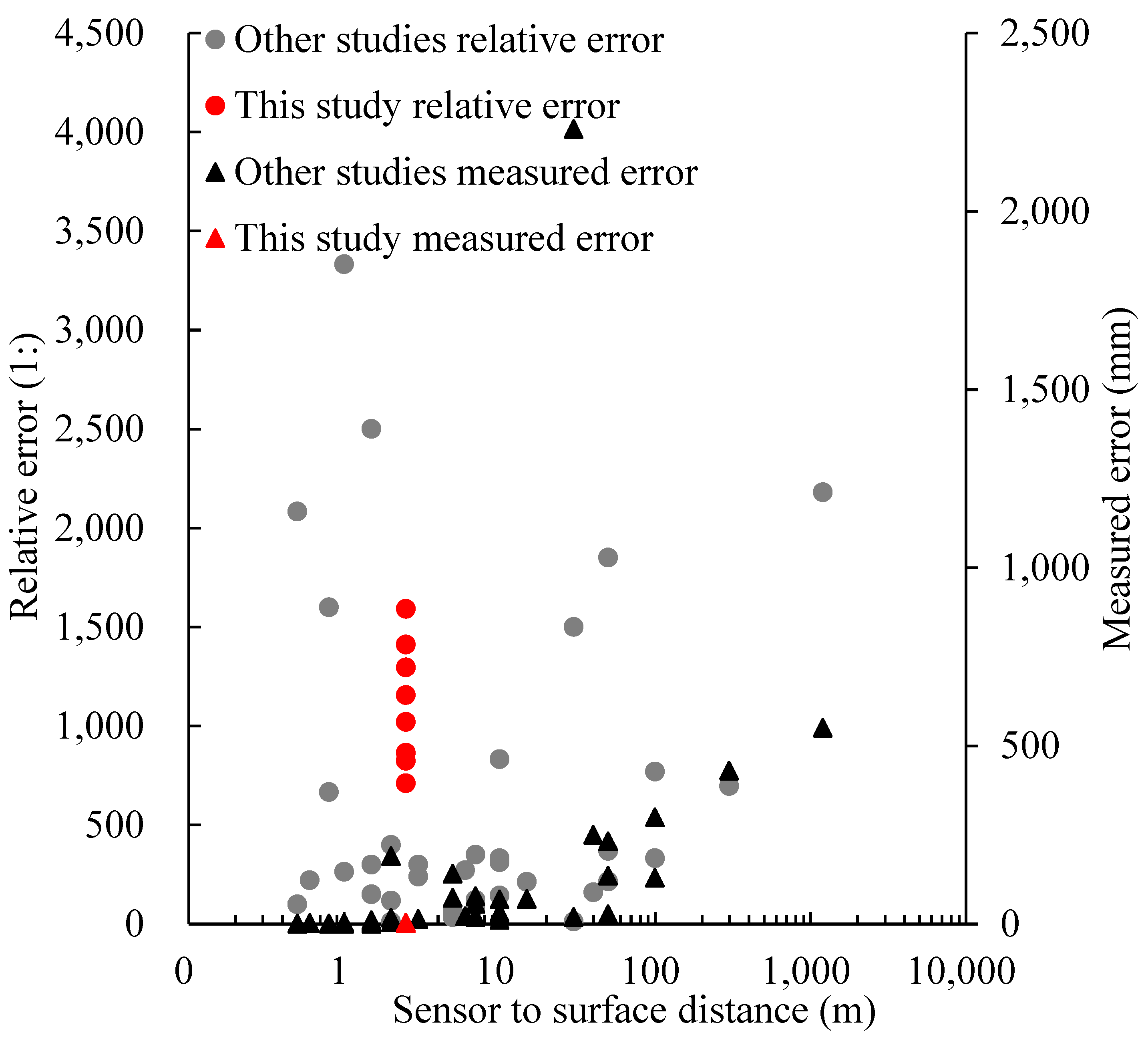
As the difference in set-up for different studies would lead to the results from the different studies being incomparable among them, hence the widely used relative error (measurement precision/observation distance) was used to quantify the accuracy of the SfM photogrammetry of this study to achieve comparable results with other studies. The comparison analysis shows that the relative error of the 4D-SfM data obtained by zigzag image network geometry is smaller than most ground photogrammetry results (Figure 5). According to the results of 24 ground SfM photogrammetry studies (Table 6), the absolute accuracy ranges from 0. 3 mm to 2230 mm, and the relative accuracy ranges from 1:11 to 1:3333. The mean error of this study ranges from −0.56 mm to −2.44 mm and the absolute accuracy of this study ranges from 1.57 mm to 3.51 mm. The relative accuracy ranges from 1:712 to 1:1592. The comparative analysis shows that the relative accuracy of the 49-ultra-high model is better than 85% of all other ground-based photogrammetry models (Table 6).
The relative precision of 4D-SfM photogrammetry from previous studies ranges from 1:13.5 to 1: 1500 [1,25,26,28,36,37]. Compared with previous studies, the relative accuracy of the 49-ultra-high model is 1:1592, which overperformed most of the multi-camera-based 4D-SfM photogrammetry. It indicates the one-camera base 4D-SfM photogrammetry with zigzag-based survey pattern significantly improves ground-based 4D-SfM photogrammetric accuracy.
The 49-ultra high model reaches the highest accuracy. This is mainly due to a number of reasons. At first, the 49-ultra-high model with a zigzag image network geometry has an overlap rate of more than 85% in the front and lateral directions. This image network geometry is more complex and has a higher overlap rate than most of the reported studies in Table 6, so its relative accuracy performance is better. Second, the ultra-high processing settings can greatly increase the number of tie points, which in turn improves the reliability and accuracy of dense clouds and DEM data. In addition, most of the current 4D photogrammetry studies use limited 3 to 15 cameras and obtain fixed camera positions to photograph the measured area. Compared with this study, other 4D photogrammetry studies have not captured as many photos and such a high photo overlap rate as this study [1,25,28]. Moreover, the use of multiple cameras inevitably leads to differences in the intrinsic parameters of each camera, which makes image matching and subsequent processing more challenging. Therefore, the accuracy of the 49-ultra-high and 49-high models in this study is also better than the relative accuracy of multi-camera positions based on 4D-SfM studies [1,25,26,28,36,37].
Table 6. Comparison of this study with other ground-based SfM photogrammetry study performances in measurement error and relative error.
References (Terrestrial)Distance (m)Measurement Error (mm)Relative Error
Castillo et al., 2012 [38]720350.0
Castillo et al., 2014 [39]622273.0
Castillo et al., 2015 [40]1069145.0
Favalli et al., 2012 [41]10.3–3.8367–3333.3
Fonstad et al., 2013 [42]40250160.0
Frankl et al., 2015 [43]217–19010.5, 117.6
Gómez-Gutiérrez et al., 2014 [44]300280, 2101071, 1429
Kaiser et al., 2014 [45]573, 14168.5, 35.5
Leon et al., 2015 [46]1.50.62500.0
Nouwakpo et al., 2015 [47]25400.0
Piermattei et al., 2015 [48]757–30023.3–122.8
Ružić et al., 2014 [49]1570214.0
Smith et al., 2014 [50]50135370.0
Snapir et al., 2014 [51]0.62.7222.0
Stumpf et al. 2014 [20]5027, 2321851.9, 215.5
Rodríguez et al., 2022 [24]0.80.5, 1.21600, 666.7
Morgan, 2019 [23]0.50.242083.3
Eltner et al., 2017 [1]312.5240.0
Gómez-Gutiérrez et al., 2020 [52]1030333.3
Irvine-Fynn et al., 2022 [36]1.55, 10300, 150
He et al., 2022 [5]0.51.8100.0
Chakra et al., 2019 [26]3020, 22301500, 13.5
Filhol et al., 2019 [37]12005502181.8
Liu et al., 2021 [25]314214.3
This study, 49-ultra high2.51.571592.4
This study, 49-high2.52.451020.4
This study, 28-ultra high2.51.771412.4
This study, 28-high2.52.89865.1
This study, 14-ultra high2.51.931295.3
This study, 14-high2.53.03825.1
This study, 7-ultra high2.52.161157.4
This study, 7-high2.53.51712.3
Although the time-lapse 4D-SfM set-up applied in this study has a large advantage in terms of accuracy, it also has a number of problems. The first problem is that the 4D-SfM equipment applied in this study only shoots vertically without titled images. Several studies have proved that survey precision could be improved by the combination of nadir and oblique photogrammetry [53,54,55]. Another problem is that 4D-SfM equipment would take 12 min for the 49 shoots on different positions. During its photographing period, the change in the shadows or the ambient light conditions would lead to the decrease in the matches between the images and the increase in errors [12]. The error can be reduced by shortening the necessary time to capture the picture, and also by increasing the synchronization of the track and camera [25]. Meanwhile, in 4D-SfM photogrammetry, matching ground control points are very time consuming. This would be desirable to develop methods to automatically identify and match ground control points such as template matching [1]. This would allow the more efficient and easy handling of 4D-SfM measurement. In addition, measurement with multiple slides have the problem of track jamming. For long-term measurements, slide lubrication becomes very important.

4.2. The Effect of Surface Conditions on Measurement Accuracy

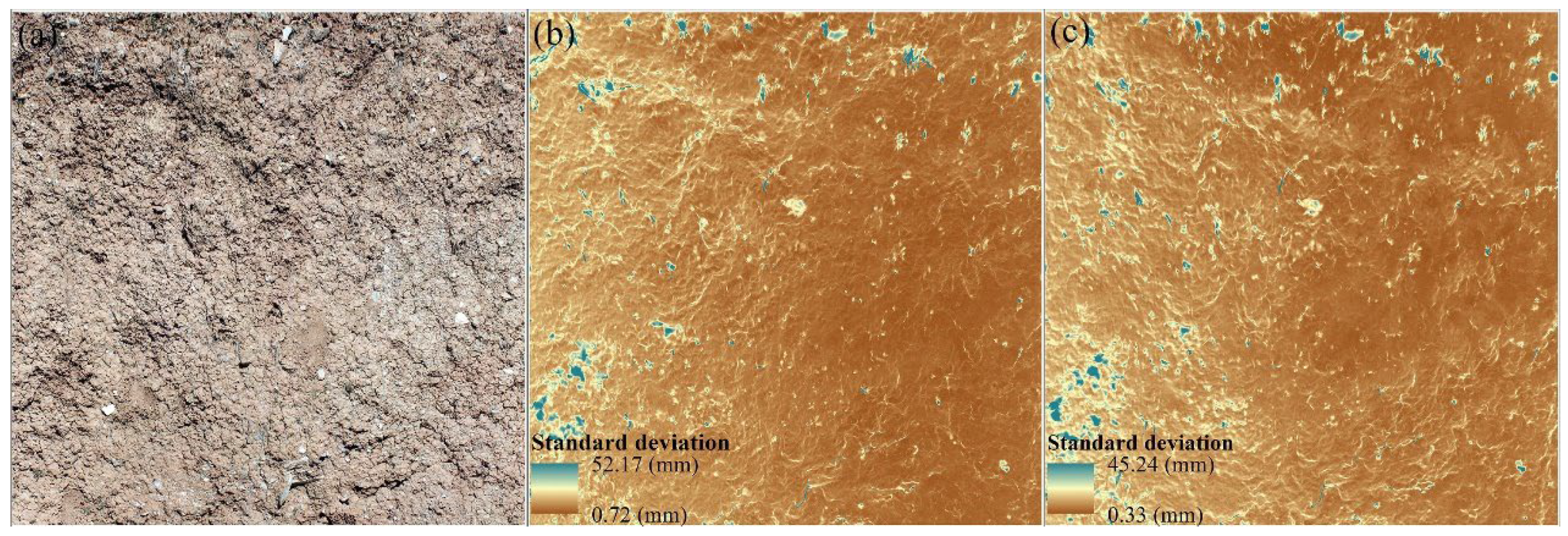
The complexity and surface types of the ground surface are the important factors affecting the measurement accuracy. For this purpose, we calculated the standard deviation of the height (z-axis) of each raster point in dry and wet periods separately using the 49-ultra-high model DEM data. The larger the standard deviation is, the larger the error in the repeated measurements becomes. The influence of surface type on the accuracy of the 4D measurements was also analyzed based on the distribution of features such as surface vegetation, gravel and fissures. For this purpose, we first analyzed the 18-day DEM data for the dry period, and calculated the elevation standard deviation (Figure 6b) for each pixel. It can be seen that the standard deviation of repeated measurements is highest in the porous, soft areas with large surface microtopography, up to 52.2 mm, followed by higher standard deviation in the areas with vegetation cover. When the surface was wet after rainfall, the standard deviation distribution calculated using the 13 days DEM data was similar to that of the dry period, but the overall standard deviation was smaller than that of the dry period (Figure 6c). It means the 4D-SfM models performed slightly better on the wet days than on the dry days.
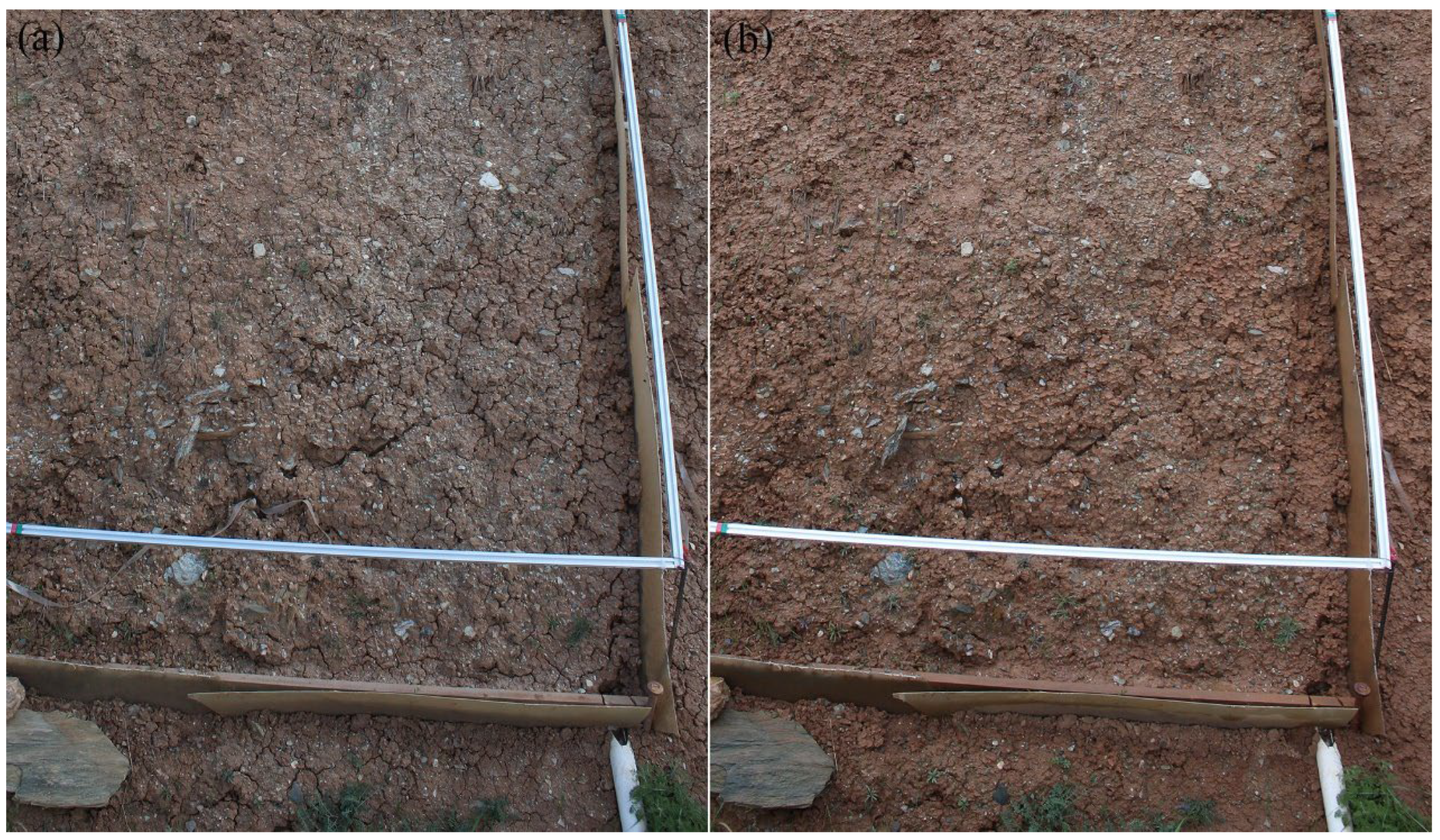
With different soil surface characteristics during the wet and dry periods, it can be seen that during the dry period, fissures are developed in the study plot (Figure 7a). While during the wet period, fissures are reduced due to soil expansion (Figure 7b). The dry period with fissure development is not conducive to high-precision photogrammetry which could reduce its precision more in the dry period than in the wet period. At the same time, we compared the differences between the photographs captured during the dry and wet periods. We found that the quality of the photographs captured on wet days is more superior than those captured on dry days. The surface characteristics of the dry bare slope show more complex characteristics compared with the wet days, which is not conducive to high-precision photogrammetry. The above-mentioned multiple factors are responsible for the higher accuracy of the 4D-SfM data in wet periods than in dry soil periods. Since the rainfall was the main factor which induces soil wetness, it means that rainfall can indirectly affect the results of the field 4D-SfM measurement precision by changing its bare slope surface conditions.

4.3. The Potential Application of 4D-SfM

The high accuracy of 4D-SfM photogrammetry in the field measurement indicates that the small change in surface process can be observed with 4D-SfM. For example, snow-surface sublimation is the main pathway for lake ice, glacier and snow cover loss in winter. The reported sublimation rates fluctuated by around 0.05 to 2.4 mm/day [56,57,58,59]. If 4D-SfM photogrammetry achieves a sub-millimeter accuracy in a vertical direction, then such complex processes can be captured using 4D photogrammetry. The studies on soil wet and dry changes due to surface rainfall, slope erosion and gully erosion are difficult to observe continuously outdoors for long periods of time because of the high accuracy required for observation. Currently, we mainly rely on indoor photographic measurements to quantify the spatial distribution of erosion volume. If field high-precision (sub-millimeter) 4D-SfM measurements can be widely applied, it will be helpful for observational studies on snow surface, ice sublimation and rainfall erosion. Future attempts can be made to utilize single-camera zigzag shooting combined with a focused survey mode, which may further improve the accuracy of 4D-SfM photogrammetry.

5. Conclusions

Different image network geometry as well as the processing settings have a significant impact on the model reconstruction results. As the image network geometry becomes simpler, the differences between the two processing settings on the model results increase. A reasonable image network geometry (such as the 49-ultra-high model) can effectively reduce the difference between different processing settings.
The 49-ultra-high model has the highest stability and accuracy, but it is the most time consuming. As the number of photos decreases, the accuracy and stability of the 4D-SfM model decrease. It can be seen that the 49-ultra-high model is recommended for high accuracy, and the 49-high model is recommended when the processing time cost is the primary consideration. The increase in the repetition of lateral and forward directions with multi-angle shots can greatly help to improve 4D-SfM model accuracy and stability in field ground-based photogrammetry. In particular, the relative accuracy of a zigzag survey pattern (such as the 49-ultra-high model) is superior to 85% of all focused survey patterns.
The measurement error is relevant to the ground complexity. The 4D-SfM models errors are high for surface types with loose and undulating ground surfaces. The measurement error is also relatively high for the surface covered with vegetation. Thus, we suggest that if there is vegetation in the study area, early weeding is recommended. The higher accuracy of bare ground 4D-SfM models during the wet time relative to the dry time period may be strongly related to the higher quality of photographs captured during the wet time and the swelling of a clay-induced reduction in ground fissures. It is clear that the best time to carry out outdoor bare ground (clay ground) photogrammetry is when the soil is wet and the weather is cloudy.

Author Contributions

J.L.: conceptualization, methodology, methodology, writing—original draft and review, data acquisition and tests. S.M.: formal analysis and writing—review. R.C.: funding acquisition, data acquisition and conceptualization. All authors have read and agreed to the published version of the manuscript.

Funding

This work was supported by the National Natural Science Foundation of China (Grant No. 42271154, 41877163), the “Hundred Talent Program” of the Chinese Academy of Sciences (Y729G01002), and the Science and Technology National Key Research and Development Project of China (2019YFC1510504).

Data Availability Statement

The data are available by contacting the author of Junfeng Liu.

Conflicts of Interest

The authors declare no conflict of interest.

References

  1. Eltner, A.; Kaiser, A.; Abellan, A.; Schindewolf, M. Time lapse structure-from-motion photogrammetry for continuous geomorphic monitoring. Earth Surf. Process. Landf. 2017, 42, 2240–2253. [Google Scholar] [CrossRef]
  2. Ryan, J.C.; Hubbard, A.L.; Box, J.E.; Todd, J.; Christoffersen, P.; Carr, J.R.; Holt, T.; Snooke, N. UAV photogrammetry and structure from motion to assess calving dynamics at store glacier, a large outlet draining the Greenland ice sheet. Cryosphere 2015, 9, 1–11. [Google Scholar] [CrossRef] [Green Version]
  3. Revuelto, J.; López-Moreno, J.I.; Alonso-González, E. Light and shadow in mapping alpine snowpack with unmanned aerial vehicles in the absence of ground control points. Water Resour. Res. 2021, 57, e2020WR028980. [Google Scholar] [CrossRef]
  4. Gomez, C.; Hayakawa, Y.; Obanawa, H. A study of Japanese landscapes using structure from motion derived DSMs and DEMs based on historical aerial photographs: New opportunities for vegetation monitoring and diachronic geomorphology. Geomorphology 2015, 242, 11–20. [Google Scholar] [CrossRef] [Green Version]
  5. He, T.; Yang, Y.; Shi, Y.; Liang, X.; Fu, S.; Xie, G.; Liu, B.; Liu, Y. Quantifying spatial distribution of interrill and rill erosion in a loess at different slopes using structure from motion (SfM) photogrammetry. Int. Soil Water Conserv. Res. 2022, 10, 393–406. [Google Scholar] [CrossRef]
  6. Bendig, J.; Bolten, A.; Bennertz, S.; Broscheit, J.; Eichfuss, S.; Bareth, G. Estimating biomass of barley using crop surface models (CSMs) derived from UAV-based RGB imaging. Remote Sens. 2014, 6, 10395–10412. [Google Scholar] [CrossRef] [Green Version]
  7. Cunliffe, A.; Anderson, K. Measuring above-Ground Biomass with Drone Photogrammetry: Data Collection Protocol, 2 January 2019, PROTOCOL (Version 1). Protocol Exchange. Available online: https://www.researchgate.net/publication/330096533_Measuring_Above-ground_Biomass_with_Drone_Photogrammetry_Data_Collection_Protocol (accessed on 22 April 2023).
  8. Cunliffe, A.M.; Anderson, K.; Boschetti, F.; Brazier, R.E.; Graham, H.A.; Myers-Smith, I.H.; Astor, T.; Boer, M.M.; Calvo, L.G.; Clark, P.E.; et al. Global application of an unoccupied aerial vehicle photogrammetry protocol for predicting above ground biomass in non-forest ecosystems. Remote Sens. Ecol. Conserv. 2022, 8, 57–71. [Google Scholar] [CrossRef]
  9. Forsmoo, J.; Anderson, K.; Macleod, C.J.A.; Wilkinson, M.E.; Brazier, R. Drone-based structure-from-motion photogrammetry captures grassland sward height variability. J. Appl. Ecol. 2018, 55, 2587–2599. [Google Scholar] [CrossRef]
  10. Iglhaut, J.; Cabo, C.; Puliti, S.; Piermattei, L.; O’Connor, J.; Rosette, J. Structure from Motion photogrammetry in forestry: A review. Curr. For. Rep. 2019, 5, 155–168. [Google Scholar] [CrossRef] [Green Version]
  11. Eltner, A.; Sofia, G. Structure from motion photogrammetric technique, 1st ed. In Developments in Earth Surface Processes; Elsevier: Amsterdam, The Netherlands, 2020; Volume 23, pp. 1–22. [Google Scholar]
  12. Eltner, A.; Kaiser, A.; Castillo, C.; Rock, G.; Neugirg, F.; Abellan, A. Image-based surface reconstruction in geomorphometry—Merits, limits and developments. Earth Surf. Dynam. 2016, 4, 359–389. [Google Scholar] [CrossRef] [Green Version]
  13. Smith, M.W.; Carrivick, J.L.; Quincey, D.J. Structure from motion photogrammetry in physical geography. Prog. Phys. Geogr. 2016, 40, 247–275. [Google Scholar] [CrossRef] [Green Version]
  14. James, M.; Chandler, J.; Eltner, A.; Fraser, C.; Miller, P.; Mills, J.; Noble, T.; Robson, S.; Lane, S. Guidelines on the use of structure from motion photogrammetry in geomorphic research. Earth Surf. Process. Landf. 2019, 44, 2081–2084. [Google Scholar] [CrossRef]
  15. Westoby, M.J.J.; Brasington, J.; Glasser, N.F.F.; Hambrey, M.J.J.; Reynolds, J.M.M. “Structure-from-motion” photogrammetry: A low-cost, effective tool for geoscience applications. Geomorphology 2012, 179, 300–314. [Google Scholar] [CrossRef] [Green Version]
  16. Griffiths, D.; Burningham, H. Comparison of pre- and selfcalibrated camera calibration models for UAS-derived nadir imagery for a SfM application. Prog. Phys. Geogr. 2019, 43, 215–235. [Google Scholar] [CrossRef] [Green Version]
  17. James, M.R.; Robson, S. Sequential digital elevation models of active lava flows from ground-based stereo time-lapse imagery. ISPRS J. Photogramm. Remote Sens. 2014, 97, 160–170. [Google Scholar] [CrossRef]
  18. James, M.R.; Robson, S. Straightforward reconstruction of 3-D surfaces and topography with a camera: Accuracy and geoscience application. J. Geophys. Res. 2012, 117, F03017. [Google Scholar] [CrossRef] [Green Version]
  19. Senn, J.A.; Mills, J.; Walsh, C.L.; Addy, S.; Peppa, M. On-site geometric calibration of RPAS mounted sensors for SfM photogrammetric geomorphological surveys. Earth Surf. Process. Landf. 2022, 47, 1615–1634. [Google Scholar] [CrossRef]
  20. Stumpf, A.; Malet, J.-P.; Allemand, P.; Pierrot-Deseilligny, M.; Skupinski, G. Ground-based multi-view photogrammetry for the monitoring of landslide deformation and erosion. Geomorphology 2014, 231, 130–145. [Google Scholar] [CrossRef]
  21. Gaiani, M.; Remondino, F.; Apollonio, F.I.; Ballabeni, A. An advanced pre-processing pipeline to improve automated photogrammetric reconstructions of Architectural scenes. Remote Sens. 2016, 8, 178. [Google Scholar] [CrossRef] [Green Version]
  22. Forsmoo, J.; Anderson, K.; Macleod, C.J.A.; Wilkinson, M.E.; BeBell, L.; Brazier, R. Structure from motion photogrammetry in ecology: Does the choice of software matter? Ecol. Evol. 2019, 9, 12964–12979. [Google Scholar] [CrossRef]
  23. Morgan, B.; Ford, A.L.J.; Smith, M.J. Standard methods for creating digital skeletal models using structure-from-motion photogrammetry. Am. J. Phys. Anthropol. 2019, 169, 152–160. [Google Scholar] [CrossRef] [PubMed]
  24. Rodríguez, R.F.; Ponte, M.; Bento, R.; Cardoso, R. Potential of mobile application based on structure from motion (SfM) photogrammetry to monitor slope fast erosion by runoff water. Catena 2022, 216, 106359. [Google Scholar] [CrossRef]
  25. Liu, J.; Chen, R.; Ding, Y.; Han, C.; Ma, S. Snow process monitoring using time-lapse structure-from-motion photogrammetry with a single camera. Cold Reg. Sci. Technol. 2021, 190, 103355. [Google Scholar] [CrossRef]
  26. Chakra, C.A.; Gascoin, S.; Somma, J.; Fanise, P.; Drapeau, L. Monitoring the snowpack volume in a Sinkhole on Mount Lebanon using time lapse photogrammetry. Sensors 2019, 19, 3890. [Google Scholar] [CrossRef] [Green Version]
  27. James, M.R.; Robson, S. Mitigating systematic error in topographic models derived from UAV and ground-based image networks. Earth Surf. Process. Landf. 2014, 39, 1413–1420. [Google Scholar] [CrossRef] [Green Version]
  28. Mallalieu, J.; Carrivick, J.L.; Quincey, D.J.; Smith, M.W.; James, W.H.M. An integrated structure-from-motion and time-lapse technique for quantifying ice-margin dynamics. J. Glaciol. 2017, 63, 937–949. [Google Scholar] [CrossRef] [Green Version]
  29. Galland, O.; Bertelsen, H.S.; Guldstrand, F.; Girod, L.; Johannessen, R.F.; Bjugger, F.; Burchardt, S.; Mair, K. Application of open-source photogrammetric software MicMac for monitoring surface deformation in laboratory models. J. Geophys. Res. Solid Earth 2016, 121, 2852–2872. [Google Scholar] [CrossRef] [Green Version]
  30. Young, D.J.N.; Koontz, M.J.; Weeks, J. Optimizing aerial imagery collection and processing parameters for drone-based individual tree mapping in structurally complex conifer forests. Methods Ecol. Evol. 2022, 13, 1447–1463. [Google Scholar] [CrossRef]
  31. Gerke, M.; Przybilla, H. Accuracy analysis of photogrammetric UAV image blocks: Influence of on board RTK-GNSS and cross flight patterns. Photogramm. Fernerkund. Geoinf. 2016, 17–30. [Google Scholar] [CrossRef] [Green Version]
  32. Bayley, D.T.I.; Mogg, A.O.M. A protocol for the large-scale analysis of reefs using structure from Motion photogrammetry. Methods Ecol. Evol. 2020, 11, 1410–1420. [Google Scholar] [CrossRef]
  33. Agisoft, LLC. PhotoScan User Manual, Professional Edition, Version 1.4. 2008. Available online: https://www.agisoft.com/pdf/photoscan-pro_1_4_en.pdf (accessed on 22 April 2023).
  34. Deliry, S.I.; Avdan, U. Accuracy of Unmanned Aerial Systems Photogrammetry and Structure from Motion in Surveying and Mapping: A Review. J. Indian Soc. Remote Sens. 2021, 49, 1997–2017. [Google Scholar] [CrossRef]
  35. Morel, J.M.; Yu, G. ASIFT: A new framework for fully affine invariant image comparison. SIAM J. Imaging Sci. 2009, 2, 438–469. [Google Scholar] [CrossRef] [Green Version]
  36. Irvine-Fynn, T.D.L.; Holt, T.O.; James, T.D.; Smith, M.W.; Rutter, N.; Porter, P.R.; Hodson, A.J. Time-lapse photogrammetry reveals hydrological controls of fine-scale High-Arctic glacier surface roughness evolution. Earth Surf. Process. Landf. 2022, 47, 1635–1652. [Google Scholar] [CrossRef]
  37. Filhol, S.; Perret, A.; Girod, L.; Sutter, G.; Schuler, T.V.; Burkhart, J.F. Time-Lapse Photogrammetry of distributed snow depth during snowmelt. Water Resour. Res. 2019, 55, 7916–7926. [Google Scholar] [CrossRef] [Green Version]
  38. Castillo, C.; James, M.R.; Redel-Macías, M.D.; Pérez, R.; Gómez, J.A. SF3M software: 3-D photo-reconstruction for nonexpert users and its application to a gully network. Soil 2015, 1, 583–594. [Google Scholar] [CrossRef] [Green Version]
  39. Castillo, C.; Pérez, R.; James, M.R.; Quinton, J.N.; Taguas, E.V.; Gómez, J.A. Comparing the Accuracy of Several Field Methods for Measuring Gully Erosion. Soil Sci. Soc. Am. J. 2012, 76, 1319–1332. [Google Scholar] [CrossRef] [Green Version]
  40. Castillo, C.; Taguas, E.V.; Zarco-Tejada, P.; James, M.R.; Gómez, J.A. The normalized topographic method: An automated procedure for gully mapping using GIS. Earth Surf. Process. Landf. 2014, 39, 2002–2015. [Google Scholar] [CrossRef]
  41. Favalli, M.; Fornaciai, A.; Isola, I.; Tarquini, S.; Nannipieri, L. Multiview 3-D reconstruction in geosciences. Comput. Geosci. 2012, 44, 168–176. [Google Scholar] [CrossRef] [Green Version]
  42. Fonstad, M.A.; Dietrich, J.T.; Courville, B.C.; Jensen, J.L.; Carbonneau, P.E. Topographic structure from motion: A new development in photogrammetric measurement. Earth Surf. Process. Landf. 2013, 38, 421–430. [Google Scholar] [CrossRef] [Green Version]
  43. Frankl, A.; Stal, C.; Abraha, A.; Nyssen, J.; Rieke-Zapp, D.; De Wulf, A.; Poesen, J. Detailed recording of gully morphology in 3-D through image-based modelling PhotoScan Digital Elevation Model (DEM) Soil pipes Structure from M otion–Multi View Stereo (SfM–MVS) Volume calculation. Catena 2015, 127, 92–101. [Google Scholar] [CrossRef] [Green Version]
  44. Gómez-Gutiérrez, Á.; de Sanjosé-Blasco, J.J.; de Matías Bejarano, J.; Berenguer-Sempere, F. Comparing Two Photo Reconstruction Methods to Produce High Density Point Clouds and DEMs in the Corral del Veleta Rock Glacier (Sierra Nevada, Spain). Remote Sens. 2014, 6, 5407–5427. [Google Scholar] [CrossRef] [Green Version]
  45. Kaiser, A.; Neugirg, F.; Rock, G.; Müller, C.; Haas, F.; Ries, J.; Schmidt, J. Small-Scale Surface Reconstruction and Volume Calculation of Soil Erosion in Complex Moroccan Gully Morphology Using Structure from Motion. Remote Sens. 2014, 6, 7050–7080. [Google Scholar] [CrossRef] [Green Version]
  46. Leon, J.X.; Roelfsema, C.M.; Saunders, M.I.; Phinn, S.R. Measuring coral reef terrain roughness using “Structure-from-Motion” close-range photogrammetry. Geomorphology 2015, 242, 21–28. [Google Scholar] [CrossRef]
  47. Nouwakpo, S.K.; James, M.R.; Weltz, M.A.; Huang, C.-H.; Chagas, I.; Lima, L. Evaluation of structure from motion for soil microtopography measurement. Photogramm. Rec. 2014, 29, 297–316. [Google Scholar] [CrossRef]
  48. Piermattei, L.; Carturan, L.; Guarnieri, A. Use of terrestrial photogrammetry based on structure from motion for mass balance estimation of a small glacier in the Italian Alps. Earth Surf. Process. Landf. 2015, 40, 1791–1802. [Google Scholar] [CrossRef]
  49. Ružić, I.; Marovic, I.; Benac, C.; Ilic, S. Coastal cliff geometry derived from structure-from-motion photogrammetry at Stara Baka, Krk Island, Croatia. Geo Mar. Lett. 2014, 34, 555–565. [Google Scholar] [CrossRef]
  50. Smith, M.W.; Carrivick, J.L.; Hooke, J.; Kirkby, M.J. Reconstructing flash flood magnitudes using “Structure-from-Motion”: A rapid assessment tool. J. Hydrol. 2014, 519, 1914–1927. [Google Scholar] [CrossRef]
  51. Snapir, B.; Hobbs, S.; Waine, T.W. Roughness measurements over an agricultural soil surface with Structure from Motion. ISPRS J. Photogramm. Remote Sens. 2014, 96, 210–223. [Google Scholar] [CrossRef]
  52. Gómez-Gutiérrez, Á.; Biggs, T.; Gudino-Elizondo, N.; Errea, P.; Alonso-González, E.; Nadal Romero, E.; de Sanjosé Blasco, J. Using visibility analysis to improve point density and processing time of SfM-MVS techniques for 3D reconstruction of landforms. Earth Surf. Process. Landf. 2020, 45, 2524–2539. [Google Scholar] [CrossRef]
  53. James, M.R.; Robson, S.; Smith, M.W. 3-D uncertainty-based topographic change detection with structure-from-motion photogrammetry: Precision maps for ground control and directly georeferenced surveys. Earth Surf. Process. Landf. 2017, 42, 1769–1788. [Google Scholar] [CrossRef]
  54. Agueera-Vega, F.; Carvajal-Ramirez, F.; Martinez-Carricondo, P.; López, J.S.; Mesas-Carrascosa, F.J.; Garcia-Ferrer, A.; Pérez-Porras, F.J. Reconstruction of extreme topography from UAV structure from motion photogrammetry. Measurement 2018, 121, 127–138. [Google Scholar] [CrossRef]
  55. Rusnák, M.; Sládek, J.; Kidová, A.; Lehotský, M. Template for high-resolution river landscape mapping using UAV technology. Measurement 2018, 115, 139–151. [Google Scholar] [CrossRef]
  56. Hood, E.; Williams, M.; Cline, D. Sublimation from a seasonal snowpack at a continental, mid-latitude alpine site. Hydrol. Process. 1999, 13, 1781–1797. [Google Scholar] [CrossRef]
  57. Marks, D.; Dozier, J. Climate and energy exchanges at the snow surface in the alpine region of the Sierra Nevada: 2. Snow cover energy balance. Water Resour. Res. 1992, 28, 3043–3054. [Google Scholar] [CrossRef]
  58. Stössel, F.; Guala, M.; Fierz, C.; Manes, C.; Lehning, M. Micrometeorological and morphological observations of surface hoar dynamics on a mountain snow cover. Water Resour. Res. 2010, 46, 1–11. [Google Scholar] [CrossRef] [Green Version]
  59. Li, S.; Yao, T.; Yang, W.; Yu, W.; Zhu, M. Glacier energy and mass balance in the inland Tibetan Plateau: Seasonal and interannual variability in relation to atmospheric changes. J. Geophys. Res. Atmos. 2018, 123, 6390–6490. [Google Scholar] [CrossRef]
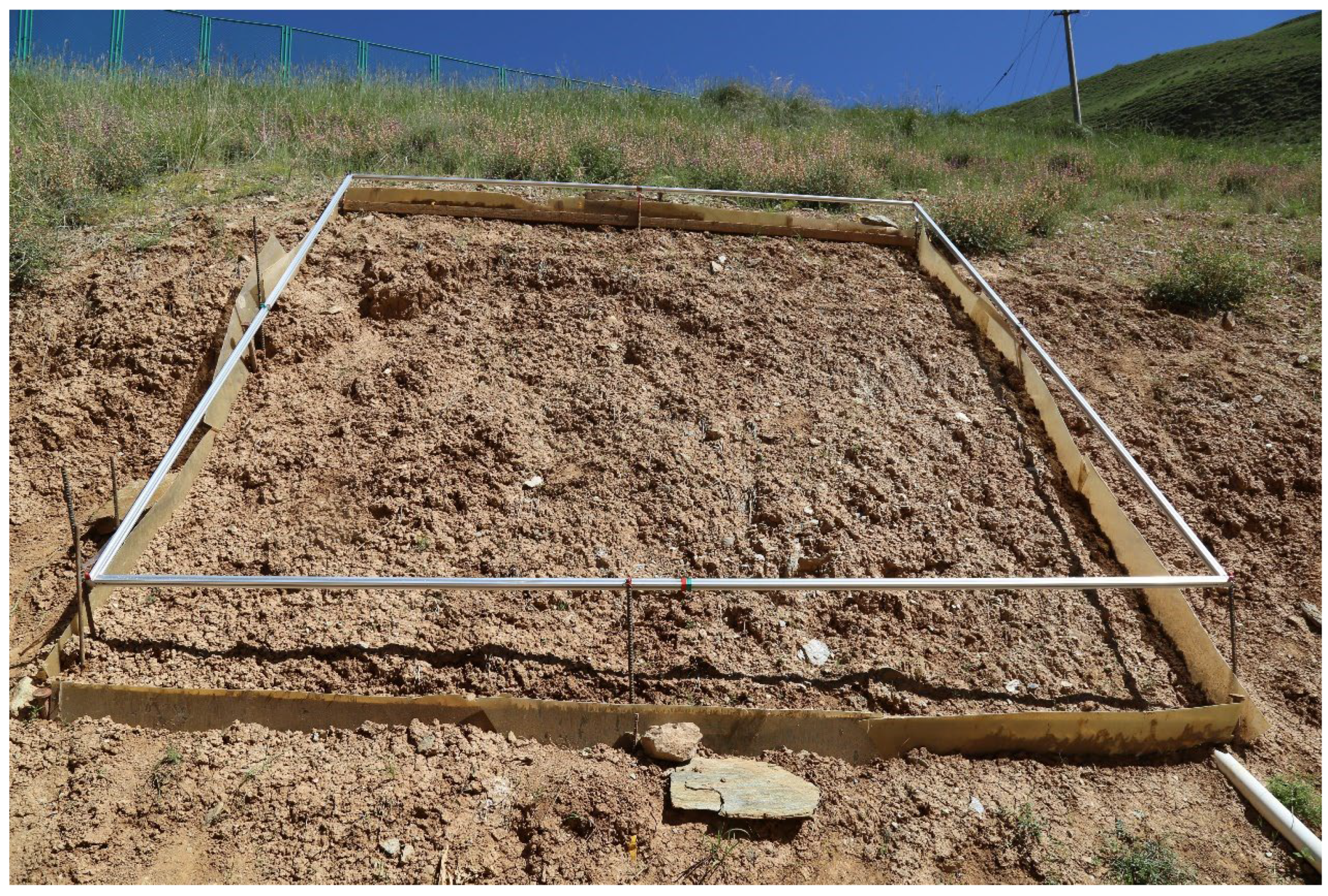
Figure 1. Test site overview.
Remotesensing 15 02269 g001
Figure 2. Schematic plot of the time-lapse 4D-SfM photogrammetry experimental apparatus. (1) Canon EOS 1100D camera; (2) 2A, 2B and 2C are three 1.5 m long ball-bearing lead screws; (3) scaffold; (4) 4 × 4 × 0.1 m aluminum frame used as control frame; (5) eight ground control points distributed on the aluminum frame. Four GCPs located at four corners of the frame, four GCPs located in middle of the 4 m long stakes.
Remotesensing 15 02269 g002
Figure 3. Four different image network geometries. Image network geometry 1 applied all the 49 photos in the mode, in which all pictures evenly distributed over 1.5 × 1.5 m squares. The arrow in image network geometry 1 stands for the movement of camera. The image network geometry 2 reduced the frontal directional pictures overlap to 28 pictures. The image network geometry 3 further reduced the pictures to 14. The image network geometry 4 reduced the pictures to 7 which indicates we only include the lateral overlaps.
Remotesensing 15 02269 g003
Figure 4. Variation in the time-lapse 4D-SfM set-up derived from 8 models (mean of DEMs over 31 days).
Remotesensing 15 02269 g004
Figure 5. The comparison of this study’s 8 4D-SfM measured models and relative error with other studies.
Remotesensing 15 02269 g005
Figure 6. (a) Study plot orthoimage; (b) standard deviation of measured 18 DEMs by O-T-SfM photogrammetry on dry days; (c) standard deviation of measure 13 DEMs by O-T-SfM photogrammetry on wet days.
Remotesensing 15 02269 g006
Figure 7. (a) Picture captured by time-lapse 4D-SfM photogrammetry camera on 29 August when the plot was dry and fissures were scattered over the bare soil surface; (b) picture captured by time-lapse 4D-SfM camera on next day after a 7.5 mm rainfall, the swell of soil induced the disappearance of the fissures.
Remotesensing 15 02269 g007
Table 1. The tie points, dense cloud and consumed time of the 8 4D-SfM models.
ModelTie PointsDense Cloud NumberTime Consumed (h)Overlap at Front Direction Overlap at Lateral Direction
49-ultra high90404.50 × 10710.585%85%
49-high84301.03 × 1076.485%85%
28-ultra high59873.63 × 1074.3280%85%
28-high58468.19 × 1062.2180%85%
14-ultra high59873.63 × 1071.3270%85%
14-high58468.19 × 1060.2170%85%
7-ultra high57403.20 × 1070.33085%
7-high56507.21 × 1060.12085%
Table 2. The 31-day mean values for the 8 4D-SfM models.
Mode49-Ultra High49-High28-Ultra High28-High14-Ultra High14-High7-Ultra High7-High
D E M ¯ (mm)−195.50−194.61−195.19−194.01−194.88−193.29−192.75−191.38
Table 3. Correlation coefficients between 8 model’s D E M ¯ t over 31 days.
49-Ultra High49-High28-Ultra High28-High14-Ultra High14-High7-Ultra High7-High
49-ultra high1.00
49-high0.961.00
28-ultra high0.680.601.00
28-high0.650.610.971.00
14-ultra high0.240.170.470.481.00
14-high0.210.160.490.490.921.00
7-ultra high0.230.210.230.230.410.561.00
7-high0.180.170.170.170.370.530.931
Table 4. Mean of selected DEMs on dry and wet days, absolute bias and standard deviation of 8 4D-SfM models on dry and wet days.
Dry/Wet DaysModel D E M ¯ (mm) Abs (mm)Std (mm)
Dry49-ultra high−195.491.391.77
49-high−194.481.592.02
28-ultra high−195.961.642.36
28-high−194.811.942.76
14-ultra high−195.063.434.89
14-high−193.173.805.23
7-ultra high−191.195.156.09
7-high−190.136.457.49
Wet49-ultra high−195.521.311.72
49-high−194.861.481.93
28-ultra high−193.792.542.80
28-high−192.562.442.79
14-ultra high−194.542.773.51
14-high−193.493.083.97
7-ultra high−194.274.715.54
7-high−193.665.466.58
Table 5. Mean error, absolute error between the physical measurements and the model estimates for 8 models.
ModelMean Error (mm)Absolute Error (mm)RMSE (mm)
49-ultra high−0.561.572.01
49-high−1.552.453.14
28-ultra high−0.801.772.41
28-high−2.212.893.80
14-ultra high−1.141.932.52
14-high−1.893.034.03
7-ultra high−1.242.162.94
7-high−2.443.514.86
Disclaimer/Publisher’s Note: The statements, opinions and data contained in all publications are solely those of the individual author(s) and contributor(s) and not of MDPI and/or the editor(s). MDPI and/or the editor(s) disclaim responsibility for any injury to people or property resulting from any ideas, methods, instructions or products referred to in the content.