Characterization and Evaluation of Thaw-Slumping Using GPR Attributes in the Qinghai–Tibet Plateau

Simple Summary

Global warming and engineering construction have had an impact on the melting of permafrost on both sides of the Qinghai–Tibet Project Corridor. Due to changes in the internal moisture content of slopes after thawing of frozen soil, thaw-slumping often occur in slope areas. The GPR data type carries the geometric distribution and physical property information of the internal medium of the landslide. By utilizing GPR multi–attribute calculation and analysis, more precise distribution characteristics of the internal layers and relative water content of thaw-slumping can be quickly obtained. These data can provide support for the characterization and evaluation of thaw-slumping.

Abstract

Due to the impact of climate warming and engineering construction, thaw-slumping has developed extensively along the Qinghai–Tibet Project Corridor. These landslide disasters not only destroy the fragile ecology of the Qinghai–Tibet Plateau but also threaten the security of the Qinghai–Tibet Project Corridor. Because remote-sensing images lack imaging data inside the landslide body, and the excavation of boreholes has blindness and inefficiency, the ground-penetrating radar method with high efficiency and deep imaging has been developed and applied in the detection and treatment of thaw-slumping. To more accurately divide the soil-layered structure of the thaw-slumping body and obtain the key elements of the thaw-slumping such as temperature change trend and relative water content, we propose the use of amplitude event axis tracking and amplitude energy attenuation calculation to divide the fine layering of the thaw-slumping body. In addition, based on layer division, we introduce two attribute parameters to participate in the calculation of relative water content. These two attribute parameters are the weighted average frequency attribute, which reflects the temperature change trend, and the sweetness attribute, which reflects the change in the physical properties of the underground medium. The calculated 3D profile and time slice of the relative water content comprehensively show the change characteristics and enrichment area of the internal relative water content of the thaw-slumping. These methods and results are valuable for the characterization, evaluation, and treatment of thaw-slumping.

1. Introduction

The Qinghai–Tibet Plateau (QTP)’s higher altitude and harsh climatic conditions have developed frozen soil with the largest area, the highest altitude, and the widest distribution in the middle and low latitudes of the world [1,2]. Frozen soil on the Qinghai–Tibet Plateau refers to various rocks and soils containing ice below 0 °C. It generally can be divided into short-term frozen soil (several hours/days or even half a month), seasonally frozen soil (half a month to several months), and permafrost (a few years to tens of thousands of years). These frozen soils have relatively poor thermal stability due to their large ice content, increased temperature, and low thickness on the Qinghai–Tibet Plateau [3,4]. Due to the sensitivity of seasonally frozen soil to temperature, from June to September each year, the increase in temperature causes the ablation of frozen soil. As the global temperature continues to rise, the depth of ablation of seasonally frozen soil continues to increase on large scales, and the temperature and water content inside the frozen soil gradually increase. On small scales, especially in the Qinghai–Tibet Project Corridor, the degradation of frozen soil caused by human engineering activities is often greater than climate change [5,6]. With the deterioration of frozen soil and the increase of engineering activities, thermal-thawing disasters continue to occur along the Qinghai–Tibet Project Corridor. These thermal-thawing disasters mainly manifest as shallow frozen soil landslides, thaw-slumping, and thermal-thawing debris flow [7]. As of 2015, field survey work and remote-sensing image data show that a total of 42 thaw-slumping and landslides have been found within 10 km (from Fenghuoshan section to Chumar River) along the sides of the Qinghai–Tibet Railway embankment. Among them, 12 are distributed within 52 km of Hoh Xil Mountain, 24 are distributed within 21 km of Beiluhe Basin, and six are distributed within 19.5 km of Fenghuoshan Mountain [8]. Since thaw-slumping is often distributed near railways, highways, and other construction projects, it poses a potential threat to the frozen soil environment and existing engineering facilities, and as the scale of engineering construction gradually increases, the frequency and scale of thermal melt disasters in the corridor will also gradually increase [9]. Therefore, studying the permafrost thaw-slumping developed on both sides of the Qinghai–Tibet Plateau Engineering Corridor has good value for engineering safety and ecological restoration.

The thermal-thawing process refers to all the processes of ground collapse, subsidence, erosion, and instability caused by the melting of frozen soil [10]. If the thermal melting process occurs in the slope area, slope instability phenomena such as thermal fusion slump and thermal sludge flow will be formed. At present, research on thaw-slumping disasters mainly includes the analysis of underground ice melting and ground surface morphological mechanics. For the measurement of these frozen soil elements, methods such as mechanical borehole detection, remote-sensing methods, and geophysical prospecting are mainly used [11]. In the geophysical exploration method, since the ground-penetrating radar (GPR) has the characteristics of high precision, high efficiency, and being non-destructive, the change of the dielectric constant caused by the ablation of frozen soil can be well characterized in the radar electromagnetic wave waveform and attributes, the ground-penetrating radar method is widely used in the survey of frozen soil and thaw-slumping areas [12]. Brown proposed to use the GPR data event axis to determine the depth of permafrost ablation [13]. Hinkel et al. used GPR data to study the development characteristics of frozen soil in Alaska [14]. Schwamborn et al. used GPR data to detect the geometry of the active layer under the ice in Maritime Antarctica [15]. Sudakova et al. used the GPR detection method to monitor the changes in frozen soil for many years in the Pechora River Delta [16]. Campbell et al. comprehensively used GPR antennas with center frequencies of 200 MHz and 400 MHz to detect engineering data such as shallow active underground layers, landfills, and filling thickness [17]. Luo used GPR data to divide the layered structure of the frozen soil of thaw-slumping after ablation [18]. These previous studies mainly focused on the following two aspects: (1) Morphological distribution and underground structure division of frozen soil and thaw-slumping; (2) the layered structure of the thawed state. Then, using GPR data to characterize and evaluate the two most critical elements including the relative water content of frozen soil and the degree of ice ablation are missing. In using GPR data to calculate the physical properties of frozen soil, including ice content and water content, scholars have proposed some empirical formulas and calculation methods. These formulas include the Alharathi formula, Roth formula, Malicki formula, and Topp formula [19,20]. Du and Sperl studied the method of calculating water content using GPR data with a common offset [21]. Shen et al. combined the weighted average frequency, attenuation frequency, and relative wave impedance properties of GPR data into the Topp formula to calculate the moisture content of seasonally frozen soil on the Qinghai–Tibet Plateau after ablation [22,23].

Although various scholars have carried out a lot of research on using GPR data to mine frozen soil information, there are still some shortcomings. First, early research based on GPR data mainly focused on the ablation of naturally frozen soil, and rarely involved the disaster of thaw-slumping; second, even if thaw-slumping is involved, GPR data are only used to locate the ablation layer, and there is a lack of detailed hierarchical structure analysis; finally, due to the effects of surface cracking, melting water and slope mechanics on the surface of the landslide, the physical properties of the landslide have very strong anisotropy characteristics. Anisotropy leads to large accuracy errors in the calculation of relative wave impedance and attenuation attributes of GPR data, which results in deviations in the calculation of water content.

In response to the above problems, this study collected GPR data on the frozen soil of the Qinghai–Tibet Plateau thaw-slumping site using a 3D survey network. Analyzed the method of accurate imaging and division of the underground medium layer of thaw-slumping using the attributes of GPR data. In addition, the study puts forward a method to calculate the water content of the underground frozen soil of thaw-slumping comprehensively using the attributes of GPR data. Using stratum slices, the characteristics of the distribution of water content with depth are analyzed. These attributes can clearly distinguish the anisotropy of underground ablation, determine the ice-containing structure that is not completely ablated, divide the ablation water accumulation area, and calculate the distribution characteristics of the relative water content of thaw-slumping.

2. Materials and Methods

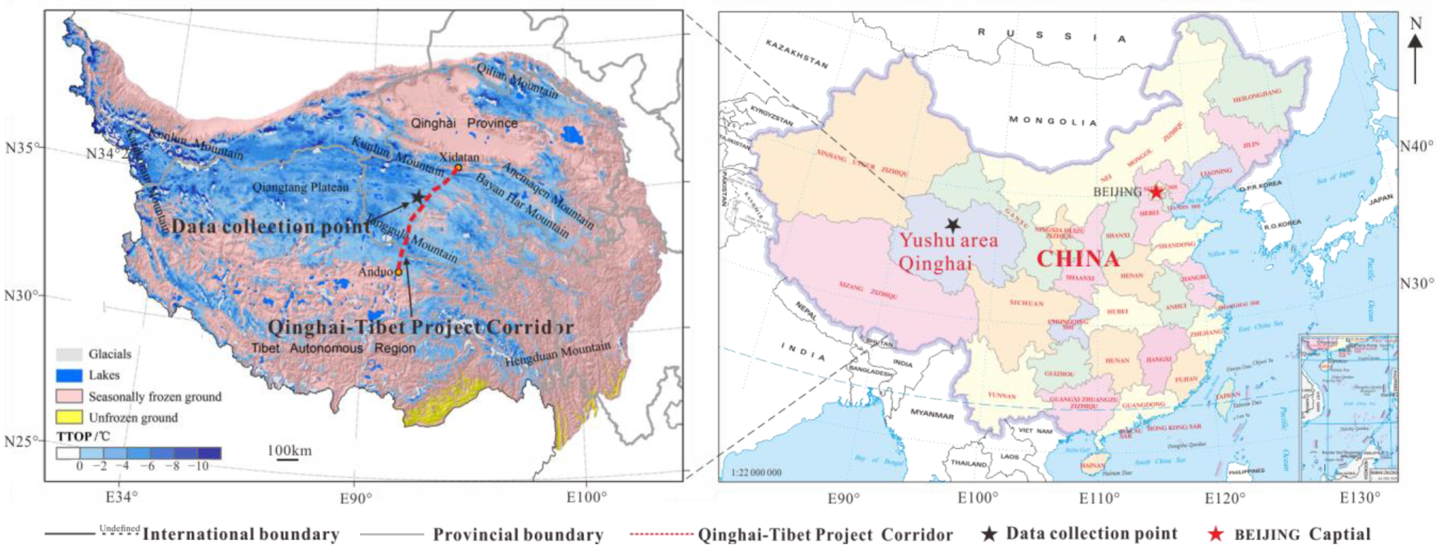
2.1. Study Area

The Qinghai–Tibet Plateau is in the western part of China, with an area of about 2.55 × 106 km². It is a representative area of high-altitude frozen soil in the world. The Qinghai–Tibet Project (including the Qinghai–Tibet highway, railway, high-voltage grid lines, oil pipeline, and ancillary settings of these projects) starts from Xining City, Qinghai Province to Lhasa City, Tibet Autonomous Region, forming a natural corridor of about 1120 km from north to south. The projects are built in the corridor called the “Qinghai–Tibet Project Corridor” [8].

Figure 1 shows the frozen ground distribution on the Qinghai–Tibet Plateau [24,25]. A large amount of seasonally frozen soil has developed in the pink area in the picture. The blue area shows the swamps and grasslands developed on seasonally frozen soils, with large water content and poor soil stability. The data set in Figure 1 is based on an improved medium-resolution imaging spectrometer, ground surface temperature, and other detection instruments to detect the freezing-thawing index and the top temperature model simulation of frozen soil. The data were verified and corrected through actual geological and soil surveys on the ground. The red dotted line represents Qinghai–Tibet Project Corridor. The black asterisk is the data collection point location of thaw-slumping. It is in the Beiluhe area, with an average elevation of 4500 m. Near the measuring point, much thaw-slumping developed. Therefore, the data of this measurement point has a certain degree of representativeness.

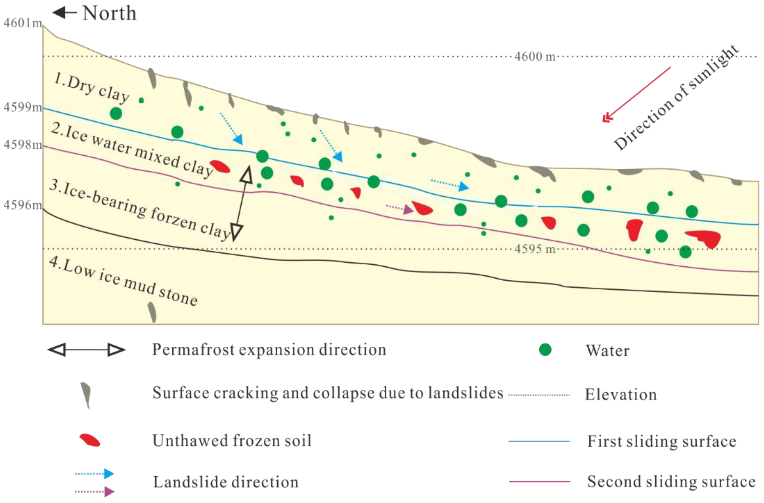
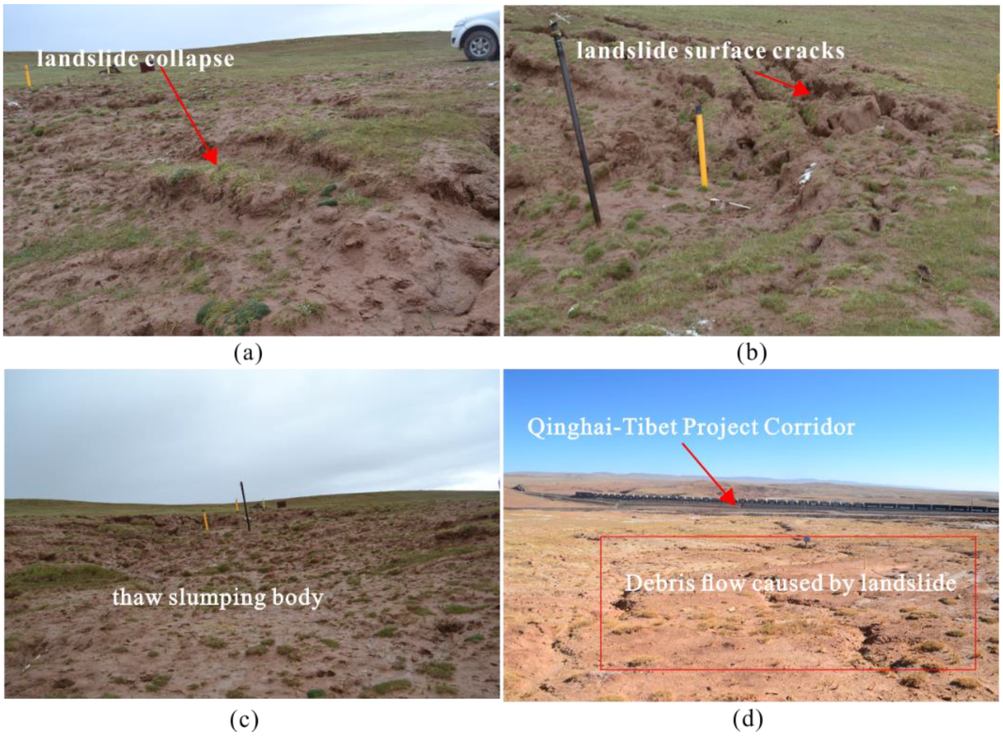
2.2. Overview of Thaw-Slumping Hazards

There are clay and fine sand substances with large water content in permafrost, and thick underground ice is generally distributed in the upper part of permafrost. The upper part of the ice layer is connected with the seasonal melting layer, and the lower part is connected with the permafrost in a layered distribution. Due to the influence of seasonal temperature and human factors, a series of freeze–thaw geological disasters, such as thermal thaw collapse and thaw mudflow, occur after the thawing of frozen soil distributed in slope areas. In the permafrost region of the Qinghai–Tibet Plateau, a slope with a gradient of more than 3 degrees may form a thermal melting collapse during the thermal melting process [18]. The surface frozen soil melts due to the temperature rise. Under the condition of high ice content, the sliding soil mass is a mixture of hard rock and soil blocks and liquid mud, which has low or no shear strength. Therefore, it is easy to generate a sliding surface roughly parallel to the slope surface [18,26,27,28].

Figure 2 is a schematic diagram of a frozen soil section with four layers of a layered structure. Among them, cracks and collapse appear on the surface of frozen soil due to the movement of frozen soil landslides and the change in water content. The underground water generated by the ablation seeps downward along the bedding plane and accumulates in the complete ablation layer and the ice-water mixed layer, resulting in maximum shear failure and landslide movement. With the increase of depth, there is unharmed frozen soil, ice-bearing frozen clay, and low-ice mudstone in turn. In addition, the change in water content in the soil caused by the thawing of frozen soil leads to the appearance of a landslide surface under dry clay and ice-water mixed clay layers. The difference in shear resistance and water content of different layers leads to the continuous collapse and soil cracks of the whole landslide mass and finally forms landslide hazards and ecological hazards.

Figure 3 is the site picture of the thaw-slumping hazard in this study. Figure 3a,b show the step-shaped collapse and surface soil cracks caused by landslides, respectively. Figure 3c shows the landslide body from the bottom to the top. Figure 3d shows the location relationship between the debris flow and Qinghai–Tibet Project Corridor. With the increase of hazards and the increase of landslide mass, the thaw-slumping has caused damage to the fragile ecological environment of the Qinghai–Tibet Plateau, and constantly threatened the engineering safety of the Qinghai–Tibet Highway.

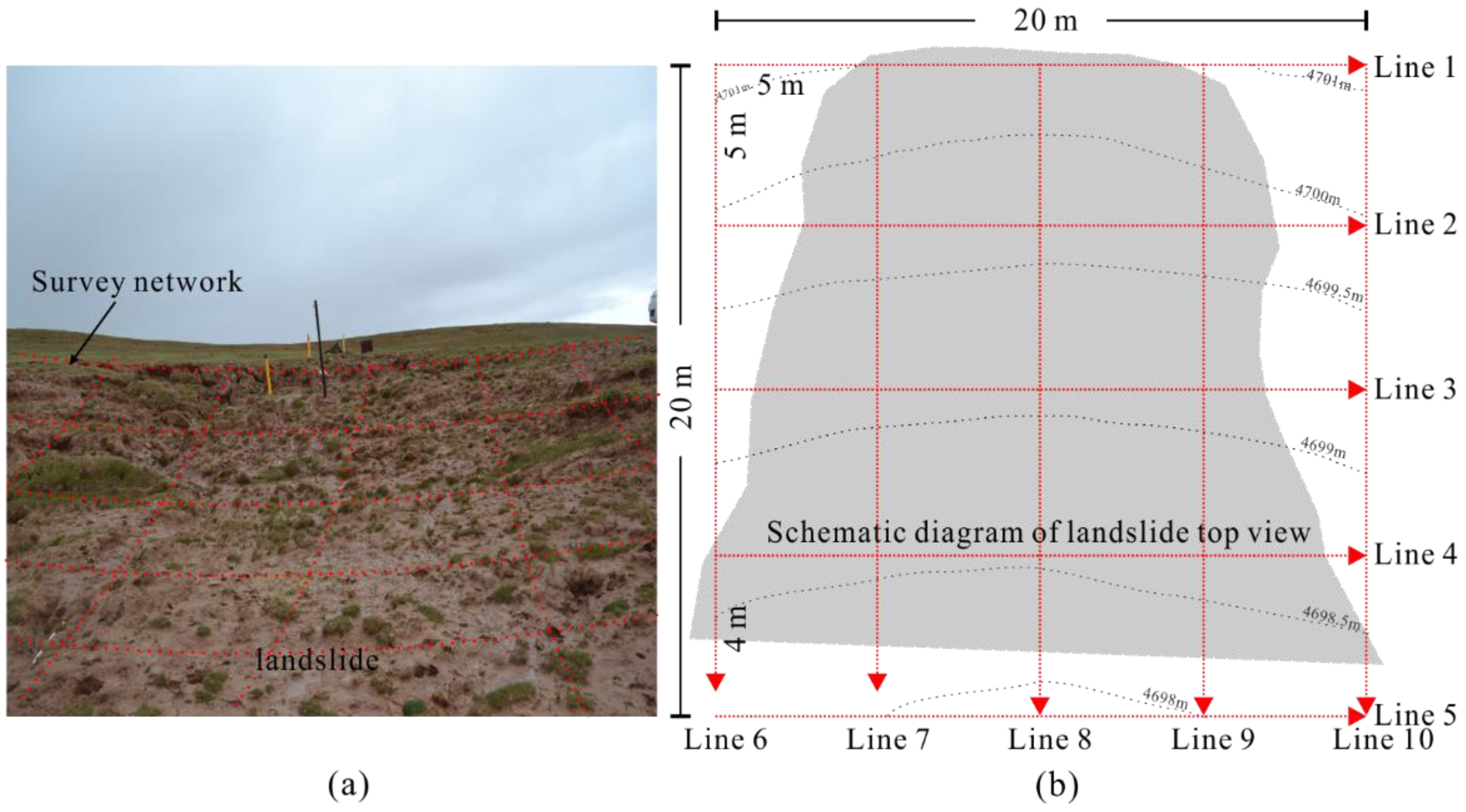
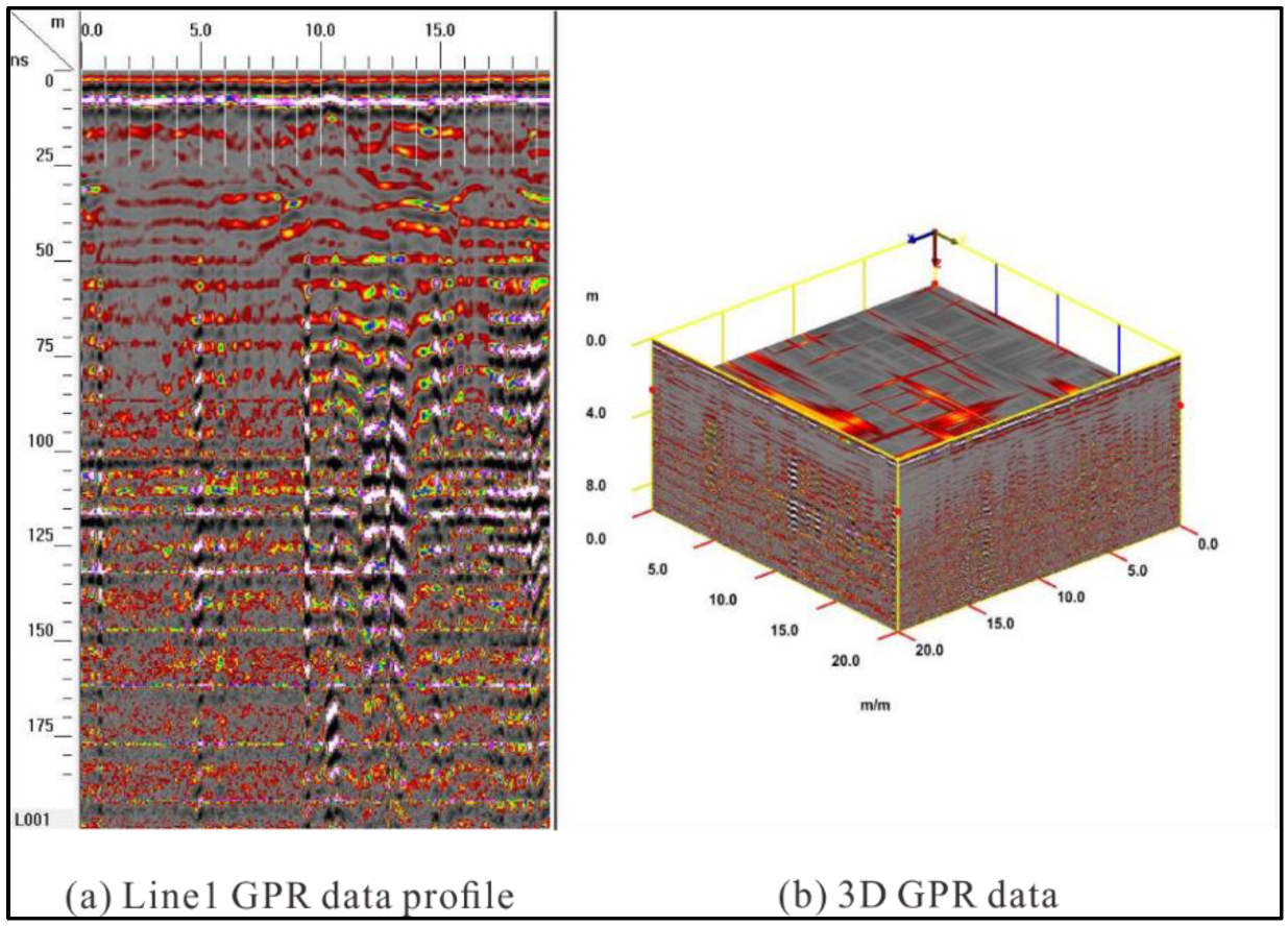
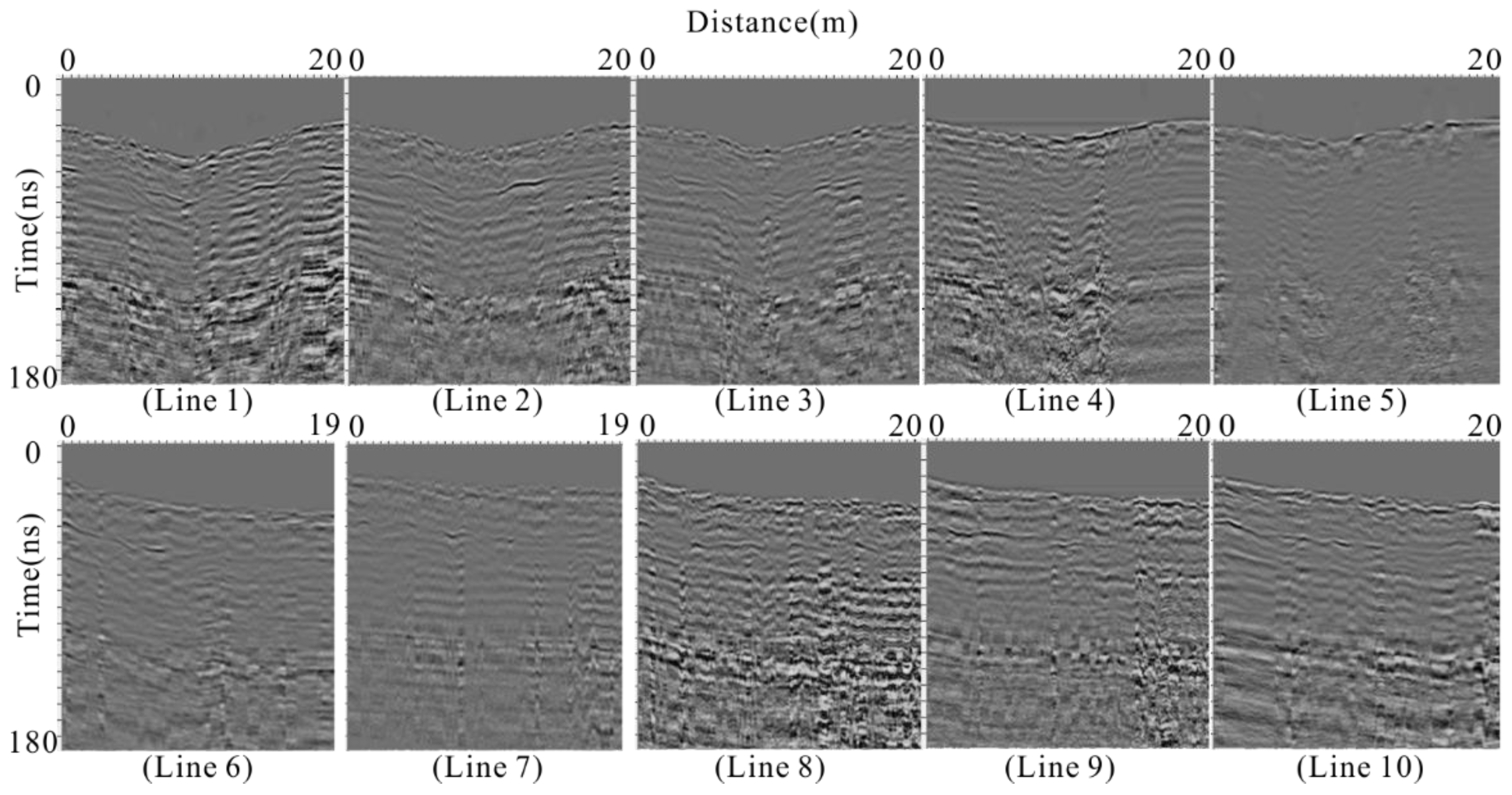
2.3. Test Site and Data Acquisition

To detect the landslide body more accurately, the test was carried out vertically and parallel to the direction of the landslide. In Figure 4a, the red dotted line indicates the actual measurement network layout. Under the combined action of gravity and ablation water, the middle position of the thaw-slumping body collapsed. The surface soil is cracked and uneven. Figure 4b shows the plan layout of the survey network, in which Line 6 and Line 7 are measured to 19 m due to topography. To form complete three-dimensional data, Line 6 and Line 7 continued to sample at 19 m to 20 m in situ.

Table 1. The specific parameters of measurement network layout.

Parameters	Values
Dimension	3
Line spacing	5 m
Number of lines	10
Line length	20 m

shows the specific parameters of the measurement network layout. Five survey lines are arranged in the longitudinal and transverse directions of the test site. Line spacing is 5 m.

To achieve the ideal measurement depth and resolution, this measurement uses an antenna with a center frequency of 200 MHz for data collection. The instrument used in this measurement is GSSI-SIR 4000, and the specific parameters of data acquisition are shown in

Table 2. The specific parameters of data acquisition by GSSI-SIR 4000.

Parameters	Values
antenna center frequency	200 MHz
scan/second	153
unit/mark	1 m
sample/scan	512
Time window	200 ns
Measurement mode	Survey wheel
Relative permittivity	10

. Due to the ablation of frozen ground on the ground, there is water in some areas, and the surface cracks and undulations are large. The use of shielded antennas has a stronger anti-interference ability against the external environment. Therefore, a shielded antenna was chosen this time. In data collection, to keep the antenna stable, the antenna and moving speed were reduced. We chose relatively flat ground for the layout of the collection line.

Figure 5 shows the original acquisition data and survey data presented by the GSSI processing software RADAN 7. Figure 5a shows the B-scan of Line 1, and Figure 5b shows the collected 3D data volume. The grayscale display of the raw data is shown in Supplementary Materials—Figure S1.

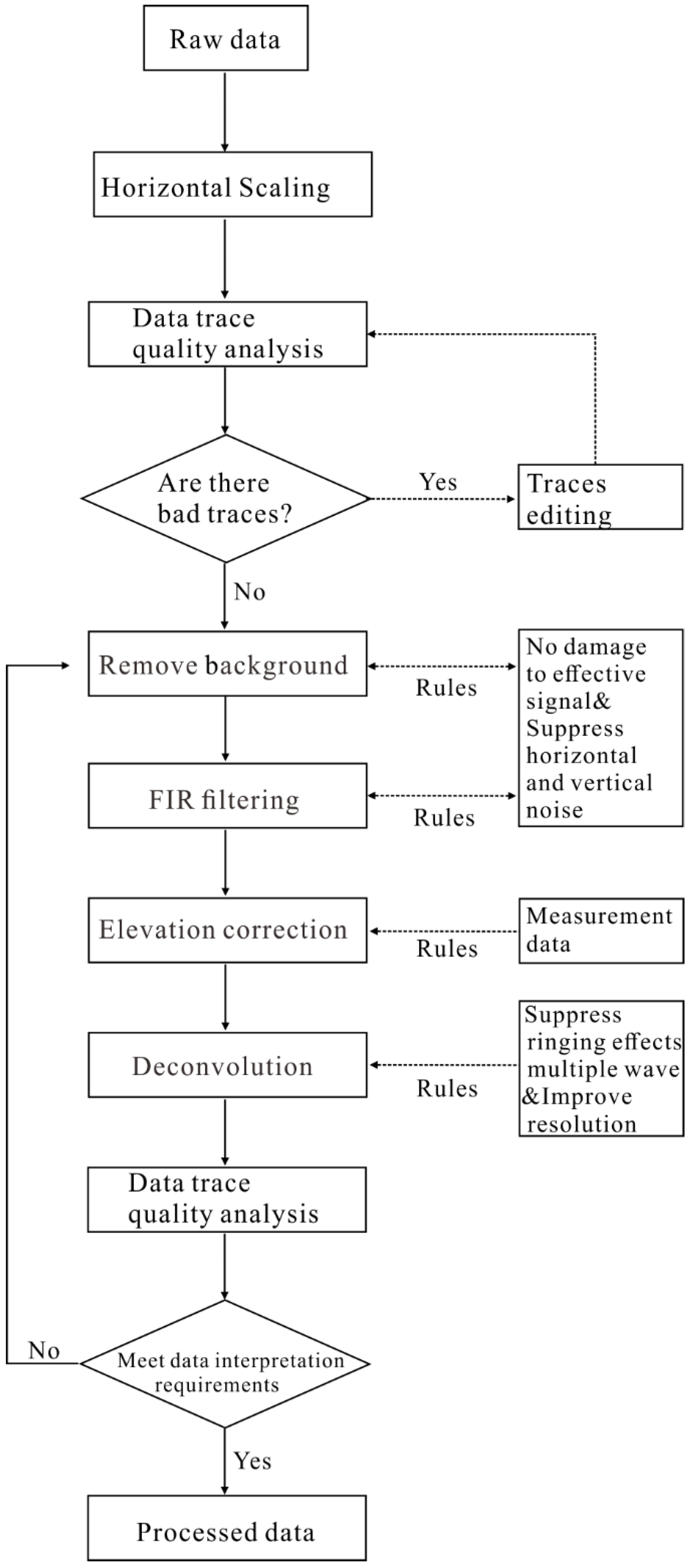
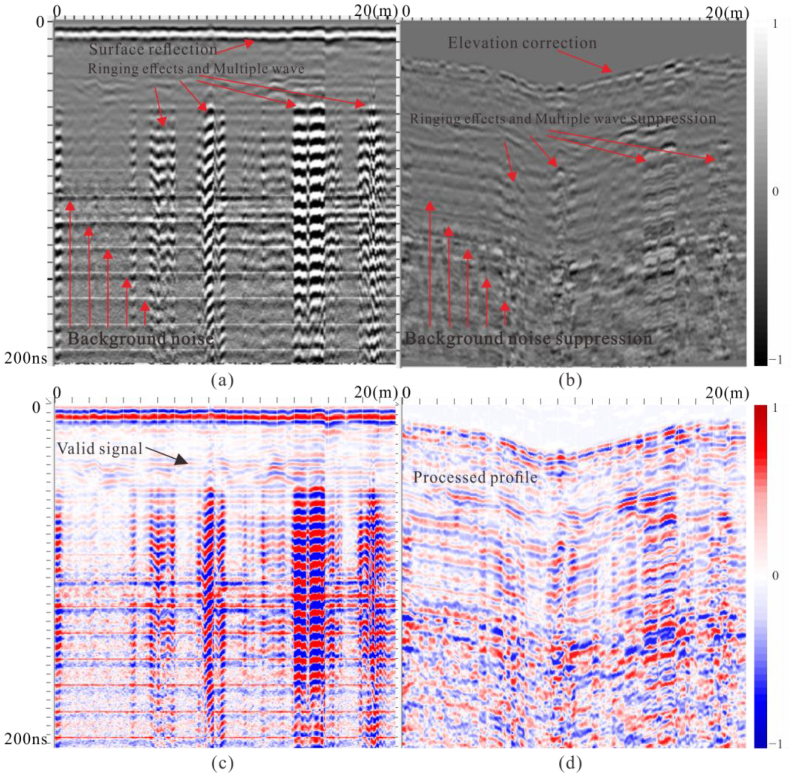
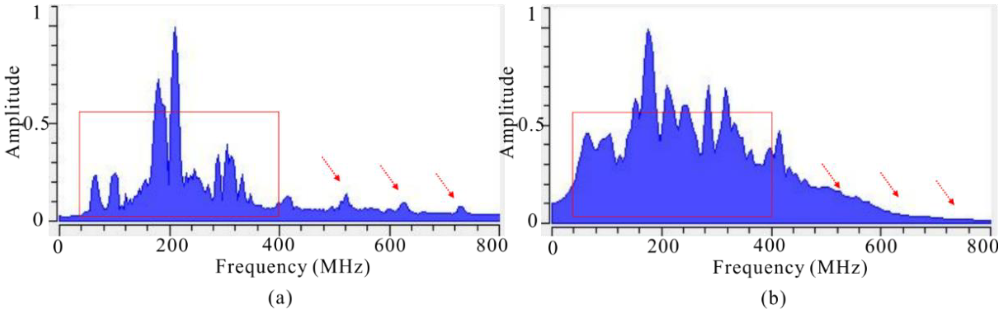
2.4. Data Processing

Methods such as horizontal scaling, traces editing, gain compensation, background noise suppression, FIR filter, IIR filtering, elevation correction, and deconvolution are used to process the data. Figure 6 is the data processing flow chart. Quality control runs through the whole data processing process.

Table 3. Processing process and basic parameters.

No.	Data Processing Method	Basic Parameters	Values
1	Horizontal scaling	Stretching of scans	3
2	Data trace quality analysis	Delete	Bad and invalid trace data
3	Gain compensation	AGC	3–6
4	Remove background	Full pass	Automatic calculation
5	FIR filtering	Bandpass	40 MHz~450 MHz
6	IIR filtering	Bandpass	30 MHz~500 MHz
7	Elevation correction	Boxcar	Measurement data
8	Deconvolution	Operator length	31
		Prediction lag	5
		Pre-whitening %	8
		Overall gain	2

records in detail the processing parameters used in each processing method.

Take the data of Line 1 as an example for analysis. Figure 7a shows the surface elevation error, background noise, and multiple noise and ringing effects in the original data in the grayscale image. The grayscale display offers the best contrast with the previous original image. To better highlight the noise suppression effect and the effective wave signal phase axis, a colored image display is adopted. Figure 7c shows the color display mode of the same amplitude signal. The effective signal is submerged in noise. Figure 7b shows the grayscale data after elevation correction, ringing effects, multiple suppression, and background noise removal. Figure 7d shows the color profile of the processed data. The effective signal has been significantly enhanced.

Figure 8 is a spectrum analysis diagram of Line 1 data before and after processing. After processing, the spectrum energy of 50–400 MHz has been significantly enhanced, and the spectrum burr caused by noise has also been suppressed (in the red box). In addition, ring effects and multiple interferences are effectively suppressed (red arrow). Data processing has achieved good results in effective frequency extension and improvement of signal-to-noise ratio.

2.5. Methods

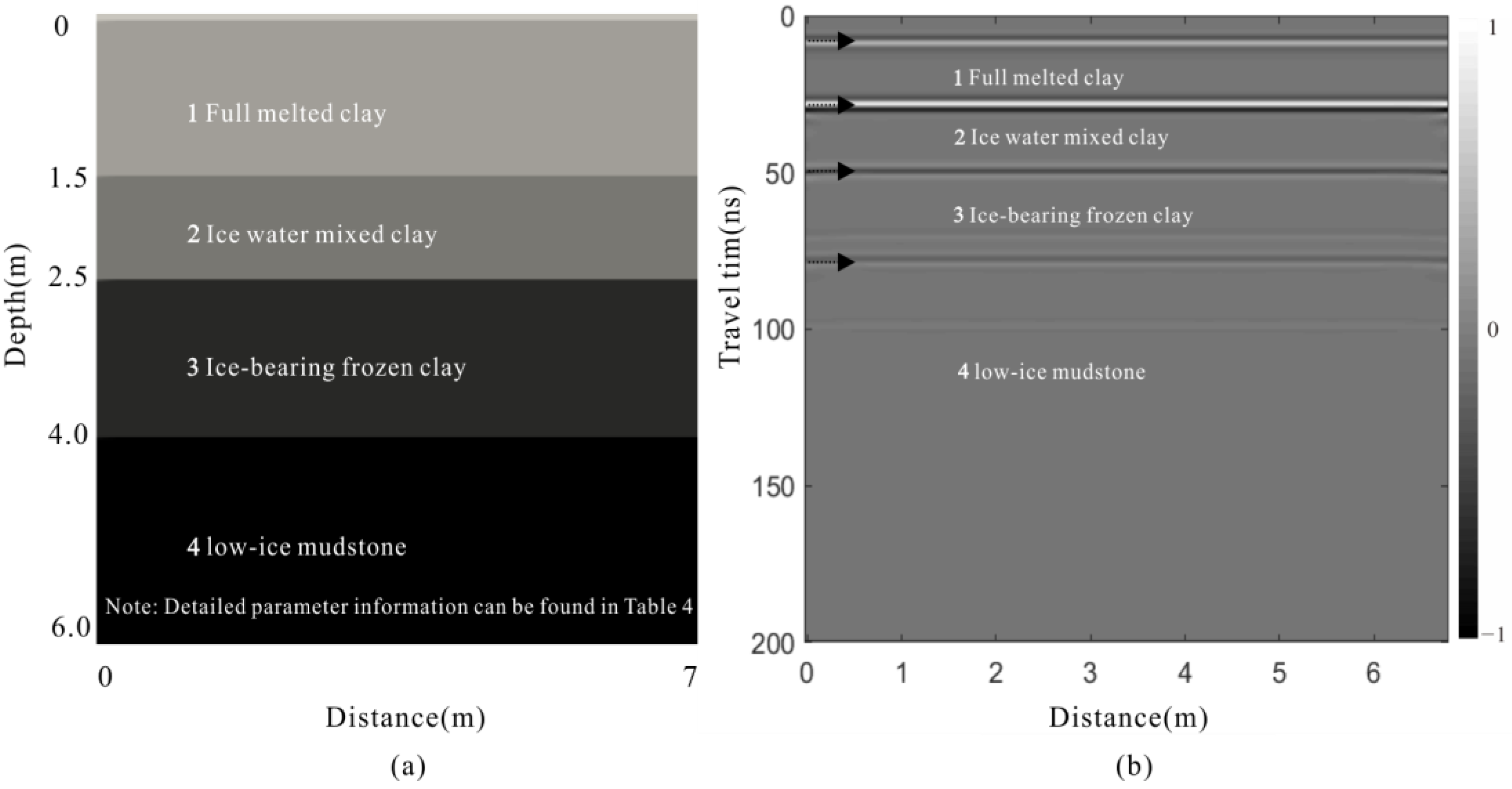
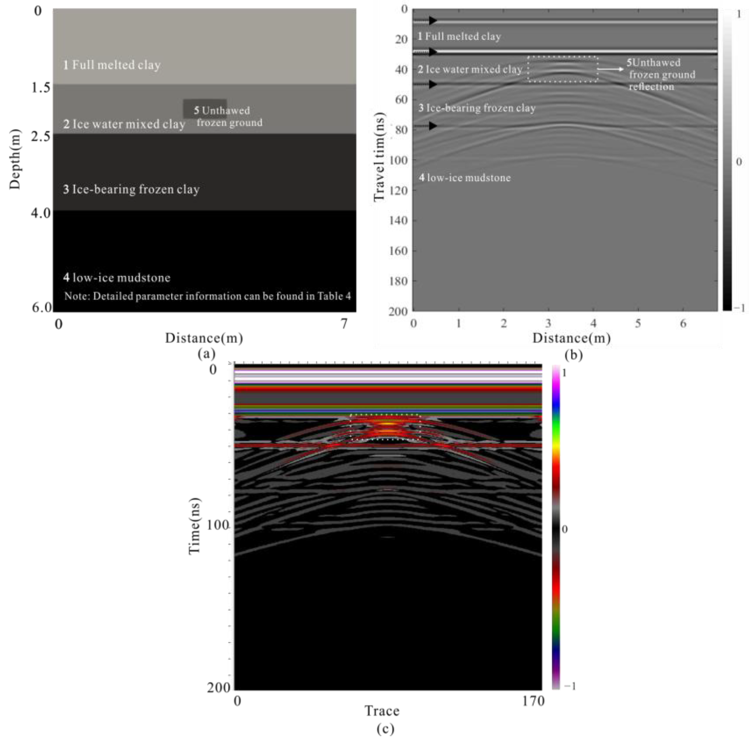
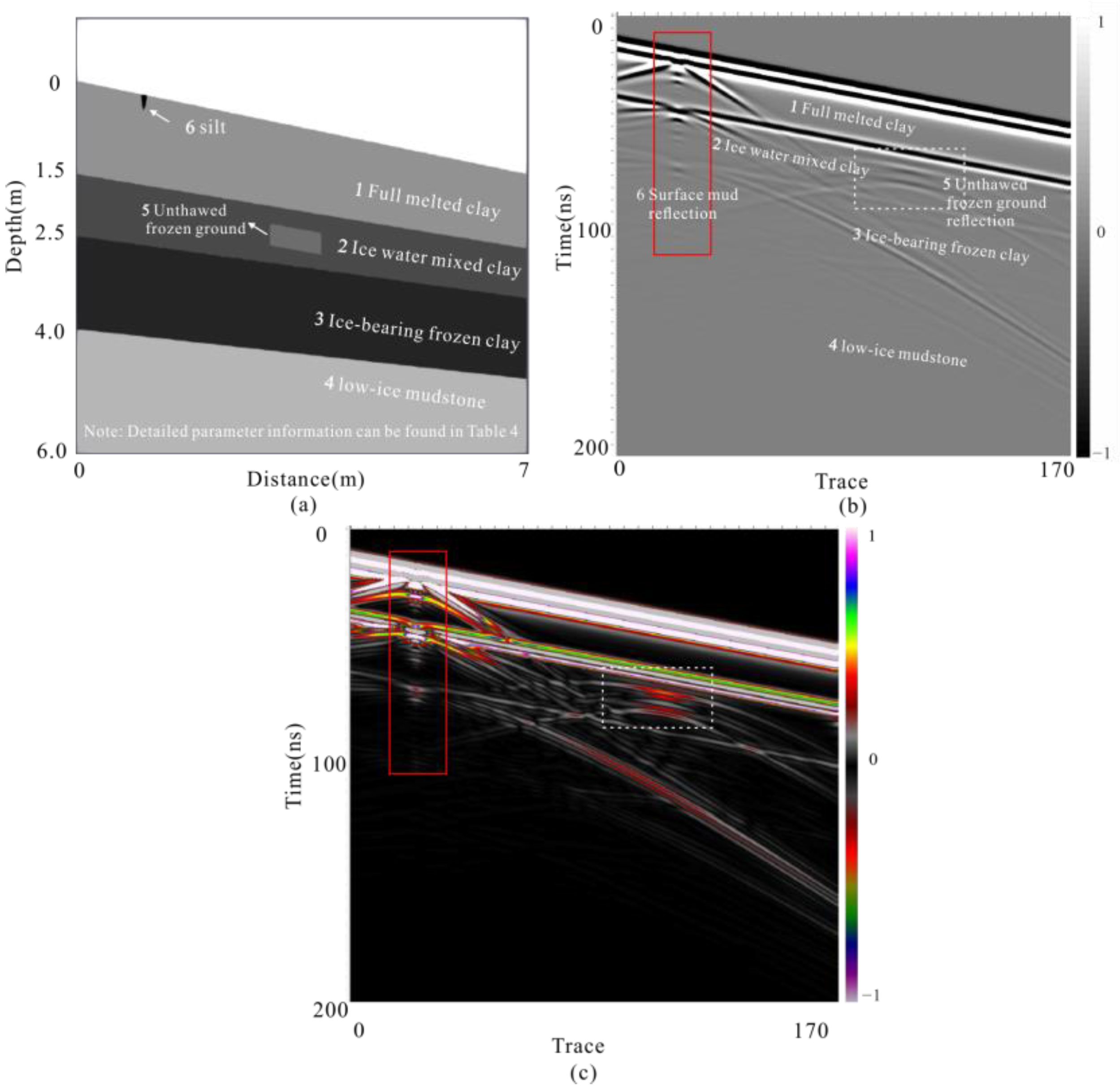
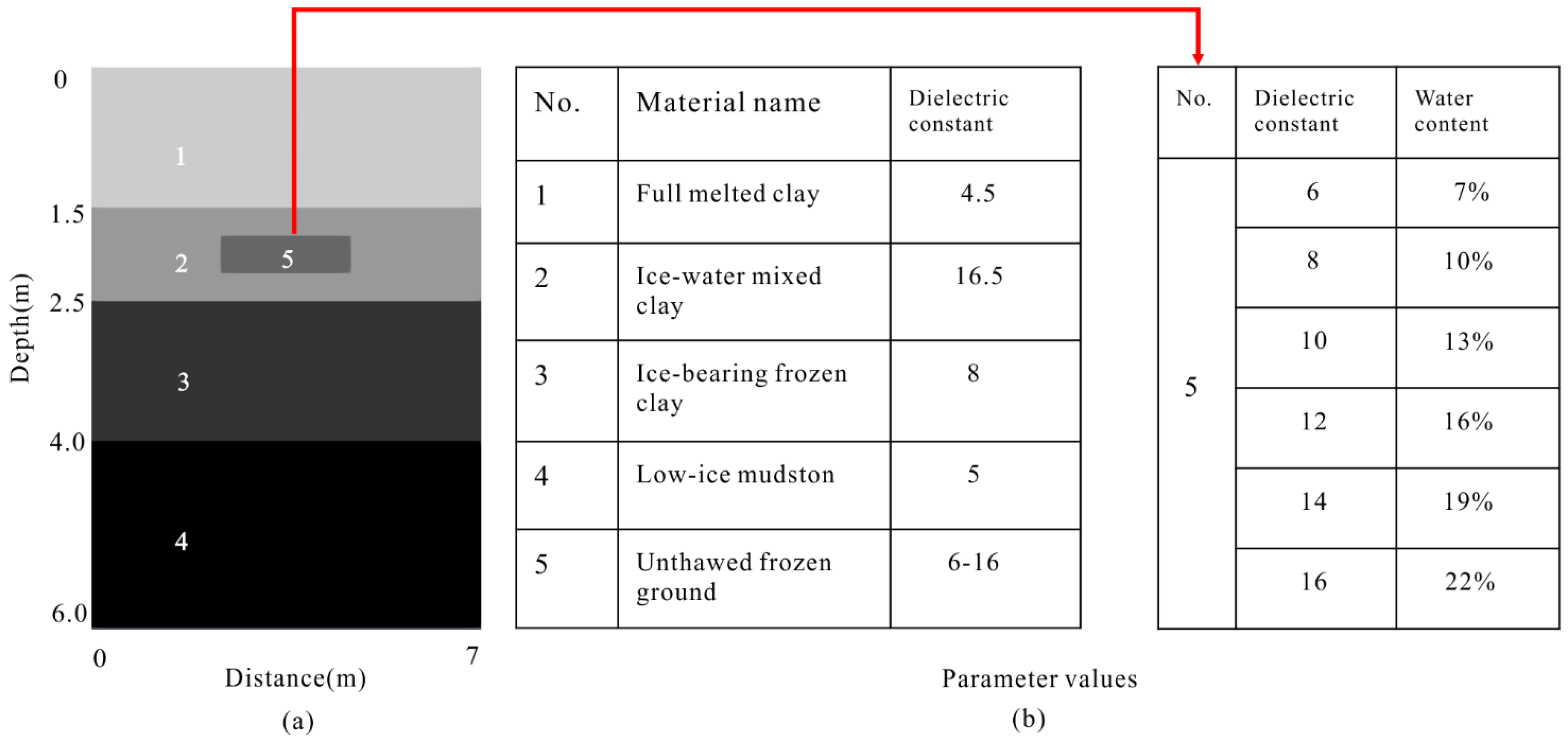
2.5.1. Simulation of Geometric Feature and Noise Reflection Characteristics

According to the previous research data, the frozen soil medium in the test site is divided into dry clay, ice-water mixed clay, ice-bearing frozen clay, and low-ice mudstone [18,22]. To study how to accurately divide the layers of the underground medium of thaw-slumping in GPR B-scan data, a frozen soil medium Model 1 with a 4-layer structure was established.

Table 4. Specific model parameters.

Media Serial Number	Media Type	Relative Permittivity ɛ	Conductivity Σ (S/m)	Depth (m)
1	Full melted clay	4.5	0.00027	0
2	Ice-water mixed clay	10	0.03	1.5
3	Ice-bearing frozen clay	8	0.001	2.5
4	low-ice mudstone	5	0.00015	4
5	Unthawed frozen ground	6	0.0003	2.4
6	silt	16	0.035	0

shows the specific information on the media parameters of all models.

The GPR signal is simulated by gprMax software. The gprMax is electromagnetic wave simulation software that is based on the Finite-Difference Time-Domain (FDTD) method. All electromagnetic phenomena, on a macroscopic scale, are described by the well-known Maxwell’s equations. In Maxwell’s equations, there are two curl equations, Faraday’s law of electromagnetic induction and Ampere’s law, and two divergence equations, Gauss’ law and Gauss’s law of magnetism. The finite-difference method in the time domain replaces Maxwell’s equations with finite-difference approximations, using two curl equations with a time variable to create a difference equation containing a space of discrete variables. A time-forward algorithm is constructed in turn to simulate the propagation of electromagnetic waves and solve the electromagnetic field parameters in the time domain [29,30,31,32,33]. Specific information such as grid parameters is shown in

Table 5. Simulation parameter setting information.

Domain (m)	dx_dy_dz (m)	Waveform	Antenna Transmitting and Receiving Distance (m)	Number of Acquisition Channels and Acquisition Time	Antenna Center Frequency
7 × 77	0.01	Ricker wavelet	0.04	170 trace and 200 ns	200 MHz

.

Figure 9a,b show the Model 1 and simulation data, respectively. The simulation is the amplitude grayscale display. The black arrow in Figure 9b shows the location of the layered interface in the model. Due to the change in electrical parameters, such as the dielectric constant, the wavelet produces a larger amplitude at the interface. Using the travel time rule, the simulated radar data horizon position was calculated, and the accuracy of the layering was verified.

To study the propagation characteristics of electromagnetic waves more accurately in different media, the differences in the division of the media based on their characteristics are used. Calculate the instantaneous amplitude attenuation of the radar data. Figure 10 shows the instantaneous amplitude decay curve of the simulated data. The brown, blue, purple, and green dashed lines, respectively, show the change in the attenuation value. In the simulated data, the continuity of the phase axis of the interface reflection is good, and no material distribution produces strong reflection amplitudes within the layer. Therefore, the strong reflection amplitude generated by interface reflection becomes a basis for dividing layers. However, in actual data, there may be uneven substances within the layer that generate strong reflection amplitudes, and their reflection intensity may exceed the interface reflection. Fortunately, the strong amplitude events generated by this non-uniform material in permafrost do not have continuity, making it difficult to track the interface, making it difficult to interfere with our use of the strong amplitude of continuity for layer division. Due to the differences in dielectric constant and absorption coefficient within different layers, the amplitude energy attenuation characteristics of electromagnetic waves within each layer may differ. The use of amplitude energy attenuation features can compensate for the shortcomings of only using strong amplitude to divide layers and minimize the error of using continuous strong amplitude for layer division. In the area between each dotted line, the attenuation changes are relatively consistent, indicating that there are media with the same electrical parameters. The time indicated by each dashed line is consistent with the interface time displayed by the grayscale image of the simulated data, which proves that the attenuation property can be used to divide the layer position of the medium. The actual medium particles are larger than the model, the reflected waveforms in the same layer are more abundant, and the attenuation attribute change trend calculated with actual data will be more obvious.

In the actual data analysis, it is found that there is much irregularly distributed unthawed frozen soil in the thawed frozen soil. The existence of ice-water mixed clay causes the anisotropy of the physical properties of the medium and increases the instability of frozen soil. Model 2 simulates this phenomenon. Table 4 shows the specific information of the Model 2 parameters. The specific simulation parameters are shown in Table 5. Model 2 uses the same simulation parameters as Model 1 for simulation. Figure 11a,b show the model and simulation data, respectively. The simulation is the amplitude grayscale display. The black arrow in Figure 11b shows the location of the layered interface in the model. The white box area is the reflection amplitude of the unthawed frozen soil. To compare with the actual data, Figure 11c highlights the amplitude reflection feature of unthawed frozen ground with a color mode in an ice-water mixed layer. Due to the presence of frozen soil, a strong amplitude reflection will be generated in the ablation medium. Under the influence of multiple reflections at the interface, the reflections from frozen soils have obvious characteristics of strong multi-phase axis reflections. The frozen soil in ice-water mixed clay will cause anisotropy of the medium, uneven distribution of water content, and instability of the formation. It is a key parameter in thaw-slumping hazards.

Due to the different dielectric constant and absorption and attenuation coefficient of Model 1 and Model 2, electromagnetic wave shows different propagation speed and energy attenuation trend in different media. Due to the difference in dielectric constant caused by the thawing of frozen soil, the electromagnetic wave has reflected amplitude on the interface of the medium with different degrees of thawing. In the interior of the medium, it shows different amplitude energy attenuation trends. This provides a basis for the division of different ablation layers using the amplitude event and amplitude energy attenuation trend.

To verify the characteristics of noise wave field at the radar interface when there is collapse or silt on the surface. Figure 12a establishes a new Model 3. The parameters of Model 3 are shown in Table 4. In Model 3, there is silt on the surface and unfrozen frozen soil in an ice-water mixed layer. Figure 12b shows the noise caused by obvious surface mud reflection (red box) and unmelted frozen soil reflection (white box) in grayscale mode. To compare with the actual data, Figure 12c shows these two wave field characteristics in color mode. The simulation results are basically the same as the actual data.

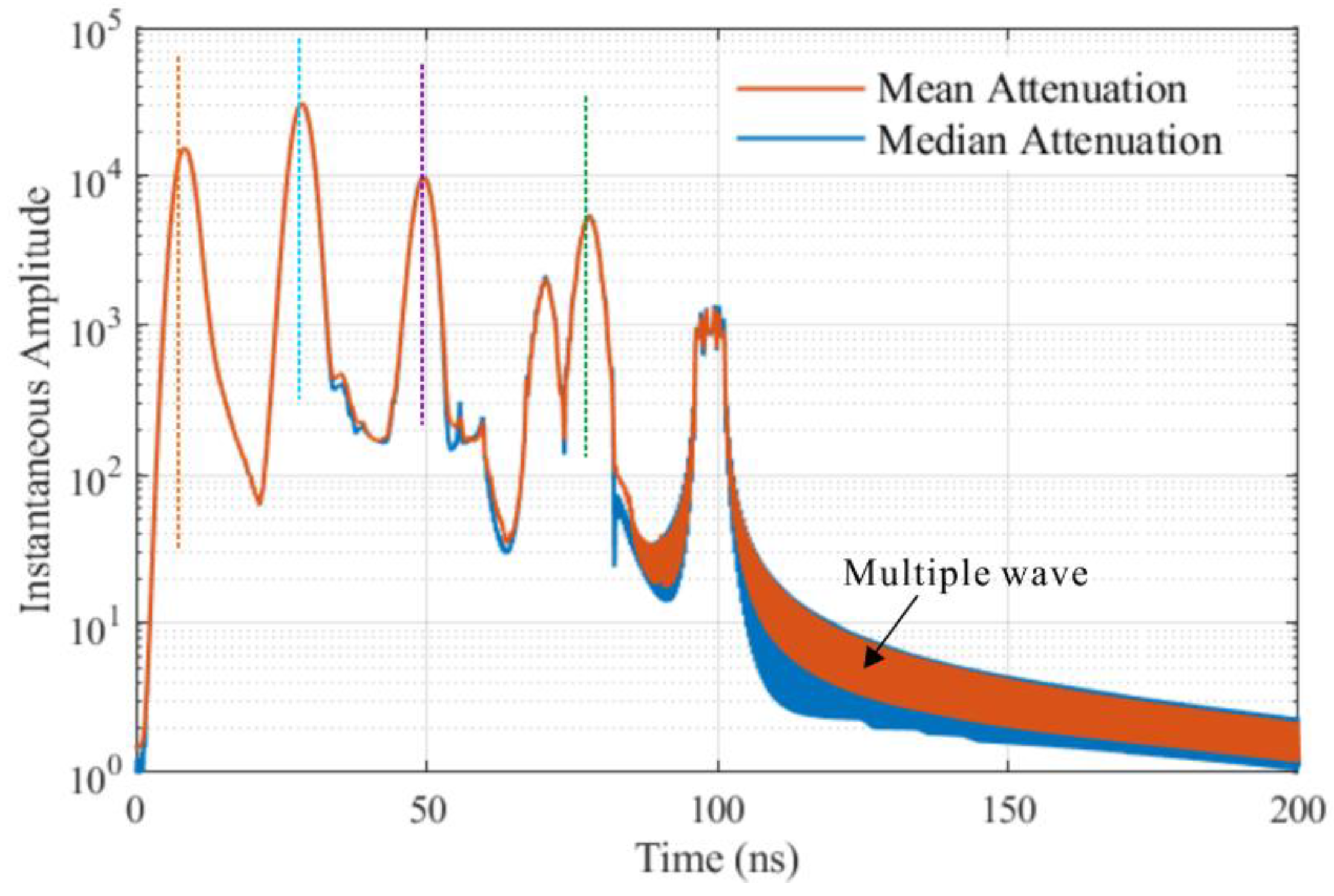
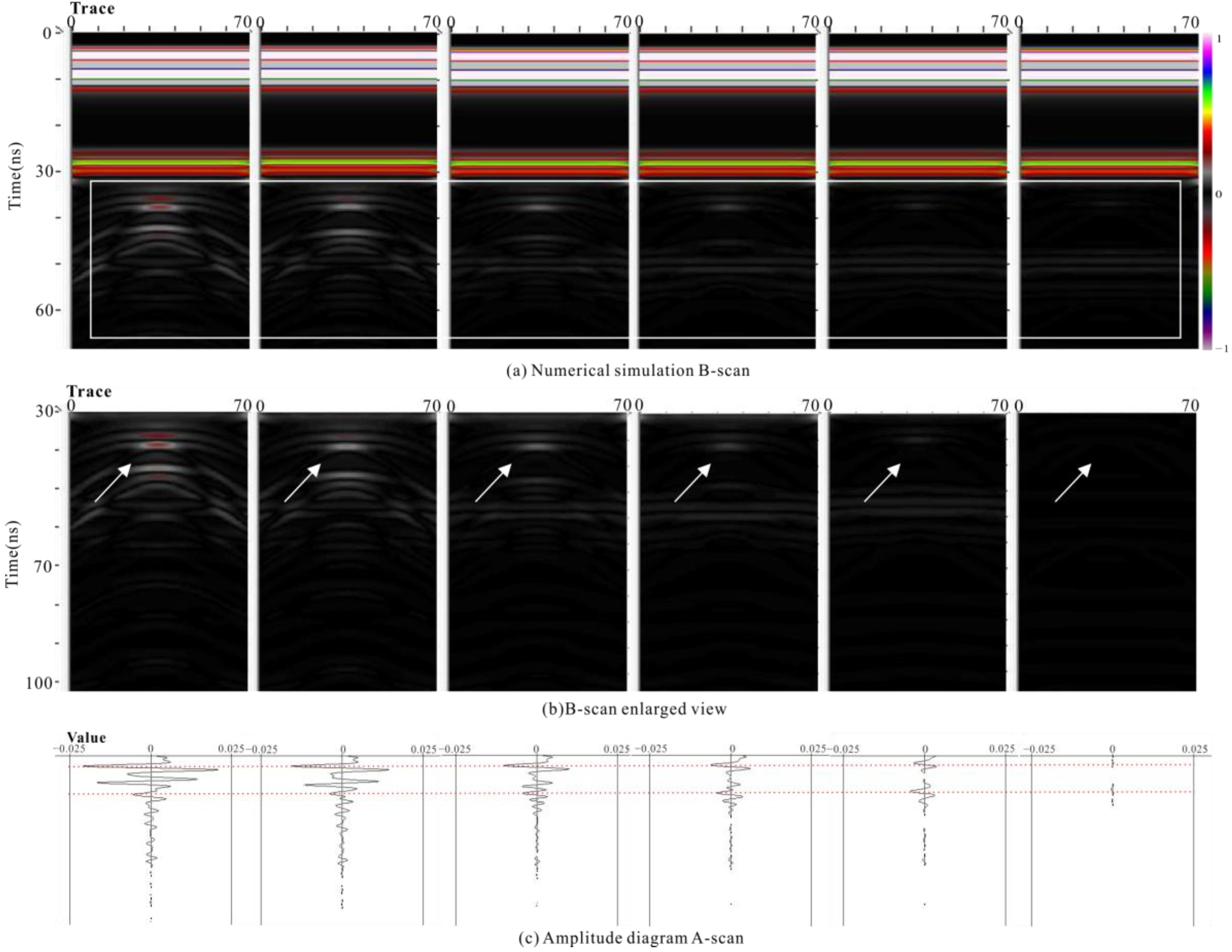
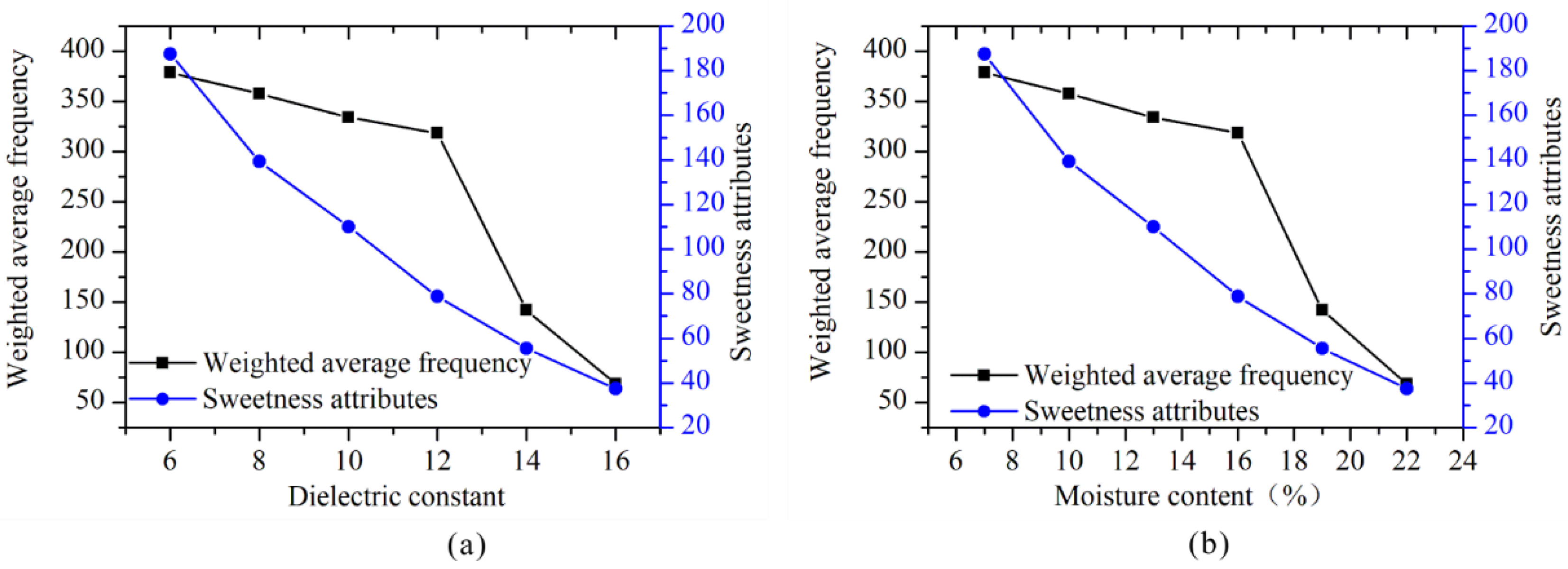
2.5.2. Simulation of Amplitude Characteristics of Water Content Change

The prediction of absolute or relative water content in frozen soil is one of the key tasks of frozen soil radar detection. The difference in water content in frozen soil leads to the change in the dielectric constant of the medium, which will be reflected in the radar amplitude. To verify the correlation between frozen soil water content and radar amplitude data, Model 4 is constructed. Based on the analysis and accumulation of data from local soil samples, the basic correspondence between relative dielectric constant and water content has been determined. A frozen soil model with different water content is established in Figure 13, where the unthawed frozen ground (No. 5) is in ice-water mixed clay (No. 2). The ice-water mixed clay represented by No. 5 contains six different water contents, which are 7%, 10%, 13%, 16%, 19%, and 22%, respectively.

Model 4 is simulated six times with the parameters in Table 4. Figure 14 shows the simulation results of different water content models. From left to right, the simulation results of water content models are 7%, 10%, 13%, 16%, 19%, and 22%, respectively. Figure 14a shows the simulated raw B-scan data. Figure 14b is an enlarged display of ice-water mixed clay (No. 2) radar reflection amplitude in the white box of the original B-scan data. Compared to Figure 14a, Figure 14b selects data from the time interval of 30–100 ns to avoid interference from direct ground waves and strong interface reflections on data visual recognition. In addition, Figure 14c is the center channel reflection amplitude A-scan data of Figure 14b data. Figure 14c is the maximum amplitude diagram of reflection corresponding to the unthawed frozen ground (No. 5) with different water content. The melting water produced by frozen soil is mainly concentrated in the ice-water mixed clay layer. The prediction of the water content and distribution position of frozen soil in this layer can better serve the evaluation and prevention of thaw-slumping hazards. With the increase in water content, the dielectric constant of the partially thawed frozen soil increases continuously. When the dielectric constant increases to the same as the background medium (ice-water mixed clay), its corresponding amplitude gradually decreases (Figure 14c). Therefore, the amplitude value can be used to determine the relative water content in frozen soil. Parameter values extracted from Figure 14 are shown in

Table 6. Parameter values extraction from Figure 14.

Parameter	Numerical Value
Maximum amplitude value	0.02	0.014	0.009	0.0059	0.0024	0.00028
Dielectric constant	6	8	10	12	14	16
Water content	7%	10%	13%	16%	19%	22%

.

2.5.3. Calculation Method of Relative Water Content

The prediction of the water content of the ablation layer is an important part of the characterization and evaluation of the thawing slumping layer. Although the borehole coring measurement technology can obtain the absolute value of water content with high accuracy, its efficiency is low and only the value of sampling points can be obtained, which will also cause damage to the thaw-slumping. Due to the abnormal characteristics of water in GPR signals, it is possible to measure water content by GPR [28,34,35,36,37]. The Topp formula can be expressed as:

$$\theta =-5.3\times {10}^{-2}+2.92\times {10}^{-2}\mathsf{\epsilon }-5.5\times {10}^{-4}{\mathsf{\epsilon }}^2+4.3\times {10}^{-6}{\mathsf{\epsilon }}^3$$

(1)

where ɛ is the dielectric constant of the medium. To obtain the dielectric constant of the medium from the GPR signal, it is necessary to calculate the electromagnetic wave velocity in the medium. In the calculation of velocity, the GPR observation system needs to use the common middle point (CMP) gathers. Due to landslide slope, surface collapse, and antenna power limitation, CMP mode is not suitable for data acquisition of thaw-slumping on the plateau. In addition, the velocity obtained by the CMP observation method is the layer velocity of the medium, and it cannot obtain the lateral velocity value of the frozen soil layer in a short distance, which has a low effect on predicting the change in the dielectric constant and water content in the thaw-slumping. To make full use of GPR data to calculate medium water content, the Topp formula has been improved a lot. These improvements are carried out around the velocity and dielectric constant, and replacing the dielectric constant value with the ground-penetrating radar attribute is an important improvement research direction [38,39,40,41,42]. Ground-penetrating radar attributes refer to seismic attribute theory. The geometric, dynamic, and statistical characteristics in its waveform records reflect the structure and physical properties of underground media. The amplitude, frequency, and waveform of the signal are related to the shape, dielectric constant, attenuation coefficient, and other physical parameters of the underground medium [43,44,45,46]. Through the calculation of the GPR signal attributes simulated by Model 4, the attribute information related to water content can be obtained, which can provide a reference for the improvement of the Topp formula. To reduce the error and multiplicity caused by a single attribute,

Table 7. Statistical table of correlation coefficient between GPR attribute and water content.

No.	Radar Attribute	R	No.	Radar Attribute	R
1	waveform difference	0.42	10	relative impedance	0.71
2	instantaneous amplitude	0.68	11	average weighted frequency	0.84
3	instantaneous frequency	0.52	12	thin-bed indicator	0.25
4	instantaneous phase	0.35	13	sweetness	0.82
5	instantaneous bandwidth	0.24	14	phase rotation	0.15
6	instantaneous dominant frequency	0.41	15	response frequency	0.22
7	instantaneous Q	0.48	16	instantaneous acceleration	0.10
8	response phase	0.28	17	cosine of instantaneous phase	0.18
9	amplitude	0.86	18	apparent polarity	0.21

lists the correlation coefficients between 18 GPR signal attributes and water content.

In Table 7, the correlation coefficients of the amplitude attribute, average weighted frequency attribute, and sweetness attribute are high. The amplitude has a great correlation with the dielectric constant of the medium. It has a direct response to changes in the dielectric properties, which can be used as a calculation attribute to replace the dielectric constant in the Topp formula to calculate the relative water content of the medium.

Figure 15a,b show the relationship between the average weighted frequency and sweetness, dielectric constant, and water content. These two attributes have a certain linear relationship with the dielectric constant and water content. Due to some noise interference on the GPR signal, the instantaneous frequency curve has too many ups and downs. To prevent this phenomenon, the weighted average frequency is proposed and applied to highlight the main frequency characteristics of the wave [47,48]. Early studies in this area have shown that the weighted average frequency attribute can better reflect the temperature change trend of the frozen soil in the ablation zone, not the absolute value of temperature [23]. The numerical variation in the weighted average frequency attribute shows a good correlation with the variation in ground temperature. In addition, because the temperature has a direct correlation with the thawing of frozen soil, and has a good correlation with the dielectric constant of the thermal-thawing landslide medium, this attribute is put into the formula to replace the dielectric constant calculation. Weighted average frequency $\varpi (t)$ is defined as follows [46]:

$$\varpi \left(t\right)=\frac{{{\displaystyle \sum }}_{n=0}^{N=+\infty }{a}_n^2\left(t\right){\phi }_n^{’}\left(t\right)}{{{\displaystyle \sum }}_{n=0}^{N=+\infty }{a}_n^2\left(t\right)}$$

(2)

where $a_n\left(t\right)$ is a constant parameter. ${\phi }_n^{’}\left(t\right)$ is the derivative phase of the signal. There are many scattered water, collapse, crack, and surface undulations in the thaw-slumping area, which causes certain noise and short-wavelength problems in the radar data. These noises and short wavelengths will bring difficulties to the frequency analysis of the data. The weighted average frequency can overcome the influence of these two factors [27,46].

It is difficult to determine the size of the sweetness attribute value from the perspective of geophysics, which is only a relative concept. Previous research shows that the sweetness attribute can well classify the lithologic types of sandstone and mudstone [49,50]. Especially in the area with obvious wave impedance differences. This attribute has a better effect on lithologic classification. Mathematically, the sweetness attribute is the ratio of reflection intensity to the square root of instantaneous frequency [51]:

$$S=\frac{R}{\sqrt{f_{inst}}}$$

(3)

where R is reflection intensity. $f_{inst}$ is instantaneous frequency. S is a sweetness attribute. The unmelted medium of thaw-slumping, especially in ice-water mixed clay, has a large reflection intensity. The difference in water content also leads to the difference in frequency in the GPR reflection signal of the medium. The soil in the permafrost regions of the Qinghai–Tibet Plateau contains sand. Sand and clay have different storage capacities for water, and clay is easier to store water. In addition, due to the presence of unmelted frozen soil, its dielectric constant is closer to sand [18,22]. Combined with the linear relationship between water content and sweetness attribute, these factors show that the sweetness attribute can be used to effectively distinguish the media with different water content in thaw-slumping media. To sum up, first of all, there is a good linear correlation between the three attributes and the water content and dielectric constant of frozen soil; Second, the amplitude attribute can reflect the change in the dielectric constant of thawed frozen soil, the weighted average attribute can reflect the temperature change trend of the thawing medium, and the sweetness attribute can divide the medium lithology with different water content in the thawing medium; Finally, to reduce the data error caused by a single attribute, the three attributes are averaged to obtain a relative water content estimation factor:

$$\delta =\frac{A+\varpi +S}{3}$$

(4)

where amplitude attribute A, weighted average frequency attribute $\varpi$, and sweetness attribute S are the normalized values parameters. To overcome the disadvantage that it is difficult to obtain the underground dielectric constant that varies in both vertical and horizontal directions from GPR data, and reduce the error caused by the single dielectric constant calculation, the dielectric constant in Formula (1) is replaced by the relative water content estimation factor, and a new relative water content calculation formula based on the GPR signal attribute is obtained:

$${\theta }^r=-5.3\times {10}^{-2}+2.92\times {10}^{-2}\delta -5.5\times {10}^{-4}{\delta }^2+4.3\times {10}^{-6}{\delta }^3$$

(5)

where ${\theta }^r$ is relative water content. δ is the relative water content estimation factor. The methods mentioned above will be applied to the processing and analysis of the actual data below.

3. Results

After the ground-penetrating radar data are processed, the signal-to-noise ratio is improved, the effective signal is enhanced, and the influence of noise on data analysis and calculation is reduced. Due to the difference in ablation degree, the underground medium of thaw-slumping has different water content and dielectric constant. Both the model’s analysis and the early research have proved the stratification phenomenon of frozen soil after thawing, and the GPR signal has the same phase axis of amplitude at the frozen soil stratification [18,22,42]. In addition, due to the difference between the dielectric constant and absorption attenuation coefficient, the GPR signal’s Amplitude energy attenuation trend is also significantly different in different permafrost thawing layers. Combined with the actual frozen soil excavation data, it can well divide the horizon and demarcate the depth of the underground medium of thaw-slumping. Based on this stratigraphic framework, research the attributes of electromagnetic wave signals that can reflect changes in soil physical properties, ground temperature, and dielectric constant. Calculate the relative water content of the soil and provide the key elements of landslide development characteristics for disaster evaluation.

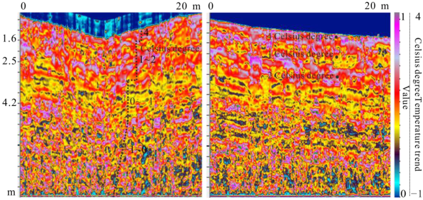
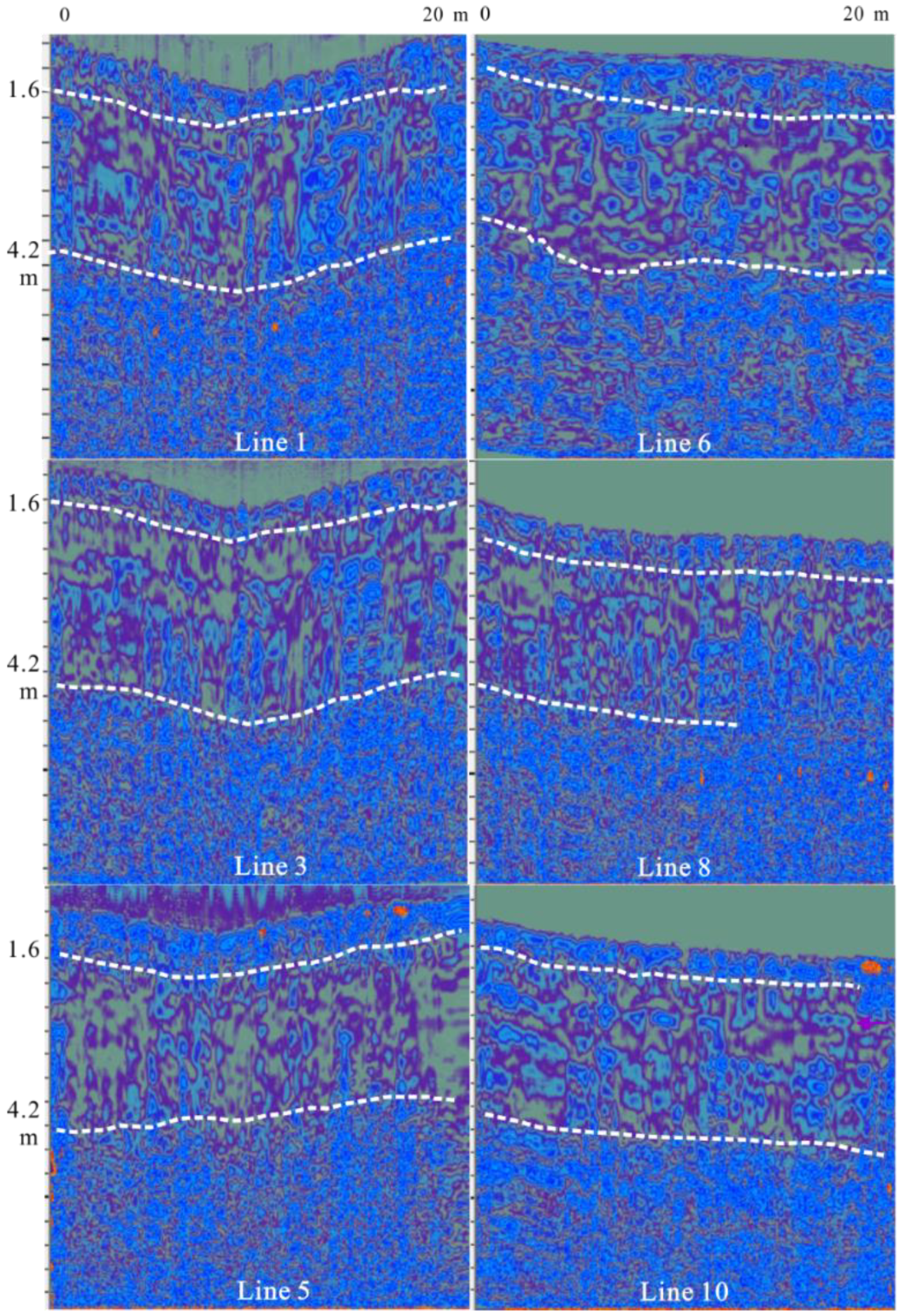
3.1. Stratification of Thaw-Slumping

The internal landslide surface of thaw-slumping often occurs on the contact surface of completely ablated and unthawed frozen soil. The layer division of the underground medium is the basis for the study of thaw-slumping. The originally collected radar data requires complete signal processing. The same processing method is used for all data to carry out elevation correction, multiple suppression, noise suppression, and migration imaging. Figure 16 shows the GPR grayscale profile from Line 1 to Line 10. It can be seen from the grayscale image that the event axis of the ground reflection has jumped. This is due to the development of surface cracks and unevenness (Figure 3 and Figure 17). Although the amplitude events on B-scan can be used to divide horizons, the tracking is interrupted due to the discontinuity of some regional events in the B-scan. In this case, the amplitude energy attenuation trend can be used for supplementary analysis to determine the specific depth of the horizon.

Due to the presence of unmelted frozen soil, there is a strong reflection amplitude in the ice-water mixed layer. However, this strong reflection amplitude event does not show good continuity and traceability, and cannot be used as a basis for layer division. The variation in amplitude energy attention trend can supplement the deficiency of using only strong amplitude for layer division. The amplitude energy attenuation calculation is performed on the processed data. The brown, blue, purple, and green dashed lines in Figure 18, respectively, represent the turning points of the trend of amplitude energy attenuation.

The change in attenuation trend is directly related to electromagnetic wave parameters such as the dielectric constant of the soil medium. Because the amplitude event can divide the strata, the amplitude energy attention is a supplement and evidence to the division result of the amplitude event. In Figure 18, it can be seen that the slope of the amplitude energy absorption trend in different layers is different, and some show significant positive and negative differences. Changes in this value reflect changes in soil water content, ice content, and soil composition. Combined with the actual soil excavation data, it is analyzed that the brown, blue, purple, and green dashed lines represent the boundary of the surface layer boundary, the fully melted layer boundary, the ice-water mixed layer boundary, and the ice-bearing boundary, respectively. Due to the large amount of water at the bottom of the thaw-slumping body and the accumulation of more melted soil, the depth of the ice-water mixed layer at the bottom of the landslide body measured by Line 4 and Line 5 continues to deepen and approach the boundary of the ice-bearing layer.

After completing the noise suppression of the data, we found that there are still strong reflection echoes in the complete ablation zone in the data. These strong reflections come from the unthawed frozen soil, and its dielectric constant is quite different from the physical properties of the surrounding medium.

Figure 19 shows the amplitude profiles of Line 1, Line 3, and Line 5. Among them, (a), (c), (e) and (b), (d), (f) correspond to the data, respectively. The (a), (c), and (e), respectively, show the amplitude B-scans of Line 1, Line 3, and Line 5 without elevation correction, which are used to supplement the analysis of soil structure changes and layer division. The white dashed line shows the layered boundary of the soil. The colored arrow on the right side of the white dotted line represents the layered boundary in Figure 18, and its color represents the same meaning as Figure 10. Each white dashed line corresponds to a border represented by a color. It can be seen from the amplitude profile that the layer tracked by the amplitude event axis is completely consistent with the layer divided in Figure 18. The white arrows in Figure 19 indicate strong reflections in the overall weak reflection background of the ice-water mixed layer. These strong reflections are related to the ice content in the soil medium. Frozen soil that has not been melted shows strong amplitude reflections in electromagnetic wave imaging. In addition, cracks appeared in the soil on the surface of the thaw-slumping due to melting and collapse, and water flowed to the deep part of the soil and the bottom of the thaw-slumping. Strong reflections also appeared in the soil above the boundary of the completely melted layer indicated by the blue arrow. These reflections are related to the undulating and dry cracking characteristics of the topsoil.

Figure 20 shows the amplitude B-scan of line 6, Line 8, and Line 10. The layer divided by the white dashed line in the figure is consistent with the layer represented by the colored arrows. Due to the accumulation of water at the bottom of the thaw-slumping and the melting and accumulation of soil, the layer divided by the white dashed line becomes deeper on the right side of each section (the bottom of the thaw-slumping), especially the boundary of the ice-water mixed layer. Survey Line 8 is at the position of the central axis of the thaw-slumping, and the Line 8 profile in Figure 20 shows that the boundary of the ice-water mixed layer at the bottom of the landslide has become blurred (white box). Combined with the actual soil excavation data, we layered the soil of the thaw-slumping. The thaw-slumping can be divided into a fully melted layer, an ice-water mixed layer, an ice-bearing layer, and a low-ice mudstone layer.

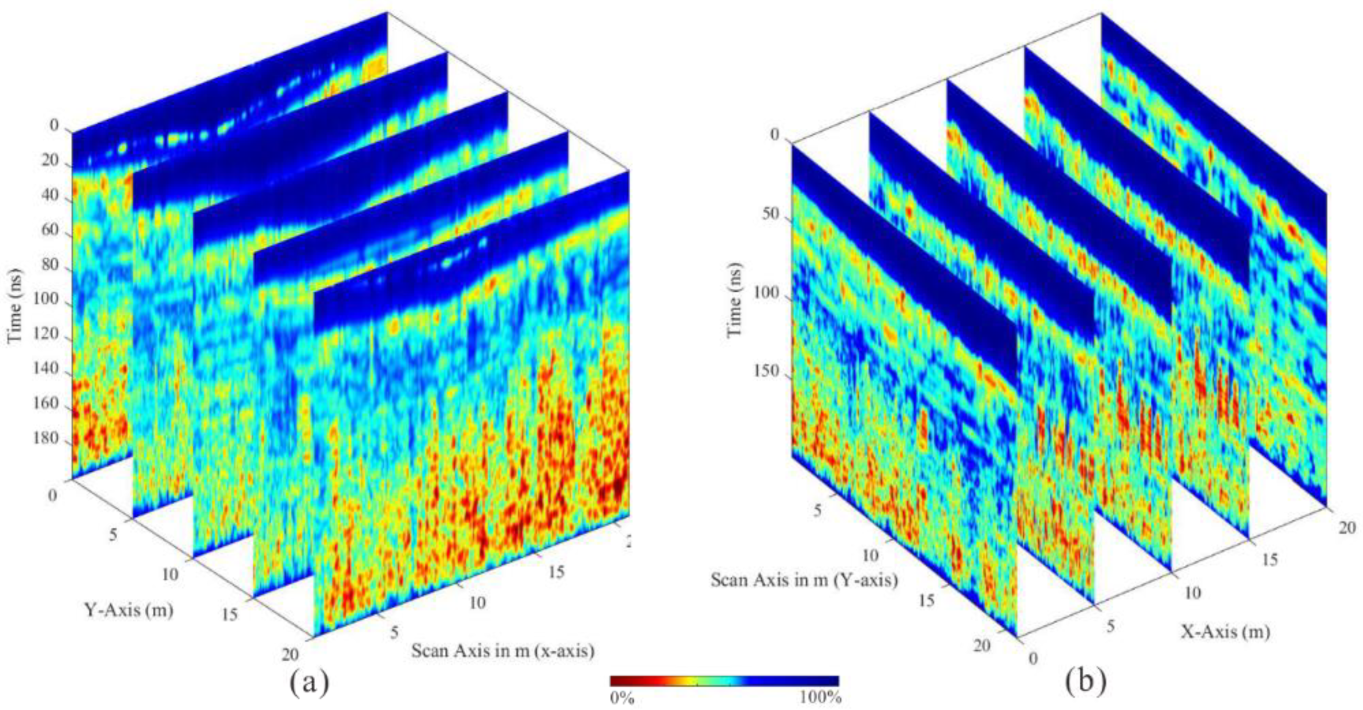
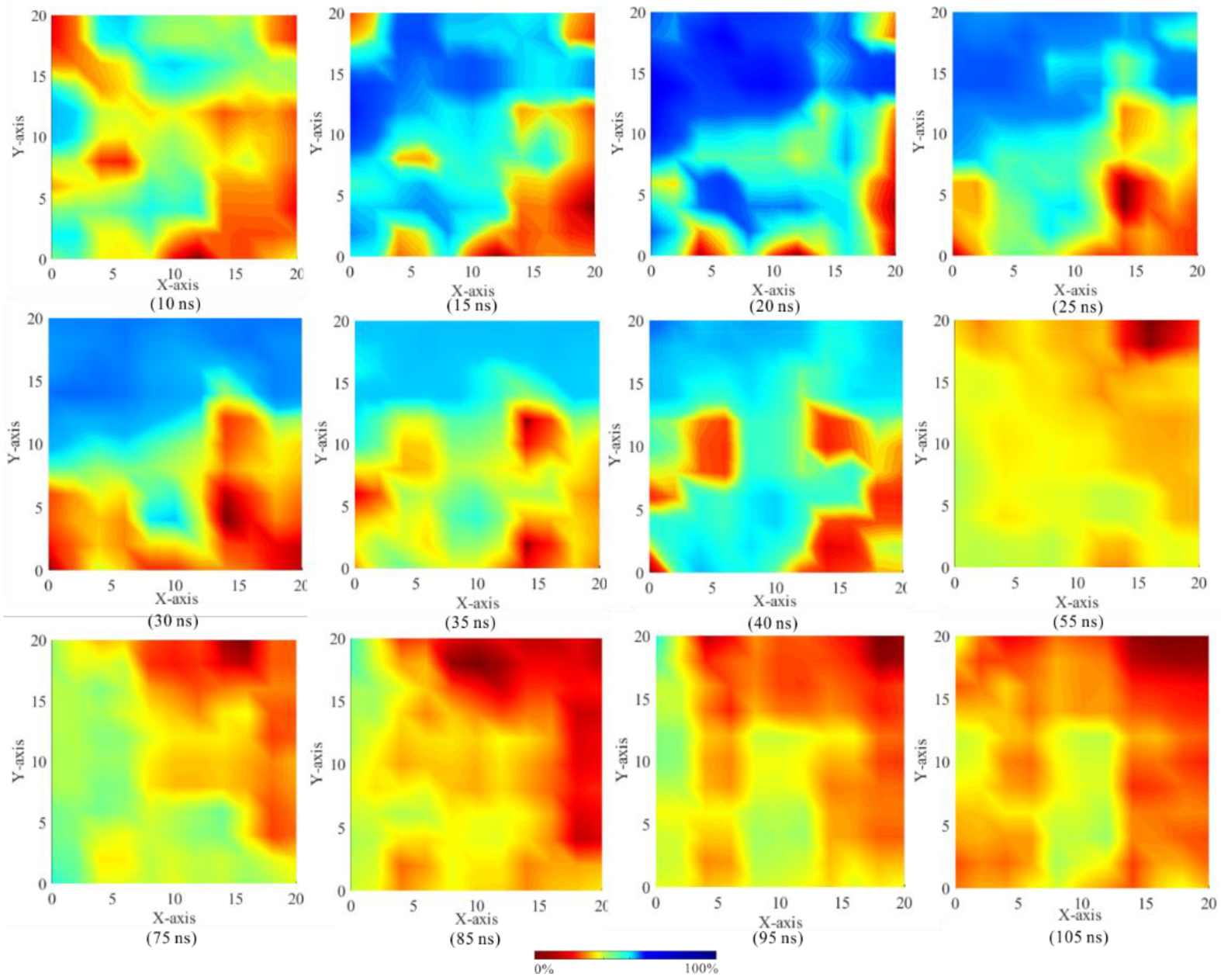
3.2. Relative Water Content Analysis

The water content calculation of thaw-slumping is an important part of GPR. Temperature is the main factor affecting the water content of frozen soil. Figure 21 shows the soil temperature trend profile measured by the vertical and horizontal lines. The surface temperature of the soil is higher, and downward due to the presence of frozen soil, the temperature becomes lower. The black dashed line in Figure 21 shows the trend of temperature change. The black dots display the actual measured temperature value (measured to a depth of 3 m). There is a good correlation between the value of the weighted average frequency attribute (0–1) and the temperature (−1–4 degrees Celsius).

Figure 22 shows the profiles of the sweetness attributes of different survey lines. Blue shows sandy mudstone soils with low water content. Due to the erosion of water, the dielectric constant of sandy mudstone soil with high water content tends to be close to that of wet mudstone. Purple to gray shows sandy mudstone soil with increasing water content.

Figure 23 shows the relative water content 3D profile of different line data. Because in the research of thaw-slumping water content calculation, the main concern area is the fully melted layer, ice-water mixed layer, and ice-bearing layer between 10 and 110 ns. The changing trend of relative water content is consistent with the actual water content change characteristics of the thermal melt landslide. At present, in this landslide area, referring to the actual temperature data, it is found that the calculated relative water content is in line with the actual law in this region. To analyze the release and distribution of water content inside the thaw-slumping from a plane, we performed time slice processing on the data.

Figure 24 shows the time slice characteristics of relative water content at different depths of time. Blue represents high relative water content and red represents low relative water content. Based on the comparison with the actual sample moisture content data (0–1.5 m, six moisture probes), the changing trend of relative water content is consistent with the actual water content change characteristics of the thermal melt landslide. The calculated relative water content can truly reflect the relative size of the soil water of the landslide body.

Before 10 ns, surface soil water loss and crack development, its relative water content is low, and there is local water accumulation. As the depth increases (10–25 ns), the relative water content in the fully melted layer continues to increase, and there are local soil cracks and water loss. In the time depth between 25 and 55 ns, due to the continuous increase of unmelted frozen soil, the relative water content in the ice-water mixed layer gradually decreases with the increase in depth. As the time depth increases (75–105 ns), the relative water content in the ice-bearing layer gradually weakens to a minimum. The profile and plane data of the relative water content show that due to the presence of a large amount of water, the thaw-slumping is most prone to the movement of the landslide body at 15–40 ns. The treatment of thaw-slumping can be accurate to the depth and the plane position with higher relative content.

4. Discussion

Thaw-slumping is widely developed along the Qinghai–Tibet Project. How to manage and repair its development in a targeted manner is the key to ensuring engineering safety and ecological safety. The division of the medium layer inside the landslide is the framework basis for the study of thaw-slumping. Because geological stratification mainly depends on geotechnical analysis and is limited to single-point analysis. GPR data stratigraphic division interpretation not only depends on geological information but also can reflect the change in the dielectric constant of the formation. The division of the media with the same lithology but a different dielectric constant is more detailed. The comprehensive use of GPR data and geological data can more accurately classify the underground media layer of thaw-slumping. Research shows that amplitude and amplitude attenuation can layer the medium well. However, stratification requires the combination of geological and engineering theoretical foundations in frozen soil areas, and the internal structure of a thaw-slumping cannot be judged solely from the electrical properties of electromagnetic waves. In addition, due to the extensive development of water and cracks on the surface of the landslide, ensuring the accuracy and signal-to-noise ratio of radar data collection is also a key guarantee for data analysis. The results of this study show that there is a mixture of ice and water in the internal structure of the landslide. This phenomenon is caused by the cracks on the surface of the landslide and the inhomogeneity of the ablation of frozen soil. The resulting anisotropic characteristics are more likely to cause mechanical instability at the bottom of the thaw-slumping.

Water content calculation and water distribution characteristics are one of the key parameters in the engineering research of thaw-slumping. Although GPR data cannot provide an absolute value of water content. Fortunately, changes in the water content of the soil lead to changes in the electrical properties of the medium, which affects the propagation characteristics of electromagnetic waves. These characteristics can be well reflected in the GPR radar data. Through mathematical analysis and statistics, the electromagnetic wave attribute parameters that are sensitive to water content can be screened. These attribute parameters have certain applicability in a region. In other areas, it is not fully applicable.

In addition, to obtain absolute and accurate water content values, multi-point borehole soil analysis and model-based inversion technology should be combined. By obtaining the structural frame, water content, temperature, and other parameters of the landslide body, a geotechnical numerical model of the landslide body can be constructed. By simulating the mechanical distribution characteristics, the instability research of thaw-slumping bodies will be more in-depth. The GPR should monitor the landslide body for a long time in the same month of each year. Due to the study of the change in the thaw-slumping, the formation of 4D data will have more academic and practical application value.

5. Conclusions

We provide a layer-division method for using the GPR data to carry out thaw-slumping on the Tibetan Plateau. Amplitude analysis and electromagnetic wave amplitude attenuation attributes are used to make a more detailed imaging division of the thaw-slumping. The medium in the thaw-slumping is divided into a finer four-layer structure. They are a fully melted layer, an ice-water mixed layer, an ice-bearing layer, and a low-ice-bearing sand mudstone layer.

To maximize the reduction of the expansion error caused by the participation of noise in the data calculation, the amplitude attribute of the reflection intensity change caused by the change in the dielectric constant of the reaction medium is selected as a parameter for calculating the relative water content. Noise and short-wavelength issues can interfere with the instantaneous frequency analysis, therefore affecting the interpretation of the data. Using weighted average frequency can weaken this effect. The weighted average frequency attribute can reflect temperature change trends, which can be used as another parameter to calculate the relative water content.

Due to the change in soil water content, the soil’s physical properties change. The sweetness attribute can be used to distinguish the changes in soil physical properties caused by changes in water content. The relative water content calculated by combining these attributes is in good agreement with the actual measured value. These methods and results data are valuable for the characterization, evaluation, and treatment of thaw-slumping.

References

1. Wang, Y.; Jin, H.; Li, G. Investigation of the freeze–thaw states of foundation soils in frozen soil areas along the China–Russia Crude Oil Pipeline (CRCOP) route using ground-penetrating radar (GPR). Cold Reg. Sci. Technol. 2016, 126, 10–21. [Google Scholar] [CrossRef]
2. Niu, F.J.; Gao, Z.Y.; Lin, Z.J.; Fan, X.W. Vegetation influence on the soil hydrological regime in frozen soil regions of the Qinghai-Tibet Plateau, China. Geoderma 2019, 354, 113892. [Google Scholar] [CrossRef]
3. Shi, Y.; Niu, F.; Yang, C.; Che, T.; Lin, Z.; Luo, J. Frozen soil presence/absence mapping of the qinghai-tibet plateau based on multi-source remote sensing data. Remote Sens. 2018, 10, 309. [Google Scholar] [CrossRef]
4. Niu, F.J.; Zhang, J.M.; Zhang, Z. Engineering geological characteristics and evaluations of frozen soil in Beiluhe testing field of Qinghai-Tibetan railway. J. Gla. Geo. 2002, 24, 264–269. [Google Scholar]
5. Cheng, G.D. Research on engineering geology of the roadbed in frozen soil regions of Qinghai-Xizang plateau. Quat. Res. 2003, 23, 134–141. [Google Scholar]
6. Niu, F.J.; Lin, Z.J.; Lu, J.H. Characteristics of Roadbed Settlement in Embankment-bridge Transition Section along the Qinghai-Tibet Railway in Frozen soil Regions. Cold Reg. Sci. Technol. 2011, 65, 437–445. [Google Scholar] [CrossRef]
7. Niu, F.J.; Cheng, G.D.; Ni, W.K. Engineering-related slope failure infrozen soil regions of the Qinghai-Tibet Plateau. Cold Reg. Sci. Technol. 2005, 42, 215–225. [Google Scholar] [CrossRef]
8. Yin, G.A. Characteristics of Frozen Soil in Beiluhe Basin of Qinghai-Tibet Plateau and Its Response to Climate Change. Ph.D. Thesis, Chinese Academy of Sciences, Lanzhou, China, 2017. [Google Scholar]
9. Jin, W.D. Research on Slope Stability in Frozen Soil Regions of Qinghai-Tibet Plateau. Ph.D. Thesis, Changan University, Xi’an, China, 2004. [Google Scholar]
10. Lantz, T.; Kokelj, S.V.; Gregel, S.E. Relative impacts of disturbance and temperature: Persistent changes in microenvironment and vegetation in retrogressive thaw slumps. Glob. Change Biol. 2009, 15, 1664–1675. [Google Scholar] [CrossRef]
11. Song, L.; Yang, W.H.; Huang, J.H.; Li, H.P.; Zhang, X.J. GPR utilization in artificial freezing engineering. J. Geophys. Eng. 2013, 10, 034004. [Google Scholar] [CrossRef]
12. Vladov, M.L.; Sudakova, M.S. Ground penetrating radar: From physical fundamentals to high-potential applications. In Teaching Guide; GEOS: Moscow, Russia, 2017; p. 240. (In Russian) [Google Scholar]
13. Brown, J.; Hinkel, K.; Nelson, F. The circumpolar active layer monitoring (CALM) program: Research designs and initial results. Polar Geogr. 2000, 24, 166–258. [Google Scholar] [CrossRef]
14. Hinkel, K.M.; Doolittle, J.A.; Bockheim, J.G.; Nelson, F.E.; Paetzold, R.; Kimble, J.M.; Travis, R. Detection of subsurface frozen soil features with ground penetrating radar, Barrow, Alaska. Permafr. Periglac. Process. 2001, 12, 179–190. [Google Scholar] [CrossRef]
15. Schwamborn, G.; Wagner, D.; Hubberten, H.-W. The use of GPR to detect active layer in young periglacial terrain of Livingston. Island, Maritime Antarctica. Near Surf. Geophys. 2008, 6, 327–332. [Google Scholar] [CrossRef]
16. Sudakova, M.; Sadurtdinov, M.; Skvortsov, A.; Tsarev, A.; Malkova, G.; Molokitina, N.; Romanovsky, V. Using ground penetrating radar for frozen soil monitoring from 2015–2017 at calm sites in the Pechora River delta. Remote Sens. 2021, 13, 3271. [Google Scholar] [CrossRef]
17. Campbell, S.; Affleck, R.T.; Sinclair, S. Ground penetrating radar studies of frozen soil, periglacial, and near-surface geology at McMurdo Station, Antarctica. Cold Reg. Sci. Technol. 2017, 148, 38–49. [Google Scholar] [CrossRef]
18. Luo, J. Study on Instability and Susceptibility Evaluation of Frozen Soil Slope in Qinghai-Tibet Engineering Corrido. Ph.D. Thesis, Chinese Academy of Sciences, Lanzhou, China, 2015. [Google Scholar]
19. Robert, C. Time domain reflectometry method and its application for measuring moisture content in Po20. Measurement 2009, 42, 329–336. [Google Scholar]
20. Weiler, K.W.; Teenhuis, T.S.; Kung, K.S. Comparison of ground penetrating radar and time domain reflectometry as soil water sensors. Soil Sci. Soc. Am. J. 1998, 62, 1237–1239. [Google Scholar] [CrossRef]
21. Grote, K.H.; Ubbard, S.; Rubin, Y. Field-scale estimation of volumetric water content using ground penetrating radar ground wave techniques. Water Resour. Res. 2003, 39, 1–13. [Google Scholar] [CrossRef]
22. Shen, Y.P.; Zuo, R.; Liu, J.K. Characterization and evaluation of frozen soil thawing using GPR attributes in the Qinghai-Tibet Plateau. Cold Reg. Sci. Technol. 2018, 151, 302–313. [Google Scholar] [CrossRef]
23. Wang, Q.; Shen, Y. Calculation and interpretation of ground penetrating radar for temperature and relative water content of seasonal frozen soil in Qinghai-Tibet Platea. Electronics 2019, 8, 731. [Google Scholar] [CrossRef]
24. Zou, D.; Lin, Z.; Yu, S.; Chen, J.; Cheng, G. A new map of frozen soil distribution on the Tibetan plateau. Chn. Phar. Affs. 1997, 11, 1–28. [Google Scholar]
25. Zhao, L. A new map of permafrost distribution on the Tibetan Plateau. Cryosphere 2017, 11, 2527–2542. [Google Scholar] [CrossRef]
26. Wang, S.L. Thaw slumping of Fenghuoshan area along Qinghai-Tibet highway. J. Glaciol. Geocryol. 1990, 12, 63–70. [Google Scholar]
27. Jin, D.W. Study on slope stability in permafrost region of Qinghai-Tibet Plateau. Ph.D. Thesis, Changan University, Xi’an, China, 2004. [Google Scholar]
28. Fu, J.N.; De, W.J.; Wei, M.A. Stability Analysis Methods for Evaluating Landslide of Thaw-slumping in Permafrost Regions. J. Glaciol. Geocryol. 2004, 26, 171–174. [Google Scholar]
29. Warren, C.; Giannopoulos, A.; Giannakis, I. GprMax: Open source software to simulate electromagnetic wave propagation for Ground Penetrating Radar. Comput. Phys. Commun. 2016, 209, 163–170. [Google Scholar] [CrossRef]
30. Topp, G.C.; Davis, J.L.; Annan, A.P. Electromagnetic determination of soil water content: Measurements in coaxial transmission lines. Water Resour. Res. 1980, 16, 574–582. [Google Scholar] [CrossRef]
31. Yee, K.S. Numerical solution of initial boundary value problems involving Maxwell’s equations in isotropic media. IEEE Trans. Antennas Propag. 1996, 14, 302–307. [Google Scholar]
32. Giannakis, I.; Giannopoulos, A.; Warren, C.A. Realistic FDTD Numerical Modeling Framework of Ground Penetrating Radar for Landmine Detection. IEEE J. Sel. Top. Appl. Earth Obs. Remote Sens. 2016, 9, 37–51. [Google Scholar] [CrossRef]
33. Levin, G.G.; Vishnyakov, G.N.; Ilyushin, Y.A. Synthesis of three-dimensional phase images of nanoobjects: Numerical simulation. Opt. Spectrosc. 2013, 115, 938–946. [Google Scholar] [CrossRef]
34. Galagedara, L.W.; Parkin, G.W.; Redman, J.D. An analysis of the ground-penetrating radar direct ground wave method for soil water content measurement. Hydrol. Process. 2003, 17, 3615–3628. [Google Scholar] [CrossRef]
35. Huisman, J.A.; Hubbard, S.S.; Redman, J.D.; Annan, A.P. Measuring soil water content with ground penetrating radar. Vadose Zone J. 2003, 2, 476–491. [Google Scholar] [CrossRef]
36. Di, B.Y.; Kamarudin, M.N. Ground water estimation and water table detection with ground penetrating radar. J. Asian Earth Sci. 2011, 4, 193–202. [Google Scholar] [CrossRef]
37. Seger, M.A.; Nashait, A.F. Detection of water-table by using ground penetration radar. Eng. Technol. J. 2011, 29, 554–566. [Google Scholar]
38. Pyke, K.; Eyuboglu, S.; Daniels, J.J.; Vendl, M.A. controlled experiment to determine the water table response using ground penetrating radar. J. Environ. Eng. Geophys. 2008, 13, 335–342. [Google Scholar] [CrossRef]
39. Ma, F.J.; Lei, S.G.; Yang, S. Study on the relationship between soil moisture content and GPR signal properties. J. Soil Sci. 2014, 45, 809–815. [Google Scholar] [CrossRef]
40. Peng, Z.Y.; Peng, S.P.; Du, W.F. Detection of soil water content using ground penetrating radar average envelope amplitude method. Trans. Chin. Soc. Agric. Eng. 2015, 31, 158–164. [Google Scholar] [CrossRef]
41. Fu, J. Research on shallow soil moisture detection method based on ground penetrating radar technology. Ph.D. Thesis, Anhui University of Technology, Hefei, China, 2022. [Google Scholar]
42. Liu, J. Model experimental study on prediction of subgrade moisture content based on GPR attributes. J. Rai. Sci. Eng. 2018, 15, 2240–2245. [Google Scholar] [CrossRef]
43. Zhao, W.K. Research on Ground Penetrating Radar Attribute Technology and Its Application in Archaeological Investigation. Ph.D. Thesis, Zhejiang University, Hangzhou, China, 2013. [Google Scholar]
44. Schmalz, B.; Lennartz, B.; Wachsmuth, D. Analyses of soil water content variations and GPR attribute distributions. J. Hydrol. 2002, 267, 217–226. [Google Scholar] [CrossRef]
45. Tronicke, J.; Böniger, U. GPR attribute analysis: There is more than amplitudes. First Brk. 2013, 31, 103–108. [Google Scholar] [CrossRef]
46. Niu, J.; Liu, Y.; Jiang, W.; Li, X.; Kuang, G. Weighted average frequency algorithm for Hilbert–Huang spectrum and its application to micro-Doppler estimation. IET Radar Sonar Navig. 2012, 6, 595–602. [Google Scholar] [CrossRef]
47. Gao, J.H.; Wang, Q.; Liu, N.H. Weighted average instantaneous frequency extraction via time-frequency analysis. In Proceedings of the 79th EAGE Conference and Exhibition, Paris, France, 12–15 June 2017. [Google Scholar] [CrossRef]
48. Ogiesoba, O.C. Application of thin-bed indicator and sweetness attribute in the evaluation of sediment composition and depositional geometry in coast-perpendicular subbasins, South Texas Gulf Coast. Interpretation 2017, 5, 87–105. [Google Scholar] [CrossRef]
49. Zheng, J.; Peng, G.; Sun, J.; Zhen, Z. Fusing amplitude and frequency attributes for hydrocarbon detection using 90° phase shift data. Geophys. Prospect. Pet. 2019, 58, 130–138. [Google Scholar]
50. Hart, B.S. Channel detection in 3-D seismic data using sweetness. AAPG Bull. 2008, 92, 733–742. [Google Scholar] [CrossRef]
51. Loughlin, P.J. Comments on the interpretation of instantaneous frequency. IEEE Signal Process. Lett. 1997, 4, 123–125. [Google Scholar] [CrossRef]
Figure 1. The frozen ground distribution on the Qinghai-Tibet Plateau.
Remotesensing 15 02273 g001
Figure 2. Schematic diagram of thaw-slumping hazard.
Remotesensing 15 02273 g002
Figure 3. Thaw-slumping hazard site display: (a) the step-shaped collapse; (b) surface soil cracks; (c) thaw-slumping body; (d) the debris flow and Qinghai–Tibet Project Corridor.
Remotesensing 15 02273 g003
Figure 4. Schematic diagram of measurement network layout: (a) the actual measurement network layout; (b) the plan layout of the survey network (black dashed lines indicate elevation).
Remotesensing 15 02273 g004
Figure 5. Display of acquired data in GSSI RADAN 7 software: (a) Line 1 GPR data profile; (b) 3D GPR data.
Remotesensing 15 02273 g005
Figure 6. Data processing flow chart.
Remotesensing 15 02273 g006
Figure 7. Data analysis and processing diagram: (a) the surface elevation error, background noise, and multiple noise and ringing effects; (b) the grayscale processed data; (c) the color display mode of the raw amplitude signal; (d) the color profile of the processed data.
Remotesensing 15 02273 g007
Figure 8. Spectrum analysis: (a) before processing; (b) after processing; the spectrum burr caused by noise been suppressed (in the red box), ringing effects and multiple interferences are suppressed (red arrow).
Remotesensing 15 02273 g008
Figure 9. Model 1 and simulation data: (a) model diagram; (b) B-scan simulation data; the black arrow shows the location of the layered interface in the model.
Remotesensing 15 02273 g009
Figure 10. Amplitude energy attenuation trend analysis.
Remotesensing 15 02273 g010
Figure 11. Model 2 and simulation data: (a) model diagram; (b) B-scan simulation data; (c) B-scan simulation data in color mode; the white box area is the reflection amplitude of the unthawed frozen soil.
Remotesensing 15 02273 g011
Figure 12. Model 3 and simulation data: (a) model diagram; (b) B-scan simulation data; (c) B-scan simulation data in color mode; the noise caused by obvious surface mud reflection (red box) and unmelted frozen soil reflection (white box).
Remotesensing 15 02273 g012
Figure 13. Model 4 and its parameter values: (a) model diagram; (b) a frozen soil model with different water content parameters.
Remotesensing 15 02273 g013
Figure 14. Simulation data of Model 4: (a) the white box shows ice-water mixed clay (No. 2) radar reflection amplitude region; (b) the white arrows indicate target reflection amplitude; (c) The red dashed line shows the A-scan reflection wave of the target.
Remotesensing 15 02273 g014
Figure 15. The relationship between the average weighted frequency, sweetness, and: (a) dielectric constant; (b) water content.
Remotesensing 15 02273 g015
Figure 16. The GPR grayscale profile from Line 1 to Line 10.
Remotesensing 15 02273 g016
Figure 17. Cracks and unevenness in GPR data.
Remotesensing 15 02273 g017
Figure 18. Amplitude energy attenuation trend analysis from Line 1 to Line 10.
Remotesensing 15 02273 g018
Figure 19. Amplitude B-scan display and layer analysis profiles of Line 1, Line 3, and Line 5: the white arrows indicate strong reflections in the overall weak reflection background of the ice-water mixed layer.
Remotesensing 15 02273 g019
Figure 20. Amplitude display and layer analysis profiles of Line 6, Line 8, and Line 10.
Remotesensing 15 02273 g020
Figure 21. The weighted average frequency attribute profile.
Remotesensing 15 02273 g021
Figure 22. The sweetness attribute profile.
Remotesensing 15 02273 g022
Figure 23. The relative water content 3D profile of different Line data: (a) Line 1–5; (b) Line 6–10.
Remotesensing 15 02273 g023
Figure 24. Relative water content time slice.
Remotesensing 15 02273 g024