MBCNet: Multi-Branch Collaborative Change-Detection Network Based on Siamese Structure

Abstract

The change-detection task is essentially a binary semantic segmentation task of changing and invariant regions. However, this is much more difficult than simple binary tasks, as the changing areas typically include multiple terrains such as factories, farmland, roads, buildings, and mining areas. This requires the ability of the network to extract features. To this end, we propose a multi-branch collaborative change-detection network based on Siamese structure (MHCNet). In the model, three branches, the difference branch, global branch, and similar branch, are constructed to refine and extract semantic information from remote-sensing images. Four modules, a cross-scale feature-attention module (CSAM), global semantic filtering module (GSFM), double-branch information-fusion module (DBIFM), and similarity-enhancement module (SEM), are proposed to assist the three branches to extract semantic information better. The CSFM module is used to extract the semantic information related to the change in the remote-sensing image from the difference branch, the GSFM module is used to filter the rich semantic information in the remote-sensing image, and the DBIFM module is used to fuse the semantic information extracted from the difference branch and the global branch. Finally, the SEM module uses the similar information extracted with the similar branch to correct the details of the feature map in the feature-recovery stage.

1. Introduction

The change-detection method can identify the difference between two remote-sensing images taken at different times and then assign labels to each pixel in the image. Pixels in unchanged areas are labeled 0, while pixels in changed areas are labeled 1. Remote-sensing image change-detection technology has been widely used in urban development planning [1], agricultural surveys [2,3], land management [4,5], and natural disaster assessment [6,7].

The research in the field of change detection can be traced back to 1977 when [8] used differential methods to identify differences in remote-sensing images. Until now, scholars have proposed many methods and made breakthroughs in this field. This paper mainly divides these methods into two categories based on deep learning: traditional methods and change-detection methods in deep learning.

1.1. Traditional Methods

Pixel-based and object-based methods are two subcategories of traditional approaches.

The initial method involves processing the dual-phase remote-sensing images to obtain the difference image. Subsequently, an appropriate threshold is set to segment the difference image, which allows for the determination of both the change region and the invariant region. The most representative processing methods are the difference method [9] and the ratio method [10]. Rawashdeh [11] completed the identification and evaluation of a newly built irrigation area by differentiating all pixels of the image. These methods are easy to implement and execute and have good detection results for images featuring significant changes or particularly low resolution. However, they are not effective in handling images with slightly higher resolution and less significant changes. To address this limitation, researchers have proposed a method that classifies images based on their content and then uses the classification results for change detection. However, this approach leads to a strong correlation between the accuracy of change detection and the accuracy of image-content classification. If the accuracy of image-content classification is not high, the accuracy of the change-detection results will be low, and this method does not fully utilize all the information of the image. Comber [12] first classify an image to obtain a classification object, then cover it with another pixel-based classification result and identify the correct changes in the classification error through expert knowledge. In 2011, Kesikoglu [13] first classified Landsat remote-sensing images and then used the classified results to detect changes. The above two methods only use the spectral information of the image to some extent, ignoring other information of the remote-sensing images, such as shape information and texture information.

In 1995, after Hay [14] proposed the concept of the object, the object-based change-detection method was rapidly developed. The object-based method can use the shape, texture, and other information of the image and rich spatial context information. Therefore, the object-based method is much better than the pixel-based method. Aiming at the characteristic that different targets have different backscattering characteristics, Shi [15] proposed an object-oriented change-detection method for POLSAR images based on the weighted polarization scattering difference. Leichtle [16] applied k-means clustering to distinguish the change region and the invariant region of the image based on principal component analysis. This method can obtain multiple sets of object-based difference features from the image data. Desclee [17] performed a single segmentation of multiple remote-sensing images with region-merging technology to depict objects with statistical characteristics of reflectance difference and marked the corresponding objects as changes using outliers. The above methods can make use of the rich information in the image, but the ability to extract features is insufficient, so the accuracy of change detection is not high enough.

1.2. Change-Detection Method in Deep Learning

Deep learning techniques have advanced rapidly due to the ongoing increase in computer technology [18,19,20,21]. The powerful feature-extraction ability and end-to-end network structure of deep learning methods can be effectively applied to the field of remote-sensing image-change detection. To identify landslide catastrophes, Ding [22] suggested a technique combining texture-change detection and convolutional neural networks. The efficiency and convenience of this method are better than traditional methods. In order to better mine the rich information in the image, Wang [23] proposed an end-to-end neural network framework by combining a sub-pixel hybrid affinity matrix and a two-dimensional convolutional neural network. Zhan [24] proposed a change-detection method based on twin convolutional neural networks and used a weighted contrast loss function to train the method, which can better distinguish the change region from the invariant region of the image. Zhang [25] proposed a joint learning network of spectrum space, which uses a network similar to dual CNN to extract a joint representation of spectrum space, fuses it to represent different information, and then explores potential information through discriminative learning. Liu [26] designed a super-resolution remote-sensing image change-detection network that proposed a module that can overcome the resolution difference between two-time remote-sensing images.

The method mentioned above has demonstrated the effectiveness of using CNN’s feature-extraction ability for remote-sensing analysis, making a breakthrough in the task of change detection. However, as remote-sensing technology continues to improve, the resolution of remote-sensing images will increase. At higher resolutions, the noise problem in dual-time remote-sensing images will become more pronounced [27]. For example, small deviations may occur between the two images caused by differences in the imaging angles [28]. Additionally, differences in the color and brightness caused by changes over time may also exist [29]. In addition to these issues, there are many other challenges that need to be addressed. Therefore, feature extraction is necessary to effectively tackle these challenges. Some existing methods enhance the model’s receptive field by adding additional convolutional layers, thus improving the model’s ability to extract features [30,31,32]. There are also some methods that simply utilize attention mechanisms to enhance the model’s ability to focus on the regions of change in the two images [33,34]. These two methods are inefficient in enhancing the model’s ability to extract features.

1.3. Content of This Article

To address the issue with existing deep learning methods, this paper proposes a multi-branch collaborative network for change detection based on the Siam structure. In the feature-encoding stage, we subdivide the semantically rich feature information within remote-sensing images and construct three branches, the differential branch, global branch, and similar branch, to extract and filter different semantic information. Then, during the feature-decoding stage, we utilize progressive upsampling to fuse the three different kinds of extracted semantic information in order to recover as much of the original image’s overall structure and details as possible. In the difference branch, this paper proposes a cross-scale feature-attention module (CSAM) to pay attention to the information of the changing region in the dual-temporal remote-sensing image. In the global branch, because the concat operation will yield a lot of information, this paper proposes a global semantic filtering module (GSFM) to filter the useful information. Considering that simple fusion will lead to information redundancy, this paper proposes a double-branch information-fusion module (DBIFM) to fuse the obtained differential semantic information and global semantic information. In the process of upsampling recovery, a similarity-enhancement module (SEM) is proposed to supplement the similar semantic information extracted from the similar branch into the recovered image and correct the edge details. At the bottom of the network, we use the improved pyramid pooling module (PPM) [35] to extract similar semantic information at the bottom. The complete network consists of many millions of parameters in a complex architecture. It uses ResNet as a backbone and features three branches and five modules.

The main contents of this paper can be summarized as the following four points:

1.

A multi-branch collaborative change-detection network based on Siamese structure is proposed.

2.

Previous deep learning approaches do not adequately consider various types of semantically meaningful information in remote-sensing images, leading to limitations in their ability to extract features. Some more-traditional methods are unable to differentiate between the changed and invariant regions, let alone identify the changing region. The network continuously extracts different levels of differential semantic information, global semantic information, and similar semantic information through three branches and continuously aggregates different levels of differential semantic information, global semantic information, and similar semantic information in the process of upsampling. It distinguishes the changing area and the invariant area and pays attention to the edge details as much as possible.

3.

For the difference semantic information, global semantic information, and similar semantic information in the three branches, a cross-scale feature-attention module (CSAM), global semantic filtering module (GSFM), double-branch information-fusion module (DBIFM) and similarity-enhancement module (SEM) are proposed. The four modules independently and selectively integrate multi-level difference information.

4.

Ablation experiments and comparative experiments were performed on the self-built BTRS-CD dataset and the public LEVIR-CD dataset. The ablation experiments show that each module of MHCNet can help the whole network to complete the change-detection task. The comparative experiments show that MHCNet has a higher performance in change-detection tasks.

2. Methods

Previous research has shown that CNNs deliver an excellent performance in segmentation tasks [36]. Additionally, the dual-branch weight-sharing structure of Siamese networks can extract semantically rich information from two images separately. Leveraging the above advantages, we propose MHCNet, a approach that combines Siamese networks with CNNs. Although the change-detection task only requires identification of the changed and invariant regions, the changed region still contains a significant amount of semantically meaningful information pertaining to various types of terrain. This places greater demands on the network model’s ability to extract features. Therefore, we choose three operations to construct the difference branch, the global branch, and the similar branch to further refine and extract the different information of the dual-temporal remote-sensing image. These three operations are: Through the subtraction operation, the extracted feature maps are directly subtracted, and the obtained feature maps have sufficient difference semantic information. The difference branch further extracts this feature map, the concat operation stacks the extracted feature maps on the channel dimension, and the obtained feature maps have various rich semantic information, mainly acting on the global branch. In addition, the extracted feature maps are directly added, and the obtained feature maps have a large number of similar semantic information corresponding to similar branches.

Figure 1 depicts the overall architecture of the MHCNet proposed in this paper, which consists of a backbone network and four modules. Each layer of ResNet-34 contains different levels of semantic information, which helps us to quickly extract multi-scale information, and the residual structure of ResNet-34 can prevent the network from being too deep. Therefore, we use ResNet-34 with two common parameters as the backbone network of change detection. The four modules are the cross-scale feature-attention module (CSAM), global semantic filtering module (GSFM), double-branch information-fusion module (DBIFM), and similarity-enhancement module (SEM). In the feature-encoding phase, two ResNet-34s with common parameters are used to downsample the dual-time remote-sensing image and obtain four different levels of semantic information. In the feature-decoding phase, the cross-scale feature-attention module (CSAM) focuses on the features after the subtraction operation and optimizes the ability of the difference branch to extract the difference semantic information. The global semantic filtering module (GSFM) improves the efficiency of feature extraction for the rich semantic information after the concat operation. The double-branch information-fusion module (DBIFM) is a weighted aggregation of the difference semantic information extracted using the cross-scale feature-attention module (CSAM) and the global semantic information extracted using the global semantic filtering module (GSFM). The similarity-enhancement module (SEM) extracts similar semantic information after the subtraction operation, which is used to restore the image in upsampling and correct the edge of the image.

2.1. Cross-Scale Feature-Attention Module (CSAM)

For bi-temporal remote-sensing images containing a variety of ground object information, the difference semantic information it contains is also various, which requires the network to have a higher ability to extract features [37]. Therefore, we use the subtraction operation to construct the difference branch to increase the network’s capacity to extract the difference semantic information. This operation directly subtracts the feature maps extracted using ResNet-34 with two common parameters, and the further obtained feature maps contain rich difference semantic information, which is strongly related to the change area we need to identify, but this difference semantic information contains a lot of redundant information. In addition, the deep features have rich semantic information, which is very beneficial to restore the edge information of the object [38], while shallow features have rich global information, which is beneficial to restore the overall contour of the object. Considering the above two points, we propose a cross-scale feature-attention module (CSAM) to optimize the ability of the difference branch to extract the difference semantic information. At the same time, the difference semantic information of each level and the difference semantic information of the previous level guide each other to obtain better difference semantic information. The design of the CSAM module draws on BiseNetv2 [39].

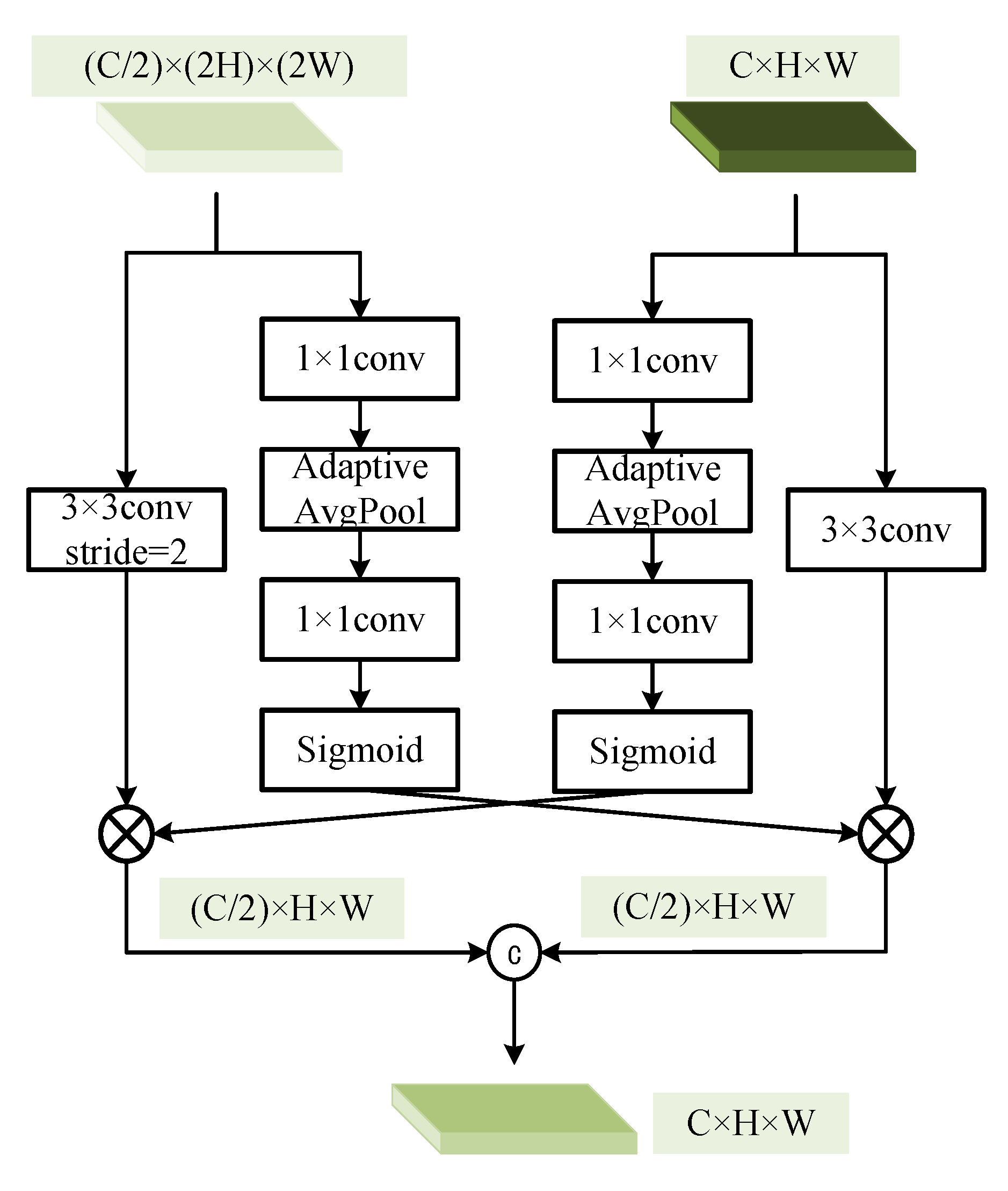
Figure 2 depicts the module’s structure. The module has two inputs $f_{\mathrm{low}}\in R^{\frac{\mathrm{C}}{2}\times 2\mathrm{H}\times 2\mathrm{W}}$ and $f_{\mathrm{high}}\in R^{\mathrm{C}\times 2\mathrm{H}\times 2\mathrm{W}}$, where C, H, and W represent the number of channels and the height and width of the feature map, respectively. For low-level features, we use a 3 × 3 convolution with a step size of 2 to further extract the features, so that they have the same scale as the high-level features. In addition, we also use another branch to weight them to the high-level features that have been further extracted. For high-level features, we use a 3 × 3 convolution with doubling the number of channels to further extract the features, so that they have the same number of channels as the low-level features. In addition, we also weight it by another branch to further extract the low-level features. The following is the calculation formula for the aforementioned process:

$$f_{\mathrm{out}1}=f_2{1}^{3\times 3}\left(f_{\mathrm{low}}\right)\otimes \mathrm{S}\left(f_1{1}^{1\times 1}\left(\mathrm{A}\left(f_1{2}^{1\times 1}\left(f_{\mathrm{high}}\right)\right)\right)\right)$$

(1)

$$f_{\mathrm{out}2}=f_1{2}^{3\times 3}\left(f_{\mathrm{high}}\right)\otimes \mathrm{S}\left(f_1{1}^{1\times 1}\left(\mathrm{A}\left(f_1{1}^{1\times 1}\left(f_{\mathrm{low}}\right)\right)\right)\right)$$

(2)

$$f_{\mathrm{out}}=\mathrm{C}\left(f_{\mathrm{out}1},f_{\mathrm{out}2}\right)$$

(3)

In the above three formulas, ⊗ represents matrix multiplication; $f_2{1}^{3\times 3}(·)$ represents a convolutional layer consisting of a two-dimensional convolution, a batch normalization, and a Relu function, where 3 × 3 in the superscript represents a convolution kernel of 3, and 2 and 1 in the subscript represent steps of 2 and the number of channels 1 times the original, respectively; $f_1{2}^{3\times 3}(·)$ represents a convolutional layer consisting of a two-dimensional convolution, a batch normalization, and a Relu function, where 3 × 3 in the superscript represents a convolution kernel of 3, and 1 and 2 in the subscript represent steps of 1 and the number of channels 1/2 times the original, respectively; $f_1{2}^{1\times 1}(·)$ represents a convolutional layer consisting of a two-dimensional convolution, a batch normalization, and a Relu function, where 1 × 1 in the superscript represents a convolution kernel of 1, and 1 and 2 in the subscript represent steps of 1 and the number of channels 1/2 times the original, respectively; $f_1{1}^{1\times 1}(·)$ represents a convolutional layer consisting of a two-dimensional convolution, a batch normalization, and a Relu function, where 1 × 1 in the superscript represents a convolution kernel of 1, and 1 and 1 in the subscript represent steps of 1 and the number of channels 1 times the original; $\mathrm{S}\left(·\right)$ represents the sigmoid activation function; and $\mathrm{C}(·,·)$ represents the stacking operation of two feature maps on the channel dimension.

2.2. Global Semantic Filtering Module (GSFM)

The concat operation we introduced in the global branch is to stack the various levels of features extractedusingby ResNet-34 [40] with two common parameters on the channel dimension to obtain the global semantic information. Although the concat operation can completely retain the two parts of the extracted semantic information, it ignores the previous relationship between the two. In addition, the extracted rich semantic information can be classified not only into semantic information such as factories, farmland, roads, buildings, and mining areas, but also into semantic information of changing areas and semantic information of unchanged areas. However, for the two-category change-detection task, we only need to focus on one of the semantic information sets. Therefore, it is evident that using the concat operation would result in information redundancy, which will affect the accuracy of the predictions and must be avoided. Considering the above two points, we propose a global semantic filtering module (GSFM) to optimize the ability of the global branch to extract information and avoid the above two shortcomings. The specific way is to extract and strengthen the connection between the two parts of the semantic information through channel attention and location attention with residual structure and then filter out the global semantic information of the change area we focus on as completely as possible through the convolution layer. The design of the GSFM module draws on Cbam [41].

The input of the module is set to $f_{\mathrm{cat}}\in R^{2\mathrm{C}\times \mathrm{H}\times \mathrm{W}}$. The structure diagram of the module is primarily separated into two sections, as shown in Figure 3. In the first part, first, we extract two different channel information sets of C × 1 × 1 using global average pooling and global maximum pooling, respectively, and sum them. Then, the results are entered into the upper and lower 1 × 1 convolutions, respectively, and then the sum of the results is sent to the sigmoid activation function to obtain the weighting coefficient. The weighting coefficient is directly multiplied by $f_{\mathrm{cat}}$ and then added to $f_{\mathrm{cat}}$. Finally, the feature $f_{\mathrm{out}1}$ that screens the channel features is obtained. In the second part, we first obtain two feature maps with a size of 1 × H × W on the channel dimension of $f_{\mathrm{out}1}$ using mean and max operations, respectively. Then, the two images are stacked on the channel dimension and then fed into a 1 × 1 convolution to obtain a weighted coefficient of 1 × H × W. The weighted coefficient is directly multiplied by the $f_{\mathrm{out}1}$ matrix $f_{\mathrm{out}2}$, and then $f_{\mathrm{out}1}$ and addition are performed. The feature $f_{\mathrm{out}2}$ that filters the channel features is obtained. Finally, $f_{\mathrm{out}2}$ is fed into a 3 × 3 convolution for extraction to obtain the final output $f_{\mathrm{out}}$. The following is the calculation formula for the aforementioned process:

$$f_{\mathrm{out}1}=f_{\mathrm{cat}}+f_{\mathrm{cat}}\otimes \mathrm{S}\left(f_1{1}^{1\times 1}\left(\mathrm{A}\left(f_{\mathrm{cat}}\right)+\mathrm{M}\left(f_{cat}\right)\right)+f_1{1}^{1\times 1}\left(\mathrm{A}\left(f_{\mathrm{cat}}\right)+\mathrm{M}\left(f_{\mathrm{cat}}\right)\right)\right)$$

(4)

$$f_{\mathrm{out}2}=f_{\mathrm{out}1}+f_{\mathrm{out}1}\otimes f_1{1}^{1\times 1}\left(\mathrm{mean}\left(f_{\mathrm{out}1}\right)+max\left(f_{\mathrm{out}1}\right)\right)$$

(5)

$$f_{\mathrm{out}}=f_1{2}^{3\times 3}\left(f_{\mathrm{out}2}\right)$$

(6)

In the above three formulas, ⊗ represents matrix multiplication; $f_1{1}^{1\times 1}(·)$ represents a convolutional layer consisting of a two-dimensional convolution, a batch normalization, and a Relu function, where 1 × 1 in the superscript represents a convolution kernel of 1, and 1 and 1 in the subscript represent steps of 1 and the number of channels 1 times the original; $f_1{2}^{3\times 3}(·)$ represents a convolutional layer consisting of a two-dimensional convolution, a batch normalization, and a Relu function, where 3 × 3 in the superscript represents a convolution kernel of 3, and 1 and 2 in the subscript represent steps of 1 and the number of channels 1/2 times the original; $\mathrm{mean}(·)$ represents the function that averages the features in the channel dimension; and $\max (·)$ represents the function that takes the maximum value of the feature in the channel dimension.

2.3. Double-Branch Information-Fusion Module (DBIFM)

Through the two branches of the differential branch and the global branch, we obtain the differential semantic information focusing on the changing region and the global semantic information focusing on the changing region of different features. These two information subsets can constrain the model to accurately determine the change area as much as possible, so we need to efficiently fuse these two different semantic information sets. We propose the double-branch information-fusion module to fuse the two information sets to successfully assess the change area because simple addition, cat, and convolution fusion cannot fully utilize the information and may compromise the information integrity.

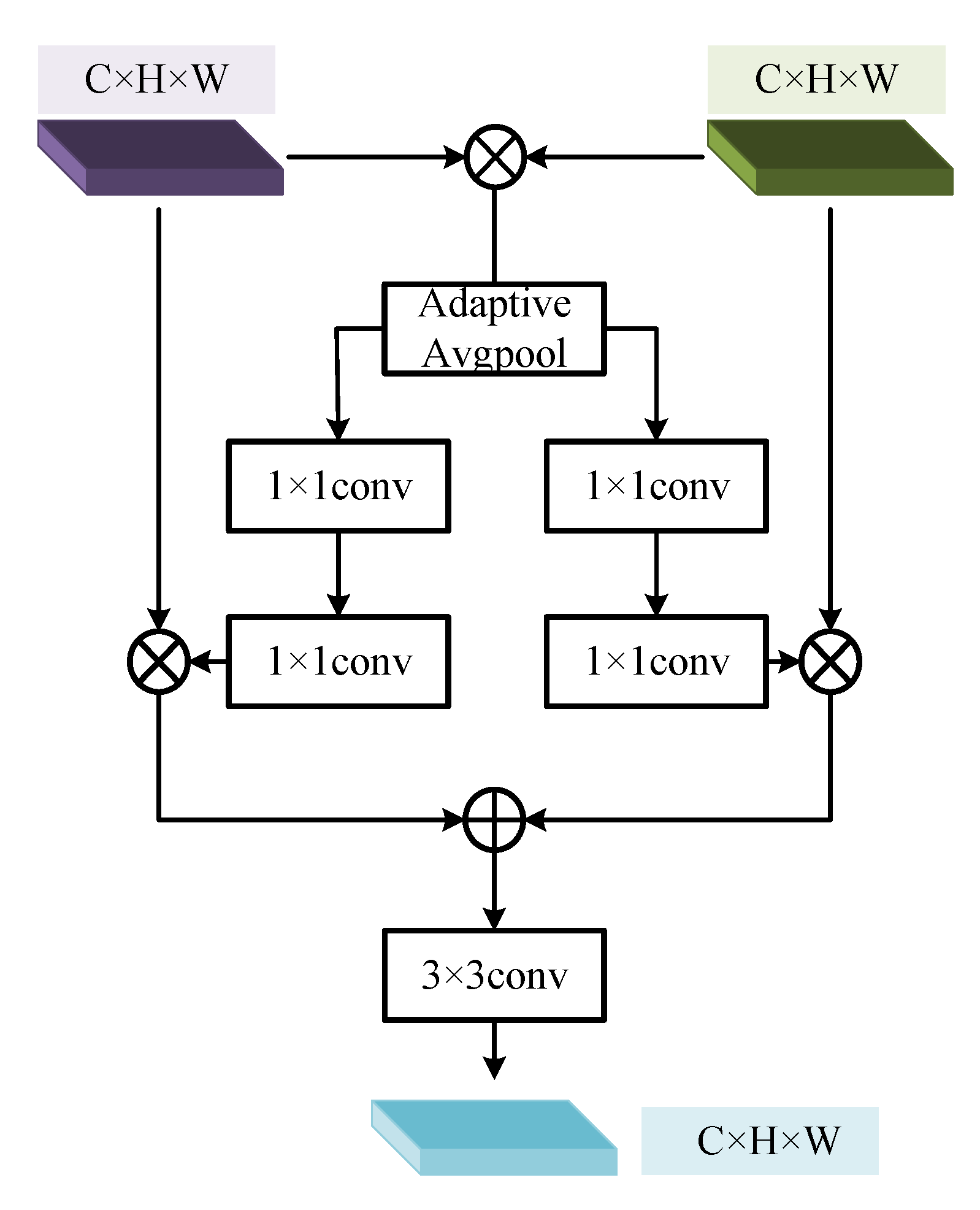
The structure of the double-branch information-fusion module is shown in Figure 4, and the feature maps of the final output of the similar branch and the global branch are received at the same time. Therefore, there are two inputs set to $f_{\mathrm{sub}}\in R^{\mathrm{C}\times \mathrm{H}\times \mathrm{W}}$ and $f_{\mathrm{cat}}\in R^{\mathrm{C}\times \mathrm{H}\times \mathrm{W}}$. Firstly, matrix multiplication is performed on $f_{\mathrm{sub}}$ and $f_{\mathrm{cat}}$, and then the weighting coefficients with a size of C × 1 × 1 are obtained using global average pooling. Then, the weighting coefficients that are consistent with the two semantics are learned by two branches composed of two 1 × 1 convolutions. After that, the two weighting coefficients are multiplied with $f_{\mathrm{sub}}$ and $f_{\mathrm{cat}}$, respectively. Finally, the obtained results are added to the 3 × 3 convolution to obtain the final output feature. The following is the calculation formula for the aforementioned process:

$$f_{\mathrm{out}1}=f_{\mathrm{sub}}\otimes f_1{1}^{1\times 1}\left(f_1{1}^{1\times 1}\left(\mathrm{A}\left(f_{\mathrm{sub}}\otimes f_{\mathrm{cat}}\right)\right)\right)$$

(7)

$$f_{\mathrm{out}2}=f_{\mathrm{cat}}\otimes f_1{1}^{1\times 1}\left(f_1{1}^{1\times 1}\left(\mathrm{A}\left(f_{\mathrm{sub}}\otimes f_{\mathrm{cat}}\right)\right)\right)$$

(8)

$$f_{\mathrm{out}}=f_1{1}^{3\times 3}\left(f_{\mathrm{out}1}+f_{\mathrm{out}2}\right)$$

(9)

In the above three formulas, ⊗ represents matrix multiplication; $f_1{1}^{1\times 1}(·)$ represents a convolutional layer consisting of a two-dimensional convolution, a batch normalization, and a Relu function, where 1 × 1 in the superscript represents a convolution kernel of 1, and 1 and 1 in the subscript represent steps of 1 and the number of channels 1 times the original; and $f_1{1}^{3\times 3}(·)$ represents a convolutional layer consisting of a two-dimensional convolution, a batch normalization, and a Relu function, where 3 × 3 in the superscript represents a convolution kernel of 3, and 1 and 1 in the subscript represent steps of 1 and the number of channels 1 times the original.

2.4. Similarity-Enhancement Module (SEM)

The difference branch and global branch, as well as the cross-scale feature-attention module (CSAM), global semantic filtering module (GSFM), double-branch information-fusion module (DBIFM) can help the model to accurately determine the change area as much as possible, but there may be missed detection and false detection. Therefore, we design a similar branch separately, extract similar semantic information through the similar branch to verify the accuracy of the change area detection from the unchanged area, and correct the missed detection and false detection. In the similar branch, we introduce the addition operation, which directly adds the features extracted using ResNet-34 with two common parameters to obtain similar semantic information. In order to verify whether the change area is accurate and correct the missed detection and false detection, we designed a similarity-enhancement module (SEM) in the feature-decoding process.

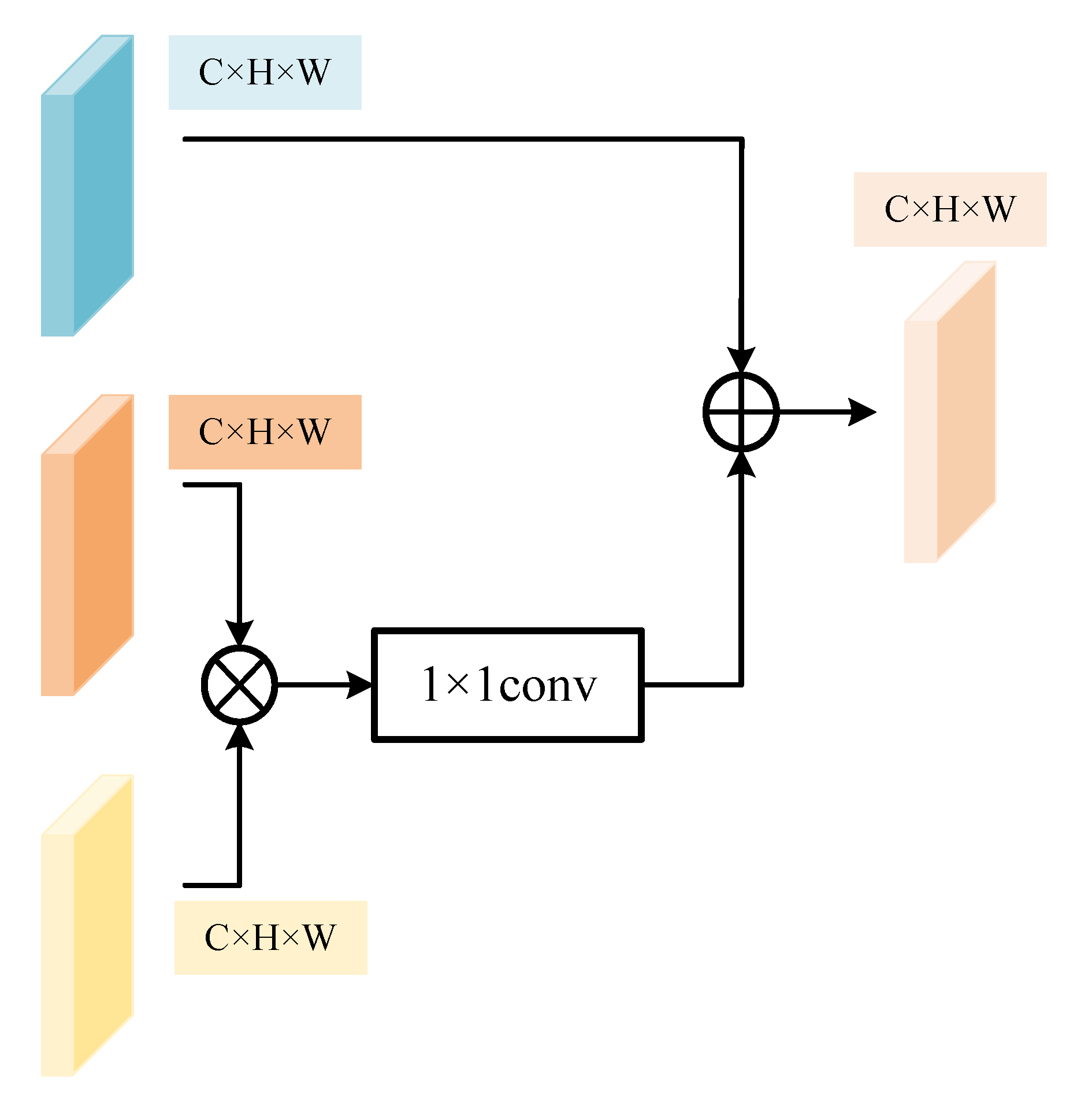
The structure of the similarity-enhancement module (SEM) is shown in Figure 5. This module has a total of three inputs, which are the recovering feature $f_1\in R^{\mathrm{C}\times \mathrm{H}\times \mathrm{W}}$, the feature $f_2\in R^{\mathrm{C}\times \mathrm{H}\times \mathrm{W}}$ with similar semantic information obtained from the similar branch, and the output feature $f_3\in R^{\mathrm{C}\times \mathrm{H}\times \mathrm{W}}$ obtained using the double-branch information-fusion module. First, $f_1$ and $f_2$ are matrix-multiplied, sent to a 1 × 1 convolution, and then added to $f_3$ to obtain the output. The following is the calculation formula for the aforementioned process:

$$f_{\mathrm{out}1}=f_1{1}^{1\times 1}\left(f_1\otimes f_2\right)$$

(10)

$$f_{\mathrm{out}}=f_{\mathrm{out}1}+f_3$$

(11)

In the above two formulas, ⊗ represents matrix multiplication and $f_1{1}^{1\times 1}(·)$ represents a convolutional layer consisting of a two-dimensional convolution, a batch normalization, and a Relu function, where 1 × 1 in the superscript represents a convolution kernel of 1, and 1 and 1 in the subscript represent steps of 1 and the number of channels 1 times the original.

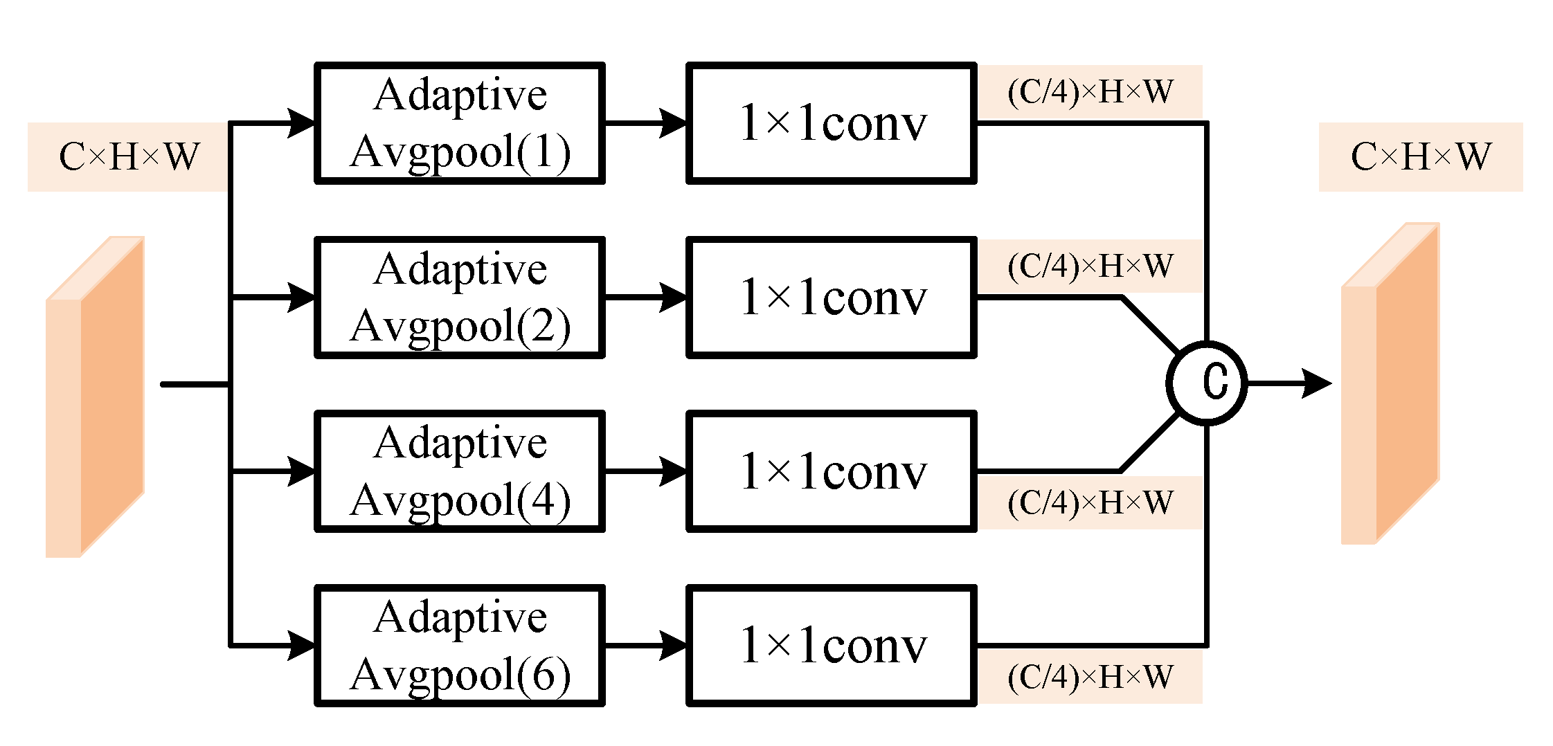
In addition, we improve the pyramid pooling module (PPM) and place it at the bottom layer to further extract the similar semantic information obtained using the addition operation. The extracted features are directly involved in the decoding process. The improved pyramid pooling module (PPM) is shown in Figure 6.

The input of the improved pyramid module (PPM) is the similar semantic information $f\in R^{\mathrm{C}\times \mathrm{H}\times \mathrm{W}}$ at the bottom. First, the global average pooling of four different pooling kernels is used to extract features of different scales, then 1 × 1 convolution is used for dimensionality reduction, and finally they are stacked together for output. The following is the calculation formula for the aforementioned process:

$$f_{\mathrm{out}}=C\left(f_1{4}^{1\times 1}\left({\mathrm{A}}^1\left(f\right)\right),f_1{4}^{1\times 1}\left({\mathrm{A}}^2\left(f\right)\right),f_1{4}^{1\times 1}\left({\mathrm{A}}^4\left(f\right)\right),f_1{4}^{1\times 1}\left({\mathrm{A}}^6\left(f\right)\right)\right)$$

(12)

In the above formulas, $f_1{4}^{1\times 1}(·)$ represents a convolutional layer consisting of a two-dimensional convolution, a batch normalization, and a Relu function, where 1 × 1 in the superscript represents a convolution kernel of 1, and 1 and 1 in the subscript represent steps of 1 and the number of channels 1/4 times the original. ${\mathrm{A}}^{\mathrm{a}}(·)$ represents a two-dimensional global average pooling with a pooled kernel size a.

2.5. Summary at the End of the Chapter

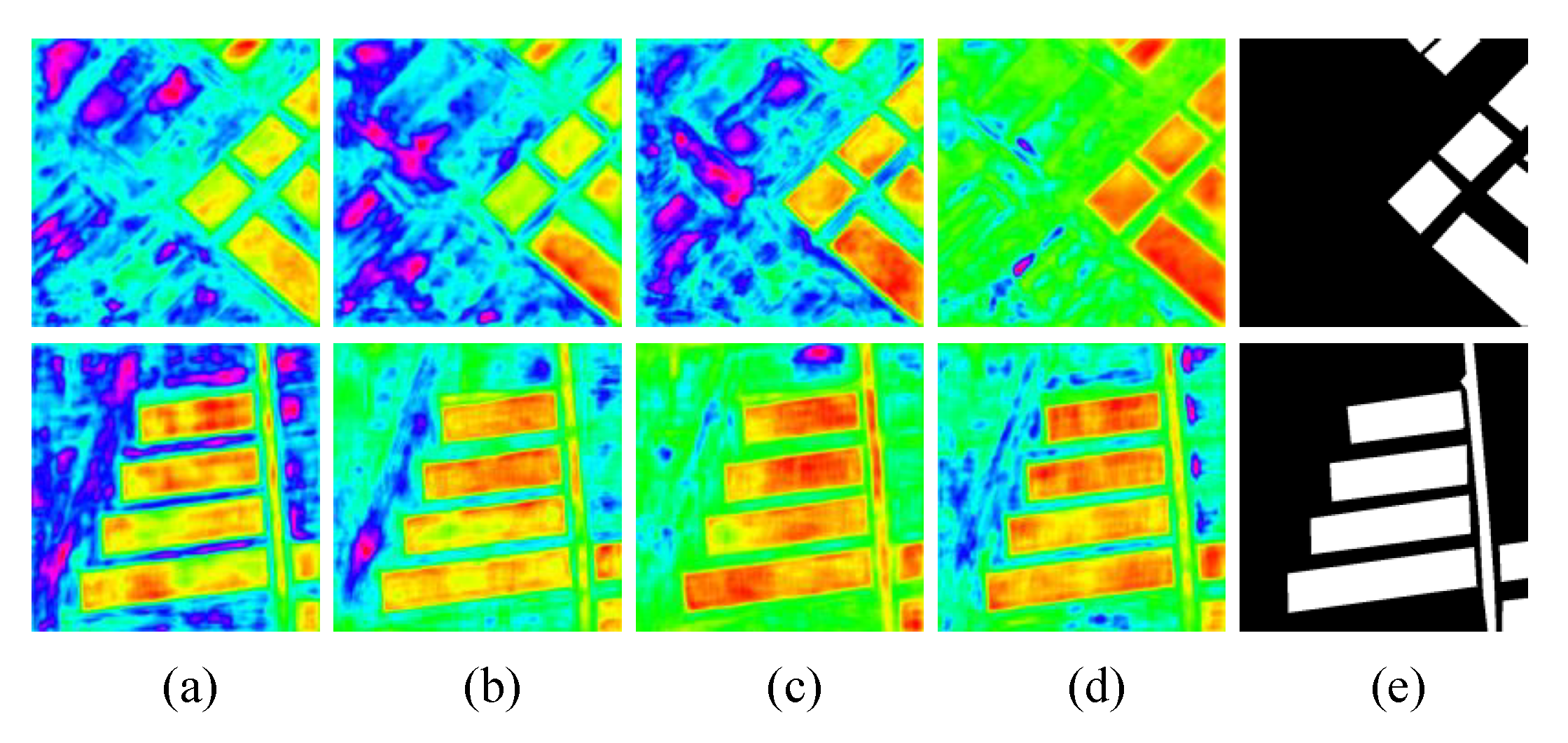
In this chapter, we first provide a detailed introduction of the overall framework of MHCNet. Subsequently, we discuss the strengths and weaknesses of constructing different branches, global branches, and similar branches. Then, we propose a cross-scale feature-attention module (CSAM), a global semantic filtering module (GSFM), and a similarity-enhancement module (SEM) to optimize the advantages and disadvantages of the three branches. We also propose a double-branch information-fusion module (DBIFM) to weight and fuse two different semantic information sources. Finally, we improve the pyramid module at the bottom to improve the role of the similar branches. In addition, we visualized feature extraction at each stage of the model. The specific results are shown in Figure 7.

3. Dataset

We created the BTRS-CD dataset to demonstrate the effectiveness of our approach. Additionally, we also used the LEVIR-CD dataset in our work [30].

3.1. BTRS-CD Dataset

Google Earth’s global geomorphological image is integrated from satellite images and aerial data. Users can obtain satellite images captured using remote-sensing technology at any time around the world free of charge. The BTRS-CD dataset built in this paper is taken from Google Earth. We collected 3520 pairs of 512 × 512 dual-time remote-sensing photos, including 2850 and 570 images in the training and test sets, respectively. All dual-date satellite images used in this study were captured from 664 time points in eastern and central China between 2010 and 2019. These images cover 659 different objects and their surrounding environments, with a coverage area of approximately 3 square kilometers per image. The following is the link to the dataset: https://pan.baidu.com/s/1wph-EHhU16eDdAXasVDhhg?pwd=014t (accessed on 28 February 2023). The publication date of this article is 11 April 2023.

High-quality datasets are essential for improving the robustness and prediction accuracy of the model. Therefore, we developed the following four criteria to help us produce high-quality datasets:

1.

The entire dataset should contain a large number of changed regions.

2.

Human-induced geomorphological changes, such as the expansion of roads in fertile land, the conversion of forests into factories, the expansion and reconstruction of urban buildings, the diversion of rivers, and the return of farmland to forests, can lead to changed areas in remote-sensing images. Therefore, the dataset should include as many of these geomorphological changes as possible.

3.

Seasonal geomorphological changes can also lead to changes in remote-sensing images, such as significant changes in winter and summer broad-leaved forest and river ebb and flow.

4.

Completely rely on manual tagging to turn the most accurate change-area information into a label map in the dataset.

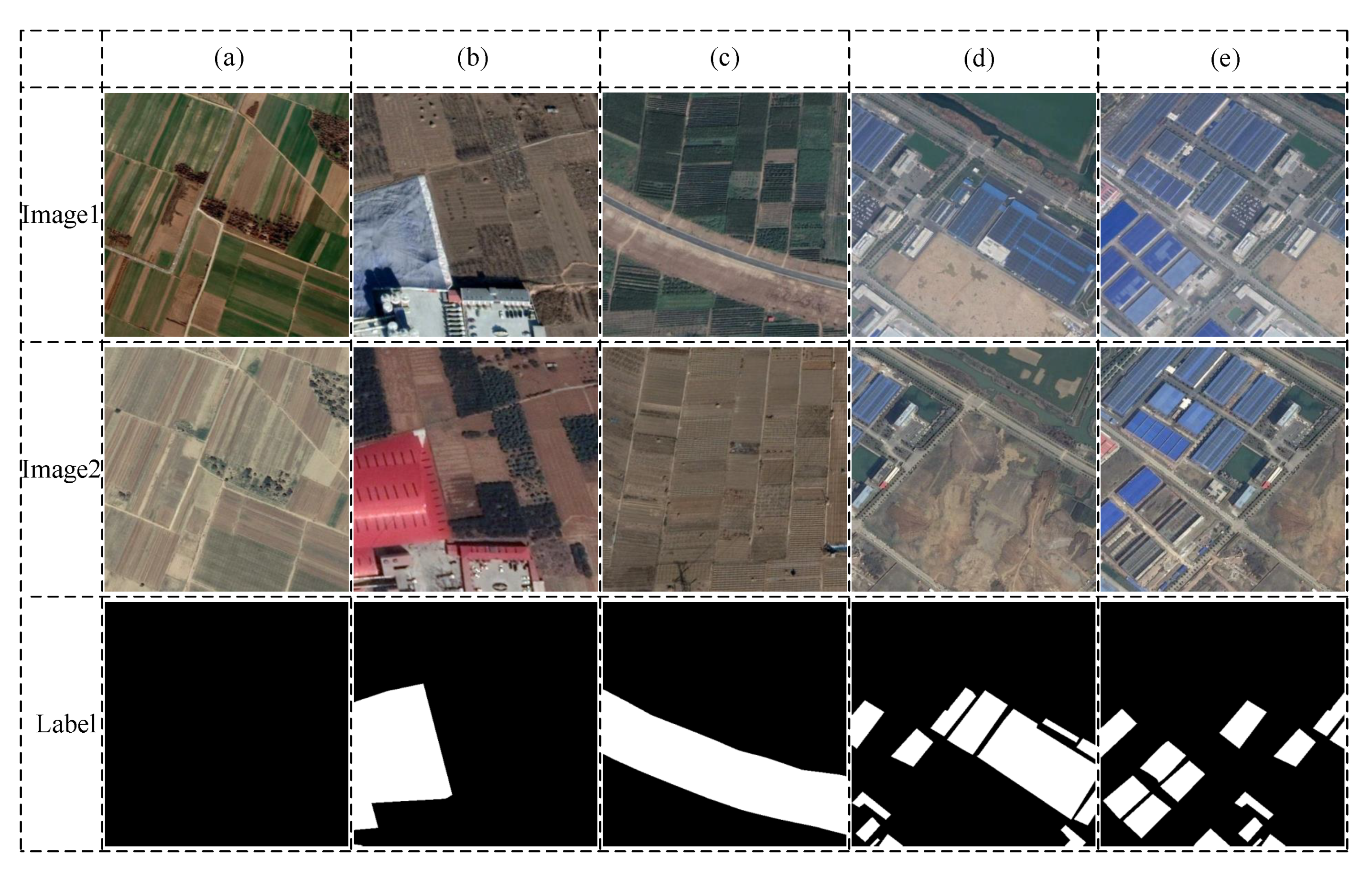
Figure 8 shows a sample of the dataset showing several types of change regions. The dataset includes various types of changes, such as scattered housing reconstruction, clustered factory buildings, irregular roads, and changes caused by large factory construction. Additionally, the dataset also includes many pairs of dual-time remote-sensing images that do not contain any change areas, but exhibit differences in brightness and color due to different shooting times.

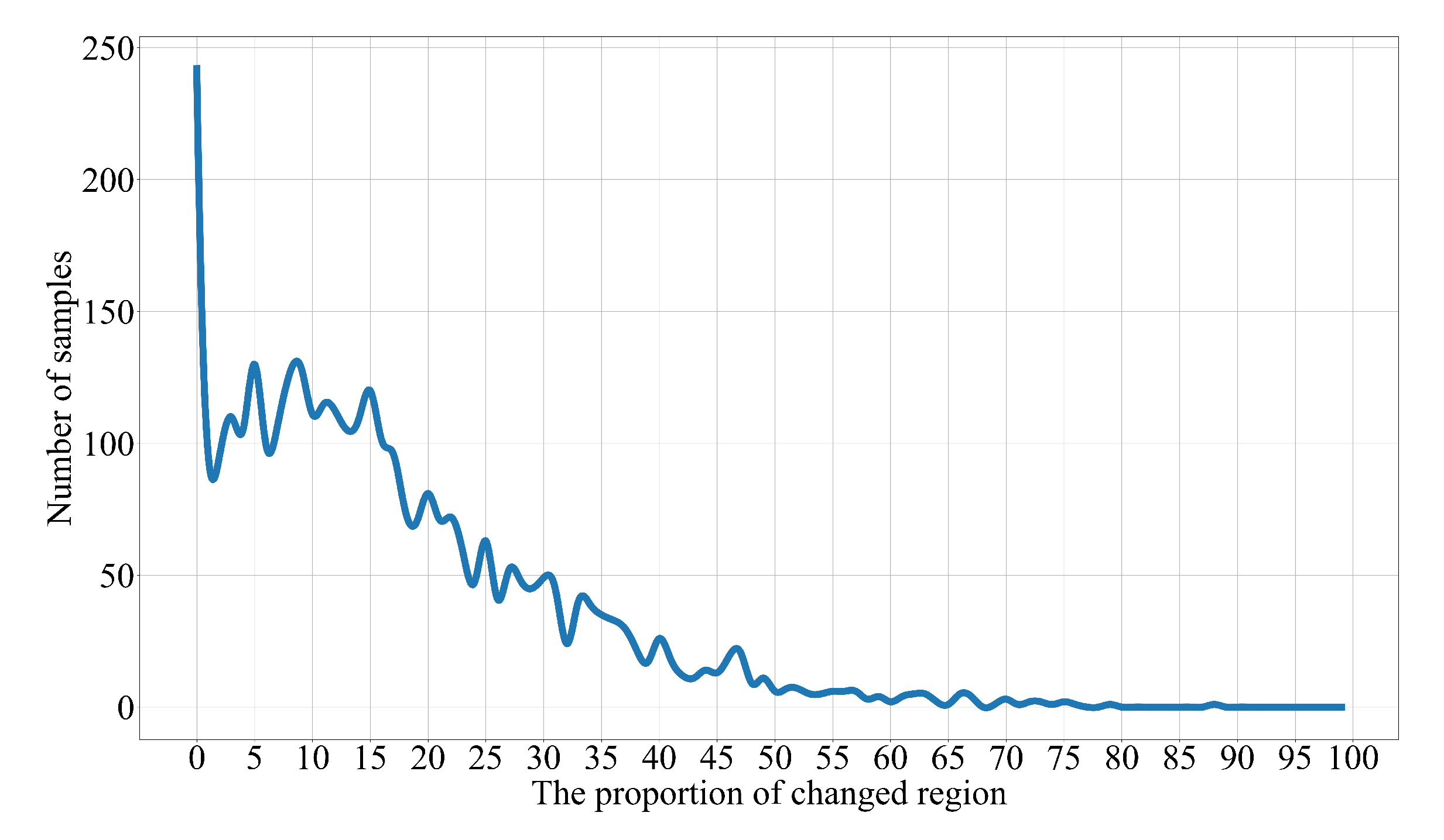
The TRS-CD dataset’s proportion distribution map for the change area is shown in Figure 9. There are more dual-time remote-sensing images with a change area of 0–60% in the dataset.

3.2. LEVIR-CD Dataset

The LEVIR-CD dataset is based on Google Earth global images from 2002 to 2018 in Texas. It consists of 637 pairs of 1024 × 1024 dual-time remote-sensing images. It has the following three characteristics:

1.

The entire dataset covers a time span of 5 to 14 years; thus, the remote-sensing image includes a significant number of areas that have undergone changes.

2.

In terms of spatial coverage, the remote-sensing images from the entire dataset were collected from more than 20 distinct regions across Texas, encompassing a variety of settings such as residential areas, apartments, vegetated areas, garages, open land, highways, and other locations.

3.

The dataset takes into account seasonal and illumination changes, which are crucial factors for developing effective algorithms.

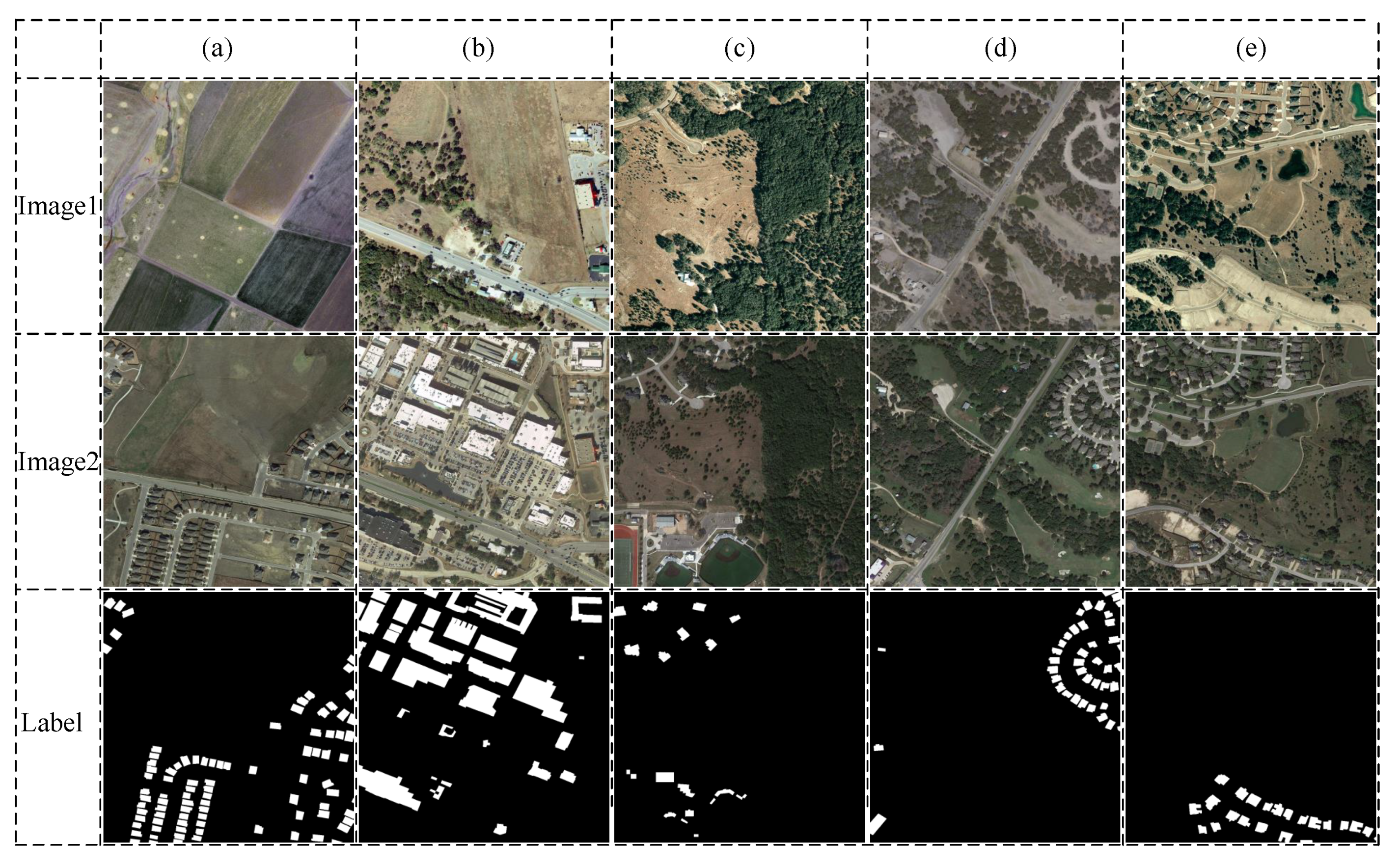
The 1024 × 1024 remote-sensing image is divided into 512 × 512 remote-sensing images due to computational resource constraints, as shown in Figure 10.

4. Experiment

To confirm the efficacy of our technique in achieving the change-detection objective, we conducted ablation experiments and comparison experiments. Our experiments were conducted on the TRS-CD and LEVIR-CD datasets, and our model was evaluated based on four metrics: ACC, RC, PR, and Miou.

4.1. Experimental Details

The deep learning framework used in the model code is PyTorch, and we conducted all experiments on a computer equipped with an RTX 3070 8GB graphics card. The learning rate is a crucial hyperparameter that significantly affects the training process and the final performance of the model. If the learning rate is consistently high, the model may fail to converge or diverge altogether. Conversely, if the learning rate is always low, the model may converge very slowly, and even if trained for an extended period, it may only reach a local optimal solution. In this paper, we employed an exponential decay mechanism for the learning rate, which started with a relatively high value in the early stages of training and gradually decreased over time. The decay rate and initial learning rate were carefully chosen through experimentation to achieve the optimal results. The formula for calculating how to change the learning rate is as follows:

$$\eta ={\eta }_0\times {\left(1-\frac{\mathrm{E}}{{\mathrm{E}}_{\mathrm{g}}}\right)}^{\mathrm{P}}$$

(13)

where $\eta$ stands for the adjusted learning rate, ${\eta }_0$ for the baseline learning rate, ${\mathrm{E}}_{\mathrm{g}}$ for the maximum number of iterations, and P a constant that regulates the learning-rate decay. Adam was selected as the optimization algorithm. Adam covers many optimization techniques and is a tool for running deep learning algorithms under python.

The loss function selects BCEWithLogitsLoss. Its specific calculation formula is as follows:

$$\mathrm{L}=\left\{l_1,\dots ,l_{\mathrm{N}}\right\},l_{\mathrm{n}}=-\left[y_{\mathrm{n}}·log\left(\mathrm{S}\left(x_{\mathrm{n}}\right)\right)+\left(1-y_{\mathrm{n}}\right)·log\left(1-\mathrm{S}\left(x_{\mathrm{n}}\right)\right)\right]$$

(14)

In the above formula, $\mathrm{S}\left(·\right)$ represents the sigmoid function. N is the number of batches. n is the number of labels in each batch. $x_{\mathrm{n}}$ is the predicted value, $y_{\mathrm{n}}$ is the label value, and $l_{\mathrm{n}}$ is the loss value of a single batch. L is the total loss. The BCEWithLogitsLoss function has a better robust performance when performing calculations.

We set the initial learning rate to 0.0015, the maximum number of iterations to 200, the momentum parameter P to 0.95, and the batch size to 6. Ablation experiments and comparison experiments were performed on the self-built TRS-CD dataset. The parameter settings of the two experiments were the same. We conducted experiments to evaluate the generalization performance of our model using the LEVIR-CD dataset, with a focus on testing the model’s ability to detect changes in unfamiliar environments. We set the maximum number of iterations to 100 and all other parameters are the same as the experiments on the self-built TRS-CD dataset.

4.2. Selection of Backbone

The first experiment was for picking out a better performing backbone network. The backbone networks chosen are mainly VGG [42] and ResNet [43]. The results of the experiment are shown in

Table 1. Comparative experiment of MHCNet under different backbone networks (bold numbers represent optimal results).

Backbone	ACC (%)	RC (%)	PR (%)	MIoU (%)
VGG16	93.96	63.83	74.63	76.70
VGG19	93.46	65.90	69.61	75.59
ResNet18	95.79	73.92	82.30	83.56
ResNet34	96.01	75.33	82.90	84.36

. The best results are shown in bold.

As shown in Table 1, ResNet achieved a higher accuracy than VGG. In addition, the residual structure of ResNet can effectively prevent performance degradation caused by deep network structures. Therefore, we chose ResNet34 as the backbone network for MHCNet.

4.3. Ablation Experiment of TRS-CD Dataset

We conducted ablation experiments on our self-built TRS-CD dataset to evaluate the impact of the auxiliary module on the performance of the entire network. Specifically, we varied the network architecture by adding an auxiliary module to assess the effect on the overall performance of the model. The experiment provided insight into their contribution to the final performance and parameters of the model.

Table 2. Ablation experiments of MHCNet (bold numbers represent optimal results).

Method	ACC (%)	RC (%)	PR (%)	MIoU (%)	Param (M)
Backbone	95.53	74.09	79.85	82.77	30.65
Backbone + CSAM	95.71	74.55	80.63	83.14	33.45
Backbone + CSAM + GSFM	95.80	74.59	81.71	83.58	36.25
Backbone + CSAM + GSFM + DBIFM	95.94	74.83	82.50	84.19	40.08
Backbone + CSAM + GSFM + DBIFM + SEM	96.01	75.33	82.90	84.36	40.43

shows the ablation results of MHCNet. Based on the backbone network, we add modules one by one to verify the effectiveness of each module. The training strategies of all models are the same. In this experiment, we mainly focus on the value of Miou.

The cross-scale feature-attention module (CSAM) proposed in the difference branch can optimize the ability of the difference branch to extract the difference semantic information and enable the two different scales of difference semantic information to guide each other to obtain the best possible difference semantic information. When this module is introduced, the value of Miou increases by $0.37\%$.

The global semantic filtering module (GSFM) acts on the global branch, which can extract and enhance the internal relationship between the two parts of the semantic information and then filter out the global semantic information of the changed region. After introducing this module, the value of Miou increases by $0.44\%$.

The double-branch information-fusion module (DBIFM) is a weighted fusion of the difference semantic information and the global semantic information focusing on the changing region. The value of Miou increases by $0.61\%$ after adding this module. The similarity-enhancement module (SEM) proposed in the similar branch tests the accuracy of the change region prediction from the invariant region and corrects the missed detection and false detection, improves the edge information, and increases the Miou value by $0.17\%$.

The four auxiliary modules of CSAM, GSFM, DBIFM, and SEM proposed by us increase the Miou by 0.37%, 0.44%, 0.60%, and 0.17%, respectively, and the final MHCNet increases the Miou by 1.59% compared with the basic network. Thus, we can conclude that for the change-detection task, each auxiliary module we propose can improve the ability of the network to extract features.

MHCNet has 40.43 M parameters. It is not difficult to see from Table 2 that MHCNet ’s backbone network has 30.65 M. This is because the backbone network uses two common parameters in ResNet34 that are used to extract features from two images respectively.

4.4. TRS-CD Dataset Comparison Test

In this section, we compared our proposed algorithm with existing change-detection algorithms. Given that semantic segmentation is a fundamental component of change-detection algorithms, we also included three traditional semantic-segmentation algorithms in our comparative experiments. This experiment provided a comprehensive evaluation of the performance of our model.To ensure a fair comparison, we initialized all parameters of the models randomly and learned them from scratch, even in cases where some networks had pre-trained parameters available. By training all models from scratch, we were able to assess their true performance and minimize the impact of any pre-existing biases or learned features.

Table 3. Comparative experiments on TRS-CD dataset (bold numbers represent optimal and suboptimal results).

Method	ACC (%)	RC (%)	PR (%)	MIoU (%)	Param (M)	Flops (GMac)
BiSeNet [44]	95.21	71.92	78.56	81.33	22.02	22.48
FCN8s [45]	92.85	66.06	66.84	74.49	18.65	80.68
UNet [46]	92.68	59.67	70.00	73.18	13.42	124.21
FC_DIFF [47]	91.12	39.27	74.83	65.87	11.35	19.29
FC_EF [47]	90.11	48.06	67.38	66.51	11.35	14.79
FC_CONC [47]	91.58	51.25	70.87	69.61	11.55	19.30
ChangNet [48]	94.18	62.78	75.62	76.88	23.52	42.73
TCDNet [49]	95.07	69.98	79.31	80.97	23.28	32.65
MFGANnet [50]	95.54	72.40	80.09	82.32	33.53	52.82
MHCNet (Ours)	96.01	75.33	82.90	84.36	40.43	59.07

presents the experimental outcomes.

Table 3 records the experimental results of MHCNet and other network models on the TRS-CD dataset. From the above data, the following four points can be obtained:

1.

The first three lines in the table are deep learning networks dedicated to semantic segmentation. The best-performing network is BiseNet, with a value of 81.5% for Miou, indicating that the change-detection task is a more complex binary semantic-segmentation task.

2.

Among other networks, FC_DIFF was specifically proposed for change detection in 2018 and achieved the lowest performance on the TRS-CD dataset with a Miou score of only 65.87%. In contrast, MFGANnet, proposed in 2022, achieved the highest performance with a Miou score of 82.32%. It can be seen that, over time, researchers have made breakthroughs in the field of change detection, and the proposed change-detection networks are becoming more and more effective.

3.

Our proposed MHCNet achieved a Miou score of 84.36% on the TRS-CD dataset, outperforming the second-best-performing MFGANnet by 2.04%. These results demonstrate that MHCNet is more effective than the other compared networks in the challenging task of change detection.

4.

MHCNet has a relatively large number of parameters compared to the other models. This is due to the dual-branch structure of MHCNet, which results in a large number of parameters in the backbone network, accounting for almost three-quarters of the total model parameters. Despite its relatively large number of parameters, the model complexity of MHCNet is at a medium level, making it a practical option for change-detection tasks.

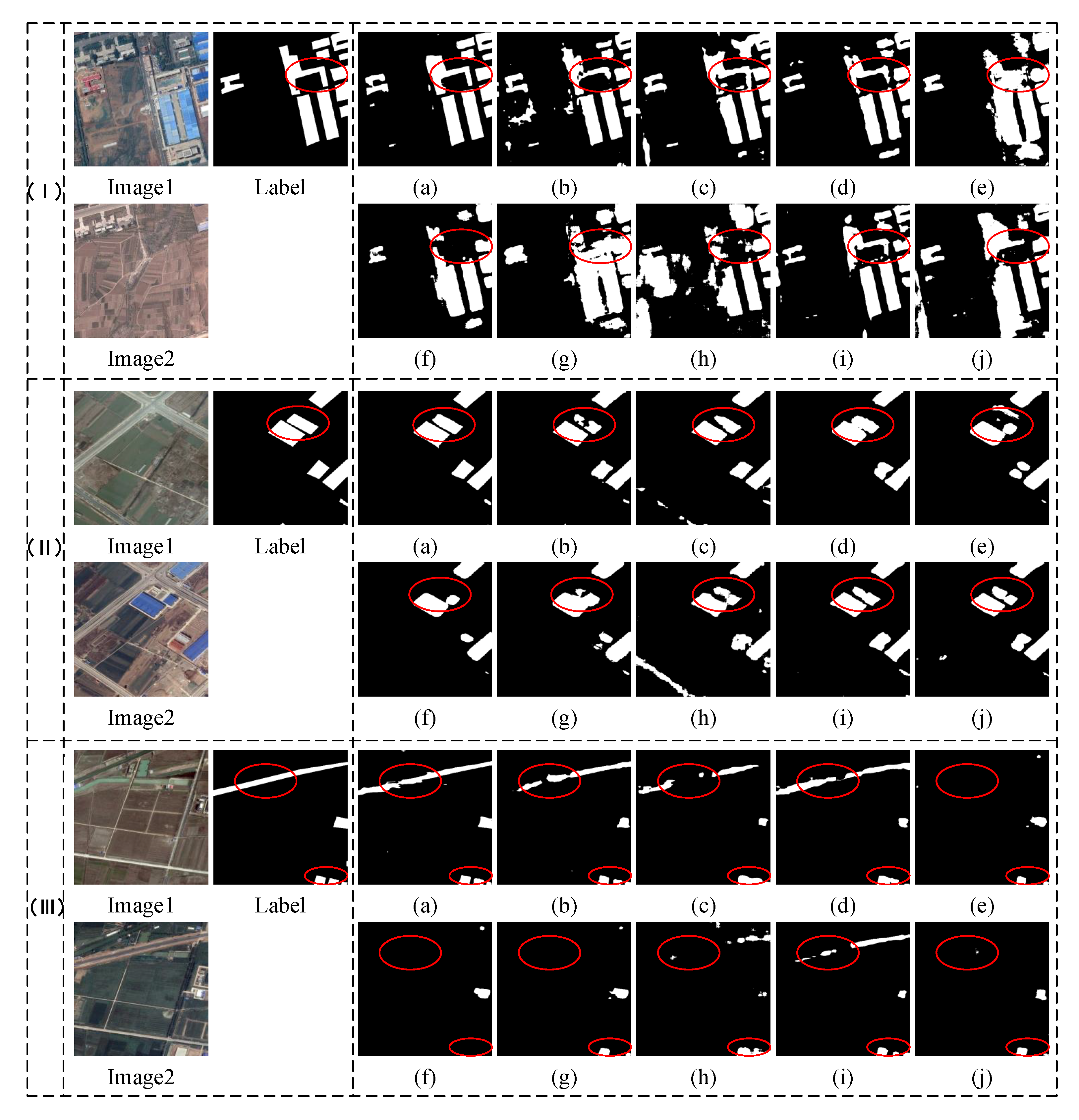
The test set of the self-built TRS-CD dataset contains 570 pairs of dual-temporal remote-sensing images. We selected three sets of predicted change maps for evaluation, corresponding to housing reform, land-use change, and water change, as shown in Figure 11. The first picture has a larger change area with relatively small sub-regions, which challenges the detection ability of the network. As shown by the red circle in the image, the other networks exhibit missed detections and their correctly detected areas have rough edges. In contrast, our network can effectively predict the change area with more delicate edges. In the second image, the results predicted by our model are basically consistent with the real labels and perform better than other networks. The change area of the third picture is a slender road. Some poorly performing networks cannot detect the change area, and the better-performing networks’ prediction results are also intermittent. Our network predicts a continuous change area. It can be seen from the performance in the prediction map that MHCNet performs best and has a higher performance than the other networks.

4.5. Comparative Experiments on the LEVIR-CD Dataset

In this section, we perform comparative experiments on the LEVIR-CD dataset to test the generalization and robustness of MHCNet. Due to the limitation of GPU physical memory, we simultaneously cut a 1024 × 1024 pixel two-time remote-sensing image into four 512 × 512 pixel images. Therefore, the number of images in the training set and the validation set of the LEVIR-CD dataset increased to 3600 and 480, respectively.

Table 4. Comparison experiments on the LEVIR-CD dataset (bold numbers represent optimal and suboptimal results).

Method	ACC (%)	RC (%)	PR (%)	MIoU (%)	Param (M)	Flops (GMac)
BiSeNet	98.04	80.49	78.74	83.36	22.02	22.48
FCN8s	98.39	79.08	83.33	84.68	18.65	80.68
UNet	98.62	81.32	84.69	86.25	13.42	124.21
FC_DIFF	98.46	78.84	85.72	85.26	11.35	19.29
FC_EF	97.94	80.26	78.07	82.86	11.35	14.79
FC_CONC	98.54	79.72	86.53	86.09	11.55	19.30
TCDNet	98.20	77.02	83.05	83.63	23.28	32.65
ChangNet	98.12	79.57	81.21	83.74	23.52	42.73
MFGANnet	98.30	78.49	84.70	84.73	33.53	52.82
MHCNet (Ours)	98.65	81.79	86.59	86.92	40.43	59.07

shows our experimental results. The first three networks in the table are behavior semantic segmentation networks, and the other networks are all change-detection private networks. The FC_EF network, which has a Miou index of just 82.86%, is the worst change-detection network on the LEVIR-CD dataset, as can be seen from the table, whereas the UNet network has a Miou index of 83.36%. Compared with the other networks, our MHCNet has the highest detection accuracy. The Miou index can reach 86.92%, which is 0.67% higher than that of UNet.

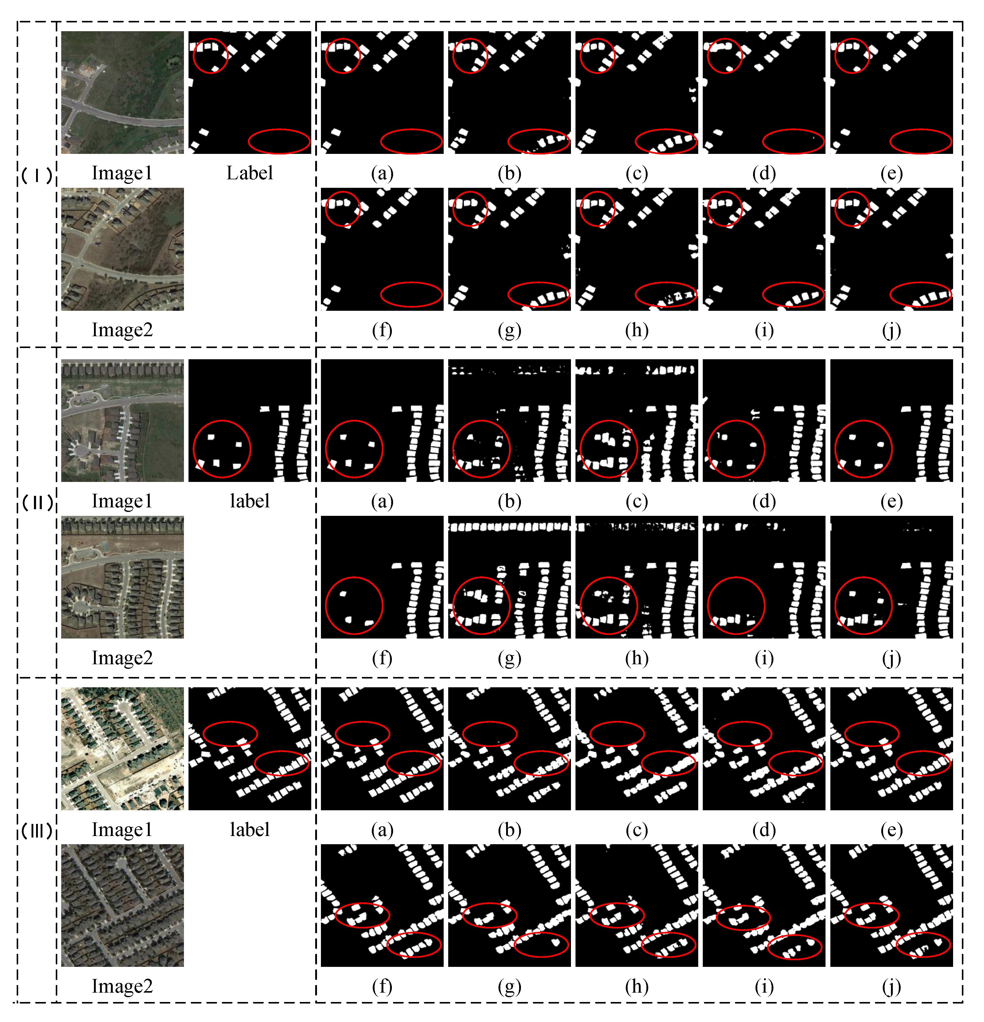
Figure 12 is a prediction diagram of three different situations we selected from the validation set. There are three situations depicted in these pictures: a transition from open space to some houses, a transition from some houses to a large number of houses, and changes that occur during the day and night. The first picture shows a transition from open space to a part of a house, resulting in a change area scattered throughout the entire picture, which makes it prone to missed detection. As seen from the prediction graph, only MHCNet perfectly predicts all regions, while the other networks have varying degrees of missed detection, multiple detection, and false detection. The second image depicts a series of small change areas side by side. Some networks with poor performance are unable to accurately detect the boundaries of the change area, resulting in incomplete predictions. However, the prediction results of the MHCNet network are the closest to the real label. In the third image, besides the numerous change areas, the image illumination significantly differs and there are many background interference factors. In this case, as shown in the red circle in the figure, apart from the prediction results of MHCNet, other networks exhibit shortcomings such as missed detection and insufficient detail in the shapes of their prediction results. The prediction results indicate that MHCNet has a high generalization ability and anti-interference ability.

4.6. Comparative Experiments on Cross-Dataset

Two sets of comparative experiments on the TRS-CD and LEVIR-CD datasets demonstrate that MHCNet exhibits an excellent feature-extraction ability and robust performance. Furthermore, we designed two additional experiments to further verify MHCNet’s robust performance:

1.

Train on the TRS-CD dataset and test on the LEVIR-CD dataset.

2.

Train on the LEVIR-CD dataset and test on the TRS-CD dataset.

In addition, these two sets of experiments also help to verify whether MHCNet has overfitting. For simplicity, we call these two datasets TRS-LEVIR and LEVIR-TRS.

Table 5. Comparative experiments on TRS-LEVIR dataset (bold numbers represent optimal and suboptimal results).

Method	ACC (%)	RC (%)	PR (%)	MIoU (%)	Param (M)	Flops (GMac)
BiSeNet	91.97	60.65	61.69	66.08	22.02	22.48
FCN8s	92.08	59.97	57.53	64.25	18.65	80.68
UNet	92.28	61.44	62.48	65.55	13.42	124.21
FC_DIFF	90.18	44.55	56.74	63.93	11.35	19.29
FC_EF	91.74	45.19	60.72	64.95	11.35	14.79
FC_CONC	90.46	44.85	59.11	63.86	11.55	19.30
TCDNet	90.83	63.62	63.32	66.31	23.28	32.65
ChangNet	91.07	54.07	56.68	62.80	23.52	42.73
MFGANnet	92.16	61.47	64.27	67.94	33.53	52.82
MHCNet (Ours)	92.44	63.30	65.12	68.71	40.43	59.07

and

Table 6. Comparative experiments on LEVIR-TRS dataset (bold numbers represent optimal and suboptimal results).

Method	ACC (%)	RC (%)	PR (%)	MIoU (%)	Param (M)	Flops (GMac)
BiSeNet	88.51	55.74	58.26	65.31	22.02	22.48
FCN8s	88.10	55.15	57.73	62.29	18.65	80.68
UNet	88.28	56.83	58.14	65.74	13.42	124.21
FC_DIFF	88.86	53.26	52.35	65.67	11.35	19.29
FC_EF	87.54	52.15	57.74	64.57	11.35	14.79
FC_CONC	88.61	54.36	51.49	65.55	11.55	19.30
TCDNet	88.48	55.57	55.84	66.24	23.28	32.65
ChangNet	88.23	56.09	54.70	64.10	23.52	42.73
MFGANnet	8.39	56.17	56.31	66.34	33.53	52.82
MHCNet (Ours)	88.90	57.12	58.02	66.78	40.43	59.07

show the indicators of all models on TRS-LEVIR and LEVIR-TRS, respectively.

The above two tables show that the indicators of all models on the two datasets are generally lower than the TRS-CD and LEVIR-CD datasets.This shows that the TRS-CD and LEVIR-CD datasets contain a large number of distinct samples. Models trained on one dataset struggle to accurately predict images from another dataset. Therefore, LEVIR can be selected as a suitable dataset for conducting generalization experiments to a certain extent. Second, MHCNet achieved the highest score on our primary evaluation metric, Miou. Additionally, MHCNet achieved basically the highest score on the other evaluation metrics, demonstrating that the model exhibits strong generalization and robustness.

5. Summary

First, we propose a multi-branch collaborative change-detection network based on Siamese structure (MHCNet). In this network, we introduce three branches to extract different semantic information, including a difference branch, global branch, and similar branch, to extract different semantic information, global semantic information, and similar semantic information of the change area. In addition, we propose four auxiliary modules, CSAM, GSFM, DBIFM, and SEM, to assist the three branches to extract semantic information. Finally, the extracted semantic information is supplemented into the recovery graph in the feature-decoding stage. From the perspective of the number of parameters and complexity of the model, NBCNet has the largest number of parameters, but it does not produce a large gap compared with MFGANnet. The complexity is at an upper moderate level, well below UNet and FCN8s. The specific process is as follows:

The CSAM module is proposed in the difference branch, which can optimize the ability of the difference branch to extract the difference semantic information and allow the difference semantic information of two different scales to guide each other to obtain the best possible difference semantic information. The GSFM module is proposed in the global branch, which can extract and enhance the internal relationship between the two parts of the semantic information and filter out the global semantic information of the change area. The DBIFM module combines the differential semantic information with the global semantic information that focuses on the changing region to help the model accurately determine the changing region. The SEM module is proposed in the similar branch. This module tests the accuracy of the change region prediction from the invariant region and corrects the missed detection and false detection to improve the edge information.

In the experiment, MHCNet can obtain higher evaluation indicators than other networks on the self-built TRS-CD dataset and the public LEVIR-CD dataset from a specific numerical point of view. The specific Miou indicators can reach 84.36% and 86.92%, respectively. MHCNet also received the best scores on the two datasets cross-acquired with TRS-CD and LEVIR-CD. The specific Miou indicators can reach 68.71% and 66.78%, respectively. From the effect of the comparison chart, MHCNet’s prediction chart is the closest to the real label. The summary is as follows:

1.

As can be seen from the comparison graph, MHCNet performs better at handling edge details, such as the shape of the river and adjacent houses, among others.

2.

Other networks have many missed detections, multiple detections, and false detections. MHCNet has few of these problems, and the prediction graph is closest to the real label.

3.

MFGANnet, BiseNet, and TCDNet ranked second, third, and fourth, respectively, on the TRS-CD dataset, but ranked fifth, sixth, and seventh on the LEVIR-CD dataset. In contrast, MCDNet achieves the best results on both the TRS-CD and LEVIR-CD datasets and exhibits superior robustness and generalization.

4.

MHCNet received the best score for every evaluation metric when tested on the cross-dataset. Despite having the largest number of parameters, MHCNet exhibits better generalization performance and does not exhibit significant signs of overfitting, indicating that the model performs quite well.

Currently, transformers are proven to be effective in the image domain. Some studies [51,52,53,54] have applied transformers to the field of remote-sensing image analysis. In the future, we should apply transformers to remote-sensing image change-detection tasks. In addition, the light weight of the model is also a research direction of scholars [55]. Due to the feature that a pair of images is required for the change-detection task, the number of parameters and the complexity of the model are often doubled. How to reduce the parameter amount and complexity of the model is crucial to future change-detection models.

References

1. He, C.; Wei, A.; Shi, P.; Zhang, Q.; Zhao, Y. Detecting land-use/land-cover change in rural–urban fringe areas using extended change-vector analysis. Int. J. Appl. Earth Obs. Geoinf. 2011, 13, 572–585. [Google Scholar] [CrossRef]
2. Sommer, S.; Hill, J.; Megier, J. The potential of remote sensing for monitoring rural land use changes and their effects on soil conditions. Agric. Ecosyst. Environ. 1998, 67, 197–209. [Google Scholar] [CrossRef]
3. Fichera, C.R.; Modica, G.; Pollino, M. Land Cover classification and change-detection analysis using multi-temporal remote sensed imagery and landscape metrics. Eur. J. Remote Sens. 2012, 45, 1–18. [Google Scholar] [CrossRef]
4. Eisavi, V.; Homayouni, S.; Karami, J. Integration of remotely sensed spatial and spectral information for change detection using FAHP. J. Fac. For. Istanb. Univ. 2016, 66, 524–538. [Google Scholar] [CrossRef]
5. Ma, Z.; Xia, M.; Lin, H.; Qian, M.; Zhang, Y. FENet: Feature enhancement network for land cover classification. Int. J. Remote Sens. 2023, 44, 1702–1725. [Google Scholar] [CrossRef]
6. Gillespie, T.W.; Chu, J.; Frankenberg, E.; Thomas, D. Assessment and prediction of natural hazards from satellite imagery. Prog. Phys. Geogr. 2007, 31, 459–470. [Google Scholar] [CrossRef]
7. Dong, L.; Shan, J. A comprehensive review of earthquake-induced building damage detection with remote sensing techniques. ISPRS J. Photogramm. Remote Sens. 2013, 84, 85–99. [Google Scholar] [CrossRef]
8. Weismiller, R.; Kristof, S.; Scholz, D.; Anuta, P.; Momin, S. Change detection in coastal zone environments. Photogramm. Eng. Remote Sens. 1977, 43, 1533–1539. [Google Scholar]
9. Ke, L.; Lin, Y.; Zeng, Z.; Zhang, L.; Meng, L. Adaptive change detection with significance test. IEEE Access 2018, 6, 27442–27450. [Google Scholar] [CrossRef]
10. Rignot, E.J.; Van Zyl, J.J. Change detection techniques for ERS-1 SAR data. IEEE Trans. Geosci. Remote Sens. 1993, 31, 896–906. [Google Scholar] [CrossRef]
11. Al Rawashdeh, S.B. Evaluation of the differencing pixel-by-pixel change detection method in mapping irrigated areas in dry zones. Int. J. Remote Sens. 2011, 32, 2173–2184. [Google Scholar] [CrossRef]
12. Comber, A.; Fisher, P.; Wadsworth, R. Assessment of a semantic statistical approach to detecting land cover change using inconsistent data sets. Photogramm. Eng. Remote Sens. 2004, 70, 931–938. [Google Scholar] [CrossRef]
13. Kesikoglu, M.H.; Atasever, U.; Ozkana, C. Unsupervised change detection in satellite images using fuzzy c-means clustering and principal component analysis. Int. Arch. Photogramm. Remote Sens. Spat. Inf. Sci. 2013, 7, W2. [Google Scholar] [CrossRef]
14. Hay, G.J. Visualizing 3-D Texture: A Three Dimensional Structural Approach to Model Forest Texture. Master’s Thesis, University of Calgary, Calgary, AB, Canada, 1995. [Google Scholar]
15. Shi, X.; Lu, L.; Yang, S.; Huang, G.; Zhao, Z. Object-oriented change detection based on weighted polarimetric scattering difference on polsar images. Int. Arch. Photogramm. Remote Sens. Spat. Inf. Sci. 2015, 40, 149–154. [Google Scholar] [CrossRef]
16. Leichtle, T.; Geiß, C.; Wurm, M.; Lakes, T.; Taubenböck, H. Unsupervised change detection in VHR remote sensing imagery—An object-based clustering approach in a dynamic urban environment. Int. J. Appl. Earth Obs. Geoinf. 2017, 54, 15–27. [Google Scholar] [CrossRef]
17. Desclée, B.; Bogaert, P.; Defourny, P. Forest change detection by statistical object-based method. Remote Sens. Environ. 2006, 102, 1–11. [Google Scholar] [CrossRef]
18. Shuai Zhang, L.W. STPGTN–A Multi-Branch Parameters Identification Method Considering Spatial Constraints and Transient Measurement Data. Comput. Model. Eng. Sci. 2023, 136, 2635–2654. [Google Scholar] [CrossRef]
19. Hu, K.; Ding, Y.; Jin, J.; Weng, L.; Xia, M. Skeleton Motion Recognition Based on Multi-Scale Deep Spatio-Temporal Features. Appl. Sci. 2022, 12, 1028. [Google Scholar] [CrossRef]
20. Hu, K.; Weng, C.; Zhang, Y.; Jin, J.; Xia, Q. An Overview of Underwater Vision Enhancement: From Traditional Methods to Recent Deep Learning. J. Mar. Sci. Eng. 2022, 10, 241. [Google Scholar] [CrossRef]
21. Wang, Z.; Xia, M.; Lu, M.; Pan, L.; Liu, J. Parameter Identification in Power Transmission Systems Based on Graph Convolution Network. IEEE Trans. Power Deliv. 2022, 37, 3155–3163. [Google Scholar] [CrossRef]
22. Ding, A.; Zhang, Q.; Zhou, X.; Dai, B. Automatic recognition of landslide based on CNN and texture change detection. In Proceedings of the 2016 31st Youth Academic Annual Conference of Chinese Association of Automation (YAC), Wuhan, China, 11–13 November 2016; IEEE: New York, NY, USA, 2016; pp. 444–448. [Google Scholar]
23. Wang, Q.; Yuan, Z.; Du, Q.; Li, X. GETNET: A general end-to-end 2-D CNN framework for hyperspectral image change detection. IEEE Trans. Geosci. Remote Sens. 2018, 57, 3–13. [Google Scholar] [CrossRef]
24. Zhan, Y.; Fu, K.; Yan, M.; Sun, X.; Wang, H.; Qiu, X. Change detection based on deep siamese convolutional network for optical aerial images. IEEE Geosci. Remote Sens. Lett. 2017, 14, 1845–1849. [Google Scholar] [CrossRef]
25. Zhang, W.; Lu, X. The spectral-spatial joint learning for change detection in multispectral imagery. Remote Sens. 2019, 11, 240. [Google Scholar] [CrossRef]
26. Liu, M.; Shi, Q.; Marinoni, A.; He, D.; Liu, X.; Zhang, L. Super-resolution-based change detection network with stacked attention module for images with different resolutions. IEEE Trans. Geosci. Remote Sens. 2021, 60, 1–18. [Google Scholar] [CrossRef]
27. Hu, K.; Li, M.; Xia, M.; Lin, H. Multi-Scale Feature Aggregation Network for Water Area Segmentation. Remote Sens. 2022, 14, 206. [Google Scholar] [CrossRef]
28. Miao, S.; Xia, M.; Qian, M.; Zhang, Y.; Liu, J.; Lin, H. Cloud/shadow segmentation based on multi-level feature enhanced network for remote sensing imagery. Int. J. Remote Sens. 2022, 43, 5940–5960. [Google Scholar] [CrossRef]
29. Chen, B.; Xia, M.; Qian, M.; Huang, J. MANet: A multi-level aggregation network for semantic segmentation of high-resolution remote sensing images. Int. J. Remote Sens. 2022, 43, 5874–5894. [Google Scholar] [CrossRef]
30. Chen, H.; Shi, Z. A spatial-temporal attention-based method and a new dataset for remote sensing image change detection. Remote Sens. 2020, 12, 1662. [Google Scholar] [CrossRef]
31. Chen, J.; Yuan, Z.; Peng, J.; Chen, L.; Huang, H.; Zhu, J.; Liu, Y.; Li, H. DASNet: Dual attentive fully convolutional Siamese networks for change detection in high-resolution satellite images. IEEE J. Sel. Top. Appl. Earth Obs. Remote Sens. 2020, 14, 1194–1206. [Google Scholar] [CrossRef]
32. Lu, C.; Xia, M.; Qian, M.; Chen, B. Dual-Branch Network for Cloud and Cloud Shadow Segmentation. IEEE Trans. Geosci. Remote Sens. 2022, 60, 1–12. [Google Scholar] [CrossRef]
33. Zhang, C.; Yue, P.; Tapete, D.; Jiang, L.; Shangguan, B.; Huang, L.; Liu, G. A deeply supervised image fusion network for change detection in high resolution bi-temporal remote sensing images. ISPRS J. Photogramm. Remote Sens. 2020, 166, 183–200. [Google Scholar] [CrossRef]
34. Peng, X.; Zhong, R.; Li, Z.; Li, Q. Optical remote sensing image change detection based on attention mechanism and image difference. IEEE Trans. Geosci. Remote Sens. 2020, 59, 7296–7307. [Google Scholar] [CrossRef]
35. Zhao, H.; Shi, J.; Qi, X.; Wang, X.; Jia, J. Pyramid scene parsing network. In Proceedings of the IEEE Conference on Computer Vision and Pattern Recognition, Honolulu, HI, USA, 21–26 July 2017; pp. 2881–2890. [Google Scholar]
36. Zhang, C.; Weng, L.; Ding, L.; Xia, M.; Lin, H. CRSNet: Cloud and Cloud Shadow Refinement Segmentation Networks for Remote Sensing Imagery. Remote Sens. 2023, 15, 1664. [Google Scholar] [CrossRef]
37. Qu, Y.; Xia, M.; Zhang, Y. Strip pooling channel spatial attention network for the segmentation of cloud and cloud shadow. Comput. Geosci. 2021, 157, 104940. [Google Scholar] [CrossRef]
38. Ma, Z.; Xia, M.; Weng, L.; Lin, H. Local Feature Search Network for Building and Water Segmentation of Remote Sensing Image. Sustainability 2023, 15, 3034. [Google Scholar] [CrossRef]
39. Yu, C.; Gao, C.; Wang, J.; Yu, G.; Shen, C.; Sang, N. Bisenet v2: Bilateral network with guided aggregation for real-time semantic segmentation. Int. J. Comput. Vis. 2021, 129, 3051–3068. [Google Scholar] [CrossRef]
40. Hu, K.; Weng, C.; Shen, C.; Wang, T.; Weng, L.; Xia, M. A multi-stage underwater image aesthetic enhancement algorithm based on a generative adversarial network. Eng. Appl. Artif. Intell. 2023, 123, 106196. [Google Scholar] [CrossRef]
41. Woo, S.; Park, J.; Lee, J.Y.; Kweon, I.S. Cbam: Convolutional block attention module. Proceedings of European Conference on Computer Vision (ECCV), Munich, Germany, 8–14 September 2018; pp. 3–19. [Google Scholar]
42. Simonyan, K.; Zisserman, A. Very deep convolutional networks for large-scale image recognition. arXiv 2014, arXiv:1409.1556. [Google Scholar]
43. He, K.; Zhang, X.; Ren, S.; Sun, J. Deep residual learning for image recognition. In Proceedings of the IEEE Conference on Computer Vision and Pattern Recognition, Las Vegas, NV, USA, 27–30 June 2016; pp. 770–778. [Google Scholar]
44. Yu, C.; Wang, J.; Peng, C.; Gao, C.; Yu, G.; Sang, N. Bisenet: Bilateral segmentation network for real-time semantic segmentation. In Proceedings of the European Conference on Computer Vision (ECCV), Munich, Germany, 8–14 September 2018; pp. 325–341. [Google Scholar]
45. Long, J.; Shelhamer, E.; Darrell, T. Fully convolutional networks for semantic segmentation. In Proceedings of the IEEE Conference on Computer Vision and Pattern Recognition, Boston, MA, USA, 7–12 June 2015; pp. 3431–3440. [Google Scholar]
46. Ronneberger, O.; Fischer, P.; Brox, T. U-net: Convolutional networks for biomedical image segmentation. In Proceedings of the International Conference on Medical Image Computing and Computer-Assisted Intervention, Munich, Germany, 5–9 October 2015; Springer: Cham, Switzerland, 2015; pp. 234–241. [Google Scholar]
47. Daudt, R.C.; Le Saux, B.; Boulch, A. Fully convolutional siamese networks for change detection. In Proceedings of the 2018 25th IEEE International Conference on Image Processing (ICIP), Athens, Greece, 7–10 October 2018; IEEE: New York, NY, USA, 2018; pp. 4063–4067. [Google Scholar]
48. Varghese, A.; Gubbi, J.; Ramaswamy, A.; Balamuralidhar, P. ChangeNet: A deep learning architecture for visual change detection. In Proceedings of the European Conference on Computer Vision (ECCV) Workshops, Munich, Germany, 8–14 September 2018. [Google Scholar]
49. Liu, Y.; Pang, C.; Zhan, Z.; Zhang, X.; Yang, X. Building change detection for remote sensing images using a dual-task constrained deep siamese convolutional network model. IEEE Geosci. Remote Sens. Lett. 2020, 18, 811–815. [Google Scholar] [CrossRef]
50. Chu, S.; Li, P.; Xia, M. MFGAN: Multi feature guided aggregation network for remote sensing image. Neural Comput. Appl. 2022, 34, 10157–10173. [Google Scholar] [CrossRef]
51. Song, L.; Xia, M.; Weng, L.; Lin, H.; Qian, M.; Chen, B. Axial Cross Attention Meets CNN: Bibranch Fusion Network for Change Detection. IEEE J. Sel. Top. Appl. Earth Obs. Remote Sens. 2023, 16, 32–43. [Google Scholar] [CrossRef]
52. Lu, C.; Xia, M.; Lin, H. Multi-scale strip pooling feature aggregation network for cloud and cloud shadow segmentation. Neural Comput. Appl. 2022, 34, 6149–6162. [Google Scholar] [CrossRef]
53. Chen, J.; Xia, M.; Wang, D.; Lin, H. Double Branch Parallel Network for Segmentation of Buildings and Waters in Remote Sensing Images. Remote Sens. 2023, 15, 1536. [Google Scholar] [CrossRef]
54. Hu, K.; Zhang, E.; Xia, M.; Weng, L.; Lin, H. MCANet: A Multi-Branch Network for Cloud/Snow Segmentation in High-Resolution Remote Sensing Images. Remote Sens. 2023, 15, 1055. [Google Scholar] [CrossRef]
55. Gao, J.; Weng, L.; Xia, M.; Lin, H. MLNet: Multichannel feature fusion lozenge network for land segmentation. J. Appl. Remote Sens. 2022, 16, 1–19. [Google Scholar] [CrossRef]
Figure 1. The network framework of MHCNet. Four auxiliary modules are proposed in MHCNet, which are the cross-scale feature-attention module (CSAM), global semantic filtering module (GSFM), double-branch information-fusion module (DBIFM), and similarity-enhancement module (SEM).
Remotesensing 15 02237 g001
Figure 2. Structure of cross-scale feature-attention module.
Remotesensing 15 02237 g002
Figure 3. Structure of global semantic filtering module.
Remotesensing 15 02237 g003
Figure 4. Structure of double-branch information-fusion module.
Remotesensing 15 02237 g004
Figure 5. Structure of similarity-enhancement module.
Remotesensing 15 02237 g005
Figure 6. Improved pyramid pooling module structure.
Remotesensing 15 02237 g006
Figure 7. Heatmap where (a) represents the heat map of the backbone network + SEM, (b) represents the heat map after adding CSAM to the basis of (a), (c) represents the heat map after adding GSFM to the basis of (b), (d) represents the heat map after adding DBIFM to (c), and (e) is a real label diagram. As illustrated in the figure, the model’s attention to the changing areas gradually increases as the modules are continuously stacked. This observation indicates the effectiveness of each of our modules in improving the model’s ability to represent features.
Remotesensing 15 02237 g007
Figure 8. BTRS-CD dataset. Each column represents a pair of two-time remote -ensing images, image1 and image2 are real remote-sensing images, and label is a label (white is the change region, black is the invariant region).Where, (a) represents the no-change area, (b) represents the construction of factories, (c) represents the transformation of roads into fields, (d) represents the transformation of factories into vacant land, and (e) represents the changes within the building complex.
Remotesensing 15 02237 g008
Figure 9. The proportion distribution map of the change area of the BTRS-CD dataset. The percent of the changing area is plotted along the horizontal axis, and the sample size is plotted along the vertical axis.
Remotesensing 15 02237 g009
Figure 10. LEVIR dataset diagram. Each column represents a pair of two-time remote-sensing images, image1 and image2 are real remote-sensing images, and label is a label (white is the change region, black is the invariant region). Where, (a) represents the conversion of good land to buildings, (b) represents the conversion of forests to buildings (concentrated change areas), (c) represents conversion of forests to buildings (scattered change areas), (d) represents conversion of forests to buildings (uneven distribution of change areas), and (e) represents building houses on open land.
Remotesensing 15 02237 g010
Figure 11. Prediction graphs of different algorithms on TRS-CD dataset. A comparison of three pairs of dual-time remote-sensing images is presented in (I–III). Image1 and Image2 represent bi-temporal Google Earth images; label means label; (a) represents our MHCNet prediction graph; (bj) represent the prediction maps for MFGANnet, BiSiNet, ChangNet, FC_CONC, FC_DIFF, FC_EF, FCN8s, TCDnet, and UNet, respectively.
Remotesensing 15 02237 g011
Figure 12. Prediction of different algorithms on the LEVIR-CD dataset. A comparison of three pairs of dual-time remote-sensing images is presented in (I–III). Image1 and Image2 represent bi-temporal Google Earth images; label means label; (a) represents our MHCNet prediction graph; (bj) represent the prediction maps for MFGANnet, BiSiNet, ChangNet, FC_CONC, FC_DIFF, FC_EF, FCN8s, TCDnet, and UNet, respectively.
Remotesensing 15 02237 g012