MFNet: Mutual Feature-Aware Networks for Remote Sensing Change Detection

Abstract

Remote sensing change detection involves detecting pixels that have changed from a bi-temporal image of the same location. Current mainstream change detection models use encoder-decoder structures as well as Siamese networks. However, there are still some challenges with this: (1) Existing change feature fusion approaches do not take into account the symmetry of change features, which leads to information loss; (2) The encoder is independent of the change detection task, and feature extraction is performed separately for dual-time images, which leads to underutilization of the encoder parameters; (3) There are problems of unbalanced positive and negative samples and bad edge region detection. To solve the above problems, a mutual feature-aware network (MFNet) is proposed in this paper. Three modules are proposed for the purpose: (1) A symmetric change feature fusion module (SCFM), which uses double-branch feature selection without losing feature information and focuses explicitly on focal spatial regions based on cosine similarity to introduce strong a priori information; (2) A mutual feature-aware module (MFAM), which introduces change features in advance at the encoder stage and uses a cross-type attention mechanism for long-range dependence modeling; (3) A loss function for edge regions. After detailed experiments, the F1 scores of MFNet on SYSU-CD and LEVIR-CD were 83.11% and 91.52%, respectively, outperforming several advanced algorithms, demonstrating the effectiveness of the proposed method.

1. Introduction

In recent years, remote sensing technology has advanced rapidly, resulting in significant improvements in the imaging capability and quality of remote sensing satellites. Optical remote sensing images now offer a resolution that exceeds 0.1 GSD (ground sampling interval, which indicates the ground distance represented by each pixel). This enhanced resolution facilitates the clear and precise identification of surface objects using remote sensing images. As a result, remote sensing images have become a widely used tool for identifying and analyzing ground objects; change detection is an important application of this technique.

Remote sensing change detection refers to the analysis of images from the same geographical area captured at different times to identify changes in features of interest within a specific time range [1]. It can be applied to a variety of scenarios, such as arable land changes, building changes, lake and river changes, road network changes, etc. [2,3,4]. Remote sensing change detection technology is important for national land regulation, modern urban planning, natural disaster assessment [5], and military facility reconnaissance. Therefore, studying change detection algorithms with higher accuracy is of great theoretical significance and application value.

Numerous studies have explored the problem of change detection in remote sensing images. The accuracy of traditional methods is relatively low due to the effects of atmospheric conditions and seasonal variations, the nature of satellite sensors, and solar elevation.

Recently, deep learning methods have gained widespread use in remote sensing change detection. These techniques are capable of automatically extracting complex, hierarchical, and nonlinear features from raw data, overcoming the limitations of traditional change detection methods and exhibiting outstanding performance. Based on the deep feature extraction process of dual-temporal images, deep-learning-based change detection frameworks can be categorized into three types: single-stream, double-stream, and multi-model integrated [6]. The double-stream Siamese networks have received more attention due to their simpler structure and stronger performance. In double-stream Siamese networks, the deep models used to extract features can be classified as convolutional neural-network-based models [7,8], recurrent neural-network-based models [9,10,11], Transformer-based models [12,13], adversarial generative network-based models [14], etc. [15].

Convolutional neural networks can preserve neighborhood connections and local features and can process images of large size due to their structure of shared convolutional kernels. The FC-EF [7] and FC-diff [7] algorithms were the pioneers in utilizing a fully convolutional Siamese network architecture with skip connections. These methods were the first to employ end-to-end training and fully convolutional neural networks, improving the network’s accuracy and inference speed without increasing the training time. Subsequently, researchers [8,12,16,17,18,19,20,21,22] extensively employed the Siamese network encoder and UNet decoder architectures as a base model for change detection. SNUNet-CD [8] increases the flow path of multi-scale features in the decoder part, reducing the loss of localization information of shallow neural network features. ECAM [23] is designed to refine the most representative output at different feature scales.

Recurrent neural networks are very effective in capturing sequence relationships, and in change detection; they can effectively establish change relationships between dual-temporal images. REFEREE [9] is based on an improved long short-term memory (LSTM) model to acquire and record change information of long-term serial remote sensing data, using core storage units to learn change rules from information about binary changes or multi-class changes. In addition, there are algorithms that combine CNN and RNN to implement change detection. SiamCRNN [10] uses a deep Siamese convolutional neural network to accomplish feature extraction and uses spatial-spectral features extracted from stacked long- and short-term memory units to map to a new latent feature space and to mine change information between them. In FCD-R2U-net [11], in order to reduce the possible loss of topological information in changing regions, the classical R2U-Net structure is improved using a pair of R2CUs instead of a single R2CU in each convolutional layer of the encoder and decoder paths to make the model focus on certain detailed changing forest objects.

Transformer [24] can extract contextually relevant feature representations through a multi-head self-attention mechanism and has been widely used in remote sensing image processing in recent years. BIT [12] uses an effective transformer-based [24] change detection method for remote sensing images. This method expresses the input image as visual words and models the context in a compact token-based space-time, facilitating the identification of change features of interest, while excluding irrelevant non-change features. The Changeformer [13] algorithm is the first pure transformer-based change detection model. It leverages the MIT [25] backbone network, which excels in semantic segmentation models, for the change detection task, integrating a hierarchically structured transformer encoder with a multi-layer perceptual decoder to effectively extract the desired multi-scale long-range relations.

However, these algorithms operate within a Siamese network architecture where the encoder part is not optimized for the change detection task. The extraction of change features is performed only at the decoder, resulting in underutilization of the encoder parameters.

Furthermore, extraction of change features is crucial for change detection tasks. Some studies [1,19,20,26,27] have sought to improve the performance of change detection by enhancing the fusion of multi-scale features. The STANet [1] algorithm incorporates a change detection self-attention module after the encoder network, allowing for the computation of spatiotemporal relationships between any two pixels in the change detection input image. Additionally, it uses different scales of self-attention to account for the scale diversity of the building target attention mechanism, resulting in more effective change features. The FCCDN [26] algorithm introduces a feature fusion module, DFM, based on dense connectivity that is both simple and effective. The module includes difference and summation branches, where the summation branch enhances edge information, and the difference branch generates regions of variation. Each branch is constructed from two streams of shared weights that are densely connected, reducing feature misalignment. The DSANet [19] algorithm uses a remote sensing change detection method based on deep metric learning. It uses a dual attention module to improve feature discrimination and more robustly distinguish changes. SCFNet [27] introduces a structure of self-attention and convolutional layer fusion in the deepest layer of the encoder to better capture the semantic and positional mapping of different buildings in the study area, providing more informative features for subsequent feature fusion.

However, to ensure symmetry between the front and back temporal phases in the change detection task, prediction results should be the same regardless of whether the image of temporal phase one or the image of temporal phase two is input first. Some existing change feature fusion algorithms do not consider this symmetry, while others use a complex attention mechanism.

In this paper, we propose a solution to the problem of symmetry in change features by introducing a symmetric change feature fusion module (SCFM). The SCFM uses a two-branch feature selection approach, which preserves feature information, while incorporating strong prior knowledge, and a spatial feature attention mechanism based on cosine similarity. To fully utilize the encoder parameters and address the issue of delayed change feature extraction, we propose the interaction feature-aware module (MFAM) in the encoder stage. The MFAM incorporates change features into the encoder stage and uses a cross-type attention mechanism to model long-range dependencies. We also address sample imbalance and poor edge detection in change detection by introducing the Dice loss function for edge region detection.

The main contributions of this paper are summarized as follows:

• A symmetric change feature fusion module (SCFM) is proposed, which uses parallel feature differencing and feature summation to maintain the symmetry of the results, while employing feature channel selection attention and explicit spatial attention based on cosine similarity to enhance the model’s extraction of change features.
• A mutual feature-aware module (MFAM) is proposed to introduce change features in the deep stage of encoders based on the Siamese network architecture, which can make fuller use of the powerful parametric number of encoders and feature extraction for the focused regions that need attention compared to previous work.
• We propose a new loss function (EL) for improving the effect of edge region change detection.
• Based on the above three structures, we propose a mutual feature-aware network (MFNet) for remote sensing image change detection. Moreover, we conducted extensive experiments on public datasets SYSU-CD and LEVIR-CD and achieved advanced performance with F1 scores of 83.11% and 91.52%, respectively.

This paper is organized as follows: In Section 2, we describe the overall framework and detailed structure of the algorithm proposed in this paper. In Section 3, the evaluation results on public datasets are shown and compared with current state-of-the-art algorithms. In Section 4, a detailed ablation experiment with visualization is discussed. The Section 5 concludes the full paper.

2. Methods

2.1. Overview

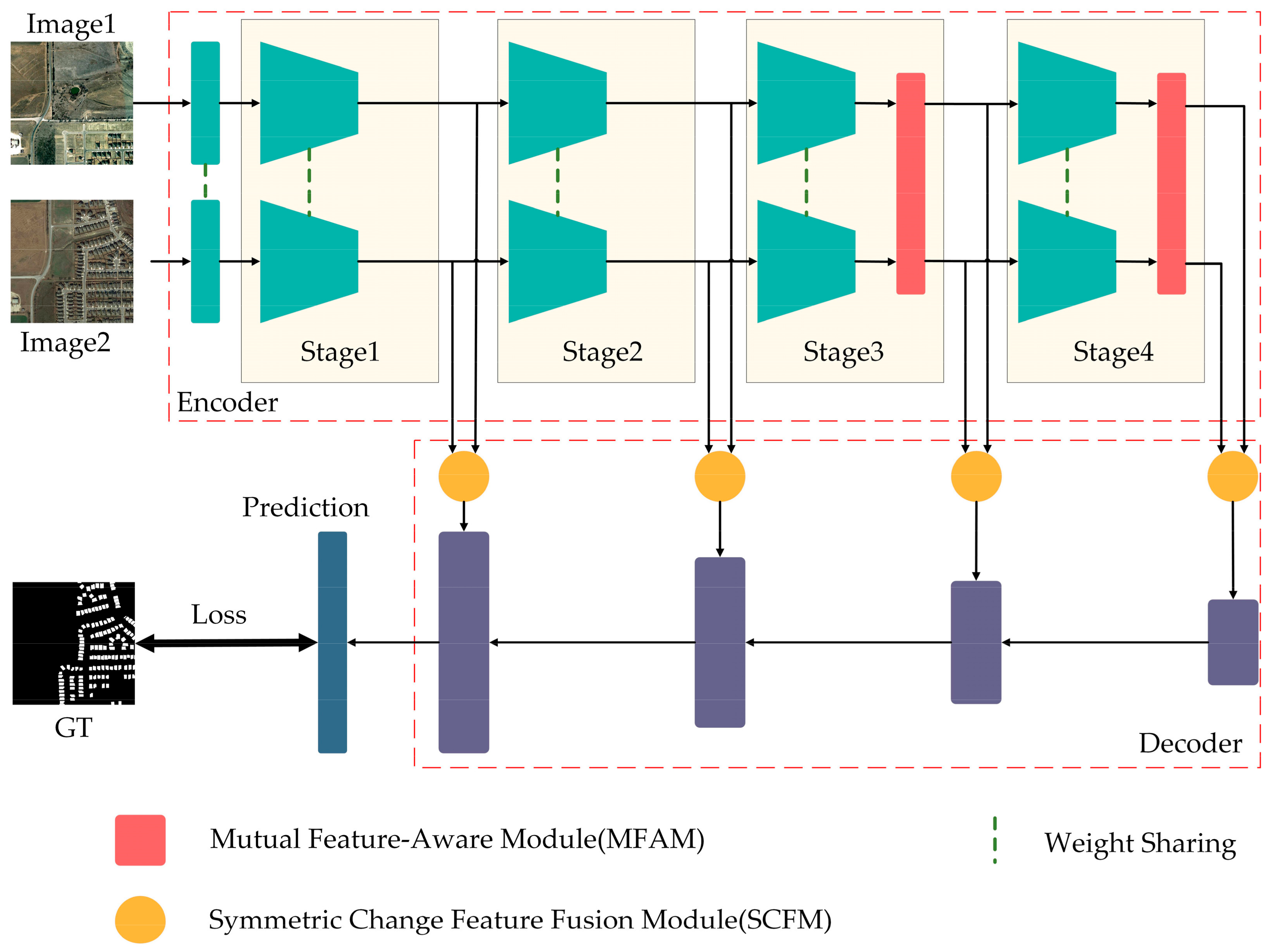
The overall structure of the mutual feature-aware network (MFNet) constructed in this paper is shown in Figure 1. An encoder-decoder structure is used, with the encoder using a twin shared weight network to extract features from dual-temporal images and the decoder using a feature pyramid fusion network to fuse multi-scale features.

The inputs of the model are two pre-aligned images at different times, which are extracted by a Siamese encoder to obtain four multi-scale features, respectively.

In the encoder, since there is more high-level semantic information in the deep network, the mutual feature-aware module MFAM proposed in this paper is used after stage 3 and stage 4 to perceive the change features in advance in the encoding stage and enhance the feature extraction capability of the model.

In the decoder, four scales of features from the encoder are input, and, at each scale, the change features are obtained by fusing the features from the dual-temporal features through the symmetric change feature fusion module SCFM proposed in this paper. Finally, the change features from multiple scales are up-sampled and fused using a feature pyramid fusion network [28].

2.2. Symmetric Change Feature Fusion Module

The symmetric change feature fusion module (SCFM) is used in the decoder. Its input is a pair of features [$F_{Ai},F_{B_i}$] from different times, which are fused to output the change feature $F_{Ci}$, where i indicates different stages of the encoder; the symmetric structure can ensure that $F_{Ci}$ is independent of the input sequence of [$F_{Ai},F_{B_i}$]. The specific structure is shown in Figure 2a.

It consists of three main steps.

1. Parallel branching is used to sum, as well as find the difference for, [$F_{Ai},F_{B_i}$]. The absolute value operation is used to maintain the symmetry after the difference. The feature difference can provide good a priori knowledge of the changes and highlight the features that have changed, but there is a large amount of feature loss when making the difference, and the summation branch can compensate for this information loss while maintaining the symmetry of the structure. This step can be formulated as follows:

$$F_{add}=F_{Ai}+F_{Bi}$$

(1)

$$F_{diff}=abs\left(F_{Ai}-F_{Bi}\right)$$

(2)

2. Feature selection is performed at the feature channel level using the feature selection module (FSM) for the results of the above parallel branching. The specific structure of the FSM is shown in Figure 2b, which is similar to the squeeze and excitation module (SE [29]), where the spatial dimension of the features is first compressed using average-pooling, the 1 × 1 convolution is used for feature mapping, and then the sigmoid is used for feature activation to obtain the importance of different feature channels. This is weighted on the original features and combined with the original features through the residual connection [30]. The feature selection module enables selection of the more important feature channels in this branch. This step can be formulated as follows:

$$F_{branch1},F_{branch2}=\mathrm{FSM}\left(F_{add}\right),\mathrm{FSM}\left(F_{diff}\right)$$

(3)

3. The feature selection results of the dual branch are concatenated in the channel dimension. Then the features are enhanced in the spatial dimension by the explicit dissimilarity weighting module (DWM). The specific structure of the DWM is shown in Figure 2c. First, the cosine dissimilarity is calculated in the channel dimension for the input features [$F_{Ai},F_{B_i}$], which is represented as follows:

$$\begin{gathered} D{S}_{m,n}=\frac{1-CosSimilarit{y}_{AB}}{2} \\ =\left(1-\frac{F_{A,m,n}\cdot F_{B,m,n}}{\left|F_{A,m,n}\right|*\left|F_{B,m,n}\right|}\right)/2 \end{gathered}$$

(4)

where m and n denote the spatial coordinates of the feature points, $D{S}_{m,n}$∈[0, 1]—the closer its value is to 1, the smaller the similarity. This position is more likely to be changed; thus, the feature weights here need to be increased. After obtaining the DS, it is weighted to the original input features and combined with the input features through a residual connection. Finally, the features are extracted by a conv-bn-relu module. The dissimilarity weighting module allows for enhanced extraction of change features in the spatial dimension, and the calculation of dissimilarity introduces a certain amount of a priori knowledge. This step can be formulated as follows:

$$F_{cat}=Concat\left(F_{branch1},F_{branch2}\right)$$

(5)

$$F_c=DWM\left(F_{cat}\right)$$

(6)

2.3. Mutual Feature-Aware Module

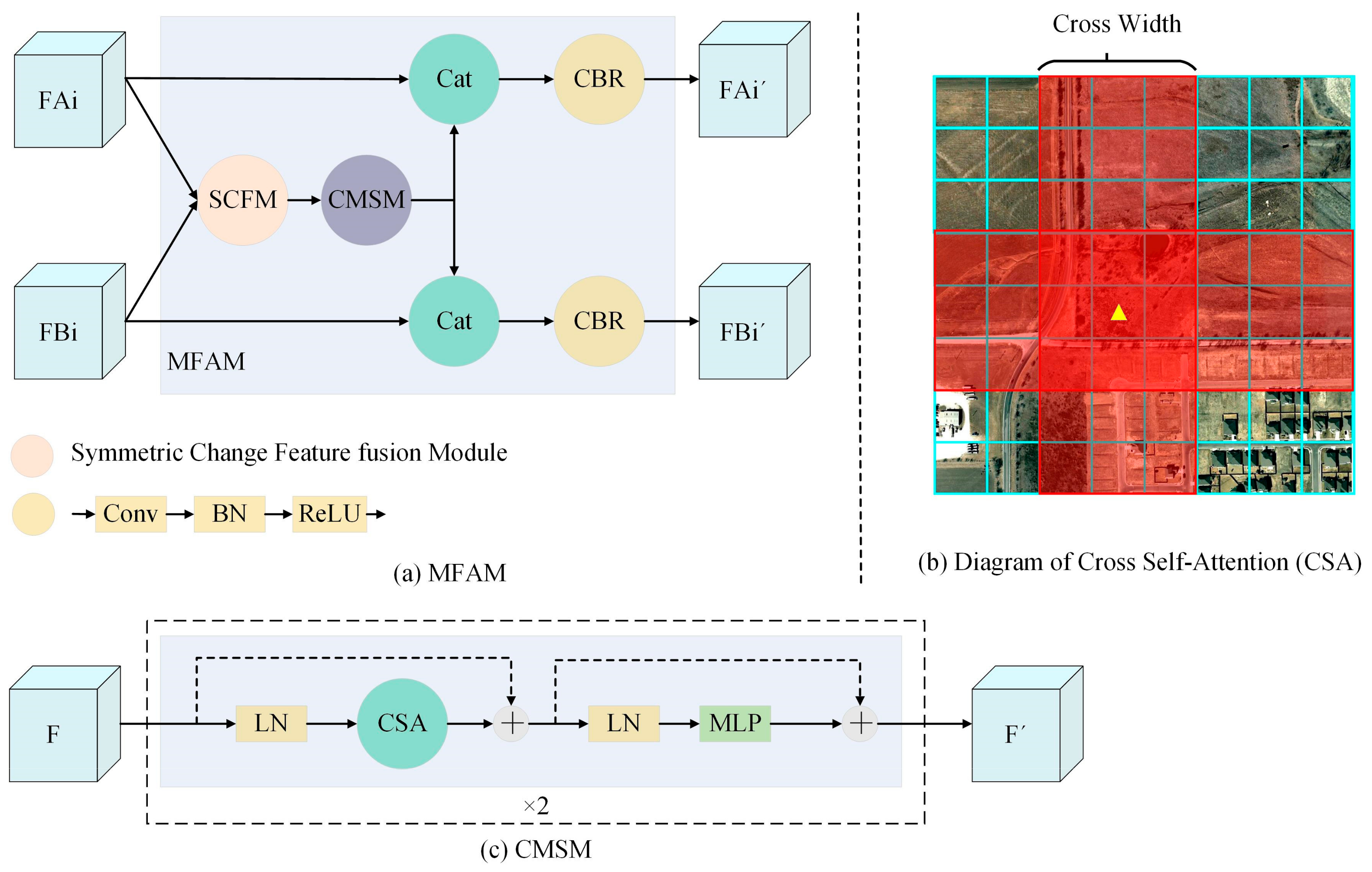
The mutual feature-aware module (MFAM) is used in the encoder. The module is only used after stage 3 and stage 4 because the semantic information of the shallow network features of the encoder is low and the change features cannot be extracted effectively. The inputs of MFAM are the features [$F_{Ai},F_{B_i}$] from the previous stage of the encoder, and the outputs are [${F_{Ai}}^{\prime },{F_{B_i}}^{\prime }$] after the mutual feature awareness; perceiving the change features in advance in the encoder can guide the model to focus on the focal regions. The specific structure of this module is shown in Figure 3a.

It consists of three main steps:

1. The symmetric change feature fusion module introduced in the previous subsection is used; the bi-temporal change features are extracted based on the bi-temporal input features.

2. The cross multi-headed self-attention module [31] (CMSM) is used to model the interaction features for long-distance relationships. The specific structure of CMSM is shown in Figure 3c. The input features are normalized over all channels by the LayerNorm layer and then pass through the cross self-attention layer (CSA), as shown in Figure 3b. The spatial dimension of the whole feature map is H × W. Each small blue square represents a spatial feature point; the yellow triangle indicates the point of the currently calculated feature, whose spatial location is denoted as ($m,n$). The attention of the current yellow triangle point is calculated with the points in the red region, as shown in Figure 3b, where the width of the cross is symmetrically distributed on both sides of the current point. The calculation is as follows:

$$\begin{gathered} F_{m,n}=softmax\left(\frac{Q_{m,n}*K_{i,j}^T}{\sqrt{d}}\right)*V_{i,j} \\ \left\{i\in \left[m-\frac{C_W}{2},m+\frac{C_W}{2}\right],j\in \left[0,w-1\right]\right\}\cup \left\{i\in \left[0,h-1\right],j\in \left[n-\frac{C_W}{2},n+\frac{C_W}{2}\right]\right\} \end{gathered}$$

(7)

where $C_W$ indicates the cross width, $w$ and $h$ indicate the width and height of the feature, $QKV$ is obtained by mapping the original features to different linear spaces, and $d$ indicates the dimension of $Q$.

Computing the features of a point requires computing the self-attention $C_W\times H+C_W\times W-C_W{}^2$ times, which are much smaller compared to the $H\times W$ times of global self-attention [32]. After calculating the cross self-attention once, the current point still cannot perceive the features in the blue squares in the figure, but, after one stacking, i.e., using two CMSM modules, the current point has directly or indirectly calculated the self-attention features with all other points, so two CMSM structures in series are used here. As the encoder network deepens, the spatial dimension of the features is gradually downsampled. In order to directly obtain a larger range of feature attention, we adopt the strategy of gradually increasing $C_W$. Specifically, the $C_W$ after stage 3 and stage 4 of the encoder is 3 and 5, respectively.

3. The mutual features acquired by the CMSM module are concatenated to the input features [$F_{Ai},F_{B_i}$], and the mutual features are perceived by a convolution–BN–activation combination.

2.4. Edge Loss

The online hard example mining (OHEM) and edge Dice loss (EDL) modules solve the problems of sample imbalance and difficult edge detection in remote sensing change detection by improving the optimization objectives of the model.

Change detection is a pixel-level binary classification problem, commonly using binary cross-entropy loss as the optimization objective. The online hard example mining loss is determined by sorting the pixel-by-pixel bce loss, and then taking the largest TopK pixel loss, and calculating their mean value; in this paper K has a value of 50,000. In this way a large number of simple samples are filtered out as a way to solve the problem of imbalance between difficult and easy samples. The calculation is as follows:

$$Los{s}_{BCE}=y_{\dot{i}}\cdot {\log }_P\left(y_i\right)+\left(1-y_i\right)\cdot \log \left(1-y_i\right)$$

(8)

$$Los{s}_{OHEM}=\frac{\sum TopK\left(Los{s}_{BCE}\right)}{K}$$

(9)

Dice loss is a commonly used loss function in semantic segmentation, which can measure the similarity of two sets from a global perspective. Even when there are only a very small number of positive samples in an image, Dice loss can still work. Using this loss can solve the problem of extreme imbalance between positive and negative samples, which is calculated as in Equation (10)

$$Los{s}_{Dice}=1-\frac{2\left|X\cap Y\right|}{\left|X\right|+\left|Y\right|}$$

(10)

In this paper, we propose edge Dice to make the model focus on more difficult pixel classification at the edge of the object, as shown in Figure 4. The left figure is the label of change detection, first extracting its edge, and then extending w pixels inward and outward, as shown in the right figure. In this paper, w is taken as 20 pixels, the red region is the positive sample region, the yellow region is the negative sample region, and Dice loss is calculated only in these two regions to obtain $Los{s}_{Edge}$.

Total losses are as follows:

$$Los{s}_{Total}=Los{s}_{OHEM}+Los{s}_{Dice}+Los{s}_{Edge}$$

(11)

3. Results

3.1. Remote Sensing Change Detection Dataset

Remote sensing change detection datasets can be broadly categorized into two types: generic change detection and domain-specific change detection. The former focuses on detecting multiple change types at the same time, treating them as the same class. Examples of such datasets include CDD [33], SYSU-CD [18], SECOND [34], etc. The latter type, on the other hand, is specific to a particular change type, such as building change detection. Datasets falling under this category include LEVIR-CD [1], WHU-CD [35], S2Looking [36], etc. In this paper, we conduct experiments using one dataset from each of these two categories, namely SYSU-CD and LEVIR-CD.

3.1.1. SYSU-CD

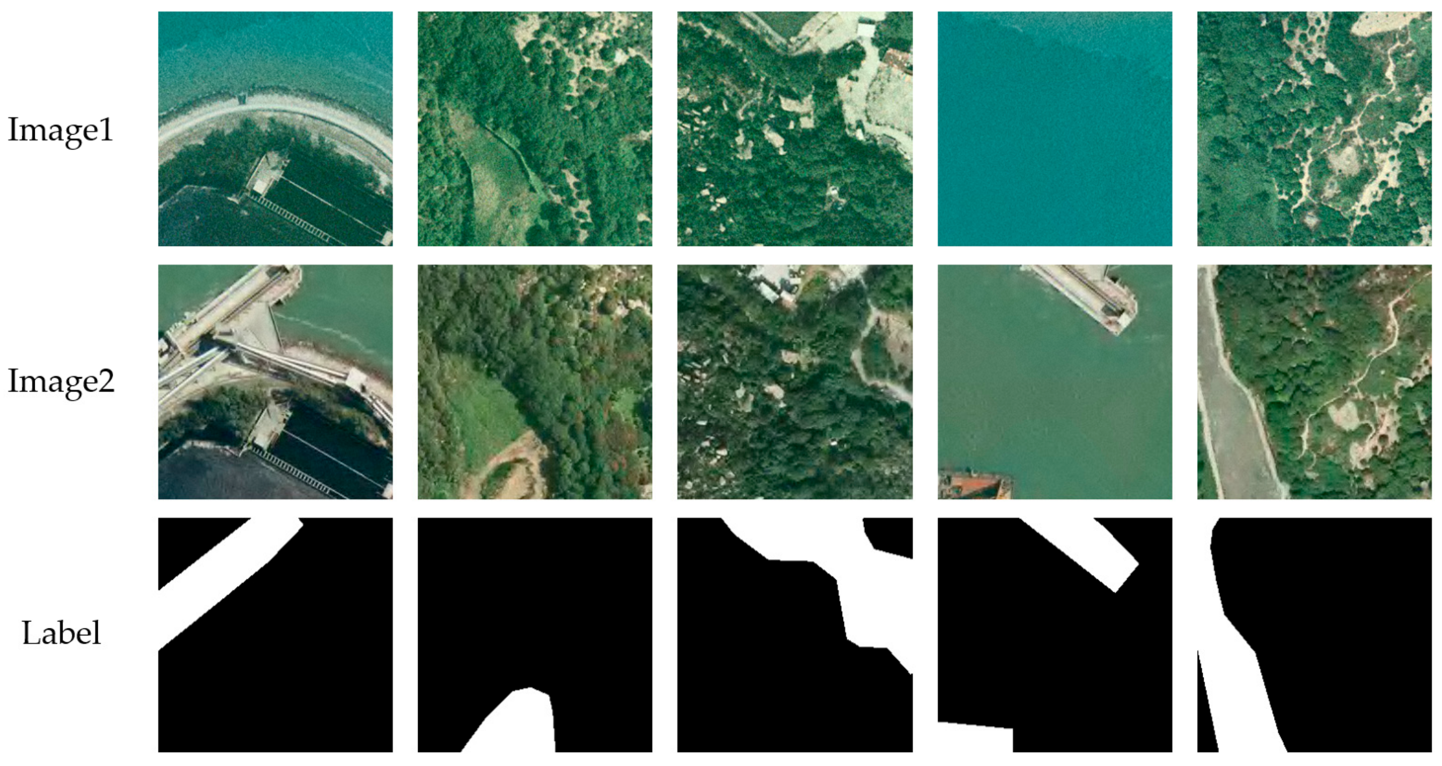
The SYSU-CD dataset comprises bitemporal aerial images taken in Hong Kong from 2007 to 2014, with a resolution of 0.5 GSD. It is a generic change detection dataset, and the primary change types include suburban expansion, building changes, pre-construction groundwork, vegetation changes, road expansion, and marine construction, among others. The dataset consists of 20,000 pairs of RGB images, each with a size of 256 × 256. The dataset is partitioned into a training set, validation set, and test set with a ratio of 6:2:2; Figure 5 shows several pairs of example images in SYSU-CD.

3.1.2. LEVIR-CD

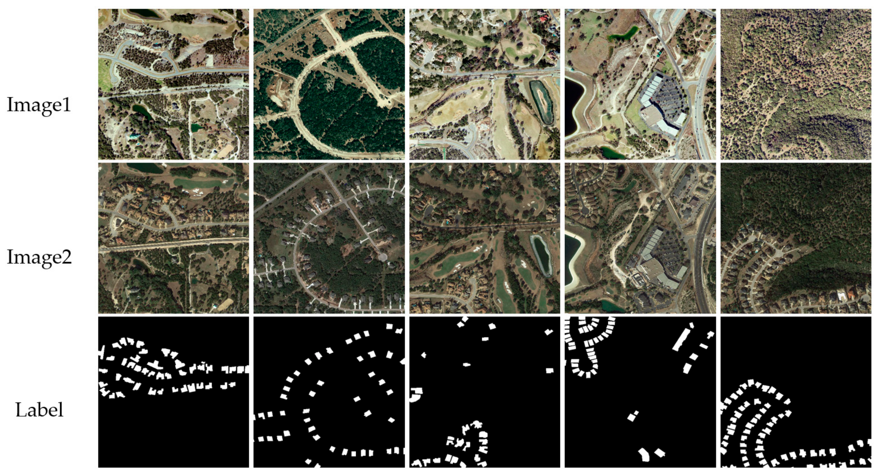
The LEVIR-CD dataset consists of 637 pairs of RGB images captured from 20 different areas in several cities in Texas, USA, from 2002 to 2018, with a resolution of 0.5 GSD. The dataset is specifically designed for building change detection and focuses only on changes in individual categories of buildings. The image size is 1024 × 1024, providing high spatial resolution for detailed analysis; Figure 6 shows several pairs of LEVIR-CD example images.

The profiles of SYSU-CD and LEVIR-CD are summarized in

Table 1. Overview of the dataset used in this paper.

Dataset	Type	GSD	Quantity of Trainset	Quantity of Valset	Quantity of Testset	Size
SYSU-CD	Generic	0.5 m	12,000 pairs	4000 pairs	4000 pairs	256 × 256
LEVIR-CD	Building	0.5 m	445 pairs	64 pairs	128 pairs	1024 × 1024

. GSD means ground sample distance. Both datasets exhibit significant class imbalance, with a positive-to-negative sample ratio of 1:4 in SYSU-CD and 1:20 in LEVIR-CD.

3.2. Evaluation Metrics

The evaluation metrics commonly used in change detection tasks are accuracy P (Precision) and recall R (Recall); P and R are calculated as follows:

$$P=\frac{TP}{TP+FP}$$

(12)

$$R=\frac{TP}{TP+FN}$$

(13)

where TP represents the number of true positive samples that are correctly identified as positive by the model; FP represents the number of false positive samples that are incorrectly identified as positive by the model; FN represents the number of false negative samples that are incorrectly identified as negative by the model; and TN represents the number of true negative samples that are correctly identified as negative by the model.

In practical applications, since P and R are two indicators that influence each other, this paper also uses the metric F1 score that combines the two measures, which is the harmonic mean of P and R. The calculation of F1 is as follows:

$$F1=2\times \frac{P\times R}{P+R}$$

(14)

In addition, in this paper, IOU is used as an evaluation metric. In change detection, there are only two categories of change and non-change, and this paper only calculates the IOU of the change category, which is calculated as follows:

$$IOU=\frac{TP}{TP+FP+FN}$$

(15)

3.3. Comparison Method

To verify the effectiveness of the proposed method, we compare MFNet with ten existing state-of-the-art algorithms, which are presented as follows:

FC-EF [7], FC-Siam-conc [7], and FC-Siam-diff [7] were proposed in 2018. They were the first algorithms that introduced Siamese networks to the change detection task. EF indicates early fusion, where the twin-temporal images are fused in the input phase; Siam-conc indicates a Siamese network-based splicing fusion model that fuses the bitemporal features of the Siamese network output using the concatenate operation; Siam-diff indicates a twin network-based difference fusion model.

STANet [1] was proposed in 2020. It uses a self-attention feature fusion module for change detection and captures spatiotemporal dependencies in multiple sub-regions of the image. The LEVIR-CD dataset is published in this paper.

BiT [12] was proposed in 2021. It uses Transformer as a fusion network of changing features based on the CNN backbone network to model the global semantic information of bitemporal features.

SNUNet [8] was proposed in 2021. It draws on the UNet++ network model to introduce multi-level dense connections in the decoder for change detection and integrates a channel attention mechanism to refine semantic features at different scales.

DSAMNet [18] was proposed in 2021. It uses a metric module with an integrated CBAM module for change prediction, along with additional supervised branches in the shallow network. The SYSU-CD dataset is published in this paper.

SSANet [37] was proposed in 2022. It was designed as a novel joint learning framework consisting of fusion sub-networks, differential networks, and decoders with an effective self-weighted spatiotemporal attention network.

ChangeFormer [13] was proposed in 2022. It introduces a pure Transformer architecture in the change detection task to efficiently obtain the multi-scale long-range details required for change detection.

USSFC-Net [38] was proposed in 2023. It includes a multiscale decoupled convolution (MSDConv), which can flexibly capture the multiscale features of changed objects. An efficient spatial–spectral feature cooperation (SSFC) strategy is introduced to obtain richer features.

3.4. Implementation Details

The experimental hardware environment is Intel Xeon Gold 6240 [email protected] GHz, 128 G RAM, and NVIDIA Quadro RTX8000, and the software environment is the Ubuntu 18.04.6 LTS operating system and the PyTorch deep learning framework based on Python.

In the experimental setup, the number of training iterations is 10k iterations, the optimizer is AdamW [39], the initial learning rate is set to 0.0001, and the warm-up strategy with linear learning rate is used for the first 1000 iterations, the learning rate decay strategy is poly, and a single GPU is used. When training on SYSU-CD, an input size of 256 × 256 with a batch size of 32 is used. When training on LEVIR-CD, input images with a size of 512 × 512 and batch size of 16 are used, which are cropped from the original image. We discuss the effect of different input sizes of LEVIR-CD on the model in Appendix A. For data augmentation, strategies such as random resize, random crop, random flip, random rotation, random color jitter, and input normalization are used. All augmentation strategies are used online during the model training process. The quantity and other details of the training data are shown in Table 1. The details for the data augmentation are shown in

Table 2. Details for data augmentation.

Data Augmentation	Arguments	Probability
resize	(0.5, 2.0)	1.0
crop	SYSU-CD: (256, 256) LEVIR-CD: (512, 512)	1.0
flip	up-down/left-right	0.5
rotation	(−90°, 90°)	0.5
color jitter	contrast-range = (0.5, 1.5) saturation-range = (0.5, 1.5)	0.5
normalization	mean = [123.675, 116.28, 103.53] std = [58.395, 57.12, 57.375]	1.0

.

In the experiments, to demonstrate the effectiveness of the proposed module, two different architectures are used as the encoder: ConvNeXt [40], based on a convolutional neural network, and Swin Transformer [41], based on self-attention, with ImageNet [42] image classification pre-training parameters and UperNet [43] structure for the decoder, using FP16 dynamic mixing accuracy during the training.

3.5. Quantitative Results

In this paper, two models MFNet-Conv and MFNet-SA are constructed based on convolutional neural networks and self-attention Transformer networks, respectively, where MFNet-Conv uses ConvNeXt-tiny as an encoder and MFNet-SA uses Swin-tiny as an encoder, in order to demonstrate the effectiveness of the proposed module in two different architectures.

Table 3. Quantitative evaluation results of different algorithms on SYSU-CD.

Methods	P (%)	R (%)	F1 (%)	IOU (%)
FC-EF [7]	81.61	69.63	75.13	60.18
FC-Siam-conc [7]	82.36	72.20	76.95	62.53
FC-Siam-diff [7]	63.58	87.08	73.50	58.11
STANet [16]	75.40	79.63	77.27	63.05
BiT [12]	68.78	88.45	77.39	63.12
SNUNet [8]	77.45	78.68	78.06	64.02
DSAMNet [18]	78.80	77.68	78.23	64.25
SSANet [37]	82.48	79.73	81.08	68.18
ChangeFormer [13]	82.78	81.23	81.99	70.36
MFNet-Conv (Ours)	89.40	77.64	83.11	71.10
MFNet-SA (Ours)	89.83	76.67	82.73	70.54

Color description: best, 2nd-best, 3rd-best.

and

Table 4. Quantitative evaluation results of different algorithms on LEVIR-CD.

Methods	P (%)	R (%)	F1 (%)	IOU (%)
FC-EF [7]	84.67	81.03	83.68	71.94
FC-Siam-conc [7]	92.64	76.89	84.03	72.46
FC-Siam-diff [7]	89.11	83.02	85.96	75.37
STANet [16]	87.99	87.65	87.82	77.51
BiT [12]	89.93	89.45	89.69	81.31
SNUNet [8]	89.14	86.73	87.92	78.45
DSAMNet [18]	80.19	89.06	84.39	73.01
SSANet [37]	91.71	90.53	91.12	83.69
ChangeFormer [13]	92.05	88.80	90.40	82.48
USSFC-Net [38]	89.70	92.42	91.04	\
MFNet-Conv (Ours)	91.69	91.05	91.37	84.11
MFNet-SA (Ours)	90.98	92.07	91.52	84.37

Color description: best, 2nd-best, 3rd-best.

show the quantitative evaluation results of the proposed method MFNet and several comparative algorithms on the LEVIR-CD and SYSU-CD datasets. The results in this paper are trained on the officially divided training set and tested on the test set without using additional data.

MFNet proposed in this paper produces competitive results compared with other algorithms and is substantially ahead of other algorithms on the generic change detection dataset SYSU-CD. MFNet-Conv achieves an F1 of 83.11% and an IOU of 71.10%, which is an improvement of 1.12% in F1 and 0.74% in IOU compared with the previous best method ChangeFormer. MFNet-SA is 0.38% smaller in F1 and 0.56% smaller in IOU than MFNet-Conv, but still achieves the second best result. On the building change detection dataset LEVIR-CD, MFNet-SA achieves an F1 of 91.52% and an IOU of 84.37%, which are 0.4% and 0.68% higher than SSANet, respectively, while MFNet-Conv achieves the second best result. However, the difference with the former is not large, because the ConvNeXt is an encoder optimized by the Transformer structure, and it can achieve an effect comparable to Transformer after adaptation. MFNet achieves the best metrics on both architectures and both datasets, illustrating its effectiveness.

3.6. Qualitative Results

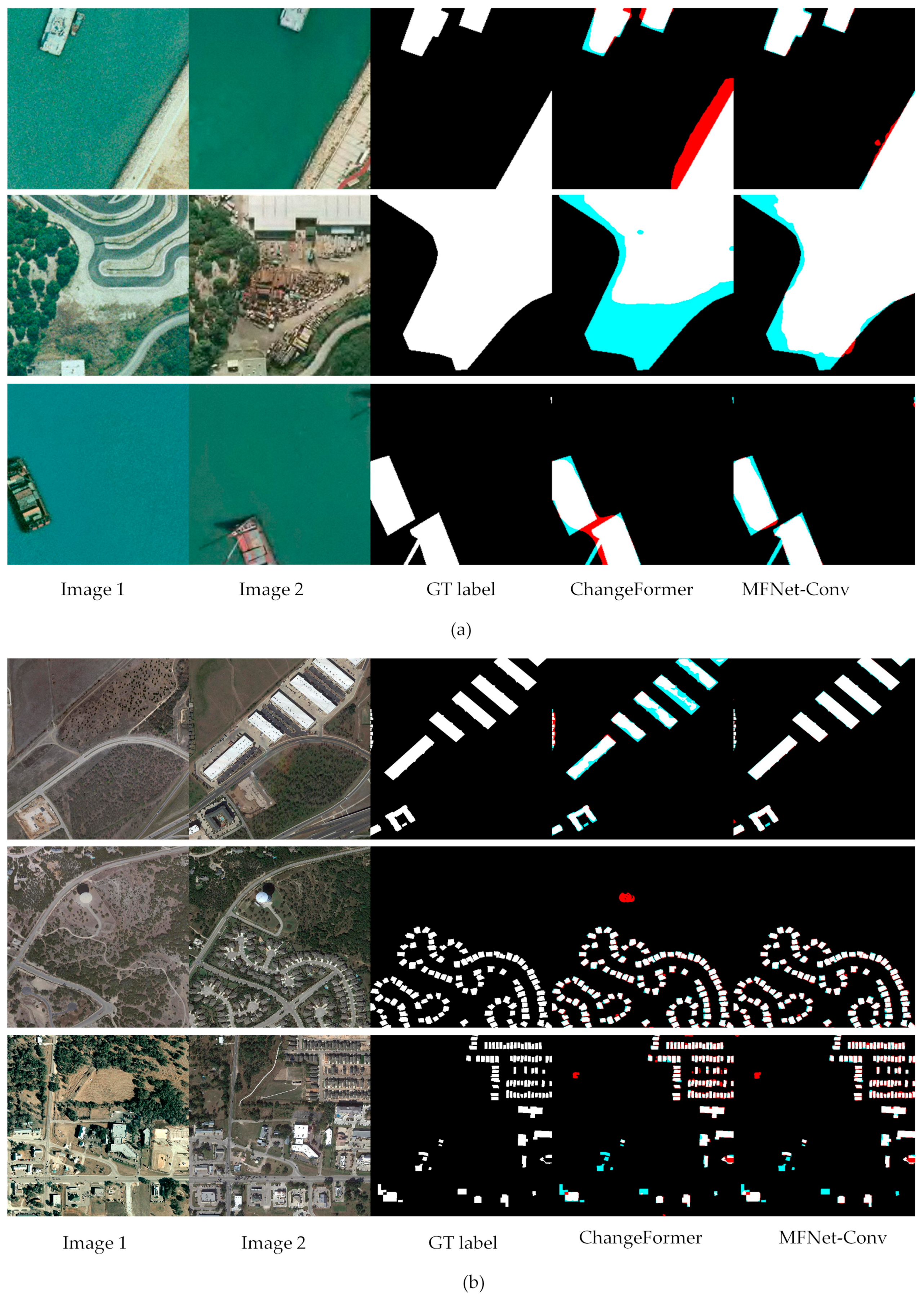
Figure 7 shows the prediction results of MFNet-Conv and ChangeFormer algorithms on SYSU-CD and LEVIR-CD. The first column in the figure shows the input image of the first temporal, the second column shows the input image of the second temporal, the third column shows the GT labels, the fourth column shows the prediction results of the ChangeFormer algorithm, and the last column shows the prediction results of MFNet-Conv. The red pixels in the prediction results indicate false positive detections and the blue pixels indicate false negative detections. It can be seen that, in the SYSU-CD dataset, the change pixels predicted by the method in this paper are significantly more accurate, for example, for the ship and land boundary in the first pair of images. MFNet can have fewer false detections and missed detections in the edge region compared to ChangeFormer and achieve high quality change detection. In the LEVIR-CD dataset, in the second pair of images, due to the light angle changes, a shadow of the ground water tower appears in different positions, which the ChangeFormer algorithm identifies as change, while MFNet is able to ignore this lighting change and correctly identify the real change area. Therefore, the proposed method MFNet has better performance and higher robustness.

4. Discussion

4.1. Ablation Experiment

In order to investigate the impact of each proposed module on the model’s performance, this subsection presents an ablation experimental analysis on the SYSU-CD dataset. The analysis aims to investigate the effect of each module on both MFNet-Conv and MFNet-SA. The results are presented in

Table 5. Results of MFNet ablation experiments on the SYSU-CD dataset.

Methods	SCFM	MFAM	Hybrid Loss	F1 (%)	IOU (%)
MFNet-Conv				81.52	69.87
	$\surd$			81.96 (+0.44)	70.21 (+0.34)
		$\surd$		82.38 (+0.86)	70.63 (+0.76)
			$\surd$	82.14 (+0.62)	70.47 (+0.60)
	$\surd$	$\surd$		82.64 (+1.12)	70.88 (+1.01)
	$\surd$	$\surd$	$\surd$	83.11 (+1.59)	71.10 (+1.23)
MFNet-SA				81.79	69.84
	$\surd$			82.04 (+0.25)	69.99 (+0.15)
		$\surd$		82.32 (+0.53)	70.27 (+0.43)
			$\surd$	82.11 (+0.32)	70.13 (+0.29)
	$\surd$	$\surd$		82.45 (+0.66)	70.38 (+0.54)
	$\surd$	$\surd$	$\surd$	82.73 (+0.94)	70.54 (+0.70)

, where SCFM, MFAM, and Hybrid Loss refer to the three optimization strategies proposed in this paper. The baseline model adopts the concatenate (Concat) operation as the change feature fusion method, and the binary cross entropy (BCE) loss function is used. Furthermore, there is no information exchange between the features of different time phases in the encoder stage.

The experimental results demonstrate that the three proposed improvements can effectively enhance the performance of both MFNet-Conv, which is based on a convolutional neural network, and MFNet-SA, which is based on a self-attention transformer. The F1 score of MFNet-Conv and MFNet-SA can be increased by 1.59% and 0.94%, respectively, compared to the baseline, while IOU is improved by 1.23% and 0.7%, respectively. Notably, the mutual feature-aware module MFAM brings the most significant improvement, with the F1 score increasing by 0.86% and IOU by 0.76% in MFNet-Conv, and the F1 score increasing by 0.53% and IOU by 0.43% in MFNet-SA. The improvement of the SA model is lower than that of the Conv model because the internal structure of the Conv model is a pure convolutional structure with a limited receptive field. The introduction of the MFAM module with a global receptive field on the top of it can bring more improvement. The overall metrics of the SA model are lower than those of the Conv model because the ConvNeXt model used in the Conv model itself is borrowed from the Swin model, which has better performance than Swin in terms of training strategy, model structure, and many other aspects. The experimental analysis presented here illustrates the quantitative influence of different modules on the model and verifies the rationality and effectiveness of the method design proposed in this paper.

Additionally,

Table 6. Results of ablation experiments with different fusion methods of change features on the SYSU-CD dataset.

Methods	Fusion	F1 (%)	IOU (%)
MFNet-Conv	Diff	80.23	67.45
	Concat	81.52	69.87
	SCFM	81.96	70.21

compares the symmetric change feature fusion module (SCFM) proposed with two other commonly used change feature fusion structures. The Diff method uses direct feature differencing, which results in the worst F1 score of only 80.23% due to the loss of more unrecoverable feature information during differencing. The Concat method uses concatenate feature fusion, which preserves the features entirely compared to Diff, and a convolutional layer with a 1 × 1 kernel size is used to learn the extraction of change features automatically. The F1 score obtained from Concat is 1.29% higher than that obtained from Diff. In contrast, the SCFM proposed in this paper achieves the best results by maintaining the symmetry of the network and obtaining the change feature prior via a difference branch without losing information. The F1 score obtained from SCFM is further improved by 0.44% compared to that obtained from Concat.

Table 7. Results of ablation experiments using MFAM at different stages of the encoder.

Methods	Stage 1	Stage 2	Stage 3	Stage 4	F1 (%)	IOU (%)
MFNet-Conv					81.52	69.87
			$\surd$	$\surd$	82.38	70.63
		$\surd$	$\surd$	$\surd$	82.13	70.35
	$\surd$	$\surd$	$\surd$	$\surd$	81.39	69.58

presents the results of ablation experiments conducted using the mutual feature-aware module MFAM at different stages of the encoder. The results show that the greatest improvement is achieved when the module is used after stage 3 and stage 4 of the deep network, resulting in a 0.86% and 0.76% improvement in the F1 score and IOU, respectively. However, it is important to note that introducing shallow feature interactions can lead to a decrease in performance, even worse than the baseline, as seen in the last two rows. This can be attributed to the fact that shallow features contain less semantic information, and the extraction of change features is less effective after bitemporal feature interaction, leading to noise in the network and resulting in performance degradation.

Table 8. Results of ablation experiments of CMSM in MFAM.

Methods	MFAM		F1 (%)	IOU (%)
	SCFM	CMSM
MFNet-Conv	MFAM is not used		81.52	69.87
	$\surd$		82.17	70.37
	$\surd$	$\surd$	82.38	70.63

presents the results of ablation experiments for the cross self-attention module CMSM structure in the mutual feature perception module MFAM. Without CMSM, adding the mutual features obtained using the symmetric change feature fusion module SCFM proposed above to the encoder backbone can improve the F1 score by 0.65%. With the addition of the CMSM structure to capture the global perceptual field, the F1 score can be further improved by 0.21%. These results confirm the effectiveness of the CMSM in improving the performance of the system.

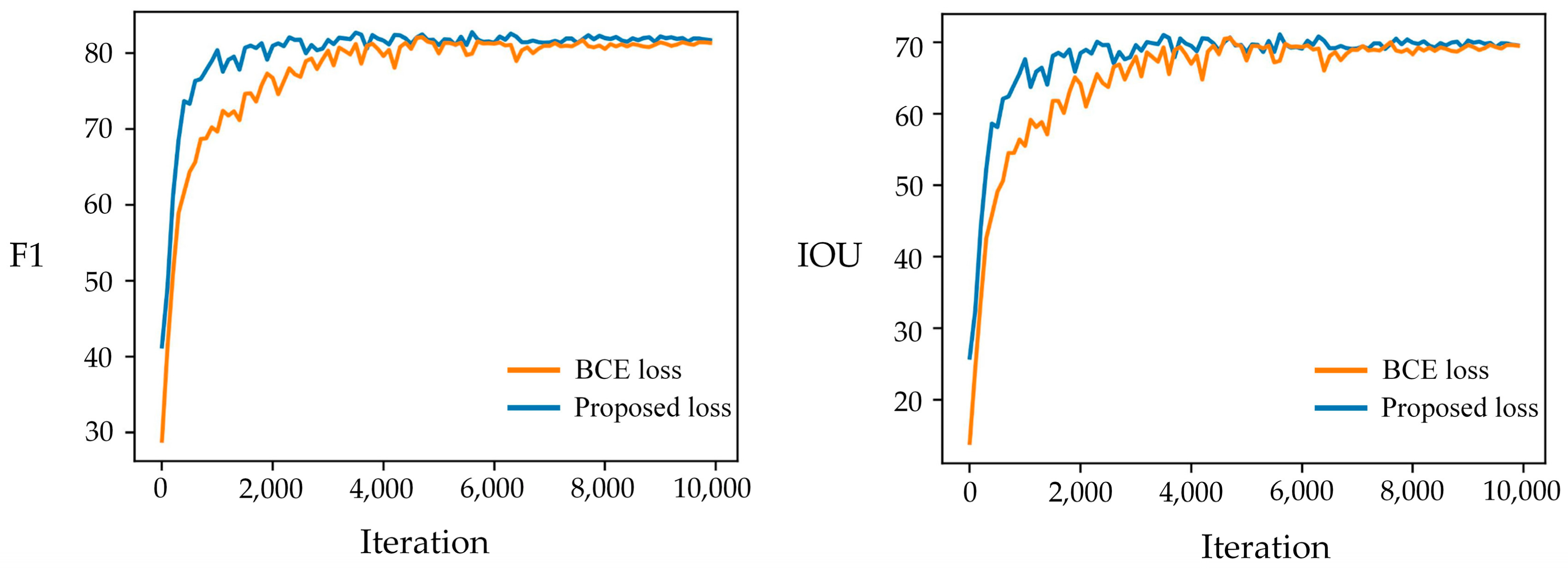
Figure 8 depicts the convergence rate of the F1 score and the IOU metrics of the MFNet-Conv model on SYSU-CD when utilizing different losses. The orange curve represents the usage of binary cross-entropy loss solely, whereas the blue curve corresponds to the employment of losses proposed in this paper, including the BCE loss with hard sample mining, Dice loss, and edge Dice, focusing on the edges of the change region. The horizontal axis of the curve signifies the number of iterations (iter), where the metrics evaluation is performed every 100 iterations, and the vertical axis indicates the evaluation metrics F1 score or IOU. The hybrid loss proposed in this paper exhibits a faster convergence rate, and, at 1000 iterations, the F1 metric attains 78.98%, and the IOU reaches 65.63%, reflecting improvements of 7.41% and 9.3% compared to BCE, respectively. Furthermore, Table 4 shows that in the final steady-state metrics, the hybrid loss surpasses BCE by 0.62% and 0.60% in the F1 score and IOU, respectively.

Table 9. Parameters and FLOPs for each module of MFNet-Conv.

Baseline	SCFM	MFAM	Params. (M)	FLOPs (G)	F1 (%)
$\surd$			48.98	41.64	81.52
$\surd$	$\surd$		49.37 (+0.39)	41.84 (+0.20)	81.96 (+0.44)
$\surd$		$\surd$ w.o.CMSM	52.30 (+3.32)	42.09 (+0.45)	82.17 (+0.65)
$\surd$		$\surd$ with CMSM	61.17 (+12.19)	43.00 (+1.36)	82.38 (+0.86)
$\surd$	$\surd$	$\surd$ with CMSM	61.56 (+12.58)	43.20 (+1.56)	82.64 (+1.12)

shows the parameters, FLOPs and F1 metrics on the SYSU-CD dataset for each module proposed in this paper. FLOPs are computed at an input scale of 256 × 256. It is evident from the table that the symmetric change feature fusion module SCFM only slightly increases the parameters by 0.39 M and FLOPs by 0.2 G. With only two 1 × 1 convolutions in the feature selection module and one 1 × 1 convolution in the H × W scale space in this structure, it is possible to obtain a 0.44% F1 score improvement with a very small increase in the number of parameters. On the other hand, the mutual feature-aware module MFAM has a larger number of parameters. When using the cross self-attention module CMSM, the number of parameters increases by 12.19 M, but the FLOPs only increase by 1.36 G. This module can be used with more abundant memory resources to achieve the best performance. However, under limited arithmetic resources, the CMSM structure can be removed, and, compared to the baseline, the number of parameters only increases by 3.32 M and the FLOPs increase by 0.45 G, which still results in a 0.65% F1 score improvement.

4.2. Feature Visualization

This subsection provides a visualization and analysis of the proposed mutual feature perception module MFAM and symmetric change feature fusion module SCFM, from a feature-based perspective.

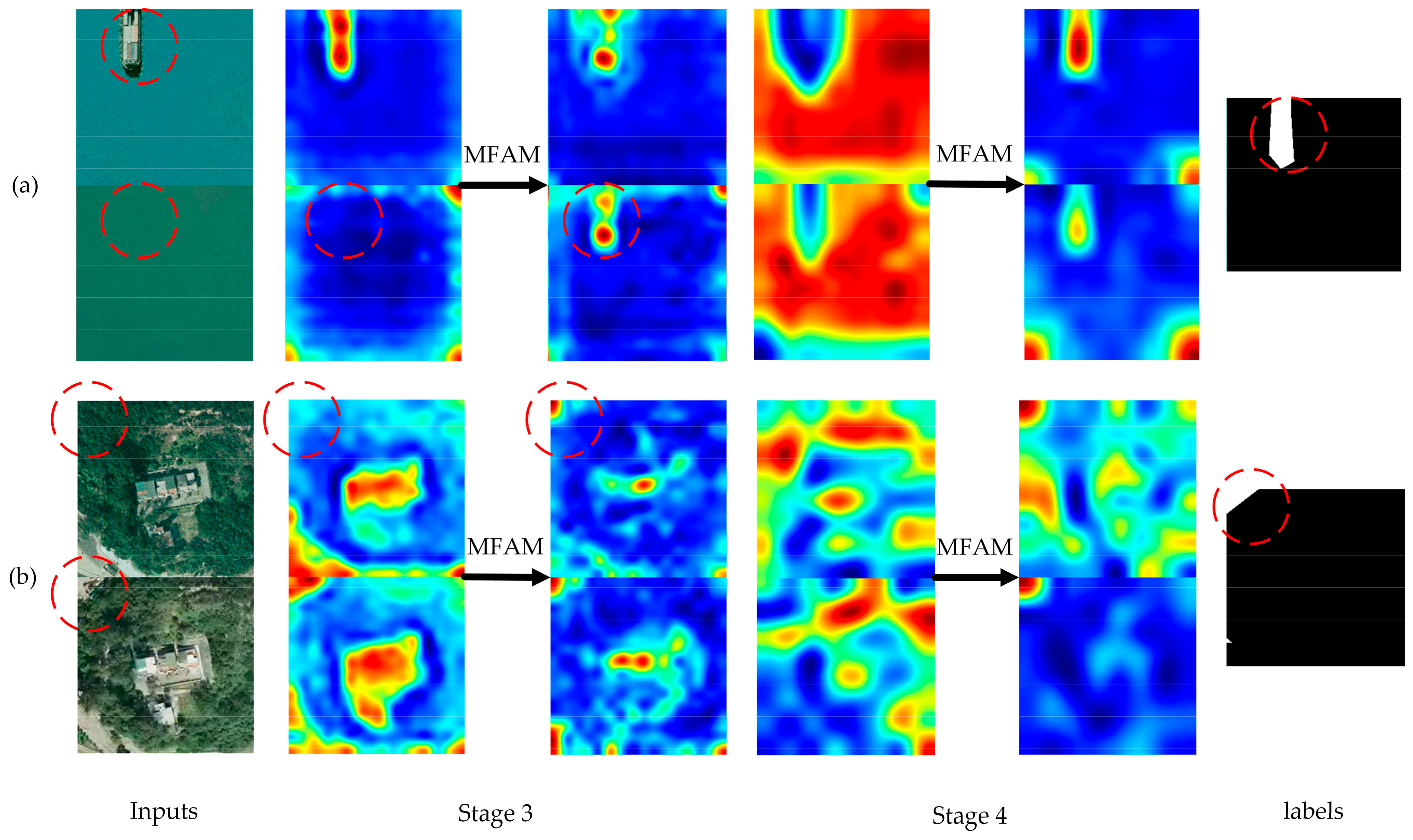
Figure 9 displays the feature visualization of the encoder’s features in the model at stage 3 and stage 4 before and after undergoing the proposed mutual feature-aware module process. Two pairs of images, Figure 9a and Figure 9b, are presented. The first row in Figure 9a exhibits the features of the pre-temporal image, while the second row shows the features of the post-temporal image. The second and third columns of both image pairs represent the features before and after the MFAM module of stage 3 of the encoder, while the fourth and fifth columns represent the features before and after the MFAM module of stage 4 of the encoder. From the figure, it is evident that, before MFAM in stage 3 of image pair Figure 9a, no higher corresponding feature exists because the post-temporal shadow map is solely a water surface. However, after MFAM in the feature map of the post-temporal phase, a higher response emerges at the position of the red dashed circle in the figure, which represents the region where the change occurs. This phenomenon is similarly observed in stage 4. Similarly, the same phenomenon occurs at stage 3 of image pair Figure 9b, where there is no response at the red dashed coil before MFAM. However, after MFAM, a higher response appears, and this is the region where the change occurs. Therefore, the mutual feature-aware module MFAM can enhance the focus on the changed region at the encoder stage, which enables the network to extract features in a more targeted manner.

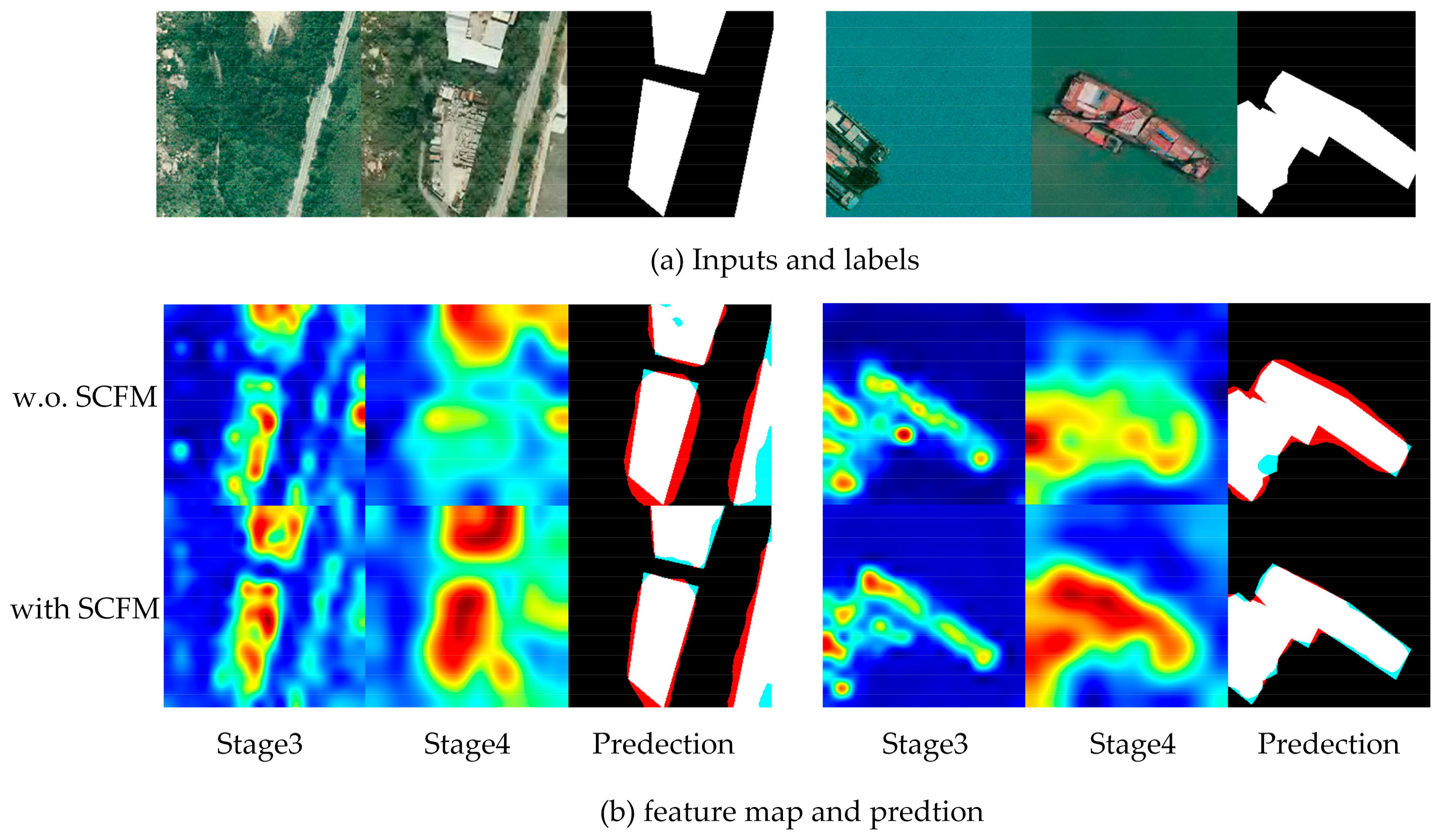
Figure 10 presents the feature visualization outcomes of the decoder at stage 3 and stage 4 regarding the symmetric change feature fusion module SCFM. The white color in the prediction results signifies true positive predictions (TP), while the red and blue colors correspond to false positive predictions (FP) and false negative predictions (FN), respectively. As shown in the figure, utilizing SCFM results in a stronger feature response in the change region, with most of the response concentrated in this area, and a weaker response in the non-change region. Comparing the feature response locations with the change detection prediction results, it is evident that more precise response locations lead to better change prediction accuracy. The employment of SCFM not only assists in accurately detecting changes, but also decreases false and missed detections in the edge regions. These observations demonstrate the effectiveness of the symmetric change feature fusion module SCFM.

4.3. Computational Complexity

This subsection compares the proposed algorithm MFNet with other algorithms from the point of view of computational complexity, mainly comparing parameters and FLOPs, which is computed with an input size of 256 × 256.

Table 10. Comparison of computational complexity and metrics on LEVIR-CD of different algorithms.

Methods	Params. (M)	FLOPs (G)	F1 (%)	IOU (%)
FC-EF [7]	1.35	3.56	83.68	71.94
FC-Siam-conc [7]	1.82	4.71	84.03	72.46
FC-Siam-diff [7]	2.03	5.32	85.96	75.37
STANet [16]	24.37	12.03	87.82	77.51
BiT [12]	22.87	26.31	89.69	81.31
SNUNet [8]	13.21	54.82	87.92	78.45
DSAMNet [18]	33.85	75.39	84.39	73.01
SSANet [37]	15.97	36.63	91.12	83.69
ChangeFormer [13]	41.01	101.42	90.40	82.48
USSFC-Net [38]	1.52	4.86	91.04	\
MFNet-Conv (Ours)	61.56	43.20	91.37	84.11
MFNet-SA (Ours)	74.75	67.05	91.52	84.37

shows the computational complexity of the different algorithms.

There is a constraint between the complexity and accuracy of the model for deep learning. Although the parameters and FLOPs of our method are larger, which is a limitation of our algorithm, it achieves the best performance in terms of accuracy. In addition, the FLOPs for our method are lower than for ChangeFormer.

5. Conclusions

In this paper, we propose MFNet, a mutual feature-aware network for remote sensing image change detection. Based on the encoder-decoder and Siamese network structure, we address three problems that exist in current remote sensing image change detection tasks, such as asymmetric change feature fusion, change feature extraction lag and sample imbalance and edge detection difficulties. A symmetric change feature fusion module SCFM, a mutual feature-aware module MFAM, and the edge loss function EL, are proposed, in which the symmetric change feature fusion module introduces the change feature a priori information using the two-branch feature selection without losing the feature information, and explicitly performs the spatial dimensional feature weighting based on the cosine similarity. The mutual feature-aware module introduces change features in advance at the encoder, allowing the model to target feature extraction for feature comparison in subsequent decoders. The edge loss guides the model to focus on the more difficult regions in the edge area, while alleviating the problem of unbalanced positive and negative samples.

We experimented on two commonly used change detection datasets, SYSU-CD and LEVIR-CD, and compared and analyzed them with the current mainstream remote sensing change detection algorithms. Detailed ablation experiments and feature visualization analysis were also performed to demonstrate the effectiveness of the proposed method.

In terms of future work to be carried out, in the mutual feature-aware module proposed in this paper, the intersection of the mutual features with the original features is performed by a simple concatenate operation plus a convolution operation, and more efficient structures for feature interaction can be explored in the future. Moreover, in order to improve the change detection performance, we use a heavy encoder in our method, which leads to the limitation of our method in terms of computational complexity, and cannot be applied in the case of restricted computational resources. For the next stage, we will study the lightweight remote sensing image change detection model under a computational resource constraint.

References

1. Asokan, A.; Anitha, J. Change detection techniques for remote sensing applications: A survey. Earth Sci. Inf. 2019, 12, 143–160. [Google Scholar] [CrossRef]
2. Jiang, H.; Hu, X.; Li, K.; Zhang, J.; Gong, J.; Zhang, M. PGA-SiamNet: Pyramid Feature-Based Attention-Guided Siamese Network for Remote Sensing Orthoimagery Building Change Detection. Remote Sens. 2020, 12, 484. [Google Scholar] [CrossRef]
3. Zhao, Y.; Feng, D.; Yu, L.; Cheng, Y.; Zhang, M.; Liu, X.; Xu, Y.; Fang, L.; Zhu, Z.; Gong, P. Long-Term Land Cover Dynamics (1986–2016) of Northeast China Derived from a Multi-Temporal Landsat Archive. Remote Sens. 2019, 11, 599. [Google Scholar] [CrossRef]
4. Sertel, E.; Ekim, B.; Ettehadi Osgouei, P.; Kabadayi, M.E. Land Use and Land Cover Mapping Using Deep Learning Based Segmentation Approaches and VHR Worldview-3 Images. Remote Sens. 2022, 14, 4558. [Google Scholar] [CrossRef]
5. Lu, C.-H.; Ni, C.-F.; Chang, C.-P.; Yen, J.-Y.; Chuang, R.Y. Coherence Difference Analysis of Sentinel-1 SAR Interferogram to Identify Earthquake-Induced Disasters in Urban Areas. Remote Sens. 2018, 10, 1318. [Google Scholar] [CrossRef]
6. Shi, W.; Zhang, M.; Zhang, R.; Chen, S.; Zhan, Z. Change Detection Based on Artificial Intelligence: State-of-the-Art and Challenges. Remote Sens. 2020, 12, 1688. [Google Scholar] [CrossRef]
7. Daudt, R.C.; Saux, B.L.; Boulch, A. Fully Convolutional Siamese Networks for Change Detection. In Proceedings of the 25th IEEE International Conference on Image Processing (ICIP), Athens, Greece, 7–10 October 2018; pp. 4063–4067. [Google Scholar] [CrossRef]
8. Fang, S.; Li, K.; Shao, J.; Li, Z. SNUNet-CD: A Densely Connected Siamese Network for Change Detection of VHR Images. IEEE Geosci. Remote Sens. Lett. 2022, 19, 8007805. [Google Scholar] [CrossRef]
9. Lyu, H.; Lu, H.; Mou, L. Learning a Transferable Change Rule from a Recurrent Neural Network for Land Cover Change Detection. Remote Sens. 2016, 8, 506. [Google Scholar] [CrossRef]
10. Chen, H.; Wu, C.; Du, B.; Zhang, L. Change Detection in Multisource VHR Images via Deep Siamese Convolutional Multiple-Layers Recurrent Neural Network. IEEE Trans. Geosci. Remote Sens. 2020, 58, 2848–2864. [Google Scholar] [CrossRef]
11. Khankeshizadeh, E.; Mohammadzadeh, A.; Moghimi, A. FCD-R2U-net: Forest change detection in bi-temporal satellite images using the recurrent residual-based U-net. Earth Sci. Inform. 2022, 15, 2335–2347. [Google Scholar] [CrossRef]
12. Chen, H.; Qi, Z.; Shi, Z. Remote Sensing Image Change Detection with Transformers. IEEE Trans. Geosci. Remote Sens. 2022, 60, 5607514. [Google Scholar] [CrossRef]
13. Bandara, W.G.C.; Patel, V.M. A Transformer-Based Siamese Network for Change Detection. In Proceedings of the IEEE International Geoscience and Remote Sensing Symposium, Kuala Lumpur, Malaysia, 17 July 2022; pp. 207–210. [Google Scholar] [CrossRef]
14. Chen, H.; Li, W.; Shi, Z. Adversarial Instance Augmentation for Building Change Detection in Remote Sensing Images. IEEE Trans. Geosci. Remote Sens. 2022, 60, 5603216. [Google Scholar] [CrossRef]
15. Jiang, H.; Peng, M.; Zhong, Y.; Xie, H.; Hao, Z.; Lin, J.; Ma, X.; Hu, X. A Survey on Deep Learning-Based Change Detection from High-Resolution Remote Sensing Images. Remote Sens. 2022, 14, 1552. [Google Scholar] [CrossRef]
16. Chen, H.; Shi, Z. A Spatial-Temporal Attention-Based Method and a New Dataset for Remote Sensing Image Change Detection. Remote Sens. 2020, 12, 1662. [Google Scholar] [CrossRef]
17. Peng, D.; Zhang, Y.; Guan, H. End-to-End Change Detection for High Resolution Satellite Images Using Improved UNet++. Remote Sens. 2019, 11, 1382. [Google Scholar] [CrossRef]
18. Shi, Q.; Liu, M.; Li, S.; Liu, X.; Wang, F.; Zhang, L. A Deeply Supervised Attention Metric-Based Network and an Open Aerial Image Dataset for Remote Sensing Change Detection. IEEE Trans. Geosci. Remote Sens. 2022, 60, 5604816. [Google Scholar] [CrossRef]
19. Chen, J.; Yuan, Z.; Peng, J.; Chen, L.; Huang, H.; Zhu, J.; Liu, Y.; Li, H. DASNet: Dual Attentive Fully Convolutional Siamese Networks for Change Detection in High-Resolution Satellite Images. IEEE J. Sel. Top Appl. Earth Obs. Remote Sensg. 2020, 14, 1194–1206. [Google Scholar] [CrossRef]
20. Zhang, C.; Yue, P.; Tapete, D.; Jiang, L.; Shangguan, B.; Huang, L.; Liu, G. A Deeply Supervised Image Fusion Network for Change Detection in High Resolution Bi-Temporal Remote Sensing Images. ISPRS J. Photogramm. Remote Sens. 2020, 166, 183–200. [Google Scholar] [CrossRef]
21. Ding, L.; Guo, H.; Liu, S.; Mou, L.; Zhang, J.; Bruzzone, L. Bi-Temporal Semantic Reasoning for the Semantic Change Detection in HR Remote Sensing Images. IEEE Trans. Geosci. Remote Sens. 2022, 60, 5620014. [Google Scholar] [CrossRef]
22. Diakogiannis, F.I.; Waldner, F.; Caccetta, P. Looking for Change? Roll the Dice and Demand Attention. Remote Sens. 2021, 13, 3707. [Google Scholar] [CrossRef]
23. Wang, Q.; Wu, B.; Zhu, P.; Li, P.; Zuo, W.; Hu, Q. ECA-Net: Efficient Channel Attention for Deep Convolutional Neural Networks. In Proceedings of the IEEE/CVF Conference on Computer Vision and Pattern Recognition, Seattle, MA, USA, 13–19 June 2020; pp. 11534–11542. [Google Scholar] [CrossRef]
24. Vaswani, A.; Shazeer, N.; Parmar, N.; Uszkoreit, J.; Jones, L.; Gomez, A.N.; Kaiser, L.; Polosukhin, I. Attention Is All You Need. In Proceedings of the Advances in Neural Information Processing Systems, Long Beach, CA, USA, 4–9 December 2017. [Google Scholar]
25. Xie, E.; Wang, W.; Yu, Z.; Anandkumar, A.; Alvarez, J.M.; Luo, P. SegFormer: Simple and Efficient Design for Semantic Segmentation with Transformers. In Proceedings of the Advances in Neural Information Processing System, Online, 6–11 December 2021; pp. 12077–12090. [Google Scholar]
26. Chen, P.; Zhang, B.; Hong, D.; Chen, Z.; Yang, X.; Li, B. FCCDN: Feature Constraint Network for VHR Image Change Detection. ISPRS J. Photogramm. Remote Sens. 2022, 187, 101–119. [Google Scholar] [CrossRef]
27. Zhu, Y.; Jin, G.; Liu, T.; Zheng, H.; Zhang, M.; Liang, S.; Liu, J.; Li, L. Self-Attention and Convolution Fusion Network for Land Cover Change Detection over a New Data Set in Wenzhou, China. Remote Sens. 2022, 14, 5969. [Google Scholar] [CrossRef]
28. Lin, T.-Y.; Dollar, P.; Girshick, R.; He, K.; Hariharan, B.; Belongie, S. Feature Pyramid Networks for Object Detection. In Proceedings of the 2017 IEEE Conference on Computer Vision and Pattern Recognition, Honolulu, HI, USA, 21–26 July 2017; pp. 936–944. [Google Scholar]
29. Hu, J.; Shen, L.; Sun, G. Squeeze-and-Excitation Networks. In Proceedings of the 2018 IEEE Conference on Computer Vision and Pattern Recognition, Salt Lake City, UT, USA, 18–23 June 2018; pp. 7132–7141. [Google Scholar] [CrossRef]
30. He, K.; Zhang, X.; Ren, S.; Sun, J. Deep Residual Learning for Image Recognition. In Proceedings of the 2016 IEEE Conference on Computer Vision and Pattern Recognition, Las Vegas, NV, USA, 27–30 June 2016; pp. 770–778. [Google Scholar]
31. Dong, X.; Bao, J.; Chen, D.; Zhang, W.; Yu, N.; Yuan, L.; Chen, D.; Guo, B. CSWin Transformer: A General Vision Transformer Backbone with Cross-Shaped Windows. In Proceedings of the 2022 IEEE Conference on Computer Vision and Pattern Recognition, New Orleans, LA, USA, 19–24 June 2022; pp. 12114–12124. [Google Scholar]
32. Dosovitskiy, A.; Beyer, L.; Kolesnikov, A.; Weissenborn, D.; Zhai, X.; Unterthiner, T.; Dehghani, M.; Minderer, M.; Heigold, G.; Gelly, S.; et al. An Image Is Worth 16x16 Words: Transformers for Image Recognition at Scale. In Proceedings of the International Conference on Learning Representations, Vienna, Austria, 30 April–3 May 2021. [Google Scholar]
33. Lebedev, M.A.; Vizilter, Y.V.; Vygolov, O.V.; Knyaz, V.A.; Rubis, A.Y. Change Detection in Remote Sensing Images Using Conditional Adversarial Networks. Int. Arch. Photogramm. Remote Sens. Spatial Inf. Sci. 2018, XLII–2, 565–571. [Google Scholar] [CrossRef]
34. Yang, K.; Xia, G.-S.; Liu, Z.; Du, B.; Yang, W.; Pelillo, M.; Zhang, L. Asymmetric Siamese Networks for Semantic Change Detection in Aerial Images. IEEE Trans. Geosci. Remote Sens. 2022, 60, 5609818. [Google Scholar] [CrossRef]
35. Ji, S.; Wei, S.; Lu, M. Fully Convolutional Networks for Multisource Building Extraction from an Open Aerial and Satellite Imagery Data Set. IEEE Trans. Geosci. Remote Sens. 2019, 57, 574–586. [Google Scholar] [CrossRef]
36. Shen, L.; Lu, Y.; Chen, H.; Wei, H.; Xie, D.; Yue, J.; Chen, R.; Lv, S.; Jiang, B. S2Looking: A Satellite Side-Looking Dataset for Building Change Detection. Remote Sens. 2021, 13, 5094. [Google Scholar] [CrossRef]
37. Jiang, K.; Zhang, W.; Liu, J.; Liu, F.; Xiao, L. Joint Variation Learning of Fusion and Difference Features for Change Detection in Remote Sensing Images. IEEE Trans. Geosci. Remote Sens. 2022, 60, 4709918. [Google Scholar] [CrossRef]
38. Lei, T.; Geng, X.; Ning, H.; Lv, Z.; Gong, M.; Jin, Y.; Nandi, A. Ultralightweight Spatial–Spectral Feature Cooperation Network for Change Detection in Remote Sensing Images. IEEE Trans. Geosci. Remote Sens. 2023, 61, 4402114. [Google Scholar] [CrossRef]
39. Loshchilov, I.; Hutter, F. Decoupled Weight Decay Regularization. In Proceedings of the International Conference on Learning Representations, New Orleans, LA, USA, 6–9 February 2019. [Google Scholar]
40. Liu, Z.; Mao, H.; Wu, C.-Y.; Feichtenhofer, C.; Darrell, T.; Xie, S. A ConvNet for the 2020s. In Proceedings of the 2022 IEEE Conference on Computer Vision and Pattern Recognition, New Orleans, LA, USA, 19–24 June 2022; pp. 11966–11976. [Google Scholar] [CrossRef]
41. Liu, Z.; Lin, Y.; Cao, Y.; Hu, H.; Wei, Y.; Zhang, Z.; Lin, S.; Guo, B. Swin Transformer: Hierarchical Vision Transformer Using Shifted Windows. In Proceedings of the 2021 IEEE International Conference on Computer Vision, Montreal, QC, Canada, 11–17 October 2021; pp. 9992–10002. [Google Scholar] [CrossRef]
42. Deng, J.; Dong, W.; Socher, R.; Li, L.-J.; Li, K.; Fei-Fei, L. ImageNet: A Large-Scale Hierarchical Image Database. In Proceedings of the 2009 IEEE Conference on Computer Vision and Pattern Recognition, Miami, FL, USA, 20–25 June 2009; pp. 248–255. [Google Scholar] [CrossRef]
43. Xiao, T.; Liu, Y.; Zhou, B.; Jiang, Y.; Sun, J. Unified Perceptual Parsing for Scene Understanding. In Proceedings of the European conference on computer vision, Munich, Germany, 8–14 September 2018; pp. 432–448. [Google Scholar] [CrossRef]
Figure 1. The overall architecture of the proposed MFNet.
Remotesensing 15 02145 g001
Figure 2. (a) Symmetric Change Feature Fusion Module; (b) Feature Selection Module; (c) Dissimilarity Weighting Module.
Remotesensing 15 02145 g002
Figure 3. (a) Mutual Feature-Aware Module; (b) Diagram of Cross Self-Attention (CSA); (c) Cross Multi-headed Self-attention Module.
Remotesensing 15 02145 g003
Figure 4. Schematic diagram of the edge Dice loss calculation area.
Remotesensing 15 02145 g004
Figure 5. Example of bitemporal input and labels in SYSU-CD.
Remotesensing 15 02145 g005
Figure 6. Example of bitemporal input and labels in LEVIR-CD.
Remotesensing 15 02145 g006
Figure 7. (a) Prediction results on SYSU-CD; (b) Prediction results on LEVIR-CD.
Remotesensing 15 02145 g007
Figure 8. Curve of IOU and F1 score under different loss.
Remotesensing 15 02145 g008
Figure 9. Feature visualization before and after the MFAM module. (a) and (b) denote the feature visualization of two pairs of images respectively. The red dashed circles show that the use of MFAM causes the encoder to focus on areas where changes may occur.
Remotesensing 15 02145 g009
Figure 10. Visualization of SCFM module features.
Remotesensing 15 02145 g010