

Global Mangrove Watch: Monthly Alerts of Mangrove Loss for Africa

 ,
,  ,
,  , ,
, ,
Abstract
:
1. Introduction
- Provide updates at least monthly, thereby allowing end users to respond to ongoing activities or be informed of natural events that compromise the integrity or existence of mangroves.
- Provide a low number of false positives; alerts might be ignored if false alerts are generated regularly.
- Provide a basis for an operational system; implemented in a suitable computing platform with a maintainable code base.
- To be computationally viable to scale to mangrove regions globally.
2. Background
3. Methods
3.1. Datasets
3.2. Mangrove Baseline
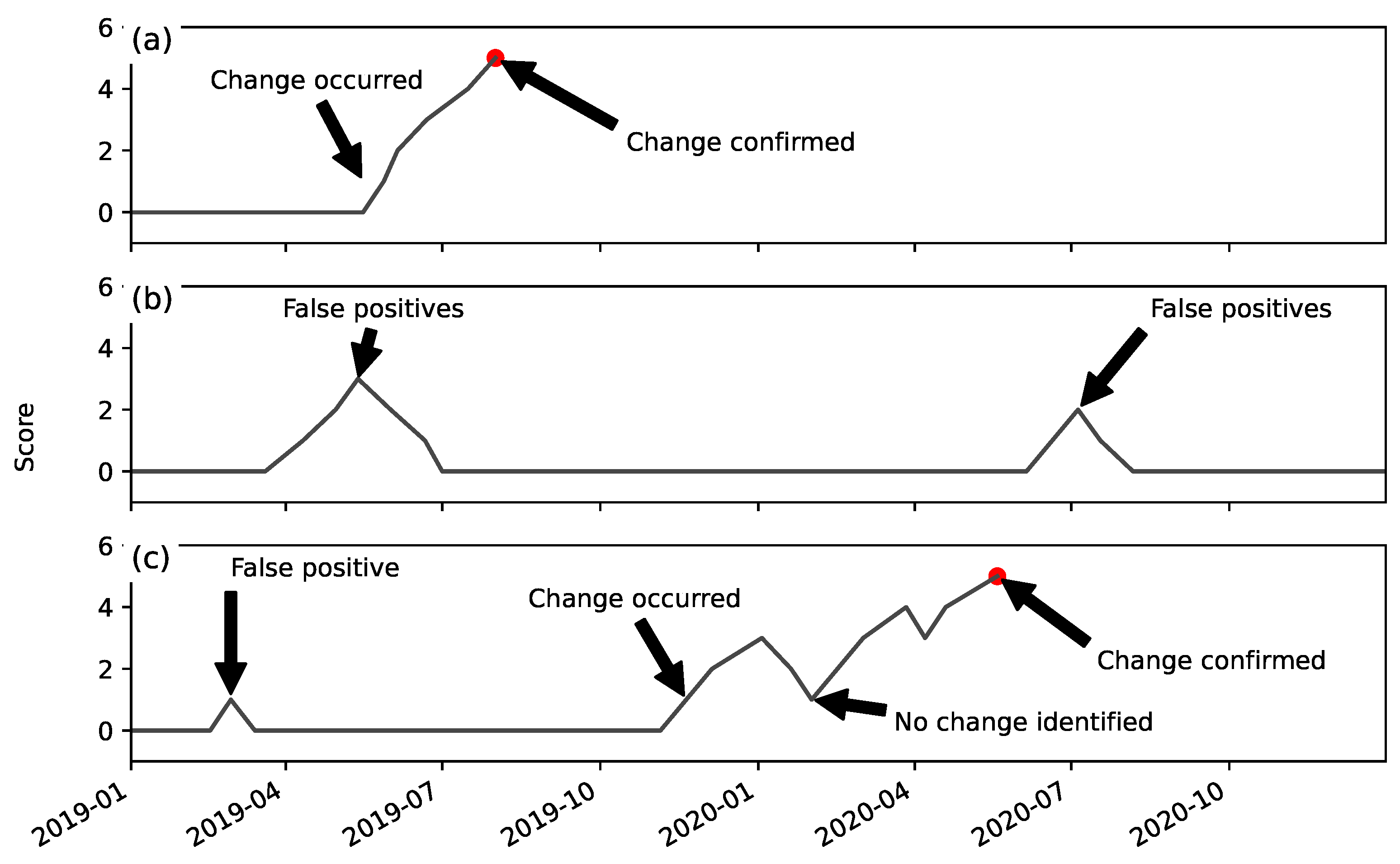
3.3. Identification of Mangrove Loss
3.4. Accuracy Assessment
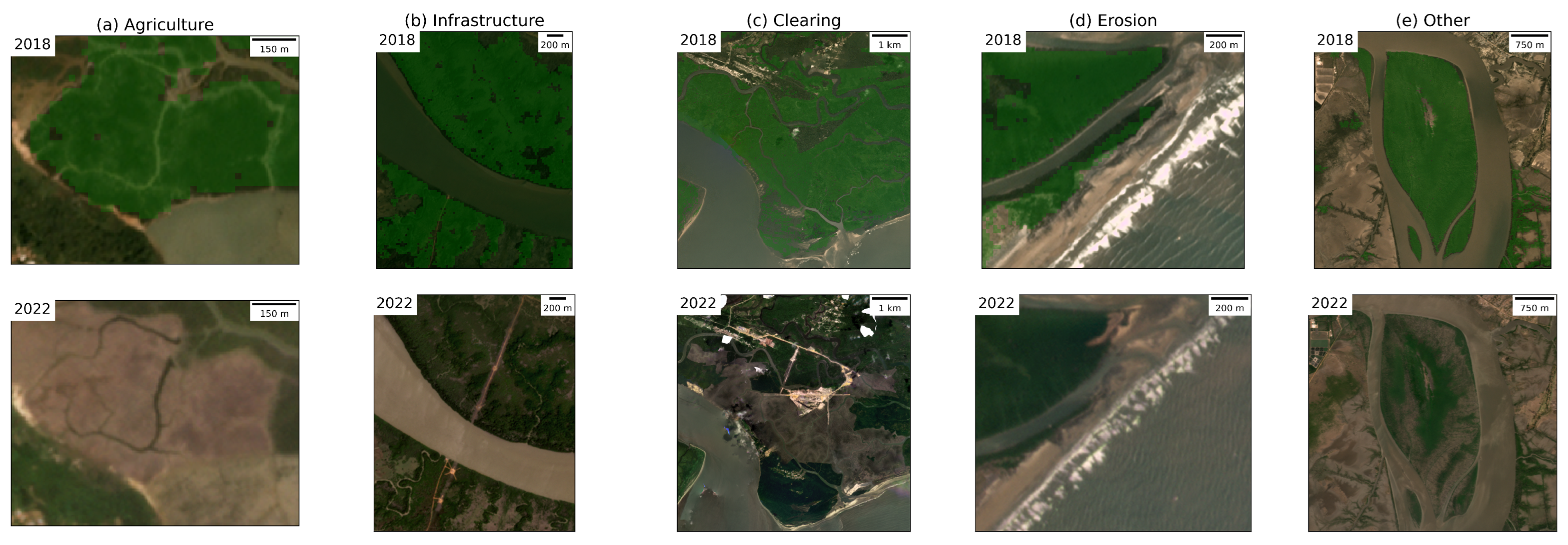
3.5. Causes of Change
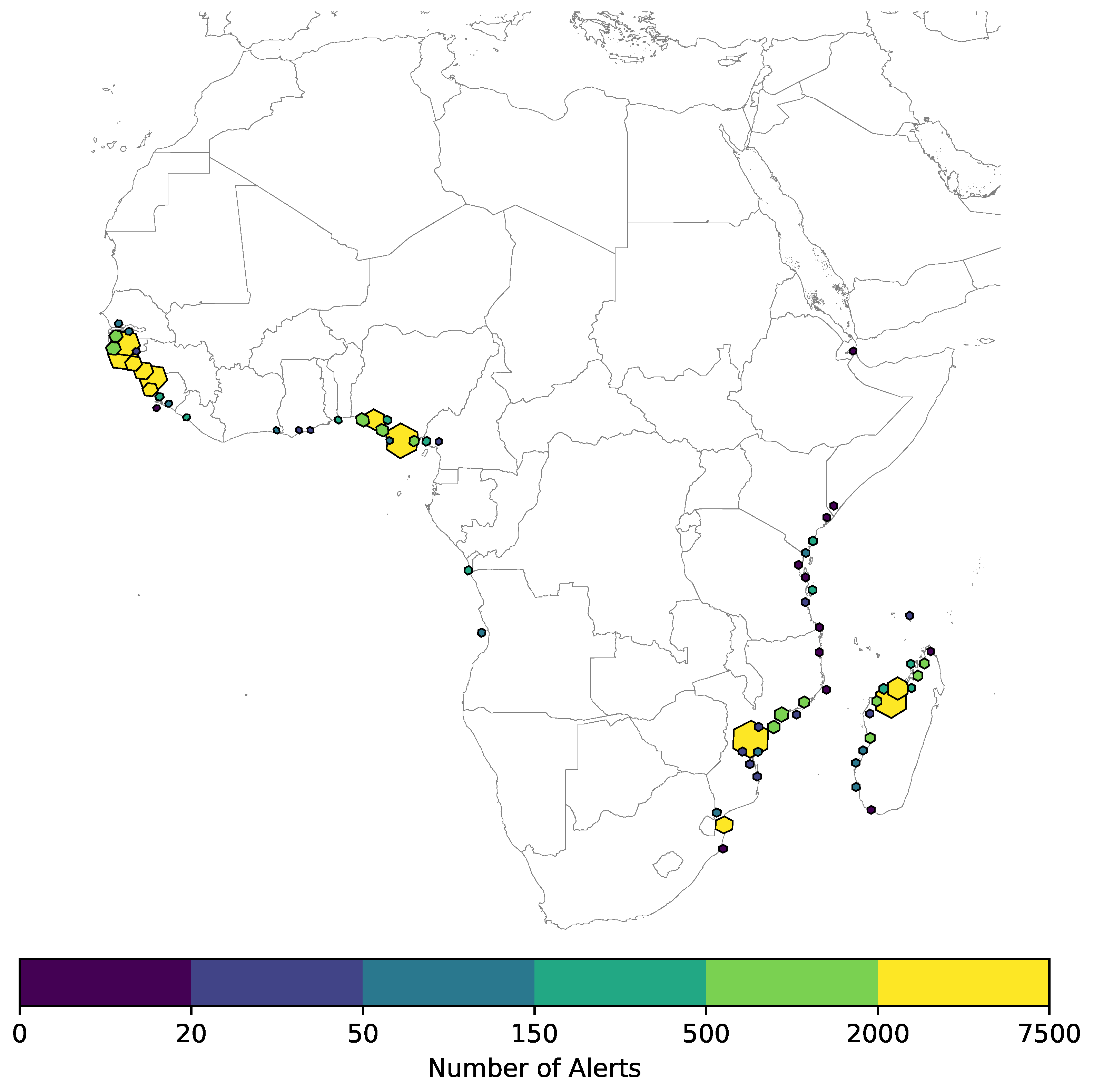
4. Results
4.1. Accuracy Assessment
4.2. Accuracy of Alert Timing
4.3. Comparison to JJ-FAST and GLAD Alerts
5. Discussion
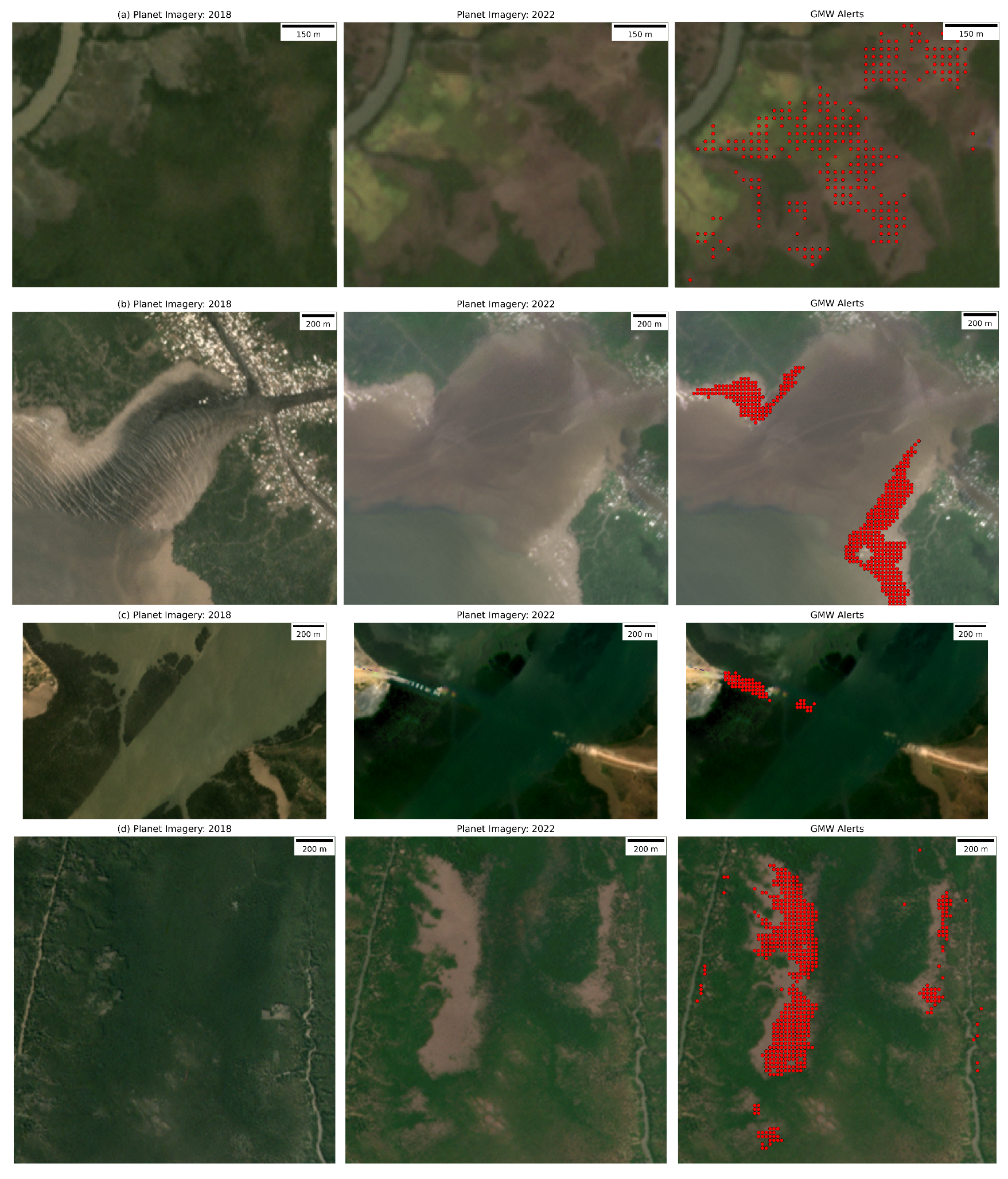
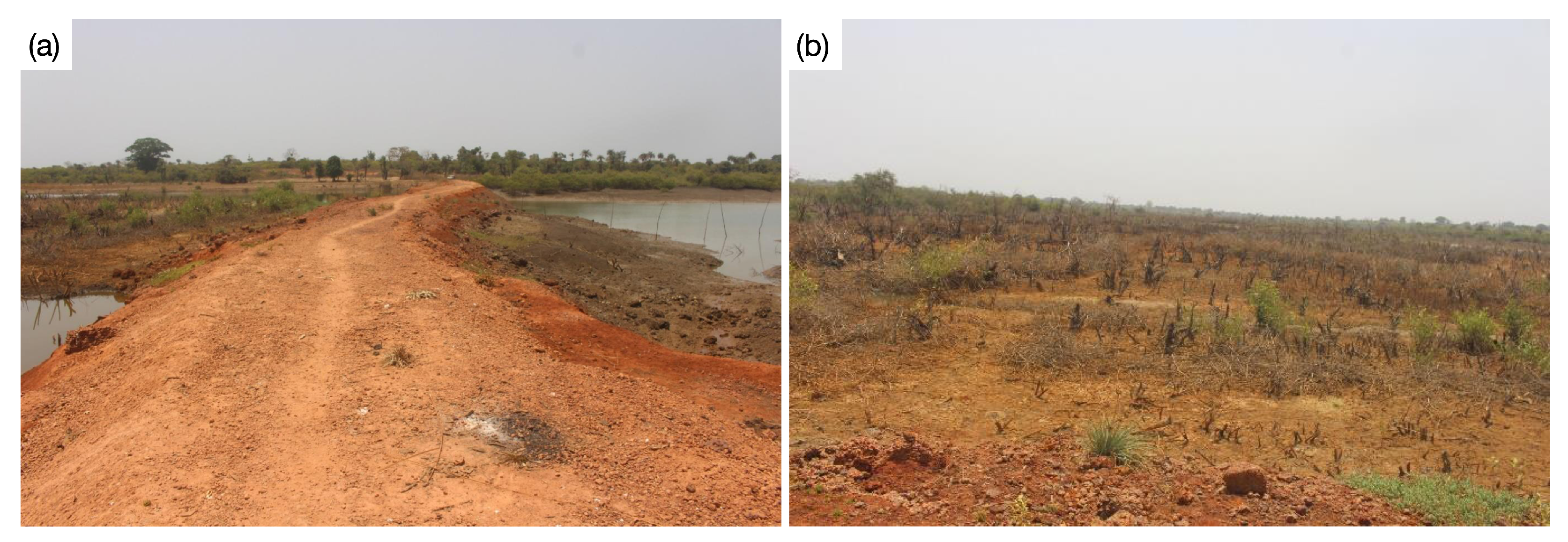
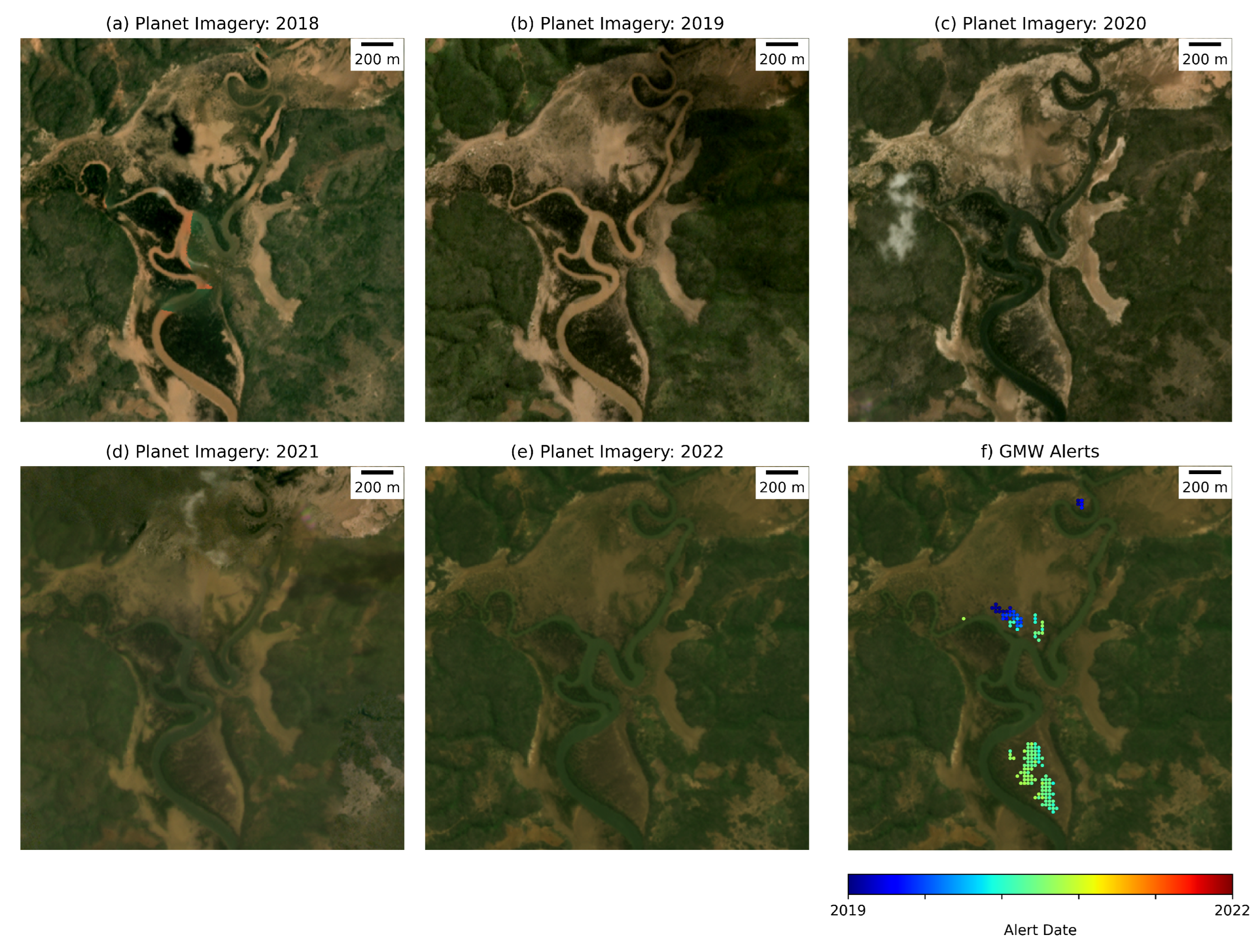
5.1. Case Study from Guinea-Bissau
5.2. Case Study from Kenya
5.3. Computational Scalability
5.4. Future Developments
6. Conclusions
Author Contributions
Funding
Data Availability Statement
Acknowledgments
Conflicts of Interest
References
- Agaton, C.B.; Collera, A.A. Now or later? Optimal timing of mangrove rehabilitation under climate change uncertainty. For. Ecol. Manag. 2022, 503, 119739. [Google Scholar] [CrossRef]
- Murray, N.J.; Worthington, T.A.; Bunting, P.; Duce, S.; Hagger, V.; Lovelock, C.E.; Lucas, R.; Saunders, M.I.; Sheaves, M.; Spalding, M.; et al. High-resolution mapping of losses and gains of Earth’s tidal wetlands. Science 2022, 376, 744–749. [Google Scholar] [CrossRef] [PubMed]
- Donato, D.C.; Kauffman, J.B.; Murdiyarso, D.; Kurnianto, S.; Stidham, M.; Kanninen, M. Mangroves among the most carbon-rich forests in the tropics. Nat. Geosci. 2011, 4, 293–297. [Google Scholar] [CrossRef]
- Simard, M.; Fatoyinbo, L.; Smetanka, C.; Rivera-Monroy, V.H.; Castañeda-Moya, E.; Thomas, N.; Stocken, T.V.d. Mangrove canopy height globally related to precipitation, temperature and cyclone frequency. Nat. Geosci. 2019, 12, 40–45. [Google Scholar] [CrossRef] [Green Version]
- Sievers, M.; Brown, C.J.; Tulloch, V.J.; Pearson, R.M.; Haig, J.A.; Turschwell, M.P.; Connolly, R.M. The Role of Vegetated Coastal Wetlands for Marine Megafauna Conservation. Trends Ecol. Evol. 2019, 34, 807–817. [Google Scholar] [CrossRef]
- Ermgassen, P.S.z.; Mukherjee, N.; Worthington, T.A.; Acosta, A.; Araujo, A.R.d.R.; Beitl, C.M.; Castellanos-Galindo, G.A.; Cunha-Lignon, M.; Dahdouh-Guebas, F.; Diele, K.; et al. Fishers who rely on mangroves: Modelling and mapping the global intensity of mangrove-associated fisheries. Estuar. Coast. Shelf Sci. 2021, 248, 107159. [Google Scholar] [CrossRef]
- Menéndez, P.; Losada, I.J.; Torres-Ortega, S.; Narayan, S.; Beck, M.W. The Global Flood Protection Benefits of Mangroves. Sci. Rep. 2020, 10, 4404. [Google Scholar] [CrossRef] [PubMed] [Green Version]
- Hochard, J.P.; Barbier, E.B.; Hamilton, S.E. Mangroves and coastal topography create economic “safe havens” from tropical storms. Sci. Rep. 2021, 11, 15359. [Google Scholar] [CrossRef] [PubMed]
- Spalding, M.; Parrett, C.L. Global patterns in mangrove recreation and tourism. Mar. Policy 2019, 110, 103540. [Google Scholar] [CrossRef]
- Thomas, N.; Lucas, R.; Bunting, P.; Hardy, A.; Rosenqvist, A.; Simard, M. Distribution and drivers of global mangrove forest change, 1996–2010. PLoS ONE 2017, 12, e0179302. [Google Scholar] [CrossRef] [Green Version]
- Friess, D.A.; Rogers, K.; Lovelock, C.E.; Krauss, K.W.; Hamilton, S.E.; Lee, S.Y.; Lucas, R.; Primavera, J.; Rajkaran, A.; Shi, S. The State of the World’s Mangrove Forests: Past, Present, and Future. Annu. Rev. Environ. Resour. 2019, 44, 1–27. [Google Scholar] [CrossRef] [Green Version]
- Wilkie, M.L.; Fortuna, S. Status and Trends in Mangrove Area Extent Worldwide; Technical Report; The Food and Agriculture Organization (FAO): Rome, Italy, 2003; Available online: http://www.fao.org/3/j1533e/J1533E02.htm (accessed on 12 December 2022).
- Wilkie, M.L.; Fortuna, S. Forest Resources Assessment (FRA) 2005 Thematic Study on Mangroves; Technical Report; Forest Resources Division, Food and Agriculture Organization of the United Nations: Rome, Italy, 2007. [Google Scholar]
- Global Mangrove Alliance. Available online: https://www.mangrovealliance.org (accessed on 12 December 2022).
- Bunting, P.; Rosenqvist, A.; Hilarides, L.; Lucas, R.M.; Thomas, N.; Tadono, T.; Worthington, T.A.; Spalding, M.; Murray, N.J.; Rebelo, L.M. Global Mangrove Extent Change 1996–2020: Global Mangrove Watch Version 3.0. Remote Sens. 2022, 14, 3657. [Google Scholar] [CrossRef]
- Bunting, P.; Rosenqvist, A.; Hilarides, L.; Lucas, R.M.; Thomas, N. Global Mangrove Watch: Updated 2010 Mangrove Forest Extent (v2.5). Remote Sens. 2022, 14, 1034. [Google Scholar] [CrossRef]
- Bunting, P.; Rosenqvist, A.; Lucas, R.; Rebelo, L.M.; Hilarides, L.; Thomas, N.; Hardy, A.; Itoh, T.; Shimada, M.; Finlayson, M. Global Mangrove Watch (1996–2016) Version 2.0; Zenodo: Genève, Switzerland, 2019. [Google Scholar] [CrossRef]
- Bunting, P.; Rosenqvist, A.; Lucas, R.; Rebelo, L.M.; Hilarides, L.; Thomas, N.; Hardy, A.; Itoh, T.; Shimada, M.; Finlayson, C. The Global Mangrove Watch—A New 2010 Global Baseline of Mangrove Extent. Remote Sens. 2018, 10, 1669. [Google Scholar] [CrossRef] [Green Version]
- Global Mangrove Watch Portal. Available online: https://globalmangrovewatch.org (accessed on 12 December 2022).
- Worthington, T.A.; Andradi-Brown, D.A.; Bhargava, R.; Buelow, C.; Bunting, P.; Duncan, C.; Fatoyinbo, L.; Friess, D.A.; Goldberg, L.; Hilarides, L.; et al. Harnessing Big Data to Support the Conservation and Rehabilitation of Mangrove Forests Globally. One Earth 2020, 3, 260. [Google Scholar] [CrossRef]
- Camberlin, P. Climate of Eastern Africa. In Oxford Research Encyclopedia of Climate Science; Oxford University Press: Oxford, UK, 2018. [Google Scholar] [CrossRef]
- Verburg, P.H.; Neumann, K.; Nol, L. Challenges in using land use and land cover data for global change studies. Glob. Chang. Biol. 2011, 17, 974–989. [Google Scholar] [CrossRef] [Green Version]
- Hansen, M.C.; Potapov, P.V.; Moore, R.; Hancher, M.; Turubanova, S.A.; Tyukavina, A.; Thau, D.; Stehman, S.V.; Goetz, S.J.; Loveland, T.R.; et al. High-Resolution Global Maps of 21st-Century Forest Cover Change. Science 2013, 342, 850–853. [Google Scholar] [CrossRef] [Green Version]
- Awty-Carroll, K.; Bunting, P.; Hardy, A.; Bell, G. Evaluation of the Continuous Monitoring of Land Disturbance Algorithm for Large-Scale Mangrove Classification. Remote Sens. 2021, 13, 3978. [Google Scholar] [CrossRef]
- Serra, P.; Pons, X.; Saurí, D. Post-classification change detection with data from different sensors: Some accuracy considerations. Int. J. Remote Sens. 2003, 24, 3311–3340. [Google Scholar] [CrossRef]
- Tewkesbury, A.P.; Comber, A.J.; Tate, N.J.; Lamb, A.; Fisher, P.F. A critical synthesis of remotely sensed optical image change detection techniques. Remote Sens. Environ. 2015, 160, 1–14. [Google Scholar] [CrossRef] [Green Version]
- Verbesselt, J.; Hyndman, R.; Newnham, G.; Culvenor, D. Detecting trend and seasonal changes in satellite image time series. Remote Sens. Environ. 2010, 114, 106–115. [Google Scholar] [CrossRef]
- Verbesselt, J.; Zeileis, A.; Herold, M. Near real-time disturbance detection using satellite image time series. Remote Sens. Environ. 2012, 123, 98–108. [Google Scholar] [CrossRef]
- Zhu, Z.; Woodcock, C.E. Continuous change detection and classification of land cover using all available Landsat data. Remote Sens. Environ. 2014, 144, 152–171. [Google Scholar] [CrossRef] [Green Version]
- Zhu, Z.; Zhang, J.; Yang, Z.; Aljaddani, A.H.; Cohen, W.B.; Qiu, S.; Zhou, C. Continuous monitoring of land disturbance based on Landsat time series. Remote Sens. Environ. 2020, 238, 111116. [Google Scholar] [CrossRef]
- Awty-Carroll, K.; Bunting, P.; Hardy, A.; Bell, G. Using Continuous Change Detection and Classification of Landsat Data to Investigate Long-Term Mangrove Dynamics in the Sundarbans Region. Remote Sens. 2019, 11, 2833. [Google Scholar] [CrossRef] [Green Version]
- Hansen, M.C.; Krylov, A.; Tyukavina, A.; Potapov, P.V.; Turubanova, S.; Zutta, B.; Ifo, S.; Margono, B.; Stolle, F.; Moore, R. Humid tropical forest disturbance alerts using Landsat data. Environ. Res. Lett. 2016, 11, 034008. [Google Scholar] [CrossRef]
- Reiche, J.; Mullissa, A.; Slagter, B.; Gou, Y.; Tsendbazar, N.E.; Odongo-Braun, C.; Vollrath, A.; Weisse, M.J.; Stolle, F.; Pickens, A.; et al. Forest disturbance alerts for the Congo Basin using Sentinel-1. Environ. Res. Lett. 2021, 16, 024005. [Google Scholar] [CrossRef]
- Watanabe, M.; Koyama, C.N.; Hayashi, M.; Nagatani, I.; Tadono, T.; Shimada, M. Refined algorithm for forest early warning system with ALOS-2/PALSAR-2 ScanSAR data in tropical forest regions. Remote Sens. Environ. 2021, 265, 112643. [Google Scholar] [CrossRef]
- Hammer, D.; Kraft, R.; Wheeler, D. Alerts of forest disturbance from MODIS imagery. Int. J. Appl. Earth Obs. Geoinf. 2014, 33, 1–9. [Google Scholar] [CrossRef]
- Shimabukuro, Y.E.; Santos, J.R.d.; Formaggio, A.R.; Duarte, V.; Rudorff, B.F.T. The Brazilian Amazon Monitoring Program: PRODES and DETER Projects. In Global Forest Monitoring from Earth Observation; Achard, F., Hansen, M.C., Eds.; Taylor & Francis: Abingdon, UK, 2016; Chapter 9; pp. 153–169. [Google Scholar]
- Microsoft Planetary Computer. Available online: https://planetarycomputer.microsoft.com (accessed on 12 December 2022).
- McFarland, M.; Emanuele, R.; Morris, D.; Augspurger, T. Microsoft Open Source: Microsoft/PlanetaryComputer: October 2022 (2022.10.28); Zenodo: Genève, Switzerland, 2022. [Google Scholar] [CrossRef]
- STAC. STAC: SpatioTemporal Asset Catalogs. 2022. Available online: https://stacspec.org (accessed on 14 November 2022).
- Project Jupyter. Available online: https://jupyter.org (accessed on 9 March 2023).
- Kubernetes. Available online: https://kubernetes.io/ (accessed on 9 March 2023).
- Rocklin, M. Dask: Parallel Computation with Blocked algorithms and Task Scheduling. In Proceedings of the 14th Python in Science Conference, Austin, TX, USA, 6–12 July 2015; pp. 130–136. [Google Scholar]
- Hoyer, S.; Hamman, J. Xarray: N-D labeled arrays and datasets in Python. J. Open Res. Softw. 2017, 5. [Google Scholar] [CrossRef] [Green Version]
- Open Data Cube STAC API. Available online: https://github.com/opendatacube/odc-stac (accessed on 18 December 2022).
- Main-Knorn, M.; Pflug, B.; Louis, J.; Debaecker, V.; Müller-Wilm, U.; Gascon, F. Sen2Cor for Sentinel-2. Image Signal Process. Remote Sens. XXIII 2017, 10427, 1042704. [Google Scholar] [CrossRef] [Green Version]
- Small, D. Flattening Gamma: Radiometric Terrain Correction for SAR Imagery. IEEE Trans. Geosci. Remote Sens. 2011, 49, 3081–3093. [Google Scholar] [CrossRef]
- Shimada, M.; Itoh, T.; Motooka, T.; Watanabe, M.; Shiraishi, T.; Thapa, R.; Lucas, R. New global forest/non-forest maps from ALOS PALSAR data (2007–2010). Remote Sens. Environ. 2014, 155, 13–31. [Google Scholar] [CrossRef]
- PALSAR-2 Mosaic Description v2.1.2. Available online: https://www.eorc.jaxa.jp/ALOS/en/dataset/pdf/DatasetDescription_PALSAR2_Mosaic_ver212.pdf (accessed on 18 December 2022).
- Baloloy, A.B.; Blanco, A.C.; Ana, R.R.C.S.; Nadaoka, K. Development and application of a new mangrove vegetation index (MVI) for rapid and accurate mangrove mapping. ISPRS J. Photogramm. Remote Sens. 2020, 166, 95–117. [Google Scholar] [CrossRef]
- Birch, C.P.; Oom, S.P.; Beecham, J.A. Rectangular and hexagonal grids used for observation, experiment and simulation in ecology. Ecol. Model. 2007, 206, 347–359. [Google Scholar] [CrossRef]
- Norway’s International Climate and Forests Initiative Satellite Data Program. Available online: https://www.planet.com/nicfi/ (accessed on 18 December 2022).
- Osuji, L.C.; Erondu, E.S.; Ogali, R.E. Upstream Petroleum Degradation of Mangroves and Intertidal Shores: The Niger Delta Experience. Chem. Biodivers. 2010, 7, 116–128. [Google Scholar] [CrossRef] [PubMed]
- Mentaschi, L.; Vousdoukas, M.I.; Pekel, J.F.; Voukouvalas, E.; Feyen, L. Global long-term observations of coastal erosion and accretion. Sci. Rep. 2018, 8, 12876. [Google Scholar] [CrossRef] [PubMed] [Green Version]
- Winterwerp, J.C.; Albers, T.; Anthony, E.J.; Friess, D.A.; Mancheño, A.G.; Moseley, K.; Muhari, A.; Naipal, S.; Noordermeer, J.; Oost, A.; et al. Managing erosion of mangrove-mud coasts with permeable dams–lessons learned. Ecol. Eng. 2020, 158, 106078. [Google Scholar] [CrossRef]
- Asbridge, E.; Lucas, R.; Rogers, K.; Accad, A. The extent of mangrove change and potential for recovery following severe Tropical Cyclone Yasi, Hinchinbrook Island, Queensland, Australia. Ecol. Evol. 2018, 8, 10416–10434. [Google Scholar] [CrossRef] [Green Version]
- Krauss, K.W.; Osland, M.J. Tropical cyclones and the organization of mangrove forests: A review. Ann. Bot. 2019, 125, 213–234. [Google Scholar] [CrossRef] [Green Version]
- Sandilyan, S.; Kathiresan, K. Decline of mangroves—A threat of heavy metal poisoning in Asia. Ocean Coast. Manag. 2014, 102, 161–168. [Google Scholar] [CrossRef]
- Krauss, K.W.; McKee, K.L.; Lovelock, C.E.; Cahoon, D.R.; Saintilan, N.; Reef, R.; Chen, L. How mangrove forests adjust to rising sea level. New Phytol. 2014, 202, 19–34. [Google Scholar] [CrossRef] [PubMed] [Green Version]
- Saintilan, N.; Lymburner, L.; Wen, L.; Haigh, I.D.; Ai, E.; Kelleway, J.J.; Rogers, K.; Pham, T.D.; Lucas, R. The lunar nodal cycle controls mangrove canopy cover on the Australian continent. Sci. Adv. 2022, 8, eabo6602. [Google Scholar] [CrossRef] [PubMed]
- Charrua, A.B.; Padmanaban, R.; Cabral, P.; Bandeira, S.; Romeiras, M.M. Impacts of the Tropical Cyclone Idai in Mozambique: A Multi-Temporal Landsat Satellite Imagery Analysis. Remote Sens. 2021, 13, 201. [Google Scholar] [CrossRef]
- Maina, J.; Moel, H.d.; Zinke, J.; Madin, J.; McClanahan, T.; Vermaat, J.E. Human deforestation outweighs future climate change impacts of sedimentation on coral reefs. Nat. Commun. 2013, 4, 1986. [Google Scholar] [CrossRef] [Green Version]
- Thomas, N.; Lucas, R.; Itoh, T.; Simard, M.; Fatoyinbo, L.; Bunting, P.; Rosenqvist, A. An approach to monitoring mangrove extents through time-series comparison of JERS-1 SAR and ALOS PALSAR data. Wetl. Ecol. Manag. 2014, 23, 3–17. [Google Scholar] [CrossRef]
- Rosen, P.A.; Kumar, R. NASA-ISRO SAR (NISAR) Mission Status. In Proceedings of the 2021 IEEE Radar Conference (RadarConf21), Atlanta, GA, USA, 7–14 May 2021; pp. 1–6. [Google Scholar] [CrossRef]


| Index | Index Threshold | Count Threshold |
|---|---|---|
| NDVI | <0.1 | 4 |
| MVI | <0.1 | 4 |
| NDWI | >−0.1 | 4 |
| MNDWI | >0.15 | 4 |
| Min. Sentinel-1 VH | <−19 [dB] | - |
| Index | Index Threshold | Abs. Diff Threshold | Score Threshold |
|---|---|---|---|
| Sensitivity Analysis Test Values | |||
| NDVI | 0.05, 0.1, 0.15, 0.2, 0.25, 0.3 | 0.1, 0.15, 0.2, 0.25, 0.3 | 3, 5, 7, 9 |
| NDWI | −0.2, −0.15, −0.1, −0.05, 0.0, 0.05 | 0.1, 0.15, 0.2, 0.25, 0.3 | 3, 5, 7, 9 |
| Optimal Thresholds | |||
| NDVI | <0.25 | 0.15 | 5 |
| NDWI | >0.05 | 0.25 | 7 |
| Country | Number of Alerts | 2018 Mangrove Extent (Hectares) | Num. ha per Alert | Agriculture | Infrastructure | Clearing | Erosion | Other |
|---|---|---|---|---|---|---|---|---|
| Nigeria | 16,380 | 845,359 | 52 | 0 | 3266 | 3996 | 3611 | 5507 |
| Guinea-Bissau | 13,012 | 269,778 | 21 | 12,021 | 18 | 32 | 19 | 922 |
| Madagascar | 12,964 | 277,221 | 21 | 0 | 0 | 0 | 533 | 12,431 |
| Mozambique | 12,140 | 309,560 | 25 | 0 | 10 | 0 | 770 | 11,360 |
| Guinea | 10,722 | 222,774 | 21 | 6917 | 362 | 1759 | 616 | 1068 |
| Sierra Leone | 2659 | 157,629 | 59 | 59 | 99 | 2419 | 0 | 82 |
| Senegal | 1421 | 127,031 | 89 | 0 | 0 | 0 | 31 | 1390 |
| Tanzania | 845 | 111,542 | 132 | 818 | 11 | 0 | 5 | 11 |
| Cameroon | 500 | 196,877 | 394 | 0 | 14 | 0 | 433 | 53 |
| Ghana | 482 | 17,950 | 37 | 0 | 24 | 0 | 0 | 458 |
| Kenya | 327 | 54,328 | 166 | 0 | 76 | 0 | 0 | 251 |
| Gambia | 240 | 61,122 | 255 | 0 | 171 | 0 | 0 | 69 |
| Angola | 218 | 28,358 | 130 | 0 | 147 | 0 | 0 | 71 |
| Benin | 170 | 2941 | 17 | 0 | 0 | 6 | 0 | 164 |
| Liberia | 161 | 18,691 | 116 | 0 | 6 | 137 | 0 | 18 |
| Côte d’Ivoire | 65 | 5411 | 83 | 0 | 65 | 0 | 0 | 0 |
| Seychelles | 42 | 382 | 9 | 0 | 0 | 0 | 0 | 42 |
| Democratic Republic of the Congo | 12 | 23,659 | 1972 | 0 | 0 | 0 | 0 | 12 |
| South Africa | 11 | 2648 | 241 | 11 | 0 | 0 | 0 | 0 |
| Djibouti | 10 | 738 | 74 | 0 | 0 | 0 | 0 | 10 |
| Somalia | 8 | 3554 | 444 | 0 | 0 | 0 | 0 | 8 |
| Total | 72,389 | 2,737,553 | 38 | 19,826 | 4269 | 8349 | 6018 | 33,927 |
| Metric | Median Estimate | 95th Confidence |
|---|---|---|
| Overall Accuracy | 92.1% | 89.0–95.7% |
| Cohen Kappa | 0.789 | 0.704–0.865 |
| Balanced Overall Accuracy | 88.0% | 83.1–93.3% |
| Macro F1-Score | 0.894 | 0.851–0.937 |
| Weighted Avg. F1-Score | 0.920 | 0.887–0.956 |
| Matthews Correlation Coefficient | 0.792 | 0.709–0.876 |
| Mangrove Loss Alerts | ||
| F1-Score | 0.842 | 0.769–0.907 |
| Precision/Users | 0.900 | 0.813–0.967 |
| Recall/Producers | 0.794 | 0.696–0.892 |
| Omission | 20.6% | 10.8–30.4% |
| Commission | 10.4% | 3.3–18.6% |
| No Mangrove Loss Class | ||
| F1-Score | 0.948 | 0.926–0.970 |
| Precision/Producers | 0.930 | 0.896–0.963 |
| Recall/Users | 0.968 | 0.940–0.989 |
| Omission | 3.2% | 1.1–6.0% |
| Commission | 7.0% | 3.7–10.4% |
| GMW | GFW | JJ-Fast | |
|---|---|---|---|
| GMW | 2678 | 397 | 121 |
| GFW | 14% | 1665 | 90 |
| JJ-Fast | 5% | 7% | 1047 |
| Metric | Median Estimate | 95th Confidence |
|---|---|---|
| GMW Mangrove Loss Accuracy | ||
| F1-Score | 0.842 | 0.769–0.907 |
| Precision/Users | 0.900 | 0.813–0.967 |
| Recall/Producers | 0.794 | 0.696–0.892 |
| Omission | 20.6% | 10.8–30.4% |
| Commission | 10.4% | 3.3–18.6% |
| GFW Mangrove Loss Accuracy | ||
| F1-Score | 0.40 | 0.298–0.504 |
| Precision/Producers | 0.534 | 0.400–0.673 |
| Recall/Users | 0.321 | 0.229–0.425 |
| Omission | 67.9% | 57.5–77.1% |
| Commission | 46.6% | 32.7–60.0% |
| JJ-Fast Mangrove Loss Accuracy | ||
| F1-Score | 0.148 | 0.063–0.244 |
| Precision/Producers | 0.269 | 0.117–0.448 |
| Recall/Users | 0.200 | 0.042–0.177 |
| Omission | 89.7% | 82.3–95.8% |
| Commission | 73.1% | 55.2–88.3% |
Disclaimer/Publisher’s Note: The statements, opinions and data contained in all publications are solely those of the individual author(s) and contributor(s) and not of MDPI and/or the editor(s). MDPI and/or the editor(s) disclaim responsibility for any injury to people or property resulting from any ideas, methods, instructions or products referred to in the content. |
© 2023 by the authors. Licensee MDPI, Basel, Switzerland. This article is an open access article distributed under the terms and conditions of the Creative Commons Attribution (CC BY) license (https://creativecommons.org/licenses/by/4.0/).
Share and Cite
Bunting, P.; Hilarides, L.; Rosenqvist, A.; Lucas, R.M.; Kuto, E.; Gueye, Y.; Ndiaye, L. Global Mangrove Watch: Monthly Alerts of Mangrove Loss for Africa. Remote Sens. 2023, 15, 2050. https://doi.org/10.3390/rs15082050
Bunting P, Hilarides L, Rosenqvist A, Lucas RM, Kuto E, Gueye Y, Ndiaye L. Global Mangrove Watch: Monthly Alerts of Mangrove Loss for Africa. Remote Sensing. 2023; 15(8):2050. https://doi.org/10.3390/rs15082050
Chicago/Turabian StyleBunting, Pete, Lammert Hilarides, Ake Rosenqvist, Richard M. Lucas, Edmond Kuto, Yakhya Gueye, and Laye Ndiaye. 2023. "Global Mangrove Watch: Monthly Alerts of Mangrove Loss for Africa" Remote Sensing 15, no. 8: 2050. https://doi.org/10.3390/rs15082050
APA StyleBunting, P., Hilarides, L., Rosenqvist, A., Lucas, R. M., Kuto, E., Gueye, Y., & Ndiaye, L. (2023). Global Mangrove Watch: Monthly Alerts of Mangrove Loss for Africa. Remote Sensing, 15(8), 2050. https://doi.org/10.3390/rs15082050