KeyShip: Towards High-Precision Oriented SAR Ship Detection Using Key Points

Abstract

Synthetic Aperture Radar (SAR) is an all-weather sensing technology that has proven its effectiveness for ship detection. However, detecting ships accurately with oriented bounding boxes (OBB) on SAR images is challenging due to arbitrary ship orientations and misleading scattering. In this article, we propose a novel anchor-free key-point-based detection method, KeyShip, for detecting orientated SAR ships with high precision. Our approach uses a shape descriptor to model a ship as a combination of three types of key points located at the short-edge centers, long-edge centers, and the target center. These key points are detected separately and clustered based on predicted shape descriptors to construct the final OBB detection results. To address the boundary problem that arises with the shape descriptor representation, we propose a soft training target assignment strategy that facilitates successful shape descriptor training and implicitly learns the shape information of the targets. Our experimental results on three datasets (SSDD, RSDD, and HRSC2016) demonstrate our proposed method’s high performance and robustness.

1. Introduction

Ship detection is a widely studied application of remote sensing due to its importance in fields such as harbor monitoring, traffic control, and military intelligence. Among the various remote sensing techniques, synthetic aperture radar (SAR) has emerged as a powerful method for ship detection, owing to its ability to provide long-range, high-resolution, all-weather, and all-time sensing [1]. With the launch of an increasing number of satellites, imagery data of SAR ships have become more readily available [2,3], leading to a proliferation of research studies based on these data.

In recent years, deep learning has emerged as a prominent approach for various tasks, owing to its exceptional ability to represent features. Applications for remote sensing data also abound using variant machine learning techniques. For example, land classification and wet snow mapping using Quaternion Neural Network (QNN) on PolSAR data [4,5], change detection using deep convolution neural networks (CNNs) on satellite images [6,7], and crop yield prediction by Transformer on UAV data [8], etc. As a sub-topic of object detection, ship detection utilizing SAR imagery has received significant attention, with the majority of existing methods based on deep CNNs for natural images [9,10,11,12,13,14,15,16,17]. However, while CNN-based methods have been successful for natural images, the horizontal bounding box (HBB) representation employed in these methods is not ideal for SAR ship detection. 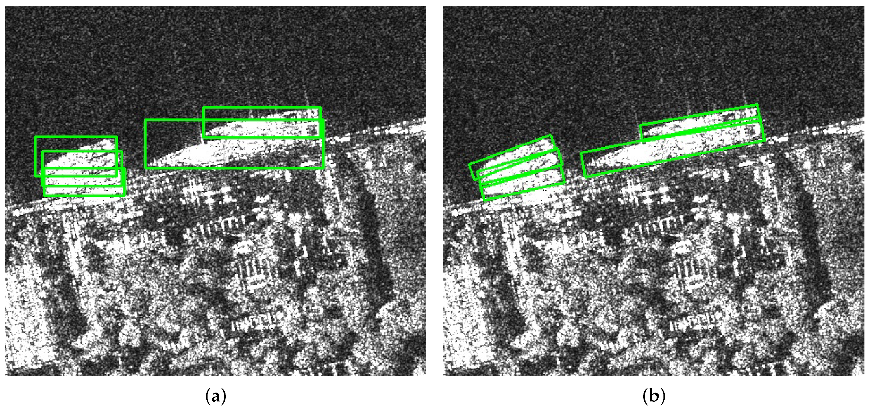Due to their slender shapes and arbitrary orientations, detecting ships using HBBs often results in significant inclusion of irrelevant background and adjacent targets, as shown in Figure 1a. In contrast, oriented bounding boxes (OBBs) are more appropriate for representing ship targets, as depicted in Figure 1b. However, generating OBBs is considerably more complex than HBBs due to the periodic rotation of OBBs, leading to issues of periodicity of angle (POA) and exchangeability of edge (EOE) [18,19,20]. As such, predicting OBBs with high accuracy poses a significant challenge. Previous works have employed additional branches [1,21] or complex techniques [18,19,22,23] to overcome the boundary problems associated with OBBs. However, such approaches result in significant network design complexity with limited gains in detection performance. Moreover, most existing methods suffer from redundant anchors [24,25,26,27] and feature misalignment problems [22,28,29], leading to inflexible and unwieldy designs.

To address the challenges associated with existing methods for SAR ship detection and leverage the latest advancements in deep learning, we propose a novel approach called KeyShip, an anchor-free key-point-based oriented detector for SAR ships. KeyShip simplifies the model design by removing predefined anchors and inefficient feature-aligning modules. It also introduces minor changes to the loss function to avoid boundary problems. Our work represents a new paradigm for detecting SAR ships with arbitrary orientations while achieving high accuracy.

Rather than relying on conventional box-based learning, we decompose each ship target into three distinctive parts: the long-edge center (LC), short-edge center (SC), and target center (TC). For each ship, there are two symmetrical parts for LC and SC and one center part for TC, for a total of five individual parts of three types. Although these ship parts may vary across images and ship targets under SAR imaging, they still contain the most common ship features. A CNN model is trained to generalize the diversified SAR features and localize these three types of parts as key points on three different heatmaps. By detecting ship parts, sufficient information can be collected to construct oriented bounding boxes while avoiding the uncertainty of direct oriented box learning. Compared with regression-based methods that require regressing the object’s border shape at a distance from the object’s center, the key points located at the boundaries of a target enable the network to describe the shape of ship targets with greater precision [30].

Traditional CNN-based key point detection networks [31,32,33] assign circular normalized two-dimensional (2-D) Gaussian blobs on heatmaps as the training targets. Considering the slender shape and size variance of ship targets, we propose to use shape-aware oriented elliptic 2-D Gaussian blobs as training targets for better performance.

Since scattered key points alone are insufficient for object detection tasks, subsequent key point clustering and oriented bounding box (OBB) reconstruction are required. To support the clustering of scattered key points, we propose a shape descriptor composed of the four pointers from the TC of an OBB to its four edge key points (SCs and LCs). However, as the SCs and LCs of a target are symmetric, a boundary problem arises if a fixed rule is used to assign the edge points to the TC for shape descriptor training. To alleviate this problem, we propose a soft edge point assignment strategy. During training, the geometric relationship between the LCs, SCs, and TC is learned explicitly, enabling the shape descriptor to provide a geometric clue for key point clustering and false alarm erasing.

At test-time, we propose a pipeline to cluster the scattered key points using the shape descriptors and construct oriented bounding boxes based on the clustered key points. However, due to the unreliability of long-range regression and the potential boundary problem, the shape descriptors do not always point to the exact location of the SCs or LCs. Random false alarms may also appear near the key points. To solve these problems, we propose a post-processing method called Gaussian reweighting based on the distance between the pointed positions of the shape descriptors and the candidate key points. Finally, we construct the oriented bounding box using the pair of SCs as the major axis of the box and the pair of LCs as the shorter axis. We provide the code for our approach at https://github.com/SlytherinGe/KeyShip.

In summary, our contributions are three-fold:

• We introduce an approach to represent an oriented SAR ship with three types of key points rather than an oriented bounding box. These key points resemble three typical positions of a SAR ship and are extended as shape-aware Gaussian blobs to train the detection model.
• We propose a shape descriptor to cluster the scattered key points detected on the heatmaps. The shape descriptor is trained with a soft edge point assignment strategy, which captures the geometric relationship between the key points and supports subsequent clustering.
• We present a compute-efficient pipeline to generate oriented bounding boxes from the detected key points at test time. Our pipeline uses a Gaussian reweighting technique to select key points and refine their positions, resulting in accurate and reliable bounding boxes.

2. Related Works

Object detection is a rapidly developing visual task with the aid of deep convolutional neural networks (CNNs). State-of-the-art (SOTA) object detection methods for natural images can be roughly divided into two categories: anchor-based detectors and anchor-free detectors.

Anchor-based methods—Anchor-based methods place predefined anchor boxes of different sizes and aspect ratios at every feature cell. They then regress the relative offsets based on the anchors to form bounding boxes and predict classification scores for each bounding box. Anchor-based detectors can be further divided into one-stage detectors [34,35,36] and two-stage detectors [37,38,39], each with relative advantages and limitations.

Anchor-free methods—Anchor-free methods are free of complicated anchor design and capable of producing comparable detection results. Vanilla anchor-free detectors regress the shape of the bounding box directly from each feature map cell and classify the generated box simultaneously. Representative methods of such include YOLO [40], FCOS [41] and RepPoints [42]. A trending branch of anchor-free detectors utilizes key points on heatmaps to detect individual targets. Methods such as CornerNet [31] and ExtremeNet [43] disassemble each target into separate parts and use key points to represent the object parts. By detecting the key points on heatmaps and grouping the key points from each target, such methods can directly align the object parts with feature maps and learn the spatial geometry of the objects, thus generating more precise bounding boxes compared with ordinary anchor-free methods [30].

To avoid the high complexity and low generalization capability of anchor design, our proposed method embraces key-point-based methods to simplify the model architecture while maintaining high performance and aligning target features at the object part level.

OBB-based detection—CNN-based object detection models commonly detect objects as horizontal bounding boxes (HBBs). However, the slender ship targets in SAR images can appear in any orientation, necessitating OBB-based detection methods.

Previous works on OBB-based detection can be viewed as extensions of HBB-based methods since many of them inherit the HBB-based detection design and obtain OBB results by adding an angle attribute. For example, RRPN [27] places multiple anchors of different scales, ratios, and orientations over each feature cell to generate proposals. Faster-RCNN-OBB [44] follows the pipeline of vanilla Faster-RCNN [37] but replaces the original corner-point representation of HBB with a four-vertex representation of OBB. ROITransformer [25] transforms horizontal region-of-interest (ROI) proposals into oriented proposals using relative offsets based on a local coordinate system. Oriented RCNN [24] regresses two offsets relative to the midpoints of the top and right sides of the anchor to form oriented proposals directly. Gliding Vertex [45] first predicts an HBB enclosing the target OBB from the previous horizontal proposal and then regresses the distances of the OBB’s four vertices relative to the enclosing HBB. Box Boundary-aware Vectors (BBAV) [21] represents the target OBB with four vectors in the four quadrants of the Cartesian coordinate system, allowing it to regress OBB targets directly.

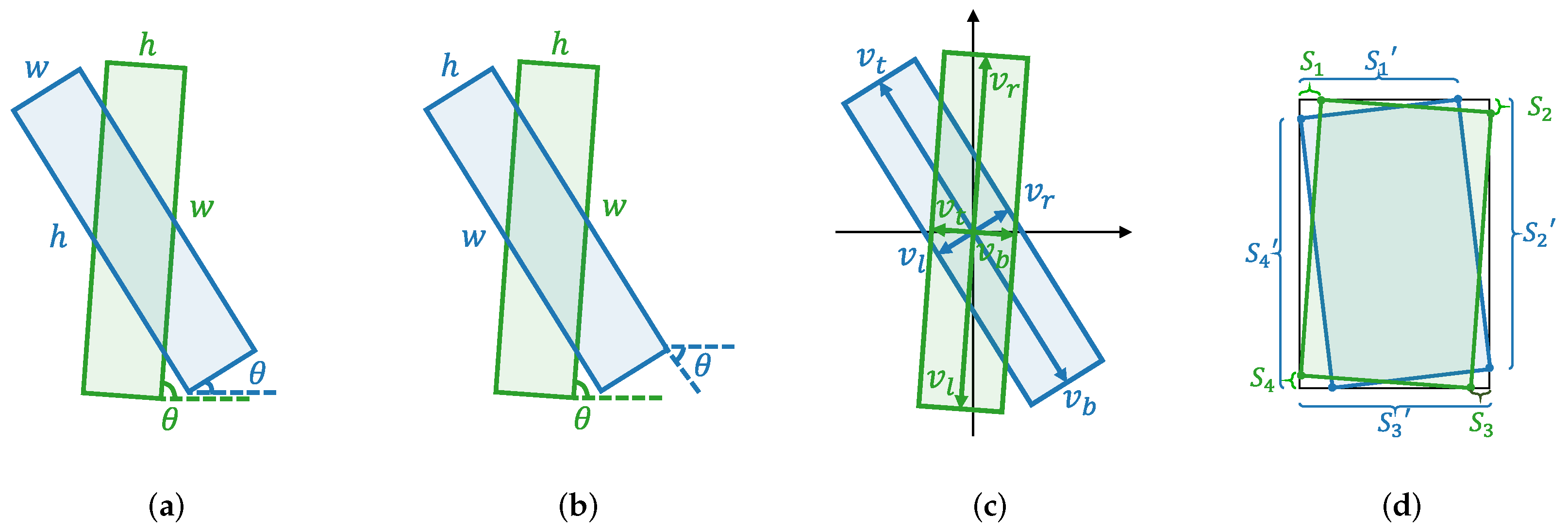
The boundary problem—Representing an orientated target with a periodic angle or exchangeable edges using a rigid OBB definition encounters the boundary problem [18]. When trained directly with these definitions, even if the predicted bounding boxes are highly overlapped with the ground truths, unreasonable losses may be produced due to the rigid training targets. Four commonly used definitions to describe OBBs and train detectors are illustrated in Figure 2. For a more detailed explanation of the boundary problem, please refer to [18,20].

Several methods have been proposed to handle the boundary problem. CSL [19] transfers the task of angle regression to classification to avoid ambiguity, while GWD [18] models each OBB as a two-dimensional Gaussian distribution and proposes a Gaussian Wasserstein distance regression loss to guide the learning of the distribution. To address the boundary problem, both [21,45] utilize extra branches to classify boundary cases and treat them as HBBs. Our method defuses periodic OBBs into non-periodic parts. We propose a shape descriptor to model a ship target as a combination of three types of key points and a specialized training target assignment strategy to alleviate the potential boundary problem in shape descriptor learning.

Ship detection—In the early stages, SAR ship detection was dominated by the Constant False Alarm Rate (CFAR) [47] detection algorithm and its subsequent modifications [48,49,50]. Apart from the CFAR-based methods, handcrafted features [51] and complex signals of SAR data [52] were also investigated for SAR ship detection. Many deep-learning-based methods have emerged recently. For instance, the study in [53] denoted each SAR ship as strong scattering points, then detected and grouped individual points to form the detection results. In [1], the shape of SAR ships was considered, and oriented Gaussian was used to train an improved Box Boundary-aware Vectors (BBAV). Polar encoding [20] placed vectors evenly distributed in polar coordinates to approximate the shape of the SAR ships. The study in [54] utilized the features from the strong scattering of SAR ships to aid the detection.

In optical images, CR2A-Net [28] proposed using a cascade detection head to refine misaligned features, achieving high-precision performance. The study in [55] improved RetinaNet by introducing a feature refinement module and using an IOU factor in the loss function to address the boundary problem. SKNet [56] regarded each ship as a center key point and proposed a soft NMS for post-processing. CHPDet [57] further encoded both the center and head of a ship as key points for detection.

Our work differs from some of the previous methods that manually integrate SAR features. Instead, we propose to utilize the full potential of the deep learning network in terms of feature learning. Our approach enables the network to learn the diverse SAR scattering into a set of virtual key points, thus detecting the ships with high precision.

3. Methods

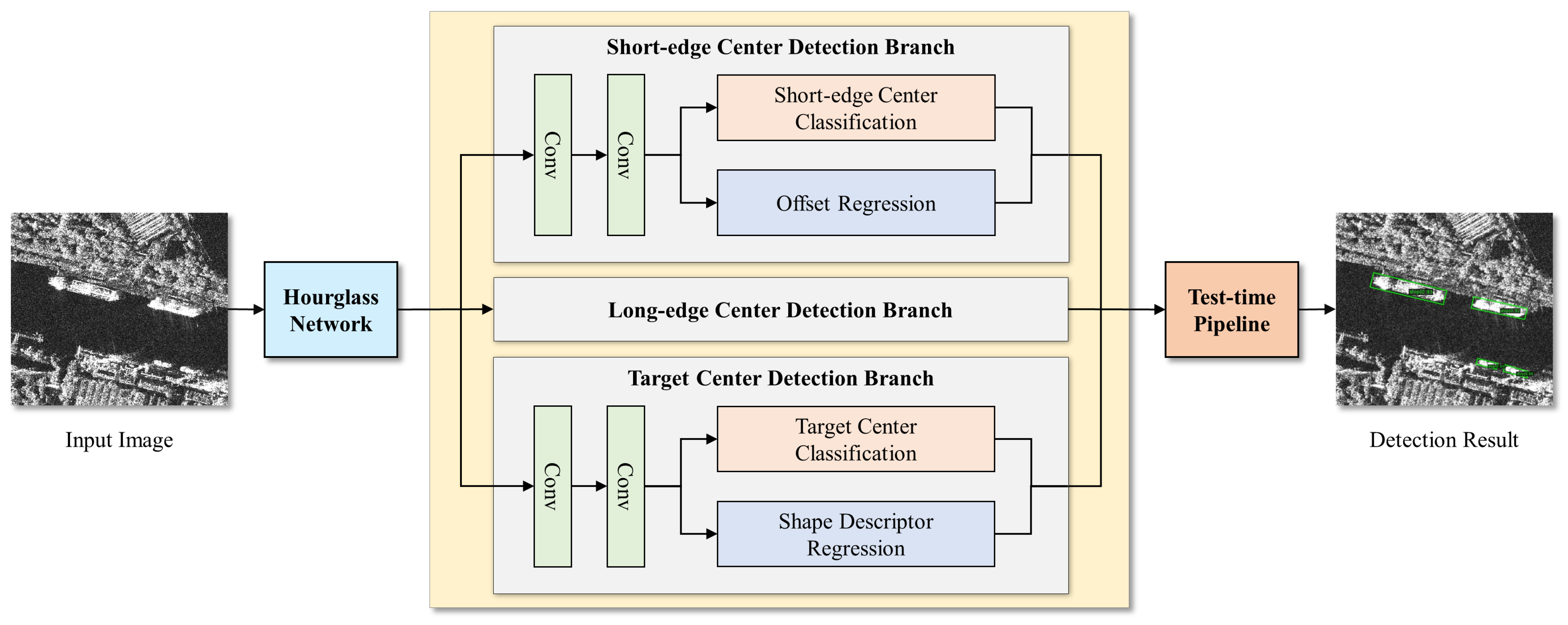
An overview of the proposed KeyShip detection method is depicted in Figure 3. The method starts with the input SAR image, which is processed using an Hourglass network [58] to extract high-level features. Then, the image features are passed through three parallel branches, each dedicated to detecting a specific type of key point. The long-edge and short-edge center detection branches are responsible for detecting the key points at the long-edge and short-edge centers of the targets, respectively, and predicting their corresponding offsets. The target center detection branch predicts the targets’ centers and the shape descriptors. A unique pipeline is utilized during the testing phase to cluster the key points and generate oriented detection results.

3.1. Key Point Classification

Ship targets in SAR images often have arbitrary orientations. An oriented target can be described by a five-parameter OBB $(x,y,w,h,\theta )$, in which $(x,y)$ is the position of the center, w and h are the lengths of the long and short edges, respectively, and $\theta$ is the rotation angle defined as, for example, the angle measured counter-clockwise between the long edge and the positive x-axis using the long-edge-based definition [19,27]. However, as aforementioned, it is difficult to regress these parameters with high accuracy in a single run. In this work, we propose a key-point-based method to describe oriented ships following the idea of ExtremeNet [43].

As illustrated in Figure 4a, we define three types of key points to describe a SAR ship target. The SCs and LCs are defined as the middle points at the short and long edges of an OBB, respectively. They are used to characterize the shape information of a target. The TC is defined as the center of the OBB and plays the role of objectness. The positions of these key points provide sufficient information to reconstruct the OBB. During training, the OBB annotations are used to form the key point representation for ship targets according to the previous definitions. We design three parallel branches for learning these key points, and each branch is assigned to detect a specific type of key point.

In this work, the key points are detected in a fully supervised classification manner, similar to the traditional keypoint-based object detection networks [31,32,33,43]. Given a heatmap $\widehat{\mathit{Y}}\in {(0,1)}^{H\times W}$ with height H and width W, which is designed to detect a specific type of key point (SCs, LCs, or TCs), we train it by using a target heatmap $\mathit{Y}\in {(0,1)}^{H\times W}$ with multiple Gaussian peaks, where each peak corresponds to a key point located at the corresponding cell of the heatmap. By training the network with this target heatmap $\mathit{Y}$, the resulting heatmap $\widehat{\mathit{Y}}$ will have a higher activation response around the key points and a lower response in the background area. The activation response of each cell in the heatmap can be interpreted as a confidence score of that cell being a key point.

However, in traditional methods, circular Gaussian blobs are used to generate the target heatmap $\mathit{Y}$ by using a 2-D Gaussian function with the same variance along the x-axis and y-axis. This approach has a critical flaw when dealing with a target with a slender body and an arbitrary orientation. To prevent background cells from being activated in the heatmap, the variance of the Gaussian function must be small, which restricts the energy of the Gaussian function within a limited portion of the target. This can make it difficult for the heatmap to activate on positions beneficial for key point detection. To overcome this issue, we propose to use shape-aware oriented Gaussian distributions as the training targets.

A 2-D Gaussian function with two standard deviations is capable of generating a Gaussian blob that has different distribution along the x-axis and y-axis, which is defined as

$$g(x,y)=exp\left(-\left(\frac{x^2}{2{{\sigma }_x}^2}+\frac{y^2}{2{{\sigma }_y}^2}\right)\right),$$

(1)

where ${\sigma }_x$ and ${\sigma }_y$ are the standard deviations along the x-axis and y-axis, respectively.

To account for the shape of the objects in the images, we define ${\sigma }_x$ and ${\sigma }_y$ relative to the object’s width and height, respectively. This ensures that the sizes of Gaussian blobs can change dynamically according to the size variances of the object annotations. Specifically, we define ${\sigma }_x$ and ${\sigma }_y$ as:

$$\begin{array}{cc}\hfill {\sigma }_x& ={\rho }_{w}w,\hfill \\ \hfill {\sigma }_y& ={\rho }_{h}h,\hfill \end{array}$$

(2)

where w and h are the width and height of the object’s oriented bounding box (OBB), and ${\rho }_w$ and ${\rho }_h$ are constant hyperparameters.

To generate the shape-aware oriented Gaussian distributions, we rotate the Gaussian blob generated by Equation (1) about its center by $\theta$ counter-clockwise, where $\theta$ is the angle of the object’s OBB. We then duplicate the rotated Gaussian blob at the positions of the specific key points (SCs, LCs, and TCs) on the training target $\mathit{Y}$, as shown in Figure 4b–d.

The imbalance between the number of key points on a heatmap and the background cells creates a significant challenge during training, with many more negative samples than positive samples. To address this issue, we adopt a modified version of the focal loss [35] as implemented in ExtremeNet [43]. The heatmaps of three different types of key points share the same loss function as

$$\begin{array}{c}\hfill L_{\det }=-\frac{1}{N}\sum _{i\in H\times W}\left\{\begin{array}{cc}{(1-\widehat{y_i})}^{\alpha }log\left(\widehat{y_i}\right),\hfill & \mathrm{if}{y}_i=1,\hfill \\ {(1-y_i)}^{\beta }{\widehat{y_i}}^{\alpha }log(1-\widehat{y_i}),\hfill & \mathrm{otherwise},\hfill \end{array}\right.\end{array}$$

(3)

where $\widehat{y_i}$ and $y_i$ are cell values on the predicted heatmap $\widehat{\mathit{Y}}$ and the training target $\mathit{Y}$, respectively. The $(1-y_i)$ term serves as a penalty to the loss function for the points around the positive samples, and $\beta$ controls the intensity of the penalty. $\alpha$ is a factor that emphasizes the hard examples, as in focal loss.

3.2. Offset Regression for SCs and LCs

Heatmaps are downsampled from the original images to detect key points, which can result in a loss of spatial precision. To address this issue, we added an offset regression module to each SC and LC detection branch, as shown in Figure 3. This module is similar to previous key point detection methods [1,31,43], which is implemented with a single $3\times 3$ convolution layer and outputs an offset map $\mathit{O}\in {\mathbb{R}}^{2\times W\times H}$, except that we train not only the key points but also the points around. By training the points around a key point to regress the offset of the key point, we get the opportunity to correct the errors when the points around the ground truth are detected as key points.

The loss for the offset regression module is defined as

$$L_{\mathrm{off}}=\frac{1}{M}\sum _k^N\sum _{i\in \mathcal{N}\left(k\right)}{\mathcal{L}}_{\mathrm{reg}}\left({\Delta }_i,\frac{{\mathit{x}}_k}{s}-{\mathit{x}}_i\right),$$

(4)

where N is the total number of ground truth SCs or LCs in the corresponding branch. $\mathcal{N}\left(k\right)$ is the set of samples selected to train for the k-th key point. In this work, the points around a key point whose Gaussian target is greater than a threshold ${\lambda }_1$, which is set to $0.5$ by default, are selected to train the module. M is the total number of training samples involved in offset regression. ${\Delta }_i$ is the predicted offset of the i-th sample in $\mathcal{N}\left(k\right)$. ${\mathit{x}}_k$ is the ground truth location of the k-th key point on the original image space and s is the downsampling scale of the heatmap. ${\mathit{x}}_i$ denotes the i-th sample’s location on the heatmap. ${\mathcal{L}}_{reg}$ can be any regression loss and the smooth $L1$ loss is used in this work.

3.3. Shape Descriptor Regression

We propose a shape descriptor that supports the clustering process to construct OBBs from the scattered key points detected on heatmaps. The BBAV approach [21] assigns four vectors to the center of an OBB and trains the vectors to point to its borders in the four quadrants according to a fixed strategy. Similarly, we assign four pointers to the TC and train the pointers to point to the corresponding SCs and LCs, but with a dynamic training strategy. 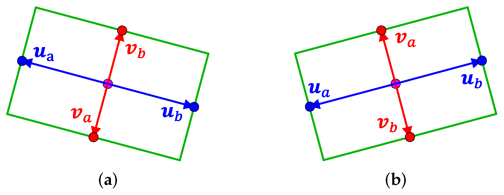The dynamic training strategy can elegantly elevate the boundary problem, so we do not have to predict extra parameters such as box width $w_e$, box height $h_e$, and orientation indicator $\alpha$ like BBAV to handle cases where bounding boxes are horizontal, which is the key difference between our proposed shape descriptor and BBAV. By avoiding the need to predict these extra parameters, our method reduces the overall complexity of the model and results in a more efficient and accurate approach for detecting objects with varying orientations. As illustrated in Figure 5a, a shape descriptor consists of four pointers that start from the TC and extend to the edge key points, each described by an offset vector starting from the TC. Specifically, the pointers to the SCs are denoted as ${\mathit{u}}_a$ and ${\mathit{u}}_b$, and those to the LCs as ${\mathit{v}}_a$ and ${\mathit{v}}_b$. A shape descriptor can be formulated as an eight-parameter vector by concatenating the four pointers:

$$\mathit{p}=\left[{\mathit{u}}_a,{\mathit{u}}_b,{\mathit{v}}_a,{\mathit{v}}_b\right].$$

(5)

The shape descriptor regression module in KeyShip is implemented with a single $3\times 3$ convolution layer, which outputs a heatmap $\mathit{P}\in {\mathbb{R}}^{8\times W\times H}$ of the shape descriptors according to the upstream TC features.

To train the shape descriptor regression module, specific rules are required to associate the pointers of shape descriptors with the SC and LC key points, which serve as the training targets. As shown in Figure 5, the SC on the left of TC is assigned to pointer ${\mathit{u}}_a$, while the SC on the right is assigned to ${\mathit{u}}_b$, and the same rule applies to the LC pointers ${\mathit{v}}_a$ and ${\mathit{v}}_b$. This method of assigning training targets for the shape descriptors based on the relative positional relationship between key points can be regarded as a prototypical fixed edge point assignment strategy. However, this fixed strategy may cause difficulties in training the shape descriptor. When the boundary problem arises, as illustrated in Figure 5b, the association of ${\mathit{v}}_a$ and ${\mathit{v}}_b$ with the LC key points is opposite to that in Figure 5a due to the difference in orientation of the two OBBs. The exchange of the two pointers between two similar OBBs in Figure 5 reveals a typical scenario of the boundary problem. This problem leads to misleading training of ${\mathit{v}}_a$ and ${\mathit{v}}_b$ pointers using similar features on the sides of ship targets. The same problem also occurs with ${\mathit{u}}_a$ and ${\mathit{u}}_b$ pointers for nearly vertical OBBs. If the boundary problem is not properly solved, shape descriptors of poor quality for the targets in horizontal or vertical orientation will be produced. In Section 4.5, we visualized some typical false cases for the shape descriptors in a real test image when the boundary problem arises, please refer to it for more details.

In this work, we propose a soft edge point assignment strategy to alleviate the boundary problem. Our motivation is based on the observation that irrespective of how the key point assignment strategy is defined, there are a total of four different shape descriptor representations for an OBB, as shown in Figure 6. Our soft assignment approach aims to select the most suitable shape descriptor by comparing the predicted pointers with all four possible association scenarios rather than strictly adhering to a predetermined rule. We achieve this by using a shape descriptor loss, denoted as $L_{\mathrm{sd}}$, which is defined as follows:

$$L_{\mathrm{sd}}=\frac{1}{M}\sum _k^N\sum _{i\in \mathcal{N}\left(k\right)}{l}_i,$$

(6)

where N denotes the total number of ground truth TCs, and $\mathcal{N}\left(k\right)$ represents the set of samples chosen to train for the k-th TC. The training samples are selected as the points around a TC whose Gaussian target is greater than the threshold ${\lambda }_2$, which is set to 0.5 by default. The total number of training samples is denoted as M. The loss for the i-th sample in $\mathcal{N}\left(k\right)$, denoted by $l_i$, is calculated using the following formula:

$$\begin{array}{cc}\hfill l_i=min& \left({\mathcal{L}}_{reg}({\mathit{u}}_{ai},{\widehat{\mathit{u}}}_{ai})+{\mathcal{L}}_{reg}({\mathit{u}}_{bi},{\widehat{\mathit{u}}}_{bi}),{\mathcal{L}}_{reg}({\mathit{u}}_{ai},{\widehat{\mathit{u}}}_{bi})+{\mathcal{L}}_{reg}({\mathit{u}}_{bi},{\widehat{\mathit{u}}}_{ai})\right)+\hfill \\ \hfill min& \left({\mathcal{L}}_{reg}({\mathit{v}}_{ai},{\widehat{\mathit{v}}}_{ai})+{\mathcal{L}}_{reg}({\mathit{v}}_{bi},{\widehat{\mathit{v}}}_{bi}),{\mathcal{L}}_{reg}({\mathit{v}}_{ai},{\widehat{\mathit{v}}}_{bi})+{\mathcal{L}}_{reg}({\mathit{v}}_{bi},{\widehat{\mathit{v}}}_{ai})\right).\hfill \end{array}$$

(7)

where ${\widehat{\mathit{u}}}_{ai}$, ${\widehat{\mathit{u}}}_{bi}$, ${\widehat{\mathit{v}}}_{ai}$ and ${\widehat{\mathit{v}}}_{bi}$ are the predicted pointers for the i-th sample, and ${\mathit{u}}_{ai}$, ${\mathit{u}}_{bi}$, ${\mathit{v}}_{ai}$ and ${\mathit{v}}_{bi}$ are the ground truth pointers at the corresponding sample. ${\mathcal{L}}_{reg}$ is the same as in Equation (4). In other words, $l_i$ evaluates the model’s predictions with respect to all four possible shape descriptors using the metrics $L_{reg}$. It then selects the most suitable shape descriptor as the training target by identifying the one that best resembles the model output, and calculates the loss between them.

3.4. Test-Time Pipeline

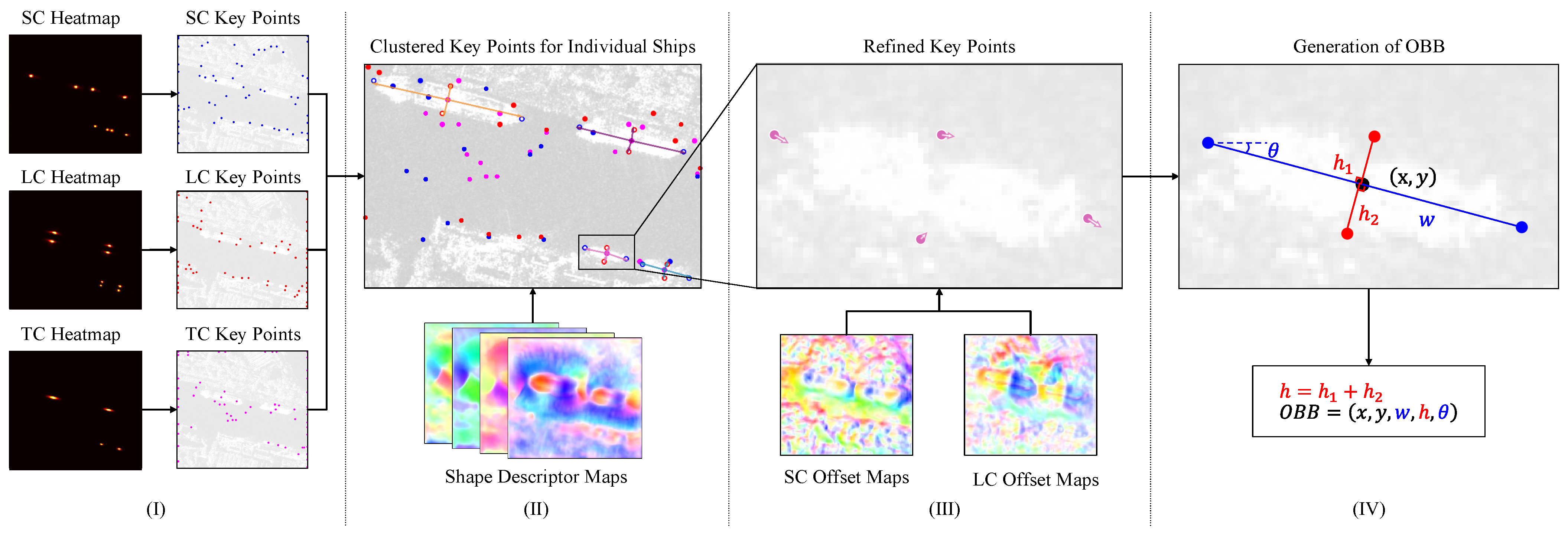
To construct the OBB detection results, we propose a test-time pipeline for aggregating the six heatmaps output by the three branches in KeyShip. The pipeline consists of four processes, denoted as step I to IV, as illustrated in Figure 7.

(I)

Key Point Detection

The key points are detected separately on the three classification heatmaps. First, the center points with the highest scores in the $3\times 3$ regions on a heatmap are selected as candidates. Then, the top K points with the highest scores among the candidates are regarded as the key points for further processing. A group of detection results is shown in Figure 7I, where the blue, red and purple dots represent the detected SC, LC and TC key points, respectively.

(II)

Key Point Clustering

The detected TC key points’ corresponding shape descriptors can be obtained from the heatmap for shape descriptor regression. We use the shape descriptors to find the edge key points associated with the TC key points, thus achieving the clustering of the scattered key points. However, due to the inconsistency between the shape descriptor regression and the key point detection tasks, the pointers in the shape descriptors may not point at the exact locations of the detected SC and LC key points. Multiple key edge points may pack around the pointed locations, some of which are false alarms, while others are the key points for other targets. We introduce a Gaussian reweighting technique to associate the most appropriate edge key point with each pointer of a shape descriptor.

First, we associate the SC and LC key points with the SC and LC pointers of the shape descriptors, respectively. For instance, let $\{{\mathit{o}}_k,k=1,\cdots ,K\}$ be the detected TC key points and $\{{\mathit{x}}_j,j=1,\cdots ,K\}$ be the detected SC key points. Since each shape descriptor has two SC pointers, we denote the endpoints of the SC pointers of the shape descriptors at the detected TCs as $\{{\mathit{z}}_i,i=1,\cdots ,2K\}$. We define the relevance score between ${\mathit{z}}_i$ and ${\mathit{x}}_j$ as follows:

$$r({\mathit{z}}_i,{\mathit{x}}_j)=S_{SC}\left({\mathit{x}}_j\right)·exp\left(-\frac{d{\left({\mathit{z}}_i,{\mathit{x}}_j\right)}^2}{2{\sigma }^2}\right),$$

(8)

where the function $S_{SC}(·)$ outputs the confidence score at the input point from the SC classification heatmap and the function $d(·,·)$ calculates the Euclidean distance between the two inputs. $\sigma$ is a hyperparameter to control the penalty for the distant key points and is set to $0.01$ by default. The SC key point associated with ${\mathit{z}}_i$ and its confidence score can be determined by

$$\begin{array}{c}\hfill \mathcal{K}\left({\mathit{z}}_i\right)=\left\{\begin{array}{cc}arg\underset{{\mathit{x}}_j}{max}r({\mathit{z}}_i,{\mathit{x}}_j),\hfill & r({\mathit{z}}_i,{\mathit{x}}_j)>t,\hfill \\ {\mathit{z}}_i,\hfill & \mathrm{otherwise},\hfill \end{array}\right.\end{array}$$

(9)

$$\begin{array}{c}\hfill S\left({\mathit{z}}_i\right)=\left\{\begin{array}{cc}\underset{{\mathit{x}}_j}{max}r({\mathit{z}}_i,{\mathit{x}}_j),\hfill & r({\mathit{z}}_i,{\mathit{x}}_j)>t,\hfill \\ t,\hfill & \mathrm{otherwise},\hfill \end{array}\right.\end{array}$$

(10)

where $\mathcal{K}(·)$ functions to assign a key point for the input pointer based on the relevance score between them. If the relevance score between the input pointer and a key point is greater than the threshold t, the key point with the highest relevance score is assigned. Otherwise, the endpoint of the pointer is used as the key point. $S(·)$ returns the relevance score of the selected key point as the confidence score for further process. The threshold t is set to $0.01$ by default to prevent distant key points from being matched to the pointer. This scheme allows the pointer to generate a key point at its pointed location if no valid key points are available, compensating for the miss detection of key points by utilizing the shape information of the shape descriptor.

After the detected SC and LC key points are associated with the shape descriptors, we define the confidence score of a target detected at the TC position ${\mathit{o}}_k$ as

$$S_{tgt}\left({\mathit{o}}_k\right)=\frac{2·S_{TC}\left({\mathit{o}}_k\right)+{\sum }_{\mathit{z}\in p\left({\mathit{o}}_k\right)}S\left(\mathit{z}\right)}{6},$$

(11)

where $S_{TC}(·)$ outputs the confidence score at the input point from the TC classification heatmap and $p\left({\mathit{o}}_k\right)$ is a set of the endpoints of the shape descriptor at ${\mathit{o}}_k$. The score reflects both the target objectness and the quality of its component detection. By thresholding the score, we can also determine the endurance of the miss detection of ship parts, thus balancing between the precision and recall of the detection result.

The process of the key point clustering is illustrated in Figure 7II. Different colors are used to render the shape descriptors for different target instances. The shape descriptors that fail to form the final results are not visualized. White dots are placed at the center of the key points associated with the shape descriptors.

(III)

Refinement of Key Points

In this step, the positions of the SC and LC key points that are successfully clustered are refined by adding offsets sampled from the offset maps of the SC and LC branches, respectively. The refining process is illustrated in Figure 7 as step III. The four circles in the same color are the SCs and LCs clustered for the enlarged ship target, and the orientation and length of the arrows represent the offsets’ orientation and length for refinement.

(IV)

OBB Generation

In this step, the OBBs are constructed based on the clustered key points. We utilize the long-edge definition [19,27], namely defining the long-edge of the target as width and the angle between the long-edge and the x-axis as the orientation angle, to encode the ship targets. Considering that the TC key points are not refined in this work, the average position of the refined SC and LC key points is used as the center of the OBB. The width and the orientation angle are defined by the line segment between the two refined SCs. The height is obtained by summing the distances from the refined LCs to the line segment between the two refined SCs. The considerations of such designs are as follows. During the test time, the detected SCs are more likely to fall in the exact center of the edges than the LCs, which is why we use the SC line segment and the perpendicular lines from LCs to form the width and height of an OBB, respectively, for better accuracy. Furthermore, for the same degree of the positional shift of the key points, using SCs to determine the orientation of an OBB will also introduce less turbulence into the OBB orientation as the SC line segment is longer than that of the LCs. The whole encoding process is illustrated in Figure 7 as step IV.

4. Results

4.1. Datasets and Evaluation Metrics

We conducted experiments on two public SAR ship detection datasets, SSDD [2] and RSDD [3], to evaluate the proposed method. Both two datasets only contain SAR images for benchmarking the methods for the SAR ship detection task. Additionally, we evaluated the proposed method on an optical ship detection dataset called HRSC2016 [59] to further validate its robustness.

SSDD includes 1160 image chips in total, 928 for training and 232 for testing. It provides three types of annotations, namely HBB, OBB and instance segmentation annotations. The images are taken from RadarSet-2, TerraSAR-X and Sentinel-1 with resolutions ranging from 1 to 15 m, with image sizes ranging from 214 to 668 pixels in width and 160 to 526 pixels in height. Four polarization modes, HH, VV, HV and VH, are contained in the dataset. Following the guidance of the official release, 232 images with indexes ending in 1 and 9 were selected for testing and the other 928 images were used for training. All images were resized and padded to the size of $640\times 640$ and augmented with techniques such as random flipping to prevent overfitting during training.

RSDD is a newly released SAR ship detection dataset with OBB annotations, comprising 7000 image chips. The images are taken from Gaofen-3 and TerraSAR-X with resolutions ranging from 2 to 20 m. Polarization modes of HH, HV, VH, VV, DV and DH are contained in this dataset. The images are $512\times 512$ chips cropped from the large-scene raw images. The dataset was randomly divided into two parts, a training set and a testing set, with 5000 and 2000 images, respectively. All images were resized to $640\times 640$ and data augmentation techniques were applied to the training set.

HRSC2016 is a high-resolution ship detection dataset based on optical satellite images. The image sizes range from $300\times 300$ to $1500\times 900$. This dataset contains 436 images for training, 181 for validation, and 444 for testing. As the training set is too small, we combined all the images from the training and validation sets for training. All images were resized to $800\times 800$, and the same data augmentation techniques were applied as the other datasets.

We adopted average precision (AP) as the evaluation metric in our experiments, which is the same as the PASCAL VOC 2007 object detection challenge [60]. The AP is calculated as

$$AP=\frac{1}{11}\sum _{r\in \left\{0,0.1,\dots ,1\right\}}{P}_{interp}\left(r\right),$$

(12)

$$P_{interp}\left(r\right)=\underset{\tilde{r}:\tilde{r}\ge r}{max}p\left(\tilde{r}\right),$$

(13)

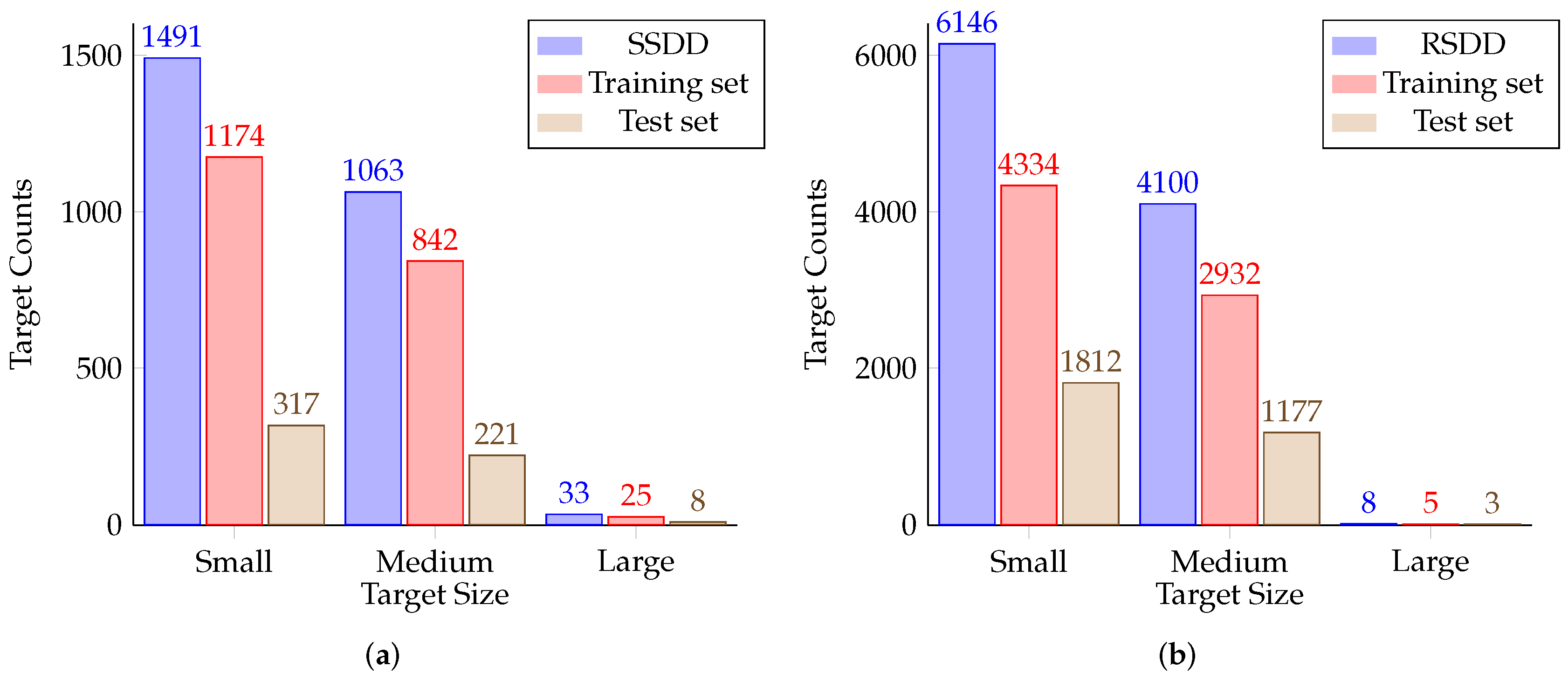
where r indicates the recall rate, which is a set of 11 levels evenly sampled from 0 to 1. $p\left(\tilde{r}\right)$ is the measured precision at recall $\tilde{r}$. We calculated the AP at 10 IOU thresholds ranging from 0.5 to 0.95 with a stride of 0.05. The average of the 10 APs was also computed to represent the overall performance, as in the COCO dataset [61]. In addition, we calculated the APs for small, medium and large targets to evaluate the performance of the methods concerning the target sizes in SSDD and RSDD datasets. Unlike the definition of small, medium and large targets in COCO, we adopted the classification criterion from [2] shown in

Table 1. Target size classification criterion.

Small	Medium	Large
Area < 625	625 ≤ Area ≤ 7500	Area > 7500

due to the difference between the HBB and OBB annotations. The size distributions of the two datasets are shown in Figure 8.

In the following, the AP at a specific IOU threshold is denoted as $APX$. For example, $AP50$ denotes the AP at the IOU threshold of 0.5. The AP for small, medium and large targets are denoted as $A{P}_s$, $A{P}_m$ and $A{P}_l$, respectively. The bare $AP$ indicates the mean of the ten $APX$ for simplicity.

In addition to AP, we also used the F1 score as another important index to reflect the overall performance of a method. The F1 score indicates the performance of a method under a single-point confidence threshold, and we take the maximum F1 from all thresholds for comparison. The F1 score can be calculated by

$$F1=\underset{r\in R}{max}\left(2·\frac{r·p\left(r\right)}{r+p\left(r\right)}\right)$$

(14)

where R represents all possible recall rates under different confidence thresholds given the detection results. We also evaluate F1 scores under different IOU thresholds like AP. In the following, $F1·50$ and $F1·75$ denote the F1 score under the IOU threshold 0.5 and 0.75, respectively.

4.2. Implementation Details

We used Hourglass104 [58] as the backbone network of the proposed method. To make a fair comparison, we chose ResNet101 [62] as the backbone network for the comparison methods. Experiments were carried out upon the Pytorch [63]-based benchmark toolbox MMRotate [64]. The weights of the ResNet101 were initialized with the pre-trained model on the ImageNet [65] dataset, while the weights of the Hourglass104 were initialized with a CentripetalNet [32] pre-trained on COCO [61] dataset because the Hourglass network cannot be pre-trained on ImageNet directly. At the end of each method, the non-maximum-suppression (NMS) algorithm was utilized to remove the duplicate OBBs. We adopted the Adam optimizer with an initial learning rate of $6\times {10}^{-4}$. The first 50 iterations of the training were used to warm up the learning rate. The learning rate was decayed by a factor of 10 at the 110th epoch, and the training stopped after the 150th epoch. The entire batch size was 4 on two Nvidia Titan V graphics cards with 12-G memory each. For the training of the comparison methods, the optimizer and the training schedule are slightly different from our proposed method. See Section 4.7 for more details.

4.3. Multitask Training

The training loss function of the proposed method is a sum of the weighted individual losses:

$$\begin{array}{c}\hfill L=\sum _{t\in \left\{\mathrm{TC},\mathrm{SC},\mathrm{LC}\right\}}\gamma L_{\det }^t+\sum _{t\in \left\{\mathrm{SC},\mathrm{LC}\right\}}\eta L_{\mathrm{off}}^t+\xi L_{\mathrm{sd}},\end{array}$$

(15)

where $\gamma$ is set to $1/3$ to balance the contributions of the losses from three heatmap classification branches. We set $\eta$ and $\xi$ to $0.1$ and $0.05$ to scale down the regression loss as they are numerically larger than the classification loss. As in previous works [31,32,43], we added intermediate supervision for the Hourglass104 Network.

4.4. Effectiveness of the Oriented Gaussian Training Targets

4.4.1. Hyperparameter Analysis

In this section, we analyze the impact of the hyperparameters ${\rho }_w$ and ${\rho }_h$ on the performance of the final detection results on SSDD. These hyperparameters control the proportion of a Gaussian blob that covers an OBB, thereby determining the generated shape-aware oriented Gaussian training targets.

To investigate the effect of these hyperparameters, we set ${\rho }_w$ and ${\rho }_h$ to the same value and increased them from 0.10 to 0.40 in step sizes of 0.05. The results are presented in

Table 2. Effect of Hyperparameters ${\rho }_w$ and ${\rho }_h$.

${\mathit{\rho }}_{\mathit{w}}$	${\mathit{\rho }}_{\mathit{h}}$	$\mathit{AP}$	$\mathit{AP}50$	$\mathit{AP}75$	$\mathit{AP}90$
0.10	0.10	0.5572	0.9068	0.5835	0.0726
0.15	0.15	0.5810	0.9056	0.6625	0.1056
0.20	0.20	0.5813	0.9043	0.6675	0.1129
0.25	0.25	0.5813	0.9072	0.6718	0.1126
0.30	0.30	0.5703	0.9062	0.6647	0.0820
0.35	0.35	0.5718	0.9077	0.6643	0.0572
0.40	0.40	0.5739	0.9056	0.6638	0.1042

. The $AP$ value initially increased with increasing values of ${\rho }_w$ and ${\rho }_h$, reaching a maximum of $0.5813$ at $0.20$ and $0.25$, before decreasing thereafter. These results suggest that the proper coverage of a Gaussian blob on an OBB is crucial to the final performance of the proposed method. If the Gaussian blobs are too small, many pixels within the OBBs are regarded as negative samples during training, making the key points poorly activated at test time, which could cause missing detection of key points and pose difficulty in the NMS stage. On the contrary, oversized Gaussian blobs corrupt the contributions of the true negatives around the key points during training, resulting in unexpected activation on the heatmaps during the test time.

In the following experiments, we set both ${\rho }_w$ and ${\rho }_h$ of the proposed method to $0.25$ for its balanced performance on different IOU levels.

4.4.2. Oriented versus Circular Gaussian Training Targets

In this section, we compare the advantage of the proposed shape-aware oriented Gaussian training targets with the normal circular Gaussian targets on SSDD. The variances of the circular Gaussian targets were set to $min\left({\sigma }_w,{\sigma }_h\right)$ to avoid undesired penalties outside the ship target. The ${\rho }_w$ and ${\rho }_h$ in both experiments were set to 0.25.

As shown in

Table 3. Effectiveness of Oriented Gaussian Training Targets.

Key Point Training Targets	$\mathit{AP}$	$\mathit{AP}50$	$\mathit{AP}75$	$\mathit{AP}90$
Circular Gaussian Targets	0.5569	0.9055	0.6593	0.1034
Proposed Gaussian Targets	0.5813	0.9072	0.6718	0.1126

, the KeyShip detector trained using circular Gaussian targets suffers from a performance drop due to the circular Gaussian blob’s poor capability of covering the slender oriented targets. This finding demonstrates the superiority of our proposed oriented Gaussian training targets.

4.5. Effectiveness of the Shape Descriptor and Soft Edge Point Assignment Strategy

4.5.1. Soft versus Fixed Edge Point Assignment

We experimented on SSDD to compare the proposed soft edge point assignment strategy with the fixed assigning strategy used in Figure 5. To focus the evaluation on the capabilities of the shape descriptor and the soft assignment strategy, we used a simplified KeyShip model that included only the target center branch. All operations related to the SC and LC branches, such as the SC and LC key point detection, key point clustering, and SC and LC key point refinement, were not performed during the test time. The OBBs were generated directly based on the detected TC key points and the shape descriptors.

Table 4. Effectiveness of the Shape Descriptor.

Target Assignment	$\mathit{AP}$	$\mathit{AP}50$	$\mathit{AP}75$	$\mathit{AP}90$
Fixed Strategy	0.4556	0.8097	0.4631	0.0227
Soft Strategy	0.4700	0.9017	0.4727	0.0315

shows that our shape descriptor alone produces satisfactory detection results, regardless of whether the fixed or soft assignment strategy is used. This suggests that the shape descriptor can be separated from our method and attached to any other detection backbone to form a new detector. When the soft edge point assignment strategy is applied, the $AP$ score is increased from $0.4556$ to $0.4700$, indicating that the soft assignment is beneficial in the presence of ambiguous training targets.

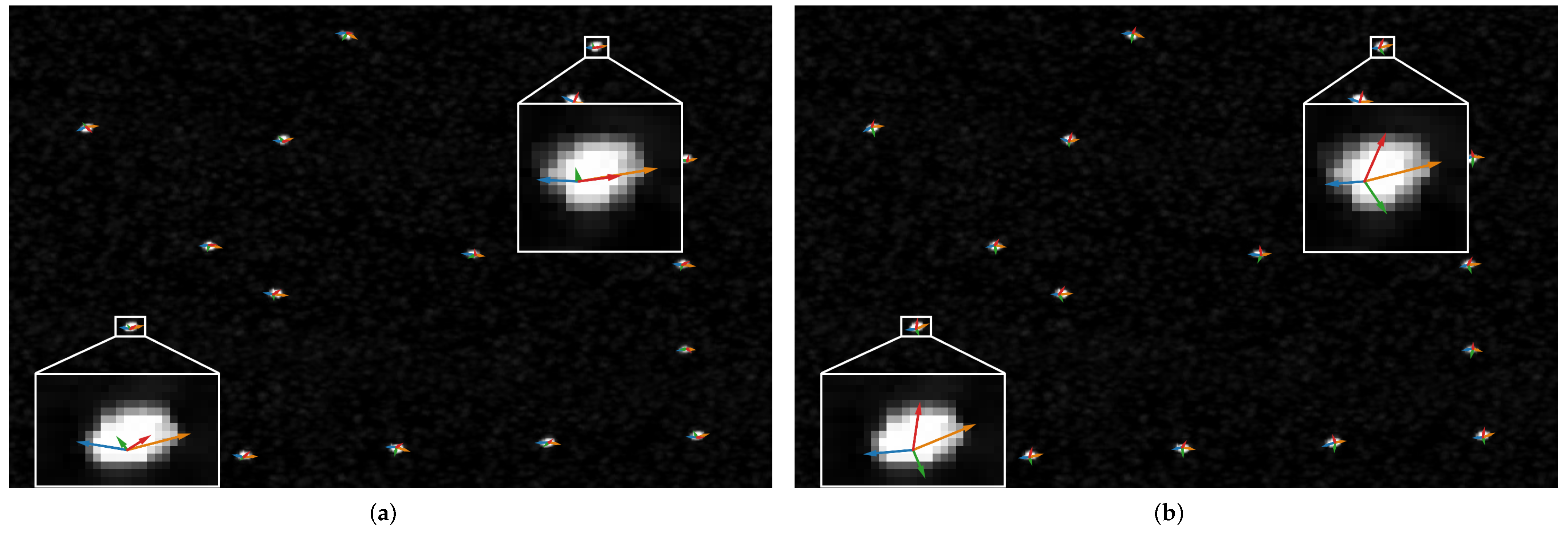
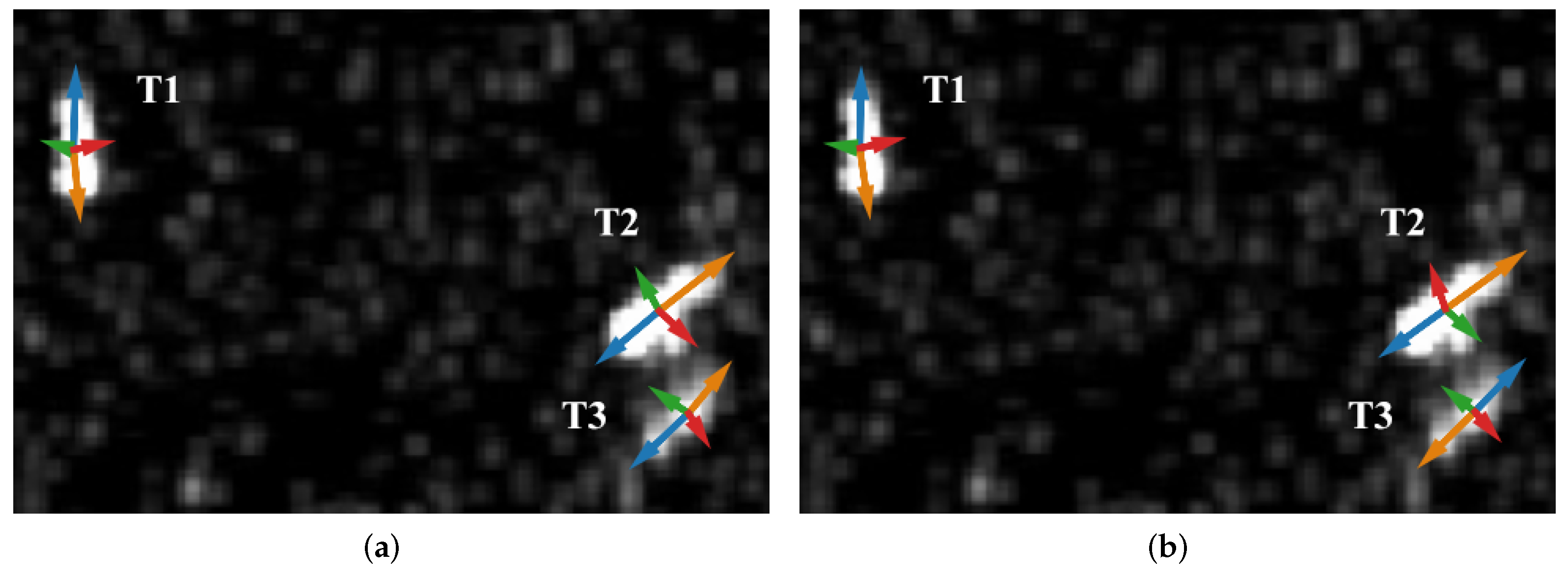
To better understand the reason for the performance improvement from the soft assignment strategy, we visualized the shape descriptors obtained on a test image in SSDD by the two assignment strategies in Figure 9. Following the formulation of Equation (11), shape descriptors whose corresponding target confidence scores fall below a threshold of 0.15 are automatically removed and are not visualized. Consequently, only those shape descriptors that contribute to the final oriented bounding box detection results are visualized. This thresholding protocol applies to both the visualizations presented in Figure 9 and Figure 10, ensuring that only relevant shape descriptors are included in the analysis. As shown in Figure 9a for the fixed assignment strategy, the LC pointers (i.e., the green and red pointers) of some targets mistakenly point at the upper border simultaneously, which is a typical manifestation of the boundary problem. We observed that the boundary problem arises when the target is relatively small, and the semantic features are weak. On the contrary, the shape descriptors trained by our soft assignment strategy in Figure 9b are free of the boundary problem and work perfectly in the case of failures in Figure 9a.

4.5.2. Additional Benefits of Soft Assignment Strategy in Addition to Improved Performance

Figure 10 visualizes the shape descriptors trained by the fixed and the soft assignment strategies on another test image in SSDD. It shows that both assignment strategies predict the shape descriptors of the three targets satisfactorily so that their final target detection results would not differ significantly. However, upon closer observation, we can conclude that the shape descriptors trained by the soft assignment strategy offer additional benefits beyond improved performance.

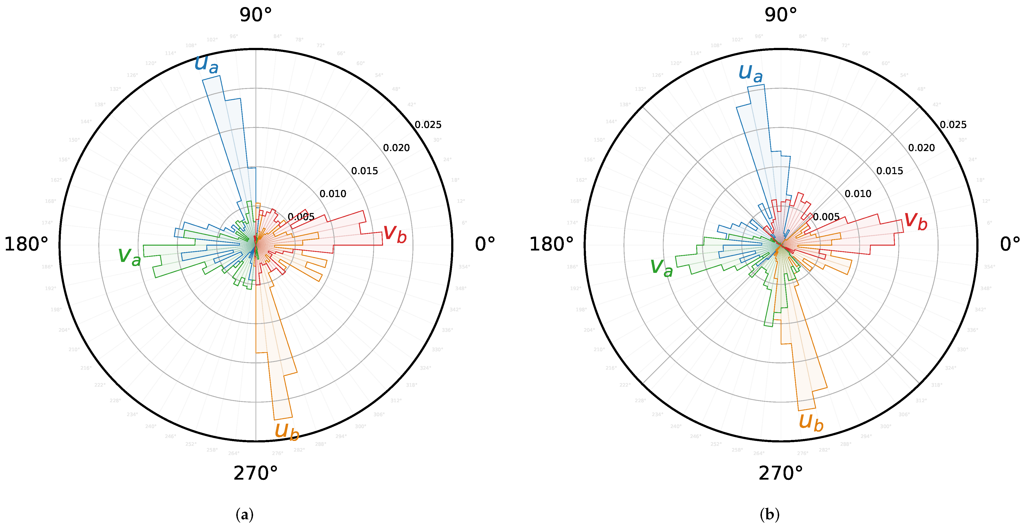
Specifically, the soft assignment strategy not only learns to point at the edge centers of the targets but also learns the geometric relationships between the individual pointers. This conclusion is supported by the histograms of the pointer orientations shown in Figure 11, which were counted based on all shape descriptors that yielded valid detection results on the test set of SSDD.

For ease of description and understanding, we use the colors of the pointers to refer to them. In Figure 10a, under the constraint of the fixed assignment strategy, the blue pointers (SC pointer $u_a$) and the green pointers (LC pointer $v_a$) always point to the left, while the orange pointers ($u_b$) and red pointers ($v_b$) always point to the right. This can be seen more clearly in Figure 11a. However, the spatial relationship between the SC and LC pointers is inconsistent for different targets. For example, in Figure 10a, for target T1, the blue pointer is clockwise ahead of the green pointer by about ${90}^{\circ }$, but it is behind the green pointer for T2 and T3. This inconsistency suggests that the fixed assignment strategy fails to learn a stable relationship between the pointers of a shape descriptor.

In contrast, the soft assignment strategy implicitly learns a stable relationship between the pointers of a shape descriptor. In Figure 10b, for all shape descriptors obtained by the soft assignment strategy, the four pointers form a consistent order, clockwise in blue, red, orange, and green. Figure 11b displays the histograms of the pointer orientations for the soft assignment strategy, where the blue and orange pointers are each distributed on one side of the ${45}^{\circ }$ diagonal, while the red and green pointers are each distributed on one side of the ${135}^{\circ }$ diagonal. This indicates that the soft assignment strategy automatically learns the optimal boundaries for the SC and LC pointers. Not only that, but it also implicitly learns the spatial relationship between different types of pointers, as described above.

In summary, the proposed soft edge point assignment strategy can implicitly learn a stable relationship between the pointers of a shape descriptor. It offers a flexible solution for the representation learning of a target with a periodic angle or exchangeable edges, and this feature might be beneficial to tasks requiring strong structure learning.

4.6. Ablation Study

In order to further evaluate the proposed method, we conducted an ablation study on the different components of the model using the SSDD dataset. Specifically, we investigated the effectiveness of the SC and LC key point detection in achieving high-accuracy SAR ship detection.

To do this, we compared the performance of three KeyShip models: a baseline model with only the TC branch, a full model design without offset regression and key point refinement, and a full model design. The results are shown in

Table 5. Ablation Study on SSDD.

Target Center Branch	SC & LC Key Point Detection	Offset Regression	$\mathit{AP}$	$\mathit{AP}50$	$\mathit{AP}75$	$\mathit{AP}90$
√			0.4700	0.9017	0.4727	0.0315
√	√		0.5340	0.9062	0.5501	0.0909
√	√	√	0.5813	0.9072	0.6718	0.1126

.

Our analysis indicates that while all three detectors have the ability to roughly determine whether a target is present at a given location, the precision of the baseline model is poor, as evidenced by the low $AP75$ and $AP90$ scores. This suggests that the objects can be detected by the target center branch alone, but the detection results lack precision.When the SC and LC key point detection are added to the baseline model, the values of $AP75$ and $AP90$ increase significantly. Furthermore, when the offset regression is applied, there is a noticeable improvement in the $AP$ and $AP75$ scores. This emphasizes the importance of local offset refinement in improving the accuracy of key point detection.

Overall, these experimental results reaffirm the difficulty in accurately describing the shape of an object using unaligned object features in the regression tasks and further highlight the significance of key point detection in achieving high-precision detection results.

4.7. Quantitative Comparison with SOTA Methods

To validate the superior detection accuracy of the proposed method compared to the state-of-the-art (SOTA) oriented object detection methods, we conducted comparative experiments on three datasets, SSDD, RSDD and HRSC2016. We selected several powerful and typical oriented object detectors, including Rotated RetinaNet [35], R3Det [22], GWD [18], S2ANet [29], Gliding Vertex [45], BBAV [21], Rotated Faster RCNN [37], Oriented RCNN [24], ROITransformer [25], and OrientedRepPoints [66]. Additionally, Polar Embedding [20], an oriented SAR ship detection method, was also benchmarked on the SSDD and RSDD datasets.

Experimental settings were carefully considered to ensure a fair comparison of the proposed method with the previous SOTA methods. The implementations in MMRotate were used for most methods, except for BBAV and Polar Embedding, for which we used the implementations released by their respective authors on GitHub. Notably, we found that the choice of training schedule and optimizer settings had a significant impact on model performance. To account for this, we employed different settings for different methods and detailed these in

Table 6. Training details for different methods.

Method	Optimizer	LR Schedule
BBAV [21]	Adam (lr = $1.25\times {10}^{-4}$)	ExponentialLR (gamma = 0.96)
S2ANet [29]	SGD (lr = $2.5\times {10}^{-3}$, momentun = 0.9, weight_decay = $1\times {10}^{-4}$)	MultiStepLR (gamma = 0.1, milestones = [100, 140])
RRetinaNet [35]	SGD (lr = $2.5\times {10}^{-3}$, momentun = 0.9, weight_decay = $1\times {10}^{-4}$)	MultiStepLR (gamma = 0.1, milestones = [100, 140])
R3Det [22]	SGD (lr = $2.5\times {10}^{-3}$, momentun = 0.9, weight_decay = $1\times {10}^{-4}$)	MultiStepLR (gamma = 0.1, milestones = [100, 140])
GWD [18]	SGD (lr = $2.5\times {10}^{-3}$, momentun = 0.9, weight_decay = $1\times {10}^{-4}$)	MultiStepLR (gamma = 0.1, milestones = [100, 140])
OrientedRepPoints [66]	SGD (lr = $8\times {10}^{-3}$, momentun = 0.9, weight_decay = $1\times {10}^{-4}$)	MultiStepLR (gamma = 0.1, milestones = [110])
PolarEncoding [20]	Adam (lr = $1.25\times {10}^{-4}$)	ExponentialLR (gamma = 0.96)
Gliding Vertex [45]	Adam (lr = $6\times {10}^{-4}$)	MultiStepLR (gamma = 0.1, milestones = [110])
Rfaster RCNN [37]	Adam (lr = $6\times {10}^{-4}$)	MultiStepLR (gamma = 0.1, milestones = [110])
Oriented RCNN [24]	Adam (lr = $6\times {10}^{-4}$)	MultiStepLR (gamma = 0.1, milestones = [110])
ROITransformer [25]	Adam (lr = $6\times {10}^{-4}$)	MultiStepLR (gamma = 0.1, milestones = [110])
Proposed Method	Adam (lr = $6\times {10}^{-4}$)	MultiStepLR (gamma = 0.1, milestones = [110])

for transparency and reproducibility. The table listed key configurations such as optimizer, learning rate, and training schedule for each method, enabling a more accurate comparison of model performance.

4.7.1. Performance on SSDD

Table 7. Quantitative Results on SSDD.

Method		$\mathit{AP}$	$\mathit{AP}50$	$\mathit{AP}75$	$\mathit{F}1·50$	$\mathit{F}1·75$	${\mathit{AP}}_{\mathit{s}}50$	${\mathit{AP}}_{\mathit{m}}50$	${\mathit{AP}}_{\mathit{l}}50$	${\mathit{AP}}_{\mathit{s}}75$	${\mathit{AP}}_{\mathit{m}}75$	${\mathit{AP}}_{\mathit{l}}75$	$\mathit{FPS}$
Single Stage	BBAV [21]	0.4806	0.9023	0.4563	0.9266	0.5823	0.9296	0.9339	0.8438	0.2949	0.6588	0.2250	10.4
	S2ANet [29]	0.5247	0.9058	0.5542	0.9393	0.6511	0.9301	0.9746	1.0000	0.4246	0.7117	0.2381	16.7
	RRetinaNet [35]	0.5073	0.8947	0.5260	0.9126	0.6260	0.9043	0.9235	1.0000	0.3777	0.7007	0.1429	20.8
	R3Det [22]	0.5107	0.9022	0.5534	0.9273	0.6369	0.9178	0.9357	0.8594	0.3996	0.7075	0.4948	13.1
	GWD [18]	0.5257	0.8997	0.5477	0.9292	0.6448	0.9275	0.9378	0.9861	0.4100	0.7088	0.3333	21.0
	OrientedRepPoints [66]	0.4668	0.8888	0.4260	0.8942	0.5493	0.9115	0.9091	0.8000	0.3657	0.4700	0.1786	14.6
	PolarEncoding [20]	0.4473	0.8990	0.3515	0.9245	0.5055	0.9099	0.9312	0.8750	0.2337	0.4911	0.3929	11.4
Two Stages	Gliding Vertex [45]	0.4772	0.9031	0.4361	0.9288	0.5888	0.9368	0.9337	1.0000	0.4056	0.4765	0.3750	18.0
	RFaster RCNN [37]	0.4757	0.8957	0.4349	0.9149	0.5683	0.9316	0.9050	0.8750	0.4008	0.4464	0.3250	18.4
	Oriented RCNN [24]	0.5313	0.9037	0.5675	0.9318	0.6899	0.9442	0.9412	0.9861	0.5110	0.6835	0.3250	18.3
	ROITransformer [25]	0.5371	0.9025	0.5755	0.9286	0.6734	0.9404	0.9394	0.8018	0.5314	0.6617	0.4985	16.2
Proposed Method *		0.5276	0.9022	0.5615	0.9222	0.6570	0.9167	0.9233	0.8125	0.4482	0.6899	0.3750	20.7
Proposed Method		0.5813	0.9072	0.6718	0.9503	0.7460	0.9169	0.9633	1.0000	0.5228	0.8223	0.8294	13.3

shows the quantitative results on the SSDD test set. The anchor-based two-stage ROITransformer achieves the highest $AP$ score among all the compared methods. However, our proposed method performs even better without the need for complicated anchor design and ROI pooling operation, demonstrating its effectiveness in oriented SAR ship detection. Significantly, our proposed method outperforms some methods even when configured with only the target center branch ($AP=0.4700$, see Table 5), which demonstrates the superiority of the shape descriptor design. Notably, our proposed method achieves a much higher $AP75$ gain than the $AP50$ gain, indicating its ability to produce more accurate OBB than other methods due to the SC and LC branch design. To bridge the backbone difference between our proposed method and the other methods, we also implemented our method using the ResNet backbone like other methods, denoted as Proposed Method * in Table 7. The ResNet version achieved the third-fastest speed (only 0.3 fps slower than the first) and surpassed most of the methods in terms of detection performance. This result validates the performance gain mainly from the key point detection rather than the backbone.

Furthermore, Table 7 presents the $AP$ results based on the target size variance. When the IOU threshold is set to 0.5, our proposed method outperforms other methods on large targets, but it does not perform the best on small and medium targets. The proposed method heavily relies on classification heatmaps to detect key points of targets. For extremely small targets, key points may be aliased during downsampling, resulting in weak features, which makes it difficult for our method to detect small targets. When the IOU threshold is set to 0.75, the performance gap between our proposed method and the other methods on small targets is narrowed, and the superiority is enlarged. This suggests that although our proposed method may miss some targets, it can produce more accurate OBBs for the detected targets than other methods.

4.7.2. Performance on RSDD

The experiment results on RSDD are shown in

Table 8. Quantitative Results on RSDD.

Method	$\mathit{AP}$	$\mathit{AP}50$	$\mathit{AP}75$	$\mathit{F}1·50$	$\mathit{F}1·75$	${\mathit{AP}}_{\mathit{s}}50$	${\mathit{AP}}_{\mathit{m}}50$	${\mathit{AP}}_{\mathit{l}}50$	${\mathit{AP}}_{\mathit{s}}75$	${\mathit{AP}}_{\mathit{m}}75$	${\mathit{AP}}_{\mathit{l}}75$
BBAV [21]	0.5041	0.8927	0.5012	0.9180	0.6132	0.8693	0.9736	1.0000	0.3077	0.6931	0.3333
S2ANet [29]	0.5031	0.8966	0.5163	0.9102	0.6213	0.8874	0.9627	0.6667	0.3623	0.6858	0.3333
RRetinaNet [35]	0.4591	0.8806	0.4225	0.9003	0.5867	0.8576	0.9512	0.6667	0.3155	0.6136	0.6667
R3Det [22]	0.4798	0.8902	0.4726	0.8972	0.6055	0.8697	0.9549	1.0000	0.3491	0.6643	0.3333
GWD [18]	0.4913	0.8863	0.5041	0.9066	0.6306	0.8683	0.9593	0.6667	0.3683	0.6751	0.6667
OrientedRepPoints [66]	0.4522	0.8739	0.4129	0.8885	0.5711	0.8700	0.9254	1.0000	0.3137	0.5345	0.0000
PolarEncoding [20]	0.5122	0.8961	0.5312	0.9270	0.6459	0.8888	0.9763	1.0000	0.3788	0.7040	0.6667
Gliding Vertex [45]	0.4830	0.8918	0.4540	0.9062	0.6014	0.8745	0.9518	1.0000	0.3586	0.6131	0.3333
RFaster RCNN [37]	0.4351	0.8815	0.3940	0.8986	0.5296	0.8686	0.9290	0.6667	0.2764	0.4552	0.3333
Oriented RCNN [24]	0.5234	0.8921	0.5614	0.9060	0.6621	0.8771	0.9688	0.6667	0.4167	0.7604	0.0000
ROITransformer [25]	0.5338	0.9010	0.5713	0.9281	0.6818	0.9054	0.9814	1.0000	0.4394	0.7854	0.6667
Proposed Method	0.5416	0.8975	0.5677	0.9239	0.6883	0.8734	0.9661	1.0000	0.4405	0.7667	1.0000

. Our method achieves the best $AP$ result on RSDD. It surpasses the second-best method, ROITransformer, by $0.0078$ in terms of $AP$. The improvement is relatively small compared to that of SSDD. We believe this is because there are more small targets in RSDD that are not recognized by our method. However, when the IOU threshold rises to $0.75$, the $A{P}_{s}75$ and $A{P}_{l}75$ outperform all other compared methods, indicating that our method is capable of producing more accurate OBBs for the detected targets, which is its core strength.

4.7.3. Performance on HRSC2016

To further evaluate the effectiveness of the proposed method, we extended the experiment to optical images. As the key points in our work are abstract ship parts and have no solid relation to SAR features, the proposed method theoretically can also be applied to the oriented optical ship detection task. As shown in

Table 9. Quantitative Results on HRSC2016.

Method	$\mathit{AP}$	$\mathit{AP}50$	$\mathit{AP}75$	$\mathit{F}1·50$	$\mathit{F}1·75$
BBAV [21]	0.5966	0.8986	0.6836	0.9230	0.7939
S2ANet [29]	0.6492	0.9059	0.7926	0.9543	0.8525
RRetinaNet [35]	0.6087	0.8676	0.7191	0.9287	0.8232
R3Det [22]	0.6412	0.9017	0.7788	0.9407	0.8192
GWD [18]	0.6165	0.8609	0.7200	0.9239	0.8167
OrientedRepPoints [66]	0.5051	0.8571	0.5466	0.8489	0.6323
Gliding Vertex [45]	0.5211	0.8820	0.5387	0.8988	0.6879
RFaster RCNN [37]	0.4550	0.8689	0.4154	0.8802	0.5703
Oriented RCNN [24]	0.6916	0.8968	0.8044	0.9086	0.8547
ROITransformer [25]	0.6963	0.9033	0.8095	0.9312	0.8719
Proposed Method	0.7439	0.9043	0.8905	0.9463	0.9090

, our method outperforms the others by a satisfying margin especially when IOU threshold is set to 0.75, which proves its robustness in different domains and its superiority in precisely describing the ship boundary.

4.8. Qualitative Evaluation

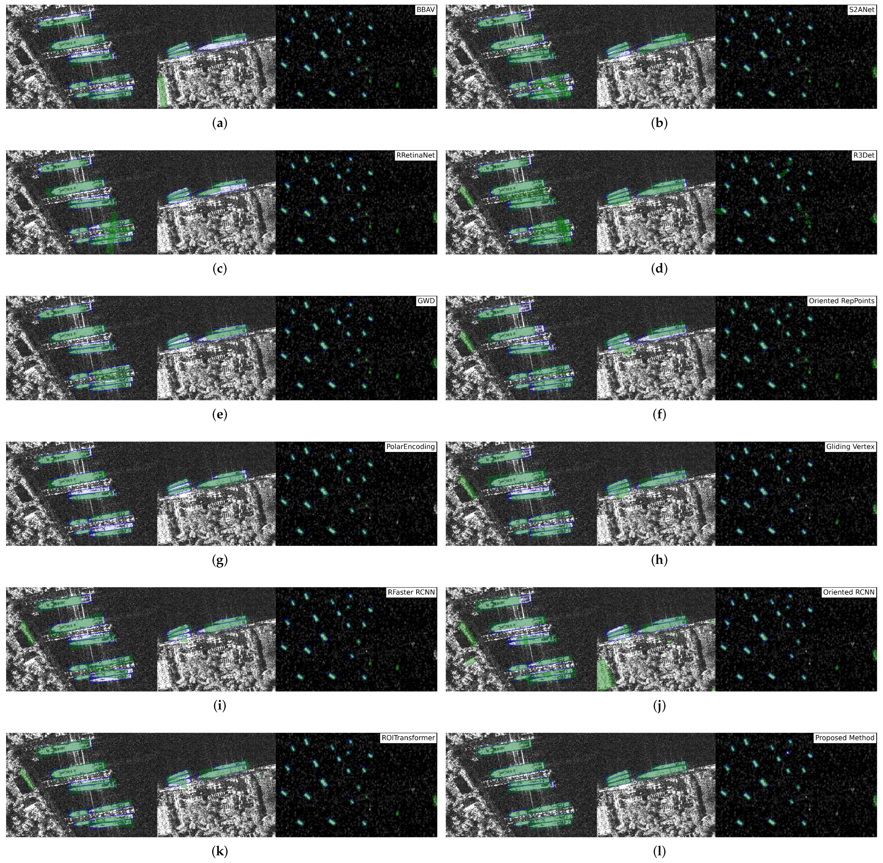
Figure 12 shows the visual results of KeyShip and the compared methods on SSDD. Two inshore images and one offshore image are selected to illustrate the detection results under different scenarios with variant target sizes. To provide a clear indication of the localization accuracy of each method, both the ground truth boxes and the detection results are drawn on the images. Most of the compared methods do not produce satisfactory detection results in the inshore scenarios, failing to generate enough OBBs to cover all the targets, especially the large ones. They also tend to produce many false alarms on the land and large targets, have difficulty detecting crowded targets and incorporate parallel targets into one OBB.

Our proposed method is free of these problems in the inshore scenarios. It correctly identifies each individual ship target and produces OBBs that tightly enclose the ground truth boxes. In the offshore scenario, all the compared methods successfully detect all the targets, but some of them output many false alarms, as in the inshore scenarios. Our method fails to identify the smallest target and generates a false alarm, consistent with the quantitative result that our method fails to achieve the best $A{P}_{m50}$. However, our method produced more high-quality OBBs visually, which further validates the capability of our proposed method to produce accurate detection results.

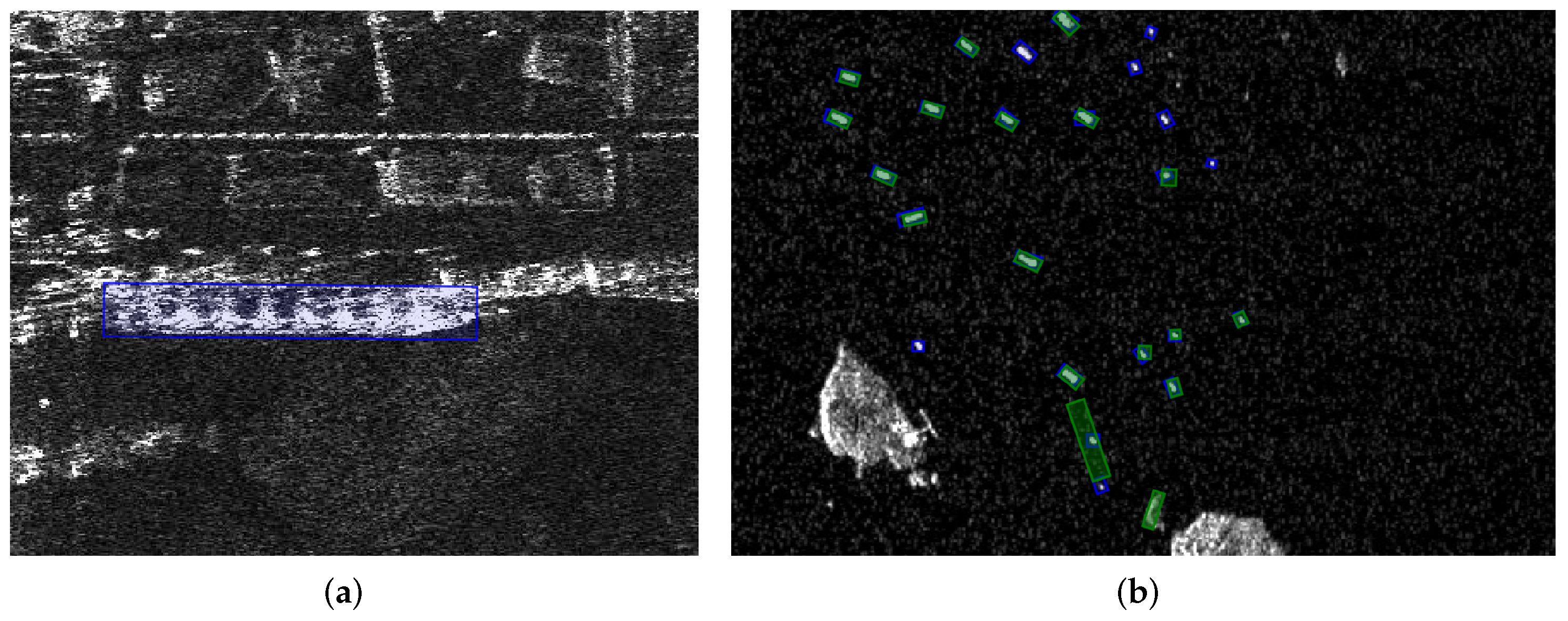
Figure 13 presents some typical false cases of our method. In Figure 13a, the ship target is missed because it is too similar to the harbor and therefore lacks sufficient semantic information about its key parts. In Figure 13b, some small ship targets are also missed, and an unreasonable large OBB is produced. It seems that the shape descriptor at the center of the OBB happens to cluster two SCs from the surrounding targets. More robust feature learning methods and wiser test-time pipelines could be the key to solving these problems, which would be investigated in our future work.

5. Discussion

The results of the ablation study in Section 4.6 provide strong evidence that detecting key points located at the borders of ship targets can produce more precise detection results than simply regressing the ship shapes from the center features, which is a common method used by some one-stage object detectors. This finding supports the theory mentioned in Reference [30] and suggests that the nature of CNNs is to extract local features, making it difficult to obtain information about the target’s boundary and regress the target shape accurately.

In addition, our experiments validate the feasibility of representing ships in SAR imagery as a set of predefined key points, even though these key points may be inconsistent across images and ship targets under SAR imaging and have no strong connections to SAR scattering. The use of plentiful training samples obtained from human annotations allows for the generalization of diversified SAR ships into constant sets of key points.

This article also introduces the shape descriptor and the soft edge point assignment strategy, which are demonstrated to be effective in Section 4.5. The proposed soft edge point assignment strategy is a flexible approach to handling the boundary problem and offers a solution when training a “one-to-many” scenario. For example, when there is a task that requires the neural network to regress an angle a that is periodic, it is better to choose the closest training target to the network output from the set $\left\{a+{360}^{\circ }\times K,K\in Z\right\}$. The results of our experiments suggest that the proposed strategy is an effective solution to this problem.

In summary, the experiments conducted in this paper provide valuable insights into the performance of KeyShip and demonstrate the effectiveness of the proposed methods for ship detection in SAR imagery. The findings in this study have important implications for future research in the field of accurate ship detection and could inspire new approaches for solving the boundary problem in other object detection tasks. However, we acknowledge that our study lacks a detailed investigation of SAR properties such as different wavelengths, which could be a potential weakness. Unfortunately, due to data availability constraints, we were not able to evaluate the proposed technique at different wavelengths. Nonetheless, we believe that this is an important issue to consider in future work, as different wavelength data can significantly impact the scattering properties of targets and may require adapting or modifying our key-point-based approach. However, we are confident that our approach can still be effective at different wavelengths if our model is trained with ample data. Overall, we would like to highlight the potential impact of SAR properties on our proposed technique and emphasize the need for future work to investigate this further.

6. Conclusions

In conclusion, our KeyShip model provides a novel approach to oriented ship detection in SAR images, achieving high-precision detection results through a combination of CNNs with SC and LC branches. Our proposed method uses a shape descriptor to cluster scattered key points and construct OBBs, enabling an accurate representation of ship shapes. Experimental results on SSDD, RSDD, and HRSC2016 datasets demonstrate the high performance and robustness of KeyShip in detecting SAR ships with arbitrary orientations. The success of our proposed approach reaffirms the significance of key point detection in achieving high-precision detection results and highlights the potential of using key points for object detection in remote sensing. Our work presents a new direction in SAR ship detection and demonstrates the potential for using shape descriptors and soft edge point assignment strategies in other OBB-based detection methods. We believe that our proposed approach can be extended to other areas of object detection and make a significant contribution to the field of remote sensing.