Article

Weather Radar Super-Resolution Reconstruction Based on Residual Attention Back-Projection Network

1
College of Electronic Engineering, Chengdu University of Information Technology, Chengdu 610225, China
2
State Key Laboratory of Severe Weather, Chinese Academy of Meteorological Sciences, Beijing 100081, China
3
Key Open Laboratory of Atmospheric Sounding, China Meteorological Administration, Chengdu 610225, China
*
Author to whom correspondence should be addressed.
Remote Sens. 2023, 15(8), 1999; https://doi.org/10.3390/rs15081999
Submission received: 29 December 2022 / Revised: 25 February 2023 / Accepted: 6 April 2023 / Published: 10 April 2023
(This article belongs to the Special Issue Synergetic Remote Sensing of Clouds and Precipitation)

Abstract

:
Convolutional neural networks (CNNs) have been utilized extensively to improve the resolution of weather radar. Most existing CNN-based super-resolution algorithms using PPI (Plan position indicator, which provides a maplike presentation in polar coordinates of range and angle) images plotted by radar data lead to the loss of some valid information by using image processing methods for super-resolution reconstruction. To solve this problem, a weather radar that echoes the super-resolution reconstruction algorithm—based on residual attention back-projection network (RABPN)—is proposed to improve the the radar base data resolution. RABPN consists of multiple Residual Attention Groups (RAGs) connected with long skip connections to form a deep network; each RAG is composed of some residual attention blocks (RABs) connected with short skip connections. The residual attention block mined the mutual relationship between low-resolution radar echoes and high-resolution radar echoes by adding a channel attention mechanism to the deep back-projection network (DBPN). Experimental results demonstrate that RABPN outperforms the algorithms compared in this paper in visual evaluation aspects and quantitative analysis, allowing a more refined radar echo structure, especially in terms of echo details and edge structure features.

Graphical Abstract

1. Introduction

Weather radar not only plays an essential role in meteorology, but it is also used in a variety of fields, such as biology [1,2], urban hydrology [3], geophysical [4], and vocanology [5]. Its all-weather, all-day capability makes it an indispensable tool for detecting precipitation systems and providing early warnings for severe weather events, such as heavy rain, squall lines, hail, and tornadoes. The China New Generation of Weather Radar (CINRAD) uses system echoes to quantify precipitation and monitor extreme weather conditions. The higher the radar resolution, the more detailed the structures of the detected weather targets become, enabling earlier warnings for potential catastrophic weather events.
In weather radar applications, certain regions may not be monitored due to factors, such as the scanning strategy of a radar, the curvature of the earth, and obstructions from terrain. This leads to a lack of comprehensive and objective data for studying various atmospheric patterns. The current CINRAD radar is limited by its spatial and temporal resolution, making it challenging to effectively monitor the rapidly changing severe weather conditions. CINRAD, based on a mechanical scanning system, also faces several challenges in detecting the fine structures of weather processes [6]. These challenges include (1) low spatial resolution with a distance resolution of 1 km, making it difficult to refine the observation weather processes; (2) a volume scan time of 5–6 min, with limited ability to track the evolution of strong weather systems; and (3) a volume coverage pattern of 9 or 14 elevation angles results in limited vertical detail. The medium- and small-scale weather processes, which can span only a few kilometers, are typically represented as a dozen valid range bins in the CINRAD radar echoes, making it challenging to observe the evolution of weather processes.
The Center for Collaborative Adaptive Sensing of the Atmosphere (CASA) in Dallas–Fort Worth (DFW) has established a state-of-the-art urban demonstration network to address weather-related problems. The network consists of eight X-band radar and a National Weather Service S-band radar system [7]. The DFW network observation experiments have shown that radar co-observation technology has better spatial–temporal resolution than a single radar product, and can provide refined observation of the target, which is conducive to the identification of weather systems [8]. In recent years, China has commenced collaborative network observation studies. In 2015, the Foshan Meteorological Bureau built four X-band dual-polarization radars to monitor and warn against strong convection and tornadoes in the Foshan area [9]. The Beijing Meteorological Bureau also deployed five X-band dual-polarization weather radars to overcome blind spots in low-altitude radar detection and enhance weather prediction and warning accuracy [10]. The S-band radar system operates differently from the X-band radar. The S-band radar updates every 5 to 6 min, whereas the X-band radar produces a volume every minute. The X-band radar has a 30∼150 m radial resolution and a detection distance of 60 km. The S-band radar has a 1 km radial resolution and a detection distance of 460 km. The X-band radar has a high resolution but a short detection distance, while the S-band radar has a low resolution but a long detection distance, as shown in Table 1. To address these differences, the S-band radar distance is mapped onto a 250 m × 250 m grid (original distance resolution of 1 km) by using super-resolution algorithms. Therefore, the X-band radar and the S-band radar can be used in combination to effectively make up for their respective shortcomings for refined detection of severe weather events, such as strong convective storms.
The current research on improving radar resolution can be divided into two categories: modifying the radar system hardware and using radar signal processing. The first category involves modifying the radar system hardware. For example, Shinriki et al. [11] used the least-error shaping filters by compressing the outputs to the desired pulse width (the elapsed time between two points with 50 % of the pulse peak value) to reduce the size of the range side-lobes (the lobes (local maxima) of the far field radiation pattern of an antenna or other radiation source) after compression, and the schemes effectively improved the range resolution for the targets. Mar et al. [12] applied the pulse compression technique of the linear frequency modulation (LFM) pulse modulation to improve the range resolution. Zhang et al. [13] verified that Angular Interferometry (AI) can improve the azimuthal resolution of radar and Range Interferometry (RI) can improve the distance resolution of radar using interferometric techniques and demonstrated the feasibility of this method in practical applications. However, the hardware-based approach implies the improving and updating of the radar transmitter, antenna, and receiver, an impractical approach for the new generation of Doppler weather radars currently in operation. The second category uses radar signal processing to analyze radar echoes of redundant information or correlations resulting in the reconstruction of radar data with higher resolution. Wood and Brown et al. [14,15] proposed a super-resolution algorithm of increasing the radial sampling interval to reduce the effective width of the radar antenna beam, and, based on this research result, the U.S. added a 0.5° elevation scan and a data scan mode with a distance resolution of 250 m to the WSR-88D radar in the observation mode. Ruzanski et al. [16] used an improved interpolation method applied to weather radar data to perform windowing and preserved the important echo structure features. Yuan et al. [17] applied different regularization constraints to the sparse representation algorithm to improve the resolution of radar echo data. Zhang et al. [18] proposed the Total Variation-Sparse (TV-Sparse) algorithm, which effectively improves the angular resolution and preserves the contour features of important targets. However, super-resolution algorithms based on these methods may be influenced by the statistical characteristics of radar data and their performance may be impacted by parameters. The deep learning algorithm can effectively overcome these limitations and their performance can be further improved with more observation data samples.
With the advancement of convolutional neural networks (CNNs), super-resolution algorithms have gained significant attention in various fields, including remote sensing [19,20], medical [21,22], agriculture [23,24], and video surveillance [25]. Researchers began to apply super-resolution algorithms based on neural networks to the field of meteorology. Geiss et al. [26] used U-net combined with several densely connected blocks to learn precipitation features, and the reconstructed image results were better than conventional interpolation schemes in terms of objective evaluation metrics and visual quality. Chen et al. [27] applied a generative adversarial network to sub-images of 500 radar images and obtained improved perceptual quality and better peak signal-to-noise ratio (PSNR)/structural similarity index (SSIM) results compared to non-local self-similarity sparse representation. Yuan et al. [28] proposed a non-local residual network that uses radar reflectivity images as a dataset to recover more information about the edge details of the precipitation echo structure.
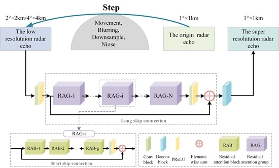
The current approach to enhance radar resolution with CNNs involves super-resolution reconstruction of radar data represented as PPI images. However, the radar data have been quantified when converted into images, resulting in the loss of important information. To address this, the proposed method in this paper aims to reconstruct high-resolution radar echoes directly from radar data, retaining more of the original information and improving the quality of the super-resolution reconstruction. To achieve this, firstly, the paper introduces a residual attention back-projection network (RABPN) which can recover detailed radar echo features and retain more of the original echo information. Additionally, a residual attention block (RAB) is proposed by introducing a channel attention mechanism into the deep attention back-projection network (DBPN). The network structure of [29] network structure uses iterative up- and down-sampling to leverage the interdependence between low- and high-resolution radar echoes compared with the predefined up-sampling [30,31,32] and single up-sampling [33,34] network structures, and the channel attention mechanism [35] can selectively extract relevant information to refine the structure of the radar echoes. To further improve the network’s effectiveness, long and short skip connections [36] are added to the network to prevent the network becoming too deep and avoiding issues with gradient disappearance or gradient explosion.
The rest of the paper is structured as follows. In Section 2, we provide a comprehensive overview of the weather radar super-resolution reconstruction model. In Section 3, we delve into the technical details of the residual attention back-projection network (RABPN). In Section 4, we present a thorough evaluation of the experimental results, including both qualitative and quantitative analyses. Finally, in Section 5, we provide a conclusion and outline potential avenues for future research.

2. Weather Radar Super-Resolution Reconstruction Model

The impact of factors, such as radar beam width (the angular distance between the half power points), the offset produced by the radar elevation angle lifting, and noise, leads to a decrease in radar resolution during weather radar detection. As the detection distance increases, the radar beam tension angle widens and the resolution worsens. Taking CINRAD-SA’s 1° beamwidth as an example, when the weather radar detection distance is 400 km, the azimuth resolution has increased to 6.89 km, which reduces the measurement accuracy of weather targets, as is depicted in Figure 1 and Table 2.
The acquisition of weather radar echo is distinct from that of videos and images captured by cameras, and the degradation model for radar echo is not the same as that used in optical imaging models. The accuracy of the degradation model approximation can determine the proximity of the super-resolution reconstructed echoes to the actual situation. By establishing a low-resolution observation model for radar echo resolution, the degradation process during the acquisition of radar echo is simulated, as is shown in Figure 2.
The degradation model of weather radar, also known as the low-resolution observation model, is generated by simulating the operations of movement, blurring, down-sampling, and noise addition. Movement is a shifting operator; blurring represents a point spread function to simulate the radar echo of blurring; down sampling is achieved through neighborhood averaging of high-resolution echoes; noise is zero-mean Gaussian white noise to simulate system noise introduced during the acquisition, transmission, and storage of weather radar echoes. The degradation process can be equated to the convolution of a point spread function and the radar high-resolution echo, as is shown in Equation (1):
y = A x + n
where x represents the original radar high-resolution echo, y represents the observed low-resolution radar echo, n is the zero-mean Gaussian additive noise, and A is the degenerate matrix, which encompasses the point-based diffusion function and downsampling.
The process of super-resolution reconstruction for weather radar echoes involves solving an underdetermined, inversed problem [37]. The slight modification in input echo data, such as noise, receiver offset, and atmospheric perturbation, might have a significant impact on the reconstructed echoes. Over the years, various regularization methods [38,39,40] have been proposed to solve the ill-posed problem, but these methods require manual modeling, and the accuracy of modeling affects the the quality of reconstruction results. To overcome these challenges, this paper utilizes deep convolutional neural networks (DCNNs) based on a data-driven approach for end-to-end radar data reconstruction. By learning the non-linear mapping relationship between low-resolution (LR) and high-resolution (HR) radar echoes from radar data without manual modeling, the super-resolution reconstruction has excellent generalization performance. The details of the network structure are described in Section 3.

3. Residual Attention Back-Projection Network

3.1. Network Structure

As is depicted in Figure 3, the structure of the network is composed of three parts: shallow feature extraction, deep feature extraction, and reconstruction. Let I l r and I s r be LR and SR (Super resolution) weather radar echo with M l r × N l r and M s r × N s r , respectively, where M l r < M s r and N l r < N s r , M, and N represent radial and distance bins, respectively. As investigated in [41,42], convolutional layer and Parametric Rectified Linear Unit (PReLU) activation [43] are used to extract the shallow feature F 0 from the LR input,
F 0 = H S F I L R
where H S F denotes the convolutional layer with activation PReLU. F 0 is used as the input of RAG deep feature extraction (i.e., depth feature extraction). The i - th RAG feature F R A G i is represented as Equation (3),
F R A G i = H R A G i F 0 , i = 1 , H R A G i F R A G i 1 , i = 2 , , N
where H R A G i denotes the i - th residual attention group with the total number of N. To avoid issues with vanishing or exploding gradients [33], long and short skip connections are employed to effectively facilitate the flow of echo information. The output of the deep feature extraction stages F O U T is represented as Equation (4).
F O U T = H C O V F R A G N + F 0
where H C O V denotes the convolution modules and the PReLU activation function. To reconstruct the high-resolution radar echoes, the deconvolution layer [44] was selected.
I S R = H R A B P N I L R = H R E C F O U T
where H R E C and H R A B P N denote the reconstruction layer and the function of proposed residual attention back-projection network, respectively.

3.2. Residual Attention Groups (RAG)

We were inspired by the work of Zhang et al. [45] and Liu et al. [46], who, respectively, constructed a Residual in Residual (RIR) structure for learning residual information and constructed Enhanced Residual Blocks (ERB) that enabled a network to benefit from residual structures. Therefore, we added skip connections simultaneously in the network for better learning of feature information.
To enhance the focus of the main network on crucial features, a short skip connection is introduced in the RAG internal module, as demonstrated in Equation (6),
F R A G i = F R A G i 1 + H C O V F R A B g , i = 2 , , N
where F R A B g represents the g - th RAB feature and is defined as the following equation,
F R A B g = H R A B g F R A B g 1 = H R A B g H R A B g 1 H R A B 2 H R A B 1 F R A G i 1
where H R A B g 1 denotes the g - 1 - th residual attention block with the total number of g. As is shown in Figure 4, to explicitly model the interdependencies between convolutional feature channels, a channel attention mechanism (CAM) is added to up-projection and down-projection units constituting RAB, where up-projections and down-projections mutually learn the layers of critical information and CAM denotes the channel attention mechanism that can selectively emphasize the information characteristics of strong radar echo areas. The C represents the concatenate function. The outputs of the down-projection units are directly concatenated, except for the last projection unit, where CAM is added as an output.

3.2.1. The Up- and Down-Projection Unit

As is illustrated in Figure 5, up- and down-projection units consist of three operations, convolution, deconvolution, and PReLU activation. These units work iteratively, alternating the solution by feeding back-projection errors between LR and HR components, resulting in improved performance on the large scaling factor.
For the up-projection unit, the radar echo H t consists of the sum of the radar echoes generated by the first upsampling layer H 0 t and the radar echoes generated by the second up sampling layer H 1 t , as is shown in Equation (8):
H t = H 0 t + H 1 t
The first up sampling layer output:
H 0 t = F c , ac L t 1 s
The down sampling layer output:
L 0 t = F dc , ac H 0 t s
The second up sampling layer output:
H 1 t = F c , ac e l t s = F c , ac L 0 t L t 1 s
where F c , a c denotes the convolution and activation operators, F d c , a c denotes the deconvolution and activation operators, s represents the upsampling operator with scale factor s, s represents the downsampling operator with scaling factor s. The residual between the input LR radar echo L 0 t and the echo L t 1 generated by the down-sampling layer is e l t . The structure of the down-projection unit is similar to that of the up-projection unit, except that the down-projection unit maps HR radar echo H t to LR radar echo L t .

3.2.2. The Channel Attention Mechanism (CAM)

The attention mechanism facilitates integration into existing networks to improve network performance at a low cost. By modeling the importance between radar echo features, distinguished feature assignments are made for the low- and high-frequency components of the LR radar echoes, and the reconstructed HR radar echo can achieve more refined structure. As is shown in Figure 6, GP represents the operation of global average pooling, the reduction ratio r introduced is a hyperparameter which allows us to vary the capacity and computational cost of the CAM blocks in the network.
Let I = i 1 , i 2 , , i c is the input of the channel attention mechanism, with a total of C feature maps of size H × W . The channel statistic Z R 1 × 1 × C is obtained by compressing the input through spatial dimensions H × W , the c - th element of z c is shown in Equation (12).
z c = F G P i c = 1 H × W i = 1 H j = 1 W i c ( i , j )
where i c ( i , j ) represents the value at position ( i , j ) of c - th feature i c , unlike the image, H and W represent radial and distance bins, respectively. F G P denotes the global pooling function. To fuse the feature map information of each channel, a structure containing two fully connected layers (FCs) is adopted, the first FC layer plays a role in reducing dimensionality, and the second FC layer restores the original dimension. As described in [35], adding the ReLU (Rectified Linear Unit) function [47] after the first FC layer and sigmoid activation function after the second FC layer allows for better adaptation to the complex correlations between channels, learning non-mutually exclusive relationships between channels. The final channel statistic S is obtained, as shown in Equation (13).
S = f ω S h ω R Z
where ω S and ω R are the weight parameters to be trained, f ( · ) and h ( · ) represent sigmoid activation functions and ReLU functions, respectively. The output of the channel attention mechanism I = i 1 , i 2 , , i c is obtained by rescaled from the channel statistic S to the input I, taking the c - th feature map as an example, as is shown in Equation (14):
i c = S c · i c
where s c and i c R H × W represent the scaling factor and feature map in the c - th channel.

4. Experimental Results

4.1. Parameter Settings

In the degradation model of weather radar, as shown in Figure 2, the noise standard deviation sigma ( σ ) is set as 1.5 [48]; the scaling factor adopts ×2 and ×4 factor in the training stage, the number of training sample is 10,000, and the batch size is set as 20 in each epoch round with a total of 500 iterations. The learning rate is initialized as 10 4 and decreased by a factor of 10 for every 1000 iterations. Adam optimizer [49] is used to this paper with momentum to β 1 = 0.9 , β 2 = 0.99 and e p s = 10 8 . The loss function is chosen as L1 loss [44,45,50], and is defined as follows:
L ( Θ ) = 1 N i = 1 N H R A B P N I i l r I i h r 1
where I i h r represents high-resolution radar echoes and H R A B P N I i l r represents reconstructed radar echoes in a batch of N, and Θ denotes the parameters to be trained. Each network model was built on PyTorch [51] (version 1.4.0) and Python (version 3.8), and the training model (RABPN) used a Tesla P40 GPU for about 8 days.

4.2. Datasets

In this paper, the reflectivity data products from the CINRAD-SA radar are used. To increase the diversity of the dataset and to verify the effectiveness of RABPN in detecting medium- and small-scale extreme weather processes, a 32 × 32 sliding window [52] is adopted to synthesize training data. This includes the rainfall data in South China Heavy Rainfall Observation taken in August 2011, May and June of 2015, and the tornado data taken in July 2011, August 2013, July 2015, and August of 2017. The first elevation cut (0.5° elevation) is adopted in this paper to observe echo intensity. As is shown in Figure 7, the 32 × 32 (radials × range bins) window, with a step size of 2, is moved to the right until it reaches the rightmost position, then moved down two steps and the process is repeated until the window reaches the last position. Inevitably, the 32 × 32 (radials × distance bin) blocks contain some invalid information, and the data preprocessing operation of discarding invalid blocks are performed.

4.3. The Number of RAG and RAB

To determine the optimal number of RAG and RAB in our network, five groups of experiments were compared, namely 1 residual group and 2 residual blocks (RABPN-G1), 2 residual groups and 4 residual blocks (RABPN-G2), 3 residual groups and 6 residual blocks (RABPN-G3), 4 residual groups and 8 residual blocks (RABPN-G4), and 5 residual groups and 10 residual blocks (RABPN-G5). To intuitively compare the five groups of experiments, we draw four broken line graphs on different sampling scaling factors in different weather systems, where the dotted line represents the PSNR values of DBPN under the specific experimental conditions, as is shown in Figure 8. The graph in Figure 8a displays five groups PSNR values in the medium weather system on the scale factor ×2, Figure 8b displays five groups PSNR values in the small weather system on the scale factor ×2, Figure 8c displays five groups PSNR values in the medium weather system on the scale factor × 4, and Figure 8d displays five groups PSNR values in the small weather system on the scale factor × 4.
In [50,53] it was found that increasing the depth of a model may lead to decreased shallow learning ability and gradient instability. Despite attempts to mitigate network degradation, performance decreases as the number of groups increases. Thus, we conduct five experiments to determine the optimal network depth.
Table 3 shows that for the scale factor ×2, the medium weather system achieved a maximum PSNR value of 36.93 dB and the small weather system achieved a maximum PSNR value of 40.66 dB using the RABPN-G2 network. For the scale factor ×4, the medium weather system achieved a maximum PSNR value of 33.04 dB and the small weather system achieved a maximum PSNR value of 34.70 dB using the RABPN-G4 network. Considering the superiority of the results across different weather systems, the RABPN network structure with 4 residual groups and 8 residual blocks groups was selected.

5. Results

To evaluate the accuracy of the reconstruction results of the RABPN model and validate its performance, two representative examples were selected for testing and were analyzed through visual and quantitative evaluations. Considering that catastrophic weather can be of great help to us in monitoring and providing early warning about medium- and small-scale extreme weather if early warnings can be carried out, this paper reconstructs the one-hour echo data, and the specific visualization results are shown in the Appendix A and Appendix B. To validate the performance of RABPN network, the visual results and the quantitative results by peak signal-to-noise ratio (PSNR)/structural similarity index (SSIM) were analyzed. LR radar echoes are generated by down-sampling HR radar echoes with specific scaling factors, PSF functions, and noise addition. The LR echoes were used as an input for the super-resolution reconstruction and the high-resolution echoes were obtained through the interpolation reconstruction learning method.
The selected case of the medium-scale weather system took place at 9:30 on 15 May 2016 in Heyuan, Guangdong, China and was characterized by intense precipitation with strong precipitation activity indicated in red (≥40 dBZ) in Figure 9. On the other hand, the selected case of the small-scale weather system took place at 14:08 on 23 June 2016 in Yancheng, Jiangsu, China and involved a tornado event. This event is shown in the black box of Figure 9, which displays a tornado vortex feature located at the end of the hook echo. The PPI map displays a strong reflectivity feature with an intensity of about 55 dBZ.
Visual Comparison. Visual comparisons on the scale factor ×2 and the scale factor ×4 is shown in Figure 10 and Figure 11. The scale factor ×2 represents a two-times increase in range and radial resolution of reflectivity, and the LR echoes’ resolution increased from algorithms increased from 2 km × 2 to 1 km × 1 ; the scale factor ×4 represents 4 times increase in range and radial resolution of reflectivity, and the LR echoes’ resolution increased from 4 km × 4 to 1 km × 1 ). As is shown in Figure 10, the RABPN model outperforms interpolation-based methods in terms of recovering more detailed echo features in the precipitation process. The interpolation-based method tends to lose some important information in the strong echoes, leading to too smooth radar echoes. In comparison to other deep learning-based models, such as SRCNN (Super Resolution Convolutional Network) [30], FSRCNN (Fast Super-Resolution Convolutional Neural Network) [33], ESPCN (Efficient Sub-pixel Convolutional Neural Network) [34], EDSR (Enhanced Deep Super-resolution Network) [41], VDSR (Very Deep Convolutional Network) [31], and DBPN (Deep Back-Projection Network) [29], RABPN effectively captures the interrelationship between the low-resolution radar echoes and the original echoes, resulting in better recovery of detailed radar echo features and retention of more information from the original echoes. Although there may still be differences between the reconstructed echoes using RABPN and the original echoes, RABPN effectively recovers the texture features of the strong echo regions and highlights the locations of the strong echoes. This makes RABPN a valuable tool for researching and forecasting heavy precipitation weather.
Tornadoes are small-scale convective vortexes produced under unstable weather conditions, with short lifespans and high catastrophic potential. Most tornadoes, especially those above EF-2, occur mainly in supercell storms, and the hook echo is the region where tornadoes can occur in supercell thunderstorms [54]. The tornado vortex feature can serve as an early warning signal, characterized by a strong reflectivity feature on the PPI map (approximately 55 dBZ), as shown in the black box in Figure 11, which exhibits a strong reflectivity feature on the PPI map with an intensity of about 55 dBZ. However, the limited resolution of the CINRAD-SA radar often hinders the effective observation of the tornado formation and termination process. By reconstructing the hook echo and vortex features as accurately as possible, we can improve the monitoring and providing early warnings for tornado weather conditions.
For a scale factor ×2, the neural network-based method can recover a portion of the hook echoes and can restore information on the edge details of the echo structure compared to the interpolation-based method. For scale factor ×4, most comparison methods produce blurred results; however, RABPN can recover more echo details and hook features. Despite being unable to recover the detailed structure of the hook echo compared to the original radar echo at both scale factors, RABPN is still able to accurately recover the hook echo and highlight the location of strong echoes. This makes it great helpful for our monitoring and providing early warning of small-scale extreme disaster weather, such as tornadoes.
Quantitative results by PSNR/SSIM. PSNR and SSIM [55] were selected to verify the reconstruction quality of radar echo and the similarity with the original echo resolution, respectively. The radar echo size is H × W , f ( i , j ) denotes the original high-resolution echo, and f ^ ( i , j ) denotes the reconstructed echo, then the PSNR has the following definition:
M S E = 1 H × W i = 1 H j = 1 W ( f ( i , j ) f ^ ( i , j ) ) 2
P S N R = 10 log 10 255 2 M S E
PSNR measures the reconstruction quality by quantifying the difference between the original and reconstructed radar echoes, with higher values indicating better performance. Considering the correlation between adjacent distance library values and the perceptual properties of the human visual system, the paper uses the SSIM metric to evaluate the structural characteristics of the echoes, as is shown in Equation (18).
SSIM = 2 u x u y + c 1 2 σ x y + c 1 u x 2 + u y 2 + c 1 σ x 2 + σ y 2 + c 2
where u x and u y denote the mean values of the original high-resolution echo and the reconstructed echo, respectively. σ x and σ y denote the standard deviation of the original high-resolution and reconstructed echoes, respectively. σ x y denotes the covariance between the two. c 1 and c 2 denote two constants to avoid the denominator being zero and maintain the stability of the results. SSIM values range from 0 to 1, where a higher value indicates closer similarity between the original and reconstructed radar echoes in terms of structure. The results of the comparison for scale factors ×2 and ×4 is presented in Table 4.
To further validate the effectiveness of RABPN, we compared the proposed RABPN with various SR methods under different weather conditions, such as medium- and small-scale weather systems, and the results showed that RABPN achieved the highest PSNR and SSIM values, indicating that RABPN has better performance. When considering the scale factor ×2, the PSNR values of RABPN are up to 0.14 dB and 0.31 dB higher than DBPN on precipitation and tornado data, respectively; for the scale factor ×4, the PSNR values of RABPN are up to 0.68 dB and 0.72 dB higher than DBPN on precipitation and tornado data, respectively. The comparisons indicates that CAM and the network depth improve the performance. Moreover, since tornadoes have obvious echo characteristics, our network achieves better results in the tornado case than in the precipitation case by utilizing CAM to emphasize the information characteristics of the strong radar echo region. This result demonstrate that networks with more representational ability can extract more sophisticated features from the LR radar echoes. When the scaling factor is large, LR radar echoes contain minimal information for SR radar echoes. Losing most high-frequency information makes reconstructing informative results difficult for SR methods.

6. Conclusions

The purpose of this paper was to enhance the spatial resolution of weather radar data. To achieve this goal, CINRAD-SA reflectivity data were used as the training set for a network model, and using RABPN for super-resolution reconstruction of individual cases of small- and medium-scale weather. Through constant parameter tuning, network structure optimization, and continuous debugging, the following main conclusions were drawn:
(1) For precipitation cases, RABPN can recover fine echo edges and details in the scaling factor ×2 and the scale factor ×4, achieving fine reconstruction of the structure of weak and strong echo regions. The results of the quantitative analysis showed that RABPN outperformed other compared super-resolution reconstruction methods in terms of PSNR and SSIM values, demonstrating that the algorithm had superior reconstruction performance and a closer similarity to the original echo structure. This is of great significance for monitoring and providing early warning about catastrophic weather processes.
(2) For the tornado case, RABPN can effectively recover the hook echo characteristics of the tornado, enabling the reconstructed hook echoes to be closer to the real radar echoes. Additionally, RABPN can reasonably recover the strong echo information with echo intensity values above 55 dBZ. Compared with other networks, RABPN has better performance in highlighting strong echoes.
RABPN is composed of multiple residual attention groups (RAG) and residual attention blocks (RAB), which utilize long and short skip connections, respectively, to enable the network to reach a significant depth. Furthermore, by adding the channel attention mechanism to the network means that the concerns between the different channels change for the low- and high-frequency information. Unlike previous CNN algorithms for weather radar that rely on radar image reconstruction, this paper adopts raw radar data in order to preserve crucial information in the weather radar echoes.
Extensive results illustrated that our proposed network provides a more nuanced view of the internal structure of the echoes and clearer edge details compared with the previous CNN radar image reconstruction, particularly in the scaling factor. It is worth noting that the vertical structure of radar is essential for the in-depth study of the generation and elimination process of disastrous weather. Currently, the majority of focus in this research area is on reconstructing the horizontal structure, and the application of vertical structure in the weathering process leaves much to be desired. In the future, deep learning algorithms have the potential to enhance the resolution of vertical structure data, enable multi-radar super-resolution data fusion, and generate high spatial and temporal resolution vertical structure data.

Author Contributions

Conceptualization, Q.Y., M.Z., Q.Z. and H.W.; methodology, Q.Y., M.Z. and Q.Z.; software, Q.Y., M.Z. and Q.Z.; validation, Q.Y., Q.Z. and Q.C.; formal analysis, Q.Y., Q.Z. and X.F.; investigation, Q.Z.; resources, Q.Z. and H.W.; data curation, Q.Z.; writing—original draft preparation, Q.Y.; writing—review and editing, Q.Y., M.Z. and Q.Z.; visualization, Z.Q. and Q.C.; supervision, Q.Z., H.W. and Q.C.; project administration, Q.Z. and Z.Q.; funding acquisition, Q.Z. All authors have read and agreed to the published version of the manuscript.

Funding

This research was funded by the National Natural Science Foundation of China (U20B2061), the Open Grants of the State Key Laboratory of Severe Weather (2020LASW-B11), Sichuan Department of Science and Technology (2023NSFSC0244, 2022YFS0541), the Joint Research Project for Meteorological Capacity Improvement (22NLTSY009), the fund of Key Laboratory of Atmosphere Sounding (2021KLAS01M, 2022KLAS01Z), Key Scientific Research Projects of Jiangsu Provincial Meteorological Bureau (KZ202203) and the Key R&D Program of Yunnan Provincial Department of Science and Technology (202203AC100021), Key Grant Project of Science and Technology Innovation Capacity Improvement Program of CUIT (KYQN202217).

Data Availability Statement

The authors used CINRAD SA radar tornado information from Jiangsu Province and precipitation information from South China, Guangdong Province, and it was greatly appreciated. The authors also thank the published researchers whose literature contains the information used and cited in this paper.

Conflicts of Interest

The authors declare no conflict of interest.

Abbreviations

The following abbreviations are used in this manuscript:
AIAngular Interferometry
CASAThe collaborative adaptive sensing of the atmosphere
CAMThe channel attention mechanism
CNNsConvolutional neural networks
CINRADThe China new generation of weather radar
CAMChannel attention mechanism
DBPNDeep Back-Projection Network
DFWDallas-Fort Worth
EDSREnhanced Deep Super-resolution Network
ERBEnhanced Residual Blocks
ESPCNEfficient Sub-pixel Convolutional Neural Network
FCFully connected layers
FSRCNNFast Super-Resolution Convolutional Neural Network
HRHigh-Resolution
LFMthe linear frequency modulation
LRLow-Resolution
PPIThe plan position indicator
PReLUParametric Rectified Linear Unit
PSNRPeak signal-to noise ratio
ReLURectified Linear Unit
RABPNResidual attention back-projection network
RABResidual Attention Blocks
RAGResidual Attention Groups
RIRResidual in Residual
RIRange Interferometry
SRSuper Resolution
SRCNNSuper Resolution Convolutional Network
SSIMStructural similarity index
TV-SparseTotal Variation-Sparse
VDSRVery Deep Convolutional Network

Appendix A

The detailed network configurations of SRCNN, FSRCNN, ESPCN, EDSR, VDSR, DBPN, and RABPN are described in Table A1 and Table A2.
Table A1. ‘Conv’ and ‘DeConv’ refer to the convolutional layer and deconvolutional layer, respectively. ‘Sub-pixel Conv’ refers to the sub-pixel convolutional layer. ‘BP stages’ represents a sequence of projection units including up- and down-projection units.
NameInput SizeTypeLayerKernel SizeNumber
SRCNN S HR ConvConv19 × 91
Conv25 × 51
Conv35 × 51
FSRCNN S LR Conv, DeConvConv15 × 51
Conv21 × 11
Conv33 × 34
Conv41 × 11
DeConv9 × 91
ESPCN S LR Conv, Sub-pixel ConvConv15 × 51
Conv23 × 31
Sub-pixel3 × 31
EDSR S LR Conv, Residual block(s)Conv13 × 31
Residual blocks3 × 316
VDSR S HR Conv, Residual block(s)Conv13 × 31
Residual block3 × 31
DBPN S LR Conv, BP stagesConv13 × 31
Conv21 × 11
BP stages-7
Conv31 × 11
RABPN S LR Conv, RAB, Residual block(s)Conv11 × 11
RAB-32
Residual block(s)3 × 333
DeConv3 × 31
Table A2. The part structure of networks. Note: The use of large-sized filters is avoided because it can slow down the convergence speed and might produce sub-optimal results. However, the iterative up- and down-sampling units enable the mutual relation between LR and HR radar echoes [29].
NameScaleKernel Size
BP stages×26 × 6
×48 × 8
RAB×26 × 6
×48 × 8

Appendix B

Appendix B.1

This appendix shows the reconstructed effect of about one hour of precipitation data with different scaling factors, where a represents the original high-resolution echo, b represents the low-resolution echo, and c represents the reconstructed echo of RABPN. Among them, 1–10 represent the precipitation time occurred at 9:00, 9:06, 9:12, 9:18, 9:24, 9:30, 9:36, 9:42, 9:49, and 9:54 on May 15, 2016, in Heyuan, Guangdong, China, respectively.
Figure A1. Precipitation data on the scaling factor ×2.
Remotesensing 15 01999 g0a1
Figure A2. Precipitation data on the scaling factor ×4.
Remotesensing 15 01999 g0a2

Appendix B.2

This appendix shows the reconstructed effect of about one hour of precipitation data with different scaling factors, where a represents the original high-resolution echo, b represents the low-resolution echo, and c represents the reconstructed echo of RABPN. Among them, 1–10 represent the tornado time occurred at 9:00, 9:06, 9:12, 9:18, 9:24, 9:30, 9:36, 9:42, 9:49, and 9:54 on June 23, 2016, in Yancheng, Jiangsu, China, respectively.
Figure A3. Tornado data on the scaling factor ×2.
Remotesensing 15 01999 g0a3
Figure A4. Tornado data on the scaling factor ×4.
Remotesensing 15 01999 g0a4

References

  1. Dokter, A.M.; Desmet, P.; Spaaks, J.H.; van Hoey, S.; Veen, L.; Verlinden, L.; Nilsson, C.; Haase, G.; Leijnse, H.; Farnsworth, A.; et al. bioRad: Biological analysis and visualization of weather radar data. Ecography 2019, 42, 852–860. [Google Scholar] [CrossRef] [Green Version]
  2. Cui, K.; Hu, C.; Wang, R.; Sui, Y.; Mao, H.; Li, H. Deep-learning-based extraction of the animal migration patterns from weather radar images. Sci. China Inf. Sci. 2020, 63, 1–10. [Google Scholar] [CrossRef] [Green Version]
  3. Thorndahl, S.; Einfalt, T.; Willems, P.; Nielsen, J.E.; ten Veldhuis, M.C.; Arnbjerg-Nielsen, K.; Rasmussen, M.R.; Molnar, P. Weather radar rainfall data in urban hydrology. Hydrol. Earth Syst. Sci. 2017, 21, 1359–1380. [Google Scholar] [CrossRef] [Green Version]
  4. McCarthy, N.; Guyot, A.; Dowdy, A.; McGowan, H. Wildfire and weather radar: A review. J. Geophys. Res. Atmos. 2019, 124, 266–286. [Google Scholar] [CrossRef] [Green Version]
  5. Schneider, D.J.; Hoblitt, R.P. Doppler weather radar observations of the 2009 eruption of Redoubt Volcano, Alaska. J. Volcanol. Geotherm. Res. 2013, 259, 133–144. [Google Scholar] [CrossRef]
  6. Drake, P.R.; Bourgeois, J.; Hopf, A.P.; Lok, F.; McLaughlin, D. Dual-polarization X-band phased array weather radar: Technology update. In Proceedings of the 2014 International Radar Conference, Piscataway, NJ, USA, 13–17 October 2014; pp. 1–6. [Google Scholar]
  7. Chandrasekar, V.; Chen, H.; Philips, B. Principles of high-resolution radar network for hazard mitigation and disaster management in an urban environment. J. Meteorol. Soc. Jpn. Ser. II 2018, 96, 119–139. [Google Scholar] [CrossRef] [Green Version]
  8. Junyent, F.; Chandrasekar, V. Theory and characterization of weather radar networks. J. Atmos. Ocean. Technol. 2009, 26, 474–491. [Google Scholar] [CrossRef]
  9. Li, Z.; Chen, H.; Chu, H.; Tan, H.; Chandrasekar, V.; Huang, X.; Wang, S. Multivariate Analysis and Warning of a Tornado Embedded in Tropical Cyclone in Southern China. IEEE J. Sel. Top. Appl. Earth Obs. Remote Sens. 2021, 14, 11517–11529. [Google Scholar] [CrossRef]
  10. Wang, C.; Wu, C.; Liu, L.; Liu, X.; Chen, C. Integrated correction algorithm for X band dual-polarization radar reflectivity based on CINRAD/SA radar. Atmosphere 2020, 11, 119. [Google Scholar] [CrossRef] [Green Version]
  11. Shinriki, M.; Takase, H.; Sato, R.; Susaki, H. Multi-range-resolution radar using sideband spectrum energy. IEE Proc.-Radar Sonar Navig. 2006, 153, 396–402. [Google Scholar] [CrossRef]
  12. Mar, T.T.; Mon, S.S.Y. Pulse compression method for radar signal processing. Int. J. Sci. Eng. Appl. 2014, 3, 31–35. [Google Scholar] [CrossRef]
  13. Zhang, G.; Yu, T.Y.; Doviak, R.J. Angular and range interferometry to refine weather radar resolution. Radio Sci. 2005, 40, 1–10. [Google Scholar] [CrossRef]
  14. Wood, V.T.; Brown, R.A.; Sirmans, D. Technique for improving detection of WSR-88D mesocyclone signatures by increasing angular sampling. Weather Forecast. 2001, 16, 177–184. [Google Scholar] [CrossRef]
  15. Brown, R.A.; Wood, V.T.; Sirmans, D. Improved tornado detection using simulated and actual WSR-88D data with enhanced resolution. J. Atmos. Ocean. Technol. 2002, 19, 1759–1771. [Google Scholar] [CrossRef]
  16. Ruzanski, E.; Chandrasekar, V. Weather radar data interpolation using a kernel-based lagrangian nowcasting technique. IEEE Trans. Geosci. Remote Sens. 2014, 53, 3073–3083. [Google Scholar] [CrossRef]
  17. Yuan, H.; Zeng, Q.; He, J. Adaptive regularized sparse representation for weather radar echo super-resolution reconstruction. In Proceedings of the 2021 International Conference on Electronic Information Engineering and Computer Science (EIECS), Changchun, China, 23–26 September 2021; pp. 33–38. [Google Scholar]
  18. Zhang, Q.; Zhang, Y.; Huang, Y.; Zhang, Y.; Pei, J.; Yi, Q.; Li, W.; Yang, J. TV-sparse super-resolution method for radar forward-looking imaging. IEEE Trans. Geosci. Remote Sens. 2020, 58, 6534–6549. [Google Scholar] [CrossRef]
  19. Zhang, S.; Wu, R.; Xu, K.; Wang, J.; Sun, W. R-CNN-based ship detection from high resolution remote sensing imagery. Remote Sens. 2019, 11, 631. [Google Scholar] [CrossRef] [Green Version]
  20. Arun, P.V.; Buddhiraju, K.M.; Porwal, A.; Chanussot, J. CNN based spectral super-resolution of remote sensing images. Signal Process. 2020, 169, 107394. [Google Scholar] [CrossRef]
  21. Park, J.; Hwang, D.; Kim, K.Y.; Kang, S.K.; Kim, Y.K.; Lee, J.S. Computed tomography super-resolution using deep convolutional neural network. Phys. Med. Biol. 2018, 63, 145011. [Google Scholar] [CrossRef]
  22. Georgescu, M.I.; Ionescu, R.T.; Verga, N. Convolutional neural networks with intermediate loss for 3D super-resolution of CT and MRI scans. IEEE Access 2020, 8, 49112–49124. [Google Scholar] [CrossRef]
  23. Yamamoto, K.; Togami, T.; Yamaguchi, N. Super-resolution of plant disease images for the acceleration of image-based phenotyping and vigor diagnosis in agriculture. Sensors 2017, 17, 2557. [Google Scholar] [CrossRef] [PubMed] [Green Version]
  24. Yue, Y.; Cheng, X.; Zhang, D.; Wu, Y.; Zhao, Y.; Chen, Y.; Fan, G.; Zhang, Y. Deep recursive super resolution network with Laplacian Pyramid for better agricultural pest surveillance and detection. Comput. Electron. Agric. 2018, 150, 26–32. [Google Scholar] [CrossRef]
  25. Seibel, H.; Goldenstein, S.; Rocha, A. Eyes on the target: Super-resolution and license-plate recognition in low-quality surveillance videos. IEEE Access 2017, 5, 20020–20035. [Google Scholar] [CrossRef]
  26. Geiss, A.; Hardin, J.C. Radar super resolution using a deep convolutional neural network. J. Atmos. Ocean. Technol. 2020, 37, 2197–2207. [Google Scholar] [CrossRef]
  27. Chen, H.; Zhang, X.; Liu, Y.; Zeng, Q. Generative adversarial networks capabilities for super-resolution reconstruction of weather radar echo images. Atmosphere 2019, 10, 555. [Google Scholar] [CrossRef] [Green Version]
  28. Yuan, H.; Zeng, Q.; He, J. Weather Radar Image Superresolution Using a Nonlocal Residual Network. J. Math. 2021, 2021, 4483907. [Google Scholar] [CrossRef]
  29. Haris, M.; Shakhnarovich, G.; Ukita, N. Deep back-projection networks for super-resolution. In Proceedings of the IEEE Conference on Computer Vision and Pattern Recognition, Salt Lake City, UT, USA, 18–23 June 2018; pp. 1664–1673. [Google Scholar]
  30. Dong, C.; Loy, C.C.; He, K.; Tang, X. Image super-resolution using deep convolutional networks. IEEE Trans. Pattern Anal. Mach. Intell. 2015, 38, 295–307. [Google Scholar] [CrossRef] [Green Version]
  31. Kim, J.; Lee, J.K.; Lee, K.M. Accurate image super-resolution using very deep convolutional networks. In Proceedings of the IEEE Conference on Computer Vision and Pattern Recognition, Las Vegas, NV, USA, 27–30 June 2016; pp. 1646–1654. [Google Scholar]
  32. Kim, J.; Lee, J.K.; Lee, K.M. Deeply-recursive convolutional network for image super-resolution. In Proceedings of the IEEE Conference on Computer Vision and Pattern Recognition, Las Vegas, NV, USA, 27–30 June 2016; pp. 1637–1645. [Google Scholar]
  33. Dong, C.; Loy, C.C.; Tang, X. Accelerating the super-resolution convolutional neural network. In Proceedings of the European Conference on Computer Vision, Amsterdam, The Netherlands, 11–14 October 2016; Springer: Berlin/Heidelberg, Germany, 2016; pp. 391–407. [Google Scholar]
  34. Shi, W.; Caballero, J.; Huszár, F.; Totz, J.; Aitken, A.P.; Bishop, R.; Rueckert, D.; Wang, Z. Real-time single image and video super-resolution using an efficient sub-pixel convolutional neural network. In Proceedings of the IEEE Conference on Computer Vision and Pattern Recognition, Las Vegas, NV, USA, 27–30 June 2016; pp. 1874–1883. [Google Scholar]
  35. Hu, J.; Shen, L.; Sun, G. Squeeze-and-excitation networks. In Proceedings of the IEEE Conference on Computer Vision and Pattern Recognition, Salt Lake City, UT, USA, 18–23 June 2018; pp. 7132–7141. [Google Scholar]
  36. Drozdzal, M.; Vorontsov, E.; Chartrand, G.; Kadoury, S.; Pal, C. The importance of skip connections in biomedical image segmentation. In Deep Learning and Data Labeling for Medical Applications; Springer: Berlin/Heidelberg, Germany, 2016; pp. 179–187. [Google Scholar]
  37. Albu, A.I.; Czibula, G.; Mihai, A.; Czibula, I.G.; Burcea, S.; Mezghani, A. NeXtNow: A Convolutional Deep Learning Model for the Prediction of Weather Radar Data for Nowcasting Purposes. Remote Sens. 2022, 14, 3890. [Google Scholar] [CrossRef]
  38. Oliveira, J.P.; Bioucas-Dias, J.M.; Figueiredo, M.A. Adaptive total variation image deblurring: A majorization–minimization approach. Signal Process. 2009, 89, 1683–1693. [Google Scholar] [CrossRef]
  39. Daubechies, I.; Defrise, M.; De Mol, C. An iterative thresholding algorithm for linear inverse problems with a sparsity constraint. Commun. Pure Appl. Math. A J. Issued Courant Inst. Math. Sci. 2004, 57, 1413–1457. [Google Scholar] [CrossRef] [Green Version]
  40. Shi, F.; Cheng, J.; Wang, L.; Yap, P.T.; Shen, D. LRTV: MR image super-resolution with low-rank and total variation regularizations. IEEE Trans. Med Imaging 2015, 34, 2459–2466. [Google Scholar] [CrossRef] [Green Version]
  41. Lim, B.; Son, S.; Kim, H.; Nah, S.; Mu Lee, K. Enhanced deep residual networks for single image super-resolution. In Proceedings of the IEEE Conference on Computer Vision and Pattern Recognition Workshops, Honolulu, HI, USA, 21–26 July 2017; pp. 136–144. [Google Scholar]
  42. Ledig, C.; Theis, L.; Huszár, F.; Caballero, J.; Cunningham, A.; Acosta, A.; Aitken, A.; Tejani, A.; Totz, J.; Wang, Z.; et al. Photo-realistic single image super-resolution using a generative adversarial network. In Proceedings of the IEEE Conference on Computer Vision and Pattern Recognition Workshops, Honolulu, HI, USA, 21–26 July 2017; pp. 4681–4690. [Google Scholar]
  43. He, K.; Zhang, X.; Ren, S.; Sun, J. Delving deep into rectifiers: Surpassing human-level performance on imagenet classification. In Proceedings of the IEEE International Conference on Computer Vision, Santiago, Chile, 7–13 December 2015; pp. 1026–1034. [Google Scholar]
  44. Lai, W.S.; Huang, J.B.; Ahuja, N.; Yang, M.H. Fast and accurate image super-resolution with deep laplacian pyramid networks. IEEE Trans. Pattern Anal. Mach. Intell. 2018, 41, 2599–2613. [Google Scholar] [CrossRef] [Green Version]
  45. Zhang, Y.; Li, K.; Li, K.; Wang, L.; Zhong, B.; Fu, Y. Image super-resolution using very deep residual channel attention networks. In Proceedings of the European Conference on Computer Vision (ECCV), Munich, Germany, 8–14 September 2018; pp. 286–301. [Google Scholar]
  46. Liu, J.; Tang, J.; Wu, G. Residual feature distillation network for lightweight image super-resolution. In Proceedings of the European Conference on Computer Vision, Glasgow, UK, 23–28 August 2020; Springer: Berlin/Heidelberg, Germany, 2020; pp. 41–55. [Google Scholar]
  47. Nair, V.; Hinton, G.E. Rectified linear units improve restricted boltzmann machines. In Proceedings of the Icml, Haifa, Israel, 21–24 June 2010. [Google Scholar]
  48. Zhang, X.; He, J.; Zeng, Q.; Shi, Z. Weather radar echo super-resolution reconstruction based on nonlocal self-similarity sparse representation. Atmosphere 2019, 10, 254. [Google Scholar] [CrossRef] [Green Version]
  49. Kingma, D.P.; Ba, J. Adam: A method for stochastic optimization. arXiv 2014, arXiv:1412.6980. [Google Scholar]
  50. Zhang, Y.; Tian, Y.; Kong, Y.; Zhong, B.; Fu, Y. Residual dense network for image super-resolution. In Proceedings of the IEEE Conference on Computer Vision and Pattern Recognition, Salt Lake City, UT, USA, 18–23 June 2018; pp. 2472–2481. [Google Scholar]
  51. Paszke, A.; Gross, S.; Chintala, S.; Chanan, G.; Yang, E.; DeVito, Z.; Lin, Z.; Desmaison, A.; Antiga, L.; Lerer, A. Automatic Differentiation in Pytorch. 2017. Available online: https://openreview.net/pdf?id=BJJsrmfCZ (accessed on 28 October 2017).
  52. Ayazoglu, M. Extremely lightweight quantization robust real-time single-image super resolution for mobile devices. In Proceedings of the IEEE/CVF Conference on Computer Vision and Pattern Recognition, Nashville, TN, USA, 20–25 June 2021; pp. 2472–2479. [Google Scholar]
  53. Bianchini, M.; Scarselli, F. On the complexity of neural network classifiers: A comparison between shallow and deep architectures. IEEE Trans. Neural Netw. Learn. Syst. 2014, 25, 1553–1565. [Google Scholar] [CrossRef]
  54. Schumacher, R.S.; Lindsey, D.T.; Schumacher, A.B.; Braun, J.; Miller, S.D.; Demuth, J.L. Multidisciplinary analysis of an unusual tornado: Meteorology, climatology, and the communication and interpretation of warnings. Weather Forecast. 2010, 25, 1412–1429. [Google Scholar] [CrossRef] [Green Version]
  55. Wang, Z.; Bovik, A.C.; Sheikh, H.R.; Simoncelli, E.P. Image quality assessment: From error visibility to structural similarity. IEEE Trans. Image Process. 2004, 13, 600–612. [Google Scholar] [CrossRef] [Green Version]
Figure 1. The effect of the radar beam.
Remotesensing 15 01999 g001
Figure 2. Weather radar degradation model.
Remotesensing 15 01999 g002
Figure 3. The structure of residual attention back-projection network.
Remotesensing 15 01999 g003
Figure 4. Residual attention block.
Remotesensing 15 01999 g004
Figure 5. The up- and down-projection unit.
Remotesensing 15 01999 g005
Figure 6. The channel attention mechanism.
Remotesensing 15 01999 g006
Figure 7. The sliding window.
Remotesensing 15 01999 g007
Figure 8. Five groups of comparative experimental PSNR values.
Remotesensing 15 01999 g008
Figure 9. High-resolution representation of weather radar echoes.
Remotesensing 15 01999 g009
Figure 10. Comparison of super-resolution reconstruction results of precipitation data.
Remotesensing 15 01999 g010
Figure 11. Comparison of super-resolution reconstruction results of heavy tornado data.
Remotesensing 15 01999 g011
Table 1. The system specifications of the X-band phased-array radar vs. CINRAD S-band radar.
X-Band Phased-Array RadarCINRAD S-Band Radar
Polarization modeHorizontal and verticalHorizontal
Detection range60 km460 km
Range resolution30∼150 m1 km
Beam width≤0.8°
Update rateLess than 1 min5∼6 min
Table 2. The radar azimuth resolution at different detection distances.
Detection distance10 km100 km200 km300 km400 km
Azimuth resolution0.18 km1.75 km3.49 km5.24 km6.98 km
Table 3. The PSNR (dB) value of five RABPN network structures and DBPN.
Weather SystemScaleDBPNRABPN-G1RABPN-G2RABPN-G3RABPN-G4RABPN-G5
Medium weather system236.2836.5136.9336.6736.4235.77
Small weather system239.8840.140.6640.3640.1938.49
Medium weather system432.2632.4632.4632.5733.0432.82
Small weather system433.9934.1234.1734.3234.734.49
The best results are bold.
Table 4. Quantitative results with different methods in weather conditions.
Methods Scale PrecipitationTornado
PSNRSSIMPSNRSSIM
Bilinear232.480.852833.770.9136
SRCNN235.510.933138.030.9689
FSRCNN236.110.939539.180.9751
ESPCN235.440.92737.530.964
EDSR235.550.942339.050.9702
VDSR235.570.942739.210.9712
DBPN236.280.948339.880.9781
RABPN236.420.949440.190.979
Bilinear430.390.795131.530.8725
SRCNN432.740.867334.260.9214
FSRCNN432.940.868634.390.9242
ESPCN432.670.86434.230.921
EDSR432.330.858434.020.9185
VDSR432.470.870134.20.9194
DBPN432.360.864933.980.9222
RABPN433.040.876534.70.9301
The best results are bold.
Disclaimer/Publisher’s Note: The statements, opinions and data contained in all publications are solely those of the individual author(s) and contributor(s) and not of MDPI and/or the editor(s). MDPI and/or the editor(s) disclaim responsibility for any injury to people or property resulting from any ideas, methods, instructions or products referred to in the content.

