1. Introduction
Geomorphic features and shallow geometry of active faults are crucial for understanding and analyzing the fault’s kinematics and characteristics aimed at reducing the potential losses of economic and human lives [
1,
2,
3]. The geometry, activity and seismogenic potential of the fault were revealed by evidence recorded in the geomorphic expression and stratigraphic units [
4,
5,
6,
7,
8,
9,
10]. Therefore, high-precision geomorphic features and shallow geometry of active faults are fundamental for understanding the fault kinematics and characteristics.
In general, conventional methods are usually applied to gather surficial data and shallow geometry of active faults but this is both time consuming and costly. In contrast with geomorphic features, shallow geometry of active faults is revealed by trench or borehole instead of visual or optical measurement, which might cause ground disturbance and environmental disruption. To circumvent this, advanced remote sensing techniques and near-surface geophysical methods are gradually being used to acquire high-precision topographic data and shallow geometry of active faults in a non-invasive and low-cost way. Among these methods, terrestrial laser scanning (TLS) and ground penetrating radar (GPR) have already proved valuable to offer sound and useful information for understanding fault behavior and seismic hazard. TLS was typically used to reconstruct a detailed 3D realistic model of micro geomorphology with fast, dense and accurate measurements [
11,
12,
13,
14,
15,
16,
17]; while GPR was generally chosen to delineate the subsurface structures in a non-intrusive way [
18,
19,
20,
21,
22,
23,
24,
25,
26]. However, buried structures of active faults were not obtained by visual or optical inspection, and subsurface data was valuable for assessing the fault’s kinematics and characteristics with its corresponding superficial data. In addition, subsurface information obtained by GPR may suffer from significant limitations in a complex geological environment. Without corresponding superficial elements or trench sections to interpret the shallow geometry of the fault on the GPR data, the results are uncertain. Consequently, it is desirable to integrate TLS and GPR to characterize the geomorphic features and shallow geometry of active faults. A combination of TLS and GPR has been frequently used to image the detailed surficial and subsurface geometry of active faults in different geological environments. Previous studies have mainly focused on the following: (1) imaging high-precision geomorphic features and shallow geometry of active faults [
27,
28]; (2) determining the vertical displacement of active faults by fusion data of TLS and GPR [
29,
30]; (3) reconstructing an elaborate 3D surficial and subsurface model of active faults [
31,
32,
33].
The Yushu fault, located in the neutral section of the Ganzi-Yushu fault, is mainly dominated by sinistral-lateral strike-slip movement with a NW trending. At least three high magnitude earthquakes (Ms ≥ 6.5) have happened in the vicinity of the Yushu area. On 14 April 2010, a destructive Ms 7.1 earthquake happened on the Yushu fault, causing ~3000 casualties and serious economic losses [
34,
35,
36]. Since this earthquake, many studies have been conducted on the rupture process [
37,
38,
39,
40,
41], surface fractures [
36,
42,
43,
44,
45,
46,
47], paleo-earthquake recurrence [
45,
48,
49], and the slip rate of the Yushu fault [
35,
50,
51], and so on. Although it is undisputed that the Yushu fault has been dominated by a sinistral-lateral strike-slip movement since the Quaternary, there are many different views on the kinematics and characteristics in the literature, especially the slip rate. In addition, the city of Yushu is the economic and cultural center of the east Qinghai-Tibet Plateau, where human activities are relatively intense. Unfortunately, due to complex geological conditions and a severe natural environment with high altitudes and the risk of hypoxia, it was difficult to acquire high-resolution geomorphologic information and subsurface structures in the Yushu area. There had been little work on geomorphic features and shallow geometry of the Yushu fault using unmanned aerial vehicles (UAVs), LiDAR [
52] or other geophysical methods [
53,
54,
55]. Hence, high-resolution geomorphologic information and stratigraphic datasets are fundamental for active faults investigation in the Yushu area, as they have great significance for evaluating the probability of future destructive earthquakes and seismic hazards.
In this paper, we present a case study to reconstruct the detailed surficial and subsurface geometry of the Yushu fault using TLS, multi-frequency GPR and trenching. The objectives of this study are (1) to depict geomorphic landforms and shallow geometry of the Yushu fault by combining TLS data, multi-frequency GPR profiles and trenching; (2) to reconstruct a 3D surficial and subsurface model of the Yushu fault by TLS-derived data and GPR data; and (3) to assess the combination of TLS, multi-frequency GPRs and trenching for imaging the detailed surficial and subsurface geometry of the Yushu fault.
2. Geological Setting
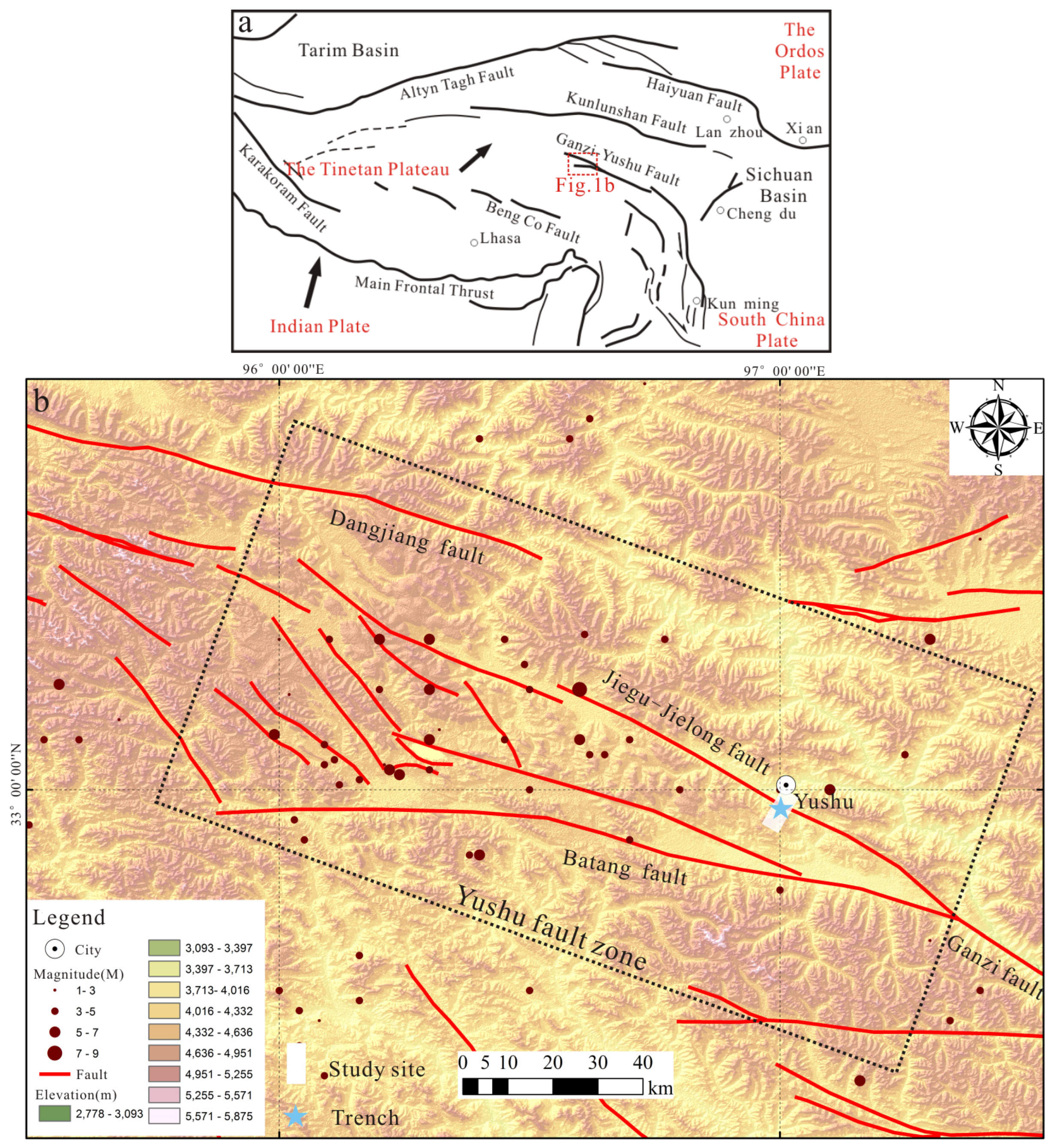
The Ganzi-Yushu fault is located at the boundary of the Qingtang and Bayan Har block in the central-eastern Tibetan Plateau and is part of the giant tectonic system (
Figure 1a) [
41,
49,
56,
57,
58]. Based on geomorphic features, the Ganzi-Yushu fault is commonly regarded as a sinistral strike-slip fault which was highly active in the Holocene. It is segmented into the Dangyang-Duocai fault, the Yushu fault and the Ganzi fault from northwest to southeast [
36,
38,
49,
50,
59,
60].
The Yushu fault, located in the neutral section of the Ganzi-Yushu fault, is mainly dominated by a sinistral-lateral strike-slip movement with a NW trending. The Yushu fault can be traced on remote sensing images ~150 km long from the northwest of Dangjiang city to the southeast of Yushu city (
Figure 1b). Geomorphologic features clearly show hints of its fault activity, such as triangular facets, pull-apart basins, river offsets and sag ponds, and so on [
57,
61,
62,
63,
64]. At least three earthquakes (Ms ≥ 6.5) have occurred on the Yushu fault and adjacent areas: the 1738 Ms 6.5 earthquake in the northwest of Yushu city (the location and intensity are still being disputed); the destructive 1896 Ms 7.0 earthquake in Shiqu city, and a powerful Ms 7.1 Yushu earthquake in 2010, causing serious damage. In respect of the geomorphic features and fault activity, the Yushu fault can be divided into three faults: Dangjiang, Jiegu-Jielong and Batang (
Figure 1b). Moreover, a series of secondary faults have also been found in the adjacent areas of these main segment faults.
The study site was situated in the vicinity of Minzhu village, Jiegu town (32.9882°N, 92.9998°E) with a ~3790 m elevation (
Figure 1b). From the geomorphic map of the study site as shown in
Figure 2, a groove landscape is distinctly discernible and was commonly considered to be the result of fault activity. There are a series of fault scarps with the height of ~20–30 cm at the flanks of the groove landscape (red arrows in
Figure 2b–e). The geomorphological and geological features are well preserved without a high degree of sedimentation and erosion from the field investigation. This area offers an ideal laboratory to capture high-precision topographic data and subsurface structures of active faults using TLS and multi-frequency GPR surveys. In addition, a trench had been dug by a previous researcher on the north edge of the groove landscape (
Figure 2b), and this provided useful subsurface information for GPR data interpretation. GPR surveys with different frequency antennas were conducted perpendicular to surface expressions of the active fault as shown in
Figure 2a,b. All GPR survey lines were paralleled to the western trench wall which allowed us to compare both datasets and interpret GPR images using the trench wall. The detailed shallow geometry of active faults was identified and analyzed by a combination of multi-frequency GPR profiles and trenching sections.
3. Materials and Methods
3.1. TLS Survey
The Stonex X300 terrestrial laser scanner was used to collect high-resolution geomorphic information as shown in
Figure 3a. This pulse-based scanner permits a massive collection of dense point clouds with a precision of ±5 mm at a range of 50 m. Maximum velocity reaches up to 60,000 points/s with an effective range of 300 m, and time consumption of one scanning station was not to exceed 10 min. The additional RGB information was gathered by an 8Mpix HDR camera integrated into the scanner to provide texture maps to point clouds. This terrestrial laser scanner was suitable for recording high-resolution geomorphic data on the Tibetan Plateau due to its high integration and easy operation.
In order to minimize the number of scanning positions and avoid possible omissions, four scanning positions were planned to perform at the study site with a wide horizontal and vertical view, and the adjacent scanning positions at a distance of ~50–80 m. Three spherical reflectors were used as the control points to combine multiple-station data into a unitary dataset (
Figure 3a). In addition, a Trimble R5 GPS antenna was mounted on top of the TLS to record geographical information received by the serial com-port on the GPS signal receivers. Once the point clouds were georeferenced in a real word co-ordinate system, it is easy to conduct a geometrical co-registration of TLS data and other spatial data.
With the aid of spherical reflector targets, Si-Scan software was used for combining the point clouds of four scanning positions to a unitary dataset (
Figure 3b). Subsequently, the raw point clouds were filtered using Geomagic Studio software to remove noise points such as power lines, vegetation and people, etc. to improve the signal-to-noise ratio. Finally, a resampling algorithm was chosen to minimize the number of point clouds and still maintain enough detailed information.
3.2. GPR Survey
GPR has proved to be an effective geophysical technology for depicting the shallow geometry of active faults utilizing dielectric contrasts in different media [
65]. Originally, GPR systems recorded and displayed continuous single-channel reflection waves on the 2D radargram. In this study, the RAMAC system of MALA Geosciences was chosen to gather the shallow geometry of active faults, which are oriented perpendicular to fault scarps as shown in
Figure 2b. The GPR system, equipped with 25 MHz and 100 MHz rough terrain antennas (RTA), and 250 MHz and 500 MHz shielded antennas, was implemented to image the shallow geometry of active faults at different depths and spatial resolutions.
Table 1 reports the locations of GPR profiles and parameter settings of different frequency GPR antennas.
A combination of GPR and differential GPS (DGPS) was carried out to obtain the shallow geometry of active faults with geographical coordinates and this provided accurate locations to each trace of GPR data (
Figure 4). The GPR system with 25 MHz and 100 MHz RTA antenna was connected to a Trimble R7 (RTK-GPS) signal receiver to delineate a sketch map of the shallow geometry of active faults. Subject to the rope shape of RTA antenna, the GPS antenna was fixed on the side of the backpack and the GPR data were recorded using the keyboard mode (
Figure 4b). Owing to the measurement points of GPR antenna and GPS antenna being separated, the GPR data had to be well matched with the positioning information of the GPS-RTK system when data collection was complete. To show more detailed shallow geometry of active faults with a better lateral and vertical resolution, high frequency antennas (250 MHz and 500 MHz) equipped with RTK-GPS were used along the 100 MHz GPR survey line (Line 3, 4 in
Figure 2a,b). In contrast to RTA antenna, the GPS antenna was mounted on the middle portion of the shielded antennas as shown in
Figure 4c. When the survey wheel of the GPR system was pulled at the surface, the GPR profile and its positioning information were obtained by the GPR system and GPS signal receiver at the same time [
66,
67].
Different filters were employed using ReflexW 7.2 software to reduce unwanted noise so as to improve the signal-to-noise ratio. The data processing steps are shown in
Table 2. After removing the invalid trace data, a subtract-DC-shift filter was applied to decrease the continuous or very low-frequency components of the GPR data. Then, zero timing of 5.5 ns, 11.5 ns, 43 ns and 117 ns were performed on 500 MHz, 250 MHz, 100 MHz and 25 MHz GPR profiles to redefine the real starting time of air/ground waves using time-zero correction. As the electromagnetic energy of the receiver signals will be attenuated, the GPR signals on each trace data can be amplified using energy decay. A background removal filter was employed to suppress the low-frequency noise and flat-lying reflectors. Cut-off frequencies of 10–40 MHz, 30–150 MHz, 180–600 MHz and 200–700 MHz were selected to eliminate noise signals on the 25 MHz, 100 MHz, 250 MHz and 500 MHz GPR data by band-pass filtering. The background noise and the antenna ringing signals were suppressed by running average filtering. Based on the known depth of the trench section, the average velocity of ~0.07 m/ns was calculated for time-depth conversion and Stolt migration. Finally, topographic correction was implemented to image the real subsurface structures using the high-resolution topographic data which had been acquired by the GPS-RTK system.
3.3. Trenching
Trenching is a powerful geological method for imaging stratigraphic units in the shallow subsurface, and has been widely applied in paleoseismology studies to reveal the paleoseismic history and seismogenic tendency of active faults [
68]. The fault history and the movements can be reconstructed by comprehensive analysis of stratigraphic units exposed in trench loggings. Based on geomorphologic evidence and field investigation at the study site, a ~12 m length and ~2 m depth trench had been excavated by previous researchers on the north edge of the groove landscape, which crosses the fault scarps as shown in
Figure 2b and
Figure 5. Stratigraphic units are distinctly different on each side of the fault scarps (
Figure 5). The trench section was used to reveal the stratigraphic units in shallow subsurface and it also provided useful information for better interpreting and analyzing the shallow geometry of active faults in the GPR data.
4. Results
4.1. TLS Results
The 3D point clouds, gathered by a Stonex X300 terrestrial laser scanner, are shown in
Figure 3b. The four circle blank areas represent TLS scanning positions, and do not affect the 3D reconstruction of geomorphic features. In general, the geomorphic features of active faults were difficult to observe in the scattered point clouds. In contrast to the scattered point clouds, a digital elevation model (DEM) provides more detailed topographic information to identify and analyze the geomorphic features of active faults. In this work, a DEM with a spatial resolution of 0.1 m was conducted on the filtered point clouds using Geomagic Studio software, as shown in
Figure 6a. Geomorphic features were well preserved without a high degree of sedimentation and erosion, and there were obvious topographic changes on DEM. The middle portion was dominated by the relatively lower elevation, while two flanks were characterized by the higher elevation, which were linked to fault scraps at the surface. This morphologic feature was supposed to be the typical groove landscape which resulted in fault activity. To show more detailed geomorphic features, ArcGIS software was used to create a surface slope map (as displayed in
Figure 6b). There were pronounced changes on the surface slope map and it was almost perfectly aligned with fault scarps at the surface. On the surface slope map, green represents a lower surface dip angle of ~0–9° and red indicates a higher surface dip angle of ~15°–68°. As a result, the interfaces of the low surface dip angle and high surface dip angle were regarded as faults F
1 and F
2 (red dotted lines in
Figure 6b).
Figure 6c shows the detailed 3D surficial model of the study site which was created by point clouds via the Golden Software Surfer 16. Geomorphic features on the detailed 3D surficial model were well matched with the results of the DEM and the surface slope map.
4.2. GPR Results
When a GPR antenna was employed across active faults, a remarkable variation of radar waves was exhibited on the GPR data by dielectric permittivity contrast in the surrounding medium. Generally, the fault and the associated structures were interpreted by the reflection pattern of electromagnetic wave as follows [
18,
19,
20,
21,
22,
25,
69,
70,
71,
72,
73]: (1) the continuous horizontal reflections of electromagnetic waves were interrupted or flexed; (2) diffraction hyperbolas or multiple reflection waves exist on two flanks of the fault; (3) the deformation zone of radar waves shows abrupt variations in them.
4.2.1. 25 MHz GPR Result
On the processed 25 MHz GPR data along SW–NE trending survey line (line 1 in
Figure 2a,b), a general skeleton map of shallow geometry with ~140 m long and ~60 m depth is displayed in
Figure 7. Topographic data of the 25 MHz GPR survey line is shown in
Figure 7a, and a groove landscape clearly found by topographic changes. Based on the radar reflection features of active faults, the shallow geometry of active faults were identified and interpreted as shown in
Figure 7b,c. There is an obvious boundary of strong energy reflections and weak energy reflections at the horizontal distance of ~78 m. On the left of the GPR profile (0–78 m), the reflection pattern of radar waves is characterized by relative regular reflections with strong energy reflections from top to bottom, implying homogeneous mediums in the subsurface. The right (~78–140 m) is mainly dominated by weak energy reflections related to heterogeneous media.
Two deformation zones with high-amplitude radar reflections are clearly distinguished between ~78 and ~140 m in
Figure 7b,c. At a distance of ~78–92 m and a depth of 0–12 m, the geometry of the deformation zone is wedge-shaped with a SW trending. Moreover, the continuous horizontal reflections of the radar waves were interrupted and there is flexure at ~78 and ~92 m. These remarkable variations of the radar waveform are considered to be the signature of fault activity. Between the distances of ~120–140 m, the deformation zone of the radar waves was dominated by strong irregular reflections with a NE trending, which was opposite to the trending of the continuous radar reflections between ~78 to 92 m.
To sum up, the deformation zone on the 25 MHz GPR image (~78–120 m) is inferred as the narrow fault system [
74,
75] and is almost perfectly consistent with topographic data as shown in
Figure 7a. Furthermore, the junctions of strong energy reflections and weak energy reflections at ~78 m, ~92 m and ~120 m are supposed to be the faults F
1, F
3 and F
2 (red dotted lines in
Figure 7c). The locations of faults F
1 and F
2 on the GPR profiles showed good consistency with the geomorphologic marks in
Figure 7a. Faults F
1 and F
2 are regarded as the boundary faults and the fault F
3 supposed to be the secondary fault.
4.2.2. Results—100 MHz, 250 MHz and 500 MHz GPR
The general view of shallow geometry of active faults was well depicted on the 25 MHz radar graph as shown in
Figure 7b,c. In order to image a more detailed shallow geometry of the narrow fault system on the 25 MHz GPR image (~78–120 m), GPR investigations with 100 MHz, 250 MHz and 500 MHz antenna were conducted oriented perpendicular to surface expression of active faults along survey lines 2, 3 and 4 (
Figure 2b).
Figure 8a represents the topographic data of the 100 MHz GPR measuring line. The shallow geometry of the deformation zone on the 25 MHz GPR data (~78–120 m) is presented on the 100 MHz GPR data with a maximum depth of ~16 m (
Figure 8b). In terms of the pronounced waveform and amplitude variations of radar waves, a deformation zone is easily discerned between the distance of ~12–58 m in
Figure 8b,c. At a distance of ~12 m and ~58 m, the distinct junctions of the strong radar reflections and low radar reflections are inferred as faults F
1 and F
2. Nevertheless, compared with 25 MHz GPR data, the interface of strong radar reflections and low radar reflections at a distance of ~30 m was ambiguous and the F
3 was not clearly identified. The reason for this appears to be that the 100 MHz GPR antenna might have been affected by external environmental factors or multiple reflections of electromagnetic waves when the GPR system was working. These interpreted results are well matched to the 25 MHz GPR interpreted image, and faults F
1 and F
2 show a good spatial correction with the location of geomorphic marks at the surface (
Figure 4c and
Figure 8a).
In contrast with low-frequency GPR antenna, the 250 MHz and 500 MHz GPR antenna are commonly adopted to depict the shallow geometry of active faults with high-resolution lateral and vertical resolution.
Figure 9a illustrates topographic data of the 250 MHz and 500 MHz GPR survey lines (line 3 and 4 in
Figure 2b), which is almost perfectly aligned with the location of the faults, F
1 and F
2. From the interpreted GPR results in
Figure 9b,c, the deformation zone and faults F
1, F
2 and F
3 are clearly distinguished by the remarkable variation of the radar waves, especially on the 500 MHz GPR image. At the horizontal distances of ~12–36 m, the reflection pattern of radar waves was mainly characterized by strong energy reflections with relatively regular waveforms. Between the distance of ~36–64 m, the upper part of 0~1 m depth was characterized by strong energy reflections, while weak energy reflections were found at a depth of ~1–2.5 m. As a consequence, the remarkable variations of the radar reflection were considered as the interfaces of stratigraphic units (black dotted lines in
Figure 9c). In addition, distortion and deformation zones with strong irregular energy reflections were seen at the distance of ~64–70 m and ~2.5 m in depth, which hints at sharp lithological contrasts.
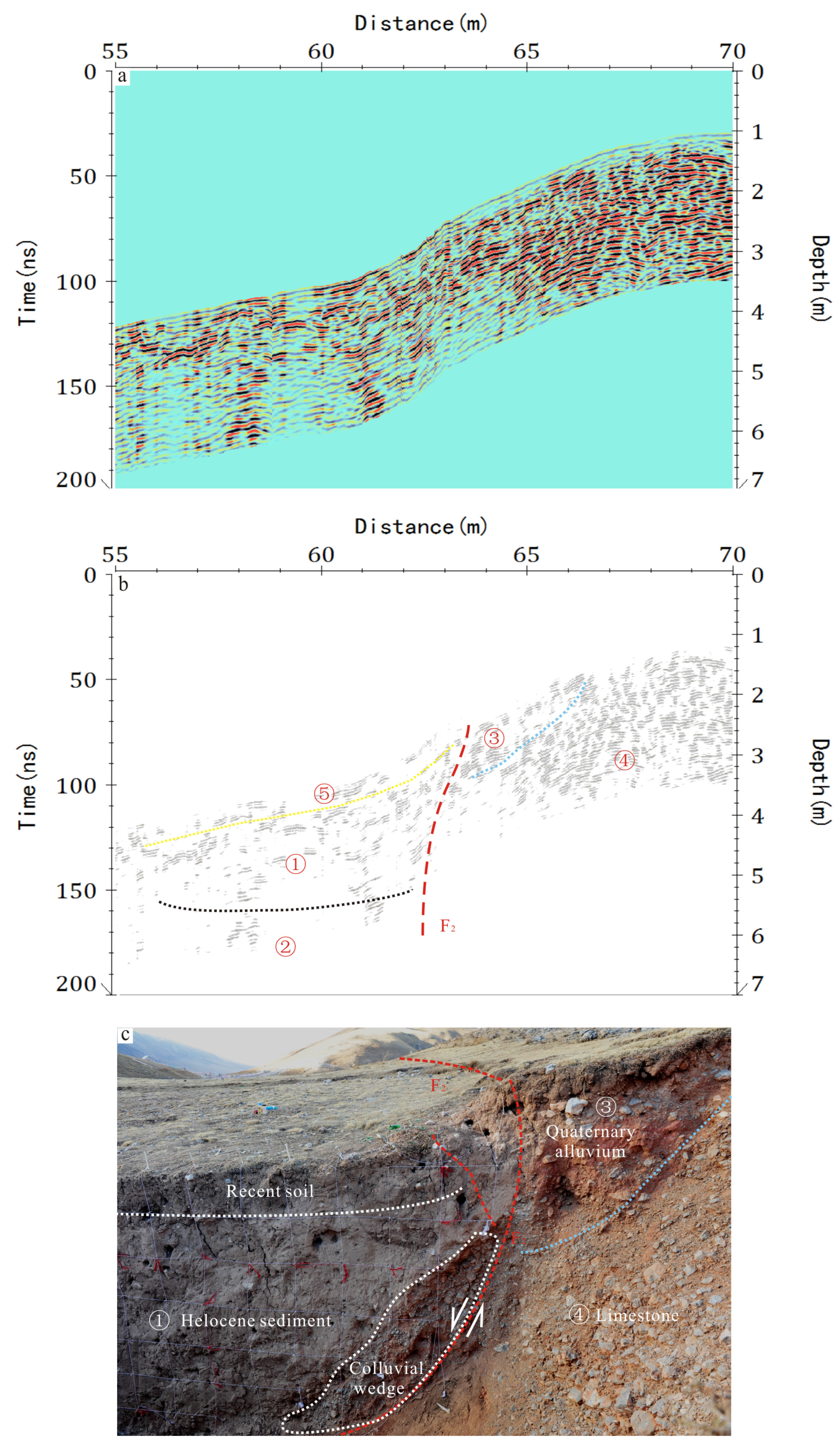
4.3. Trenching Section
Figure 10a shows the processed 500 MHz GPR data (the distances of ~55 m to 70 m in
Figure 9c).
Figure 10b is the interpreted 500 MHz GPR data, and
Figure 10c shows the western section of the trench (white rectangular box in
Figure 5b). Four stratigraphic units were seen on the trench section consisting of recent soil, Holocene sediment, Quaternary alluvium and limestone, and identified by white and blue dotted lines as shown in
Figure 10c. The upper stratigraphic unit consists of recent soil of ~25 cm thick with high water-saturated clay. In view of the sharp variation of radar waves, this stratigraphic unit was easily observed on the 500 MHz GPR profile (yellow dotted lines in
Figure 10b). The stratigraphic unit beneath the recent soil consisted of grey homogeneous sediments with a fine clay material, which is considered to be the result of fault activity (
Figure 2b). The flanks of the Holocene sediments were perfectly aligned with geomorphologic marks of faults F
1 and F
2 at the surface (
Figure 2b and
Figure 6). Holocene sediment was characterized by strong energy reflections with relative regular waveforms on the 500 MHz GPR data (the narrow fault system in
Figure 7,
Figure 8 and
Figure 9). In contrast to the fine material in sediment deposits, the orange unit was considered to be the Quaternary alluvium with some gravel scattered inside it, which is well aligned with relative moderate amplitude reflections. The stratigraphic unit at the bottom of the right portion of the trench, was dominated by limestone with many scattered centimetric stones. Considering the sharp lithological contrast between Quaternary alluvium and limestone, the prominent contacts of strong energy radar reflections and weak energy radar reflections were distinctly discernible on the 500 MHz GPR data. Moreover, the remarkable change of the radar reflections at a distance of ~64 m is regarded as fault F
2, which is almost perfectly matched with the colluvial wedge of trench section. The detailed logging of the trench, despite the limited investigation depth (~2 m), was consistent with the 500 MHz GPR result, while it was impossible to provide the subsurface information as deep as the 25 MHz, 100 MHz, 250 MHz and 500 MHz GPR images.
Although some stratigraphic units on trench section were not observed as deep as GPR data, the trench wall exhibited good consistency with the shallow geometry of different frequencies GPR profiles, especially on the 500 MHz radar graphs. In contrast to 25 MHz, 100 MHz and 250 MHz GPR results, the interface of strong radar reflections and low radar reflections was pretty obvious on the 500 MHz GPR data and thus it was inferred as fault F2. Due to strong lithological contrasts on the side of the fault, the waveform and amplitude of radar signals will change when the GPR antenna crosses it. Furthermore, the trending of the continuous horizontal reflections in the Holocene sediment was opposite to the radar reflections in the limestone. Nevertheless, owing to multiple materials in the fault zone, the fine structure of colluvial wedge was difficult to distinguish on the 500 MHz GPR image. To sum up, the 500 MHz GPR data is capable of imaging the detailed shallow geometry of stratigraphic units for understanding the fault kinematics and characteristics, such as location, dipping and direction of the fault. It will be gradually used for determining a suitable trench site for a paleoseismology study in Yushu area. When the survey depth requirement is not particularly high, stratigraphic units can be obtained by the 500 MHz GPR antenna instead of trench excavation, especially on the Tibetan Plateau with its diverse and fragile natural environment.
4.4. 3D Surficial and Subsurface Model
To better understand and analyze the fault kinematics and characteristics, a 3D surficial and subsurface model of the study site was produced using the Golden Software Surfer 16 based on TLS-derived data and GPR results as illustrated in
Figure 11.
Figure 11a,b shows the integration of 3D surficial model and GPR profile (25 MHz and 500 MHz), and the 3D surficial and subsurface model is displayed in
Figure 11c. The 25 MHz GPR data has a much better quality than other frequency GPR profiles, by providing a general view of shallow geometry of active faults with a ~60 m depth; while the 500 MHz GPR data was used to provide a better lateral and vertical resolution. Accordingly, the 25 MHz and 500 MHz GPR data were adapted to accurately register the 3D surficial model with the help of ground control points. In
Figure 11a,b, the interpreted GPR image shows three faults in the shallow subsurface, faults F
1 and F
3 dipping toward the NE and fault F
2 dipping towards the SW. In
Figure 11c, the 3D surficial and subsurface model confirms this interpretation with the trench observations, which provide additional information for a more comprehensive interpretation and analysis of the fault kinematics and characteristics.
The 3D surficial and subsurface model has the capability of providing multi-sensors and multi-view spatial data to characterize and understand the geomorphic features and shallow geometry of active faults. In addition, the shallow geometry of active faults in the GPR results can be better interpreted, depending on the corresponding surficial data. In the 3D surficial and subsurface model, the geomorphologic features were well preserved and identified by topographic changes. The typical groove landscape was situated in the middle portion as the result of fault activity. Many fault scarps with a height of ~20–30 cm were also identified at two flanks. A narrow fault system with ~40 m width and ~60 m depth was observed at the study site and exhibited a good spatial correlation with the typical groove landscape. Three faults were distinguished in the narrow fault system with faults F1 and F2 considered to be the boundary faults, while fault F3 was supposed to be the secondary fault. This interpreted result was also confirmed by geomorphic results of the TLS-derived data. In addition, the locations of the fault on the GPR profiles were almost perfectly aligned with topographic changes on the 3D surficial model of the TLS-derived data. The dipping directions of the fault were also determined by fault scarps at the surface.
Based on remote sensing image and field investigations, there were many geomorphologic features on the Yushu fault, such as triangular facets, pull-apart basins, river offsets and sag ponds, etc. These geomorphic features all indicate that the Yushu fault is mainly dominated by a sinistral-lateral strike-slip fault movement. Previous studies have suggested that the Jiegu-Jielong fault is a sinistral-lateral strike-slip fault with a normal component [
35,
36,
42,
44,
63,
64]. The typical groove landscape of the study site revealed that the fault was dominated by the strike-slip movement. From the GPR results and the trench observation, faults F
1 and F
2 were inferred as strike-slip faults with a normal component, as described in
Figure 11c.
5. Discussion
5.1. Muti-Frequency GPR Surveys
The detection depth of electromagnetic waves mainly relies on dielectric properties of the medium and antenna frequency [
65]. A high-frequency antenna has the advantage of providing a greater resolution at the expense of the lesser investigation depth, as the radar wave’s attenuation will be increased as the penetration deepens. Due to complex geological environments in the Yushu area, the investigation depths of 25 MHz, 100 MHz, 250 MHz and 500 MHz GPR antennas were all relatively lower than the theoretical detection depth, which varied from ~2.5 m to 60 m. Needless to say, the 250 MHz and 500 MHz radar graphs will offer a higher resolution in an investigation depicting the shallow geometry of active faults, than 25 MHz and 100 MHz GPR profiles. Nevertheless, the 25 MHz GPR profile has a much better quality than other frequencies GPR data when the medium has a high moisture content. The general view of the shallow geometry of active faults was well presented on the 25 MHz GPR image at a ~60 m depth. Moreover, the faults (F
1, F
2 and F
3) and their features, such as location, dipping and direction, were also clearly identified and interpreted on the 25 MHz GPR data. For the sake of revealing more detailed shallow geometry, GPR investigations with 100 MHz, 250 MHz and 500 MHz antennas were used to obtain abundant information on the narrow fault system. The interfaces of stratigraphic units were easily found on the high-resolution GPR profiles by means of the remarkable variations of the radar wave’s signals, especially on the 500 MHz GPR data.
GPR surveys with 500 MHz shielded antenna were first used to image the shallow geometry of the Yushu fault in 2015. A comparison between GPR images and trench walls was performed in four study sites along the Yushu fault. Zhang et al. (2015) illustrated that GPR is capable of detecting stratigraphic units in the Yushu area which has an extreme natural environment [
54]. Compared with the single frequency GPR survey on the Yushu strike-slip fault or other strike-slip faults around the world [
54,
76,
77,
78], a multi-frequency GPR profile has the great advantage of imaging the detailed shallow geometry of active faults at different depths and spatial resolutions to improve the interpreted results. The 25 MHz GPR profile has a much better quality than other frequency GPR data in the Yushu area. In addition, when geological environment is complex, either a trench excavation or a borehole is still needed to provide useful information to better interpret the shallow geometry of active faults on the GPR data.
As a whole, multi-frequency GPR antennas are capable of providing more detailed information for interpreting and understanding the shallow geometry of active faults. This case study strongly supports the use of multi-frequency GPR antennas to image the shallow geometry of the Yushu fault, especially on the Tibetan Plateau with its harsh natural environment. Considering the geological condition of the Yushu area and different frequency’s GPR results, the GPR measurement with 25 MHz and 500 MHz antennas are particularly suitable for characterizing the shallow geometry of the Yushu fault.
5.2. The Combination of TLS and GPR Methods
It is challenging to obtain detailed topographic data and shallow geometry of active faults by conventional methods, especially on the Tibetan Plateau with its high altitudes and risk of hypoxia. A combination of TLS and GPR methods has been commonly applied to obtain the geomorphic information and shallow geometry of active faults in a non-destructive and cost-effective way. The combination of these methods provides multi-sensors and multi-view spatial data to achieve a more comprehensive understanding and interpretation of active faults. Furthermore, the shallow geometry of active faults on the GPR results can be better understood with the aid of the corresponding surficial data [
27,
28,
29,
30,
31,
32,
33].
TLS is typically adopted to acquire high-precision topographic information to reconstruct a detailed 3D realistic surface model of active faults. A deformation area in the lower elevation, paralleling to surface traces of active faults, was well observed on the TLS-derived data. It was considered to be a typical groove landscape resulting from fault activity (
Figure 6). However, buried structures of active faults were not detected by TLS, and subsurface data is essential to comprehensively understand and interpret the fault’s kinematics and characteristics with its corresponding surficial data. Hence, GPR surveys with different frequency antennas were conducted to investigate the shallow geometry of active faults along the survey lines in
Figure 2a,b. The general view of the shallow geometry of active faults was well depicted on the 25 MHz GPR image (
Figure 7). In addition, a deformation zone of radar waves with ~40 m width and ~60 m depth was easily distinguished in the 25 MHz GPR result, and its geometry was wedge-shaped with a SW trending (
Figure 7b,c). In order to show more detailed shallow geometry of the defamation zone, the 100 MHz, 250 MHz and 500 MHz GPR data were obtained along the survey lines 2, 3 and 4 (
Figure 2a,b). The 100 MHz, 250 MHz and 500 MHz GPR interpreted results were well matched with the 25 MHz GPR interpreted profile. The deformation zone between the faults F
1 and F
2 was inferred as the narrow fault system, and it was almost perfectly aligned with topographic data as displayed in
Figure 7a,
Figure 8a and
Figure 9a. Three faults were found on the narrow fault system, with faults F
1 and F
2 considered to be the boundary faults, while fault F
3 was supposed to be the secondary fault (
Figure 7c,
Figure 8c and
Figure 9c).
The multi-frequency GPR interpreted results exhibited good consistency with geomorphic marks of the TLS-derived data. Although some stratigraphic units on the trench wall were not found to be as deep as the GPR data, the trench section was well matched with the 500 MHz GPR profile. In terms of the TLS, GPR results and the trench observation, the wedge-shaped deformation zone on different frequency GPR profiles was considered to be the narrow fault system, which is associated with the typical groove landscape at the surface. The faults F1 and F2 were regarded as strike-slip faults with a normal component.
6. Conclusions
The integrated TLS and multi-frequency GPR methods, in combination with trenching, were used to depict a detailed surficial and subsurface geometry of the Yushu fault. The 3D surficial and subsurface model has been constructed to achieve more comprehensive understanding and interpretation of the fault’s kinematics and characteristics. The conclusions of the study are described as follows:
(1) TLS is capable of obtaining a high-resolution and detailed 3D realistic model of geomorphic features. A deformation area with the lower elevation, paralleling to surface traces of active faults, was well observed on the TLS-derived data and was considered to be a typical groove landscape resulting from fault activity.
(2) Multi-frequency GPR antennas (25 MHz, 100 MHz, 250 MHz and 500 MHz) were used to reveal the shallow geometry of active faults in a non-invasive and low-cost way. A narrow fault system with ~40 m width and ~60 m depth was observed and exhibited a good spatial correlation with the typical groove landscape at the surface. Three faults were found on the narrow fault system and faults F1 and F2 were considered to be the boundary faults, while fault F3 was supposed to be the secondary fault. In addition, the GPR system with the 25 MHz and 500 MHz antennas are particularly suitable for characterizing the shallow geometry of the Yushu fault.
(3) Although some stratigraphic units on the trench section were not found as deep as the GPR profiles, the trench wall exhibited good consistency with the shallow geometry of the 500 MHz data. This will be gradually used for determining a suitable trench site for a paleoseismology study in the Yushu area, and stratigraphic units can be obtained by the 500 MHz GPR antenna instead of the trench excavation when the survey depth requirement is not particularly high.
(4) The 3D surficial and subsurface model provides multi-sensors and multi-view spatial data for characterizing and understanding the geomorphic features and shallow geometry of active faults. Shallow geometry of active faults on the GPR results can be better understood by the corresponding surficial data. The typical groove landscape of the study site was dominated by a sinistral-lateral strike-slip fault and faults F1 and F2 were inferred as the strike-slip faults with a normal component.
This study demonstrated that a combination of TLS, multi-frequency GPR and trenching was suitable to characterize a detailed surficial and subsurface geometry of the Yushu fault. When geological environment is complex, trench excavation or a borehole is still needed to provide useful information to better interpret the shallow geometry of active faults on the GPR data. In addition, the integration of GPR and other remote sensing methods or geophysical prospecting will be gradually used for active faults investigation and seismic hazard assessment, such as UAV, LiDAR, electrical resistivity tomography (ERT), spontaneous potential (SP), active and passive seismic surveys, and so on.
Author Contributions
Methodology, D.Z., J.L., Z.W. and L.R.; investigation, D.Z. and J.L.; writing—original draft preparation, D.Z. and J.L.; writing—review and editing, J.L., Z.W. and L.R.; data processing and interpretation, D.Z., J.L., Z.W. and L.R.; supervision, J.L.; project administration, J.L.; funding acquisition, Z.W. and D.Z. All authors have read and agreed to the published version of the manuscript.
Funding
This research was funded by the National Natural Science Foundation of China (NO: U2002211), the China Geology Survey project (NO: DD20221644), China Postdoctoral Science Foundation (No. 2020M680606), Beijing Postdoctoral Research Foundation, the Science and Technique Foundation of Henan Province (No. 222102320155, 212102310427) and the Key scientific research Foundation of the university in Henan Province (No. 22A420003, 21A420002).
Data Availability Statement
The data presented in this study are available on request from the corresponding author.
Acknowledgments
We thank Ma Xiaoxue and Li Kai for assistance with the field investigation, TLS and GPR data acquirement in the Yushu area.
Conflicts of Interest
The authors declare no conflict of interest.
Correction Statement
This article has been republished with a minor correction in this article’s reference 75. This change does not affect the scientific content of the article.
References
- Hooper, D.M.; Bursik, M.I.; Webb, F.H. Application of high-resolution, interferometric DEMs to geomorphologic studies of fault scarps, Fish Lake Valley, Nevada-California, USA. Remote Sens. Environ. 2003, 84, 255–267. [Google Scholar] [CrossRef]
- Arrowsmith, J.R.; Zielke, O. Tectonic geomorphology of the San Andreas Fault zone from high resolution topography: An example from the Cholame segment. Geomorphology 2009, 113, 70–81. [Google Scholar] [CrossRef]
- Liu, J.; Chen, T.; Zhang, P.; Zhang, H.; Zheng, W.; Ren, Z.; Liang, S.; Sheng, C.; Gan, W. Illuminating the active Haiyuan fault, China by Airborne Light Detection and Ranging. Chin. Sci. Bull. 2013, 58, 41–45. [Google Scholar]
- Maruyama, T.; Lin, A. Active strike-slip faulting history inferred from offsets of topographic features and basement rocks: A case study of the Arima–Takatsuki Tectonic Line, southwest Japan. Tectonophysics 2002, 344, 81–101. [Google Scholar] [CrossRef]
- Deng, Q.; Chen, L.; Ran, Y. Quantitative studies and applications of active tectonic. Earth Sci. Front. 2004, 11, 383–392. [Google Scholar]
- Zhang, P.; Deng, Q.; Zhang, Z.; Li, H. Active faults, earthquake hazards and associated geodynamic processes in continental China. Sci. Sin. Terra 2013, 43, 1607–1620. [Google Scholar]
- Papanikolaou, L.D.; Balen, R.V.; Silva, P.G.; Reicherter, K. Geomorphology of active faulting and seismic hazard assessment: New tools and future challenges. Geomorphology 2015, 237, 1–13. [Google Scholar] [CrossRef]
- Ren, Z.; Zielke, O.; Yu, J. Active tectonics in 4D high-resolution. J. Struct. Geol. 2018, 117, 264–271. [Google Scholar] [CrossRef]
- Wu, Z. The Definition and Classification of Active faults: History, Current Status and Progress. Acta Geosci. Sin. 2019, 40, 661–697. [Google Scholar]
- Wu, Z. Active Faults and Engineering Applications Ⅰ: Definition and Classification. J. Earth Sci. Environ. 2022, 44, 922–947. [Google Scholar]
- Kayen, R.; Pack, R.T.; Bay, J.; Sugimoto, S.; Tanaka, H. Terrestrial-LIDAR Visualization of Surface and Structural Deformations of the 2004 Niigata Ken Chuetsu, Japan, Earthquake. Earthq. Spectra 2006, 22, 147–162. [Google Scholar] [CrossRef]
- Derron, M.H.; Jaboyedoff, M. Preface “LIDAR and DEM techniques for landslides monitoring and characterization”. Nat. Hazards Earth Syst. Sci. 2010, 10, 1877–1879. [Google Scholar] [CrossRef]
- Ma, H. Review on applications of LiDAR mapping technology to geosciences. Earth Sci. J. China Univ. Geosci. 2011, 36, 347–354. [Google Scholar]
- Gold, P.O.; Oskin, M.E.; Elliott, A.J.; Hinojosa-Corona, A.; Taylor, M.H.; Kreylos, O.; Cowgill, E. Coseismic slip variation assessed from terrestrial lidar scans of the El Mayor-Cucapah surface rupture. Earth Planet. Sci. Lett. 2013, 366, 151–162. [Google Scholar] [CrossRef]
- Ren, Z.; Chen, T.; Zhang, H.; Zheng, W.; Zhang, P. LiDAR Survey in Active Tectonics Studies:An Introduction and Overview. Acta Geol. Sin. 2014, 88, 1197–1202. [Google Scholar]
- Tang, Y.; Wei, S.; Song, J.; Zhang, D.; Zheng, W. Key technology and application of terrestrial LiDAR in 3D active faults model. Acta Sci. Nat. Univ. Sunyatseni 2021, 60, 78–87. [Google Scholar]
- Zhang, D.; Li, J.; Wu, Z.; Liu, S.; Lu, Y. Using terrestrial LiDAR to accurately measure the microgeomorphologic geometry of active faults: A case study of fault scarp on the Maoyababa fault zone. J. Geomech. 2021, 27, 63–72. [Google Scholar]
- Carbonel, D.; Rodríguez Tribaldos, V.; Gutiérrez, F.; Galve, J.P.; Guerrero, J.; Zarroca, M.; Roqué, C.; Linares, R.; Mccalpin, J.P.; Acosta, E. Investigating a damaging buried sinkhole cluster in an urban area (Zaragoza city, NE Spain) integrating multiple techniques: Geomorphological surveys, DInSAR, DEMs, GPR, ERT, and trenching. Geomorphology 2015, 229, 3–16. [Google Scholar] [CrossRef]
- Yalçıner, C.Ç.; Altunel, E.; Bano, M.; Meghraoui, M.; Karabacak, V.; Akyüz, H.S. Application of GPR to normal faults in the Buyuk Menderes Graben, western Turkey. J. Geodyn. 2013, 65, 218–227. [Google Scholar] [CrossRef]
- Dujardin, J.R.; Bano, M.; Schlupp, A.; Ferry, M.; Munkhuu, U.; Tsend-Ayush, N.; Enkhee, B. GPR measurements to assess the Emeelt active faults’s characteristics in a highly smooth topographic context, Mongolia. Geophys. J. Int. 2014, 198, 174–186. [Google Scholar] [CrossRef]
- Anchuela, Ó.P.; Lafuente, P.; Arlegui, L.; Liesa, C.L.; Simón, J.L. Geophysical characterization of buried active faults: The Concud Fault (Iberian Chain, NE Spain). Int. J. Earth Sci. 2016, 105, 2221–2239. [Google Scholar] [CrossRef]
- Maurya, D.; Chowksey, V.; Tiwari, P.; Chamyal, L. Tectonic geomorphology and neotectonic setting of the seismically active South Wagad Fault (SWF), Western India, using field and GPR data. Acta Geophys. 2017, 65, 1167–1184. [Google Scholar] [CrossRef]
- Lunina, O.V.; Gladkov, A.S.; Gladkov, A.A. Surface and shallow subsurface structure of the Middle Kedrovaya paleoseismic rupture zone in the Baikal Mountains from geomorphological and ground-penetrating radar investigations. Geomorphology 2019, 326, 54–67. [Google Scholar] [CrossRef]
- Nappi, R.; Paoletti, V.; D’Antonio, D.; Soldovieri, F.; Capozzoli, L.; Ludeno, G.; Porfido, S.; Michetti, A.M. Joint Interpretation of Geophysical Results and Geological Observations for Detecting Buried Active Faults: The Case of the “Il Lago” Plain (Pettoranello del Molise, Italy). Remote Sens. 2021, 13, 1555. [Google Scholar] [CrossRef]
- Ercoli, M.; Cirillo, D.; Pauselli, C.; Jol, H.M.; Brozzetti, F.J.C.G. Ground-penetrating radar signature of Quaternary faulting: A study from the Mt. Pollino region, southern Apennines, Italy. Solid Earth 2021, 12, 2573–2596. [Google Scholar] [CrossRef]
- Lazar, M.; Basson, U.; Ben-David, R.; Coddington, J. When faults diverge -High resolution imaging of an intra-fault zone in an urban environment. A case study from the city of Tiberias, Israel. Eng. Geol. 2022, 296, 106454. [Google Scholar] [CrossRef]
- Kayen, R.; Barnhardt, A.; Carkin, B.A.; Grossman, E.E.; Minasian, D.; Thompson, M. Imaging the M7.9 Denali Fault Earthquake 2002 rupture at the Delta River using LiDAR, RADAR, and SASW Surface Wave Geophysics. In Proceedings of the American Geophysical Union, Fall Meeting 2004, San Francisco, CA, USA, 9–13 December 2004. [Google Scholar]
- Zhang, D.; Wu, Z.; Li, C.; Liu, S.; Ma, D.; Lu, Y. The delineation of three-dimensional shallow geometry of active fault based on TLS and GPR: A case study of an normal fault on the north margin of Maoyaba Basin in Litang, Western Sichuan Province. Seismol. Geol. 2019, 41, 377–399. [Google Scholar]
- Bubeck, A.; Wilkinson, M.; Roberts, G.P.; Cowie, P.A.; McCaffrey, K.J.W.; Phillips, R.; Sammonds, P. The tectonic geomorphology of bedrock scarps on active normal faults in the Italian Apennines mapped using combined ground penetrating radar and terrestrial laser scanning. Geomorphology 2015, 237, 38–51. [Google Scholar] [CrossRef]
- Cowie, P.A.; Phillips, R.J.; Roberts, G.P.; McCaffrey, K.; Zijerveld, L.J.J.; Gregory, L.C.; Faure Walker, J.; Wedmore, L.N.J.; Dunai, T.J.; Binnie, S.A.; et al. Orogen-scale uplift in the central Italian Apennines drives episodic behaviour of earthquake faults. Sci. Rep. 2017, 7, 44858. [Google Scholar] [CrossRef]
- Spahic, D.; Exner, U.; Behm, M.; Grasemann, B.; Haring, A. Structural 3D modeling using GPR in unconsolidated sediments (Vienna basin, Austria). Trab. Geol. 2010, 29, 250–252. [Google Scholar]
- Schneiderwind, S.; Mason, J.; Wiatr, T.; Papanikolaou, I.; Reicherter, K. 3-D visualisation of palaeoseismic trench stratigraphy and trench logging using terrestrial remote sensing and GPR–A multiparametric interpretation. Solid Earth 2016, 7, 323–340. [Google Scholar] [CrossRef]
- Zhang, D.; Wu, Z.; Shi, D.; Li, J.; Lu, Y. Integration of Terrestrial Laser Scanner (TLS) and Ground Penetrating Radar (GPR) to Characterize the Three-Dimensional (3D) Geometry of the Maoyaba Segment of the Litang Fault, Southeastern Tibetan Plateau. Remote Sens 2022, 14, 6394. [Google Scholar] [CrossRef]
- Pan, J.; Li, H.; Wu, F. Surface rupture characteristics, rupture mechanics, and rupture process of the Yushu earthquake(Ms 7.1). Acta Petrol. Sin. 2011, 27, 3449–3459. [Google Scholar]
- Huang, X.; Jing, Z.; Xie, F.; Zhao, J. Late quaternary slip rate of the east segment of the Yushu fault in the central-eastern Tibetan Plateau. Quat. Int. 2019, 532, 146–156. [Google Scholar] [CrossRef]
- Chen, L.; Wang, H.; Rang, Y.; Sun, X.; Su, G.; Wang, G.; Tan, X.; Li, Z.; Zhang, X. The Ms7.1 Yushu earthquake surface ruptures and historical earthquakes. Chin. Sci. Bull. 2010, 55, 1200–1205. [Google Scholar]
- Zhang, Y.; Xu, L.; Chen, Y. Fast inversion of rupture process for 14 April 2010 Yushu, Qinghai, earthquake. Acta Geol. Sin. 2010, 23, 201–204. [Google Scholar] [CrossRef][Green Version]
- Xu, L.; Di, H.; Feng, W.; Li, C. Estimation of the fault-near ground motion of the 2010 Yushu, Qinghai, Ms7.1 earthquake. Chin. J. Geophys. 2010, 53, 1366–1373. [Google Scholar]
- Zhang, G.; Shan, X.; Delouis, B.; Qu, C.; Balestra, J.; Li, Z.; Liu, Y.; Zhang, G. Rupture history of the 2010 Ms7.1 Yushu earthquake by joint inversion of teleseismic data and InSAR measurements. Tectonophysics 2013, 584, 129–137. [Google Scholar] [CrossRef]
- Xu, X.; Wang, Y.; He, J. Research on central focal mechanism and its surrounding tectonic stress field of the Yushu MS7.1 earthquake in Qinghai. Plateau Earthq. Res. 2021, 33, 1–10. [Google Scholar]
- Qin, T.; Zhou, Y.; Zhang, P.Z. Along-strike variation in fault structural maturity and seismic moment deficits on the Yushu-Ganzi-Xianshuihe fault system revealed by strain accumulation and regional seismicity. Earth Planet. Sci. Lett. 2022, 596, 117799. [Google Scholar]
- Zhang, Y.; Ma, Y.; Hu, D.; Yang, N.; Xiong, T.; Guo, C. Investigation and Research on the Surface Rupture of the Yushu Earthquake and Reconstruction Site Selection. Acta Geol. Sin. 2010, 84, 593–605. [Google Scholar]
- Zhang, G.; Qu, C.; Shan, X.; Liu, Y.; Song, X. The surface rupture and coseismic deformation characteristics of MS 7.1 earthquake at Qinghai Yushu in 2010. Chin. J. Geophys. 2011, 54, 121–127. [Google Scholar]
- Lin, A.; Rao, G.; Jia, D.; Wu, X.; Yan, B.; Ren, Z. Co-seismic strike-slip surface rupture and displacement produced by the 2010 M W 6.9 Yushu earthquake, China, and implications for Tibetan tectonics. J. Geodyn. 2011, 52, 249–259. [Google Scholar] [CrossRef]
- Lin, A.; Jia, D.; Rao, G.; Yan, B.; Wu, X.; Ren, Z. Recurrent Morphogenic Earthquakes in the Past Millennium along the Strike-Slip Yushu Fault, Central Tibetan Plateau. Bull. Seismol. Soc. Am. 2011, 101, 2755–2764. [Google Scholar] [CrossRef]
- Zhou, C.; Wu, Z.; Nima, C.; Li, J.; Jiang, Y.; Liu, Y. Structural analysis of the co-seismic surface ruptures associated with the Yushu Ms7.1 earthquake, Qinghai Province. Geol. Bull. China 2014, 33, 551–566. [Google Scholar]
- Wu, J.; Huang, X.; Xie, F. Deformation of the Most Recent Co-seismic Surface Ruptures Along the Garzê–Yushu Fault Zone (Dangjiang Segment) and Tectonic Implications For the Tibetan Plateau. Acta Geol. Sin. Engl. Ed. 2017, 91, 443–454. [Google Scholar] [CrossRef]
- Ren, J.; Xie, F.; Liu, D.; Zhang, A. Study of Tectonics, Seismicity and Recurrence Interval of Yushu 2010 Earthquake, Qinghai Province. Technol. Earthq. Disaster Prev. 2010, 5, 228–233. [Google Scholar]
- Wu, Z.; Zhou, C.; Feng, H.; Zhang, K.; Li, J.; Ye, P.; Li, Y.; Tian, T. Active faults and earthquake around Yushu in eastern Tibetan Plateau. Geol. Bull. China 2014, 33, 419–469. [Google Scholar]
- Shi, F.; He, H.; Densmore, A.L.; Li, A.; Yang, X.; Xu, X. Active tectonics of the Ganzi–Yushu fault in the southeastern Tibetan Plateau. Tectonophysics 2016, 676, 112–124. [Google Scholar] [CrossRef]
- Zhao, N.; Ji, L.; Zhang, W.; Xu, X.; Wang, J. Present-day kinematics and seismic potential of the Ganzi-Yushu fault, eastern Tibetan plateau, constrained from InSAR. Front. Earth Sci. 2023, 11, 1123711. [Google Scholar] [CrossRef]
- Yuan, X.; Wang, X.; Dou, A.; Dong, Y.; Wang, L.; Jin, D. Terrestrial LiDAR-based 3D Modelling Analysis of Surface rupture caused by Yushu Earthquake. Seismol. Geol. 2010, 34, 39–46. [Google Scholar]
- Zhao, H.; Li, D.; Zhao, J.; Zhang, L.; Chen, X. Exploration for the Southern Segment of the Ganzi-Yushu Fault Zone Using Shallow Seismic Reflection Method. Earthq. Res. Sichuan 2021, 1, 6–11. [Google Scholar]
- Zhang, D.; Li, J.; Wu, Z.; Zhong, R.; Tian, T.; Zhang, D. Preliminary Application of Ground Penetrating Radar to Active Faults along Yushu Strike-Slip Faults Zone. Geol. Bull. China 2015, 34, 204–215. [Google Scholar]
- Zhang, D.; Li, J.; Liu, S.; Wang, G. Multi-frequencies GPR measurements for delineating the shallow subsurface features of the Yushu strike slip fault. Acta Geophys. 2019, 67, 501–515. [Google Scholar] [CrossRef]
- Wen, X.; Xu, X.; Zheng, R.; Xie, Y.; Wan, C. Average slip-rate and recent large earthquake ruptures along the Garzê-Yushu fault. Sci. China Earth Sci. 2003, 46, 276–288. [Google Scholar]
- Zhou, R.; Wen, X.; Chai, C.; Ma, S. Recent earthquakes and assessment of seismic tendency on the Ganzi-Yushu Fault zone. Seismol. Geol. 1997, 19, 115–124. [Google Scholar]
- Xu, X.; Wen, X.; Zheng, R.; Ma, W.; Song, F.; Yu, G. Pattern of latest tectonic motion and its dynamics for active blocks in Sichuan-Yunnan region, China. Sci. China 2003, 46, 210–226. [Google Scholar]
- Pei, S.; Chen, Y.; Feng, B.; Gao, X.; Su, J. High-resolution seismic velocity structure and azimuthal anisotropy around the 2010 Ms = 7.1 Yushu earthquake, Qinghai, China from 2D tomography. Tectonophysics 2013, 584, 144–151. [Google Scholar] [CrossRef]
- Zhou, R.; Ma, S.; Cai, C. Late quaternary active features of the Ganzi-Yushu fault zone. Earthq. Res. China 1996, 12, 250–260. [Google Scholar]
- Tian, T.; Wu, Z.; Gai, H.; Zhou, C.; Zhang, K.; Ma, Z. Dating of multi-period earthquake-triggered rockfalls: A method for revealing paleo-seismic events that occurred along the Yushu fault in the eastern Tibetan Plateau. Landslides 2022, 19, 351–371. [Google Scholar] [CrossRef]
- Zhang, G.; Shan, X.; Feng, G. The 3-D surface deformation, coseismic fault slip and after-slip of the 2010 M w 6.9 Yushu earthquake, Tibet, China. J. Asian Earth Sci. 2016, 124, 260–268. [Google Scholar] [CrossRef]
- Li, Y.; Wu, Z.; Ye, P.; Ma, D.; Liu, Y.; Jiang, Y.; Li, J.; Zhou, C. The geomorphologic and geological marks of the active left-lateral strike-slip fault and the characteristics of geometry and kinematics along the Yushu fault zone in southeastern Tibet. Geol. Bull. China 2013, 32, 1410–1422. [Google Scholar]
- Li, J.; Wu, Z.; Zhang, D.; Liu, X. Remote sensing image interpretation and tectonic activity study of the main active faults in Yushu area, Qinghai Province. Geol. Bull. China 2014, 33, 535–550. [Google Scholar]
- Jol, H.M. Ground Penetrating Radar: Theory and Applications; Elsevier Science: Kidlington, UK, 2009. [Google Scholar]
- Zhang, D.; Gong, H.; Wu, Z.; Liu, S. Integrated ground penetrating radar and DGPS method for the continuous and long-distance GPR survey in the rugged terrain. Acta Geophys. 2022, 70, 537–546. [Google Scholar] [CrossRef]
- Tanajewski, D.; Bakula, M. Application of Ground Penetrating Radar Surveys and GPS Surveys for Monitoring the Condition of Levees and Dykes. Acta Geophys. 2016, 64, 1093–1111. [Google Scholar] [CrossRef]
- Mccalpin, J.P. Field Techniques in Paleoseismology—Terrestrial Environments; Academic Press: San Diego, CA, USA, 2009; pp. 29–118. [Google Scholar]
- Busby, J.P.; Merritt, J.W. Quaternary deformation mapping with ground penetrating radar. J. Appl. Geophys. 1999, 41, 75–91. [Google Scholar] [CrossRef]
- McClymont, A.F.; Villamor, P.; Green, A.G. Assessing the contribution of off-fault deformation to slip-rate estimates within the Taupo Rift, New Zealand, using 3-D ground-penetrating radar surveying and trenching. Terra Nova 2009, 21, 446–451. [Google Scholar] [CrossRef]
- Maurya, D.M.; Chouksey, V.; Joshi, P.N.; Chamyal, L.S. Application of GPR for delineating the neotectonic setting and shallow subsurface nature of the seismically active Gedi fault, Kachchh, western India. J. Geophys. Eng. 2013, 10, 034006. [Google Scholar] [CrossRef]
- Lunina, O.V.; Gladkov, A.S.; Afonkin, A.M.; Serebryakov, E.V. Deformation style in the damage zone of the Mondy fault: GPR evidence (Tunka basin, southern East Siberia). Russ. Geol. Geophys. 2016, 57, 1269–1282. [Google Scholar] [CrossRef]
- Lei, X.; Ren, J.; Xu, X.; Qian, R.; Zhang, J.; Song, B. Application of high-power ground-penetrating radar antennas with different frequencies to quickly locate the upper breakpoint of active buried faults in an urban area in the Datong basin (northern China). J. Appl. Geophys. 2022, 196, 104515. [Google Scholar] [CrossRef]
- Van der Pluijm, B.A.; Marshak, S. Earth Structure—An Introduction to Structural Geology and Tectonics; W.W. Norton & Company Ltd.: New York, NY, USA; London, UK, 2004. [Google Scholar]
- Brandes, C.; Tanner, D. Fault Mechanics and Earthquakes. In Understanding Faults: Detecting, Dating, and Modeling; Tanner, D., Brandes, C., Eds.; Elsevier: Oxford, UK, 2020; pp. 11–80. [Google Scholar]
- Beauprêtre, S.; Garambois, S.; Manighetti, I.; Malavieille, J.; Sénéchal, G.; Chatton, M.; Davies, T.; Larroque, C.; Rousset, D.; Cotte, N.; et al. Finding the buried record of past earthquakes with GPR-based palaeoseismology: A case study on the Hope fault, New Zealand. Geophys. J. Int. 2012, 189, 73–100. [Google Scholar] [CrossRef]
- Carpentier, S.; Green, A.G.; Doetsch, J.; Dorn, C.; Kaiser, A.E.; Campbell, F.; Horstmeyer, H.; Finnemore, M. Recent deformation of Quaternary sediments as inferred from GPR images and shallow P-wave velocity tomograms: Northwest Canterbury Plains, New Zealand. J. Appl. Geophys. 2012, 81, 2–15. [Google Scholar] [CrossRef]
- Slater, L.; Niemi, T.M. Ground-penetrating radar investigation of active faults along the Dead Sea Transform and implications for seismic hazards within the city of Aqaba, Jordan-ScienceDirect. Tectonophysics 2003, 368, 33–50. [Google Scholar] [CrossRef]
| Disclaimer/Publisher’s Note: The statements, opinions and data contained in all publications are solely those of the individual author(s) and contributor(s) and not of MDPI and/or the editor(s). MDPI and/or the editor(s) disclaim responsibility for any injury to people or property resulting from any ideas, methods, instructions or products referred to in the content. |
© 2023 by the authors. Licensee MDPI, Basel, Switzerland. This article is an open access article distributed under the terms and conditions of the Creative Commons Attribution (CC BY) license (https://creativecommons.org/licenses/by/4.0/).


