
TEC Anomalies Detection for Qinghai and Yunnan Earthquakes on 21 May 2021

 , ,
, ,  , and
, and
Abstract
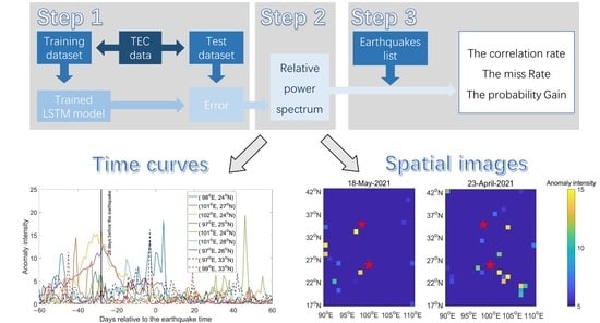
1. Introduction
2. Materials and Methods
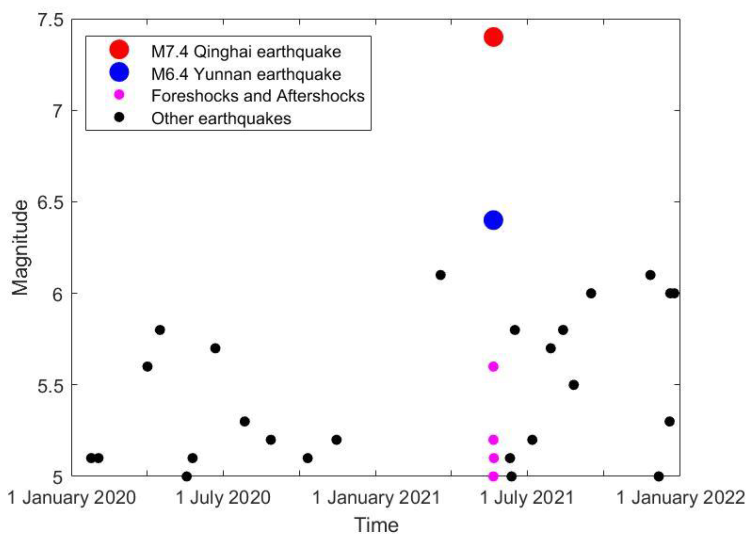
2.1. Data and Study Area
2.2. Anomalies Detection
2.2.1. LSTM Model
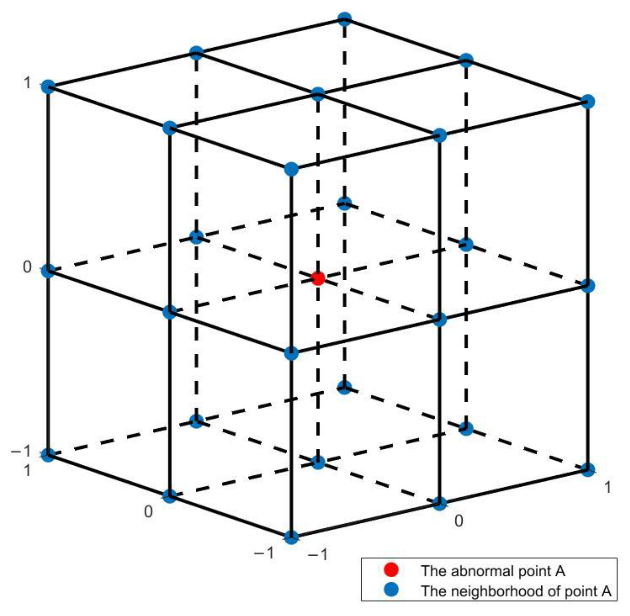
2.2.2. Relative Power Spectrum
2.3. Statistical Method
3. Results and Discussion
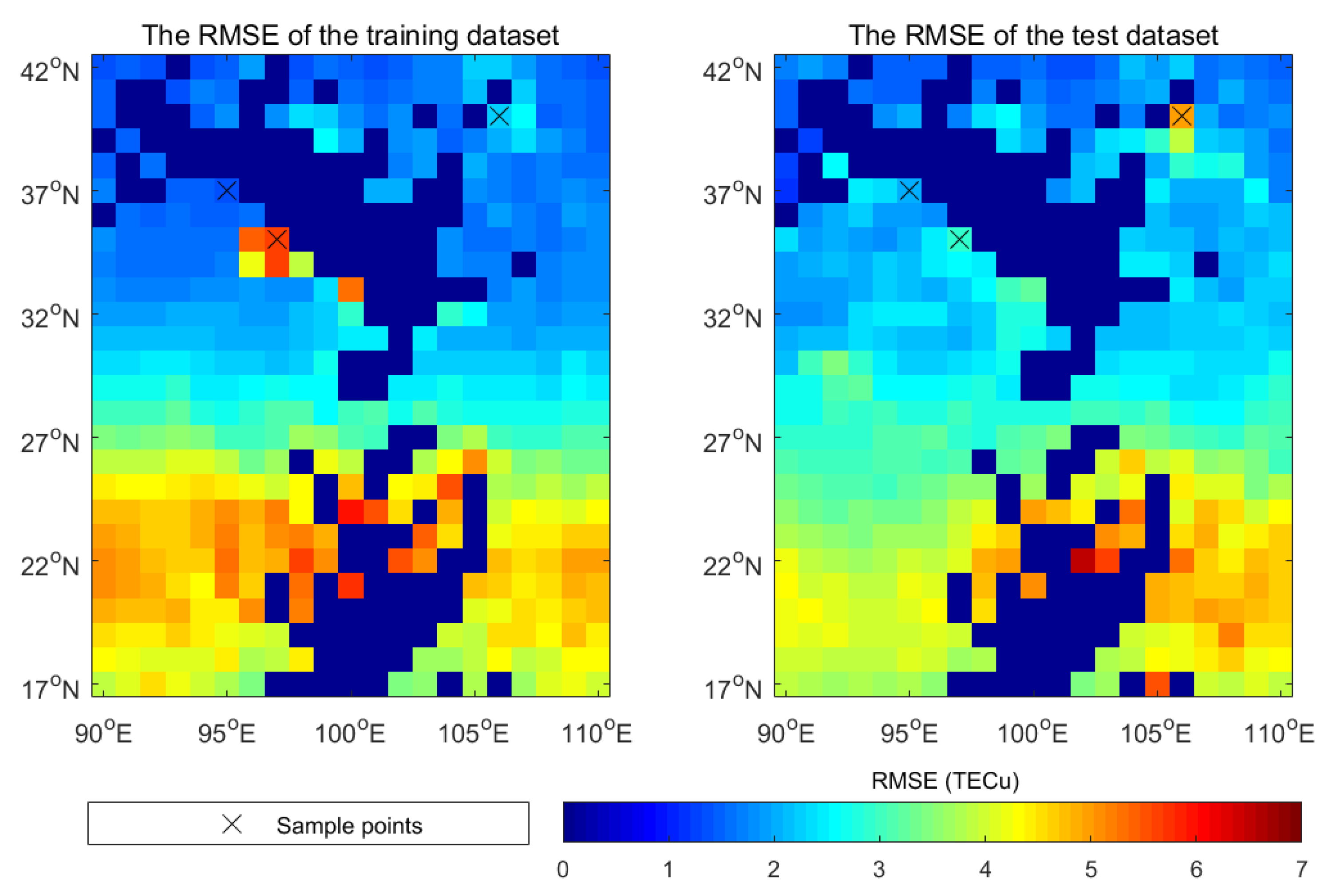
3.1. LSTM Model Performance
3.2. Statistic Result
3.3. Cases Study
4. Conclusions
Author Contributions
Funding
Data Availability Statement
Conflicts of Interest
References
- Tramutoli, V.; Aliano, C.; Corrado, R.; Filizzola, C.; Genzano, N.; Lisi, M.; Martinelli, G.; Pergola, N. On the possible origin of thermal infrared radiation (TIR) anomalies in earthquake-prone areas observed using robust satellite techniques (RST). Chem. Geol. 2013, 339, 157–168. [Google Scholar] [CrossRef]
- Jiao, Z.-H.; Zhao, J.; Shan, X. Pre-seismic anomalies from optical satellite observations: A review. Nat. Hazards Earth Syst. Sci. 2018, 18, 1013–1036. [Google Scholar] [CrossRef]
- Freund, F.; Ouillon, G.; Scoville, J.; Sornette, D. Earthquake precursors in the light of peroxy defects theory: Critical review of systematic observations. Eur. Phys. J. Spec. Top. 2021, 230, 7–46. [Google Scholar] [CrossRef]
- Pulinets, S.; Ouzounov, D. Lithosphere Atmosphere ionosphere coupling (LAIC) model—An unified concept for earthquake precursors validation. J. Asian Earth Sci. 2011, 41, 371–382. [Google Scholar] [CrossRef]
- Liperovsky, V.A.; Pokhotelov, O.A.; Meister, C.V.; Liperovskaya, E.V. Physical models of coupling in the lithosphere-atmosphere-ionosphere system before earthquakes. Geomagn. Aeron. 2008, 48, 795–806. [Google Scholar] [CrossRef]
- Qu, C.-Y.; Ma, J.; Shan, X.-J. Counterevidence for an Earthquake Precursor of Satellite Thermal Infrared Anomalies. Chin. J. Geophys. 2006, 49, 426–431. [Google Scholar] [CrossRef]
- Chiodini, G.; Cardellini, C.; Di Luccio, F.; Selva, J.; Frondini, F.; Caliro, S.; Rosiello, A.; Beddini, G.; Ventura, G. Correlation between tectonic CO2 Earth degassing and seismicity is revealed by a 10-year record in the Apennines, Italy. Sci. Adv. 2020, 6, 35. [Google Scholar] [CrossRef]
- Spogli, L.; Alfonsi, L.; De Franceschi, G.; Romano, V.; Aquino, M.H.O.; Dodson, A. Climatology of GPS ionospheric scintillations over high and mid-latitude European regions. Ann. Geophys. 2009, 27, 3429–3437. [Google Scholar] [CrossRef]
- Jakowski, N.; Mayer, C.; Hoque, M.M.; Wilken, V. Total electron content models and their use in ionosphere monitoring. Radio Sci. 2011, 46, RS0D18. [Google Scholar] [CrossRef]
- Kuo, C.L.; Lee, L.C.; Huba, J.D. An improved coupling model for the lithosphere-atmosphere-ionosphere system. J. Geophys. Res. Space Phys. 2014, 119, 3189–3205. [Google Scholar] [CrossRef]
- Akhoondzadeh, M.; Parrot, M.; Saradjian, M.R. Electron and ion density variations before strong earthquakes (M > 6.0) using DEMETER and GPS data. Nat. Hazards Earth Syst. Sci. 2010, 10, 7–18. [Google Scholar] [CrossRef]
- Saradjian, M.R.; Akhoondzadeh, M. Prediction of the date, magnitude and affected area of impending strong earthquakes using integration of multi precursors earthquake parameters. Nat. Hazards Earth Syst. Sci. 2011, 11, 1109–1119. [Google Scholar] [CrossRef]
- Liu, C.-Y.; Liu, J.-Y.; Chen, Y.-I.; Qin, F.; Chen, W.-S.; Xia, Y.-Q.; Bai, Z.Q. Statistical analyses on the ionospheric total electron content related to M ≥ 6.0 earthquakes in China during 1998–2015. Terr. Atmos. Ocean. Sci. 2018, 29, 485–498. [Google Scholar] [CrossRef]
- Akhoondzadeh, M.; De Santis, A.; Marchetti, D.; Shen, X. Swarm-TEC satellite measurements as a potential earthquake precursor together with other Swarm and CSES data: The case of Mw 7.6 2019 Papua New Guinea seismic event. Front. Earth Sci. 2022, 10, 820189. [Google Scholar] [CrossRef]
- Akhoondzadeh, M.; Saradjian, M.R. TEC variations analysis concerning Haiti (January 12, 2010) and Samoa (September 29, 2009) earthquakes. Adv. Space Res. 2011, 47, 94–104. [Google Scholar] [CrossRef]
- Akhoondzadeh, M. Support vector machines for TEC seismo-ionospheric anomalies detection. Ann. Geophys. 2013, 31, 173–186. [Google Scholar] [CrossRef]
- Akhoondzadeh, M. An Adaptive Network-based Fuzzy Inference System for the detection of thermal and TEC anomalies around the time of the Varzeghan, Iran, (Mw = 6.4) earthquake of 11 August 2012. Adv. Space Res. 2013, 52, 837–852. [Google Scholar] [CrossRef]
- Akhoondzadeh, M. A MLP neural network as an investigator of TEC time series to detect seismo-ionospheric anomalies. Adv. Space Res. 2013, 51, 2048–2057. [Google Scholar] [CrossRef]
- Akhoondzadeh, M. Investigation of GPS-TEC measurements using ANN method indicating seismo-ionospheric anomalies around the time of the Chile (Mw = 8.2) earthquake of April 01 2014. Adv. Space Res. 2014, 54, 1768–1772. [Google Scholar] [CrossRef]
- Akhoondzadeh, M. Genetic algorithm for TEC seismo-ionospheric anomalies detection around the time of the Solomon (Mw= 8.0) earthquake of 06 February 2013. Adv. Space Res. 2013, 52, 581–590. [Google Scholar] [CrossRef]
- Xiong, P.; Zhai, D.; Long, C.; Zhou, H.; Zhang, X.; Shen, X. Long short-term memory neural network for ionospheric total electron content forecasting over China. Space Weather 2021, 19, e2020SW002706. [Google Scholar] [CrossRef]
- Saqib, M.; Şentürk, E.; Sahu, S.A.; Adil, M.A. Comparisons of autoregressive integrated moving average (ARIMA) and long short term memory (LSTM) network models for ionospheric anomalies detection: A study on Haiti (Mw = 7.0) earthquake. Acta Geod. Geophys. 2022, 57, 195–213. [Google Scholar] [CrossRef]
- Akhoondzadeh, M.; De Santis, A.; Marchetti, D.; Wang, T. Developing a Deep Learning-Based Detector of Magnetic, Ne, Te and TEC Anomalies from Swarm Satellites: The Case of Mw 7.1 2021 Japan Earthquake. Remote Sens. 2022, 14, 1582. [Google Scholar] [CrossRef]
- Zhang, Y.S.; Guo, X.; Wei, C.X.; Shen, W.R.; Hui, S.X. Characteristics of seismic thermal radiation of the Japan Ms9. 0 and Myanmar Ms7. 2 earthquake. Chin. J. Geophys. 2011, 54, 670–676. [Google Scholar] [CrossRef]
- Wei, C.; Zhang, Y.; Guo, X.; Hui, S.; Qin, M.; Zhang, Y. Thermal infrared anomalies of several strong earthquakes. Sci. World J. 2013, 2013, 208407. [Google Scholar] [CrossRef] [PubMed]
- Zhang, X.; Zhang, Y.S.; Tian, X.F.; Zhang, Q.L.; Tian, J. Tracking of Thermal Infrared Anomaly before One Strong Earthquake-In the Case of Ms6.2 Earthquake in Zadoi, Qinghai on October 17th, 2016. J. Phys. Conf. Ser. 2017, 910, 012048. [Google Scholar] [CrossRef]
- Zhang, Y.; Meng, Q.Y. A statistical analysis of TIR anomalies extracted by RSTs in relation to an earthquake in the Sichuan area using MODIS LST data. Nat. Hazards Earth Syst. Sci. 2019, 19, 535–549. [Google Scholar] [CrossRef]
- Zechar, J.D.; Jordan, T.H. Testing alarm-based earthquake predictions. Geophys. J. Int. 2008, 72, 715–724. [Google Scholar] [CrossRef]
- Ikuta, R.; Oba, R. How credible are earthquake predictions based on TEC variations? J. Geophys. Res. Space Phys. 2022, 127, e2021JA030151. [Google Scholar] [CrossRef]
- Parsons, T. On the use of receiver operating characteristic tests for evaluating spatial earthquake forecasts. Geophys. Res. Lett. 2020, 47, c2020GL088570. [Google Scholar] [CrossRef]
- Klimenko, M.V.; Klimenko, V.V.; Zakharenkova, I.E.; Pulinets, S.A.; Zhao, B.; Tsidilina, M.N. Formation mechanism of great positive TEC disturbances prior to Wenchuan earthquake on May 12, 2008. Adv. Space Res. 2011, 48, 488–499. [Google Scholar] [CrossRef]
- Akhoondzadeh, M. Anomalous TEC variations associated with the powerful Tohoku earthquake of 11 March 2011. Nat. Hazards Earth Syst. Sci. 2012, 12, 1453–1462. [Google Scholar] [CrossRef]
- Tariq, M.A.; Shah, M.; Hernández-Pajares, M.; Iqbal, T. Pre-earthquake ionospheric anomalies before three major earthquakes by GPS-TEC and GIM-TEC data during 2015–2017. Adv. Space Res. 2019, 63, 2088–2099. [Google Scholar] [CrossRef]
- Zhu, F.; Wu, Y.; Zhou, Y.; Lin, J. A statistical investigation of pre-earthquake ionospheric TEC anomalies. Geod. Geodyn. 2011, 2, 61–65. [Google Scholar]
- Kon, S.; Nishihashi, M.; Hattori, K. Ionospheric anomalies possibly associated with M P6.0 earthquakes in the Japan area during 1998–2010: Case studies and statistical study. J. Asian Earth Sci. 2011, 41, 410–420. [Google Scholar] [CrossRef]
- Rideout, W.C.; Coster, A. Automated GPS processing for global total electron content data. GPS Solut. 2006, 10, 219–228. [Google Scholar] [CrossRef]
- Jing, F.; Zhang, L.; Singh, R.P. Pronounced Changes in Thermal Signals Associated with the Madoi (China) M 7.3 Earthquake from Passive Microwave and Infrared Satellite Data. Remote Sens. 2022, 14, 2539. [Google Scholar] [CrossRef]
- Chen, W.K.; Wang, D.; Zhang, C.; Yao, Q.; Si, H.J. Estimating Seismic Intensity Maps of the 2021 Mw 7.3 Madoi, Qinghai and Mw 6.1 Yangbi, Yunnan, China Earthquakes. J. Earth Sci. 2022, 33, 839–846. [Google Scholar] [CrossRef]
- Yu, Y.; Si, X.; Hu, C.; Zhang, J. A Review of Recurrent Neural Networks: LSTM Cells and Network Architectures. Neural Comput. 2019, 31, 1235–1270. [Google Scholar] [CrossRef]
- Tang, J.; Li, Y.; Ding, M.; Liu, H.; Yang, D.; Wu, X. An Ionospheric TEC Forecasting Model Based on a CNN-LSTM-Attention Mechanism Neural Network. Remote Sens. 2022, 14, 2433. [Google Scholar] [CrossRef]
- Willmott, C.J.; Matsuura, K. Advantages of the mean absolute error (MAE) over the root mean square error (RMSE) in assessing average model performance. Clim. Res. 2005, 30, 79–82. [Google Scholar] [CrossRef]
- Wei, C.; Lu, X.; Zhang, Y.; Guo, Y.; Wang, Y. A time-frequency analysis of the thermal radiation background anomalies caused by large earthquakes: A case study of the Wenchuan 8.0 earthquake. Adv. Space Res. 2020, 65, 435–445. [Google Scholar] [CrossRef]
- Shcherbakov, R.; Turcotte, D.L.; Rundle, J.B.; Tiampo, K.F.; Holliday, J.R. Forecasting the Locations of Future Large Earthquakes: An Analysis and Verification. Pure Appl. Geophys. 2010, 167, 743–749. [Google Scholar] [CrossRef][Green Version]
- Li, S.H.; Galas, R.; Ewert, D.; Peng, J.H. An Empirical Model for the Ionospheric Global Electron Content Storm-Time Response. Acta Geophys. 2016, 64, 253–269. [Google Scholar] [CrossRef]
- Loewe, C.A.; Prölss, G.W. Classification and mean behavior of magnetic storms. J. Geophys. Res. Space Phys. 1997, 102, 14209–14213. [Google Scholar] [CrossRef]
- Ouzounov, D.; Pulinets, S.; Davidenko, D.; Rozhnoi, A.; Solovieva, M.; Fedun, V.; Dwivedi, B.N.; Rybin, A.; Kafatos, M.; Taylor, P. Transient Effects in Atmosphere and Ionosphere Preceding the 2015 M7.8 and M7.3 Gorkha–Nepal Earthquakes. Front. Earth Sci. 2021, 9, 757358. [Google Scholar] [CrossRef]


| Earthquake Time (UTC) | Magnitude | Latitude (°E) | Longitude (°N) | Depth (km) | Type |
|---|---|---|---|---|---|
| 24 January 2020 22:56:05 | 5.1 | 31.98 | 95.09 | 10 | Mainshock |
| 2 February 2020 16:05:41 | 5.1 | 30.74 | 104.46 | 21 | Mainshock |
| 1 April 2020 12:23:27 | 5.6 | 33.04 | 98.92 | 10 | Mainshock |
| 16 April 2020 11:45:25 | 5.8 | 22.72 | 94.00 | 10 | Mainshock |
| 18 May 2020 13:47:59 | 5.0 | 27.18 | 103.16 | 8 | Mainshock |
| 25 May 2020 14:42:16 | 5.1 | 24.35 | 93.85 | 60 | Mainshock |
| 21 June 2020 22:40:53 | 5.7 | 23.15 | 93.25 | 30 | Mainshock |
| 27 July 2020 05:14:48 | 5.3 | 20.90 | 104.70 | 10 | Mainshock |
| 27 August 2020 12:07:15 | 5.2 | 23.00 | 93.20 | 10 | Mainshock |
| 10 October 2020 17:38:00 | 5.1 | 24.70 | 93.65 | 40 | Mainshock |
| 14 November 2020 08:50:26 | 5.2 | 23.55 | 94.65 | 100 | Mainshock |
| 19 March 2021 06:11:26 | 6.1 | 31.94 | 92.74 | 10 | Mainshock |
| 21 May 2021 13:21:25 | 5.6 | 25.63 | 99.92 | 10 | Foreshock |
| 21 May 2021 13:48:34 | 6.4 | 25.67 | 99.87 | 8 | Mainshock |
| 21 May 2021 13:55:28 | 5.0 | 25.67 | 99.89 | 8 | Aftershock |
| 21 May 2021 14:31:10 | 5.2 | 25.59 | 99.97 | 8 | Aftershock |
| 21 May 2021 18:04:11 | 7.4 | 34.59 | 98.34 | 17 | Mainshock |
| 22 May 2021 02:29:34 | 5.1 | 34.85 | 97.50 | 10 | Aftershock |
| 10 June 2021 11:46:07 | 5.1 | 24.34 | 101.91 | 8 | Mainshock |
| 12 June 2021 10:00:46 | 5.0 | 24.96 | 97.89 | 16 | Mainshock |
| 16 June 2021 16:48:58 | 5.8 | 38.14 | 93.81 | 10 | Mainshock |
| 7 July 2021 14:43:48 | 5.2 | 19.65 | 101.20 | 10 | Mainshock |
| 29 July 2021 16:39:27 | 5.7 | 22.70 | 96.04 | 20 | Mainshock |
| 13 August 2021 12:21:35 | 5.8 | 34.58 | 97.54 | 8 | Mainshock |
| 26 August 2021 07:38:18 | 5.5 | 38.88 | 95.50 | 15 | Mainshock |
| 16 September 2021 04:33:31 | 6.0 | 29.20 | 105.34 | 10 | Mainshock |
| 26 November 2021 07:45:42 | 6.1 | 22.70 | 93.40 | 50 | Mainshock |
| 6 December 2021 08:25:38 | 5.0 | 23.23 | 96.17 | 10 | Mainshock |
| 19 December 2021 07:54:28 | 5.3 | 38.95 | 92.73 | 10 | Mainshock |
| 20 December 2021 05:06:14 | 6.0 | 19.60 | 101.40 | 10 | Mainshock |
| 24 December 2021 21:43:21 | 6.0 | 22.33 | 101.69 | 15 | Mainshock |
| Position | 106°E, 40°N | 97°E, 35°N | 95°E, 37°N |
|---|---|---|---|
| Train RMSE | 2.2807 | 5.6363 | 1.3819 |
| Test RMSE | 5.0072 | 2.9243 | 2.0781 |
| Parameters | Intensity Threshold Ti | Duration Threshold (Td, Days) | Area Threshold (Ta, Pixels) | Predicted Time Window (W, Days) | Predicted Radius (R, km) |
|---|---|---|---|---|---|
| Value | 5, 10, 15, 20 | 1, 2, 3, 4, 5, 6, 7 | 1, 2, 3, 4, 5 | 14, 28, 42, 56 | 100, 200, 300, 400, 500 |
| Group Number | Tv | Td (days) | Ta (pixels) | W (days) | R (km) | CR | ν | G |
|---|---|---|---|---|---|---|---|---|
| 1 | 5 | 3 | 2 | 28 | 300 | 0.10 | 0.40 | 1.91 |
| 2 | 5 | 2 | 2 | 28 | 300 | 0.10 | 0.40 | 1.68 |
| 3 | 15 | 1 | 1 | 14 | 400 | 0.08 | 0.46 | 1.59 |
| 4 | 5 | 6 | 2 | 42 | 400 | 0.22 | 0.50 | 1.58 |
| 5 | 5 | 6 | 2 | 56 | 400 | 0.27 | 0.42 | 1.58 |
| 6 | 5 | 6 | 1 | 56 | 300 | 0.19 | 0.50 | 1.58 |
| 7 | 15 | 1 | 1 | 14 | 500 | 0.12 | 0.31 | 1.57 |
| 8 | 5 | 3 | 2 | 42 | 300 | 0.14 | 0.38 | 1.56 |
| 9 | 5 | 1 | 2 | 28 | 300 | 0.08 | 0.40 | 1.56 |
| 10 | 15 | 1 | 1 | 28 | 300 | 0.10 | 0.44 | 1.55 |
Publisher’s Note: MDPI stays neutral with regard to jurisdictional claims in published maps and institutional affiliations. |
© 2022 by the authors. Licensee MDPI, Basel, Switzerland. This article is an open access article distributed under the terms and conditions of the Creative Commons Attribution (CC BY) license (https://creativecommons.org/licenses/by/4.0/).
Share and Cite
Yue, Y.; Koivula, H.; Bilker-Koivula, M.; Chen, Y.; Chen, F.; Chen, G. TEC Anomalies Detection for Qinghai and Yunnan Earthquakes on 21 May 2021. Remote Sens. 2022, 14, 4152. https://doi.org/10.3390/rs14174152
Yue Y, Koivula H, Bilker-Koivula M, Chen Y, Chen F, Chen G. TEC Anomalies Detection for Qinghai and Yunnan Earthquakes on 21 May 2021. Remote Sensing. 2022; 14(17):4152. https://doi.org/10.3390/rs14174152
Chicago/Turabian StyleYue, Yingbo, Hannu Koivula, Mirjam Bilker-Koivula, Yuwei Chen, Fuchun Chen, and Guilin Chen. 2022. "TEC Anomalies Detection for Qinghai and Yunnan Earthquakes on 21 May 2021" Remote Sensing 14, no. 17: 4152. https://doi.org/10.3390/rs14174152
APA StyleYue, Y., Koivula, H., Bilker-Koivula, M., Chen, Y., Chen, F., & Chen, G. (2022). TEC Anomalies Detection for Qinghai and Yunnan Earthquakes on 21 May 2021. Remote Sensing, 14(17), 4152. https://doi.org/10.3390/rs14174152