Article

Road-Side Individual Tree Segmentation from Urban MLS Point Clouds Using Metric Learning

1
Blueprint Idea Technology Development Company Limited, Beijing 100020, China
2
Beijing Career International Company Limited, Beijing 100020, China
3
Key Laboratory of Virtual Geographic Environment, Ministry of Education, Nanjing Normal University, Nanjing 210093, China
4
College of Computer Science and Engineering, Northwest Normal University, Lanzhou 730070, China
5
State Key Laboratory of Information Engineering in Surveying Mapping and Remote Sensing, Wuhan University, Wuhan 430079, China
*
Author to whom correspondence should be addressed.
These authors contribute equally to this work.
Remote Sens. 2023, 15(8), 1992; https://doi.org/10.3390/rs15081992
Submission received: 27 February 2023 / Revised: 3 April 2023 / Accepted: 7 April 2023 / Published: 10 April 2023

Abstract

:
As one of the most important components of urban space, an outdated inventory of road-side trees may misguide managers in the assessment and upgrade of urban environments, potentially affecting urban road quality. Therefore, automatic and accurate instance segmentation of road-side trees from urban point clouds is an important task in urban ecology research. However, previous works show under- or over-segmentation effects for road-side trees due to overlapping, irregular shapes and incompleteness. In this paper, a deep learning framework that combines semantic and instance segmentation is proposed to extract single road-side trees from vehicle-mounted mobile laser scanning (MLS) point clouds. In the semantic segmentation stage, the ground points are filtered to reduce the processing time. Subsequently, a graph-based semantic segmentation network is developed to segment road-side tree points from the raw MLS point clouds. For the individual tree segmentation stage, a novel joint instance and semantic segmentation network is adopted to detect instance-level roadside trees. Two complex Chinese urban point cloud scenes are used to evaluate the individual urban tree segmentation performance of the proposed method. The proposed method accurately extract approximately 90% of the road-side trees and achieve better segmentation results than existing published methods in both two urban MLS point clouds. Living Vegetation Volume (LVV) calculation can benefit from individual tree segmentation. The proposed method provides a promising solution for ecological construction based on the LVV calculation of urban roads.

1. Introduction

Statistics show that more than half of the world’s population lives in cities. By the middle of the 21st century, this proportion is expected to rise to 70% [1]. The more serious truth is that cities that account for less than 3% of the earth’s surface consume more than 75% of natural resources. Vegetation has the function of eliminating harmful pollutants, reducing noise, regulating temperature, protecting water sources, and providing various renewable energy sources [2,3,4]. If vegetation solutions can be reasonably incorporated into urban, methods similar to urban tree inventory are bound to overcome a series of existing challenges. To obtain comprehensive and accurate urban tree information, various emerging technologies have gradually replaced traditional manual measurement methods, such as photogrammetry and remote sensing [5,6,7]. In particular, the rapidly developing LiDAR technology offers a promising method for capturing urban point clouds, demonstrating its brilliance in large-scale mapping scenes [8].
LiDAR is different from images limited by low resolution, weather sensitivity, and poor penetration, and its advantages include high precision, high resolution, and flexibility [9,10,11]. Most importantly, they can reflect the detailed three-dimensional spatial distribution of trees at the individual level, which provides a new perspective for tree inventory. As we all know, urban tree inventory requires not only accurate spatial information but also individual tree parameters [12]. For management purposes, the timely update of spatial information such as the distribution of trees and the location of an individual tree helps maintain reliable monitoring of urban trees. The separation of woody parts and leaves provides a basis for the calculation of individual tree parameters such as species classification, leaf area index (LAI) estimation, crown volume estimation, and diameter at breast height (DBH) estimation [13,14,15,16]. Therefore, instance segmentation of urban trees and the separation of wood and leaf points for individual trees are indispensable and important components [17]. However, the acquired point clouds are all unorganized and huge, which makes these two tasks technically challenging.
The above-mentioned research and results inspired us to use a deep learning network to extract a single tree from the point cloud and further distinguish the wood–leaf points. Therefore, in this article, we propose a new type of network applied to complex cities to give full play to the potential and advantages of the combination of semantic segmentation and instance segmentation [18] and contribute at least the following double aspects:
  • A novel individual tree segmentation framework that combines semantic and instance segmentation network is designed to separate instance-level road-side trees from point clouds.
  • Extensive experiments on two mobile laser scanning (MLS) and one airborne laser scanning (ALS) point clouds have been carried out to demonstrate the effectiveness and generalization of the proposed tree segmentation method for urban scenes.

2. Related Work

First, we briefly survey point cloud semantic and instance segmentation, which inspires our study. Next, we present a review of recent progress regarding individual tree segmentation from point clouds.

2.1. Point Cloud Semantic Segmentation

Point cloud semantic segmentation is a practical solution to interpret information of the 3D scene from point clouds, which aims to annotate each point in a given point cloud with a label of semantic meaning [19]. Previous works solve the problem of point cloud semantic segmentation by applying supervised classification models in accordance with handcrafted features [20,21,22]. The performances of these methods usually depend on two very important factors: distinctive hand-crafted features (i.e., geometry features, waveform-based features, topology features, and contextual features from spatial distributions) and discriminative classifiers (i.e., support vector machines, random forest, Hough forest, and Markov random fields) [23,24,25,26]. However, the calculation of effective handcrafted features requires a large number of prior knowledge, which has limited ability to learn good features of the scanned objects [27].
To mitigate burdens in feature design, deep learning for point cloud semantic segmentation has drawn increasingly considerable attention because it provides an end-to-end solution [28,29,30]. Therefore, deep-learning-based methods have become the dominant technologies in the point cloud semantic segmentation task. As discussed in [31], there are four main paradigms of neural networks for point clouds semantic segmentation, such as projection-based methods [32,33,34] that usually project a 3D point cloud into 2D images, discretization-based methods [35,36,37] that usually transform a point cloud into a discrete representation, point-based networks [38,39,40] that directly work on the irregular point cloud, and graph-based methods [41,42,43] that construct an adjacency graph to model the neighboring relations among the points. On the whole, the great success in point cloud semantic segmentation has made it easier to divide raw point clouds into several certain types of object points, which is helpful for extracting tree points from raw point clouds [44].

2.2. Point Cloud Instance Segmentation

The goal of point cloud instance segmentation is to separate a given point cloud into some instance-level objects. The existing methods can be roughly divided into two groups: proposal-based methods [45,46,47,48,49] and proposal-free methods [50,51,52,53,54]. The proposal-based methods are usually considered as the top-down strategies, which converts instance segmentation into two sub-problems, the region proposal generation and the instance object prediction. The proposal-based methods can simply segment the object within each proposal, but they usually require multi-stage training and pruning redundant proposals, resulting in more computer memory. By contrast, the proposal-free methods have a low computational cost. The proposal-free methods depend on a bottom-up pipeline that produces per-point predictions (such as point-wise semantic labels and center offset vectors) then groups points of the same labels with small geometric distances into instances [55]. With the help of semantic segmentation, the proposal-free methods can generate high-quality proposals. However, they have two main disadvantages: (1) low overlap between predicted and the ground-truth instance, (2) false-positive instances from wrong semantic segmentation results.
Although most existing point cloud instance segmentation methods have achieved significant progress in indoor scene point clouds, the performance of the outdoor urban MLS point clouds is often low since objects are locally ambiguous in many cases. In addition, the boundaries between adjacent road-side trees are usually blurred, making instance segmentation methods hard to be generalized to the individual tree separation task. However, these instance segmentation methods can also provide inspiration for the instance-level tree segmentation from urban MLS point clouds.

2.3. Individual Tree Segmentation

In the past decade, various clustering methods to varying degrees have been applied to obtain better segmentation results. Chen et al. [56] compared four different single tree extraction methods: Euclidean distance classification, region growing, normalized cutting, and supervoxel segmentation, and found that the application of the N-cut method after Euclidean distance clustering can obtain better segmentation results. Furthermore, various automated methods for extracting individual trees from point clouds have been proposed, which can be roughly divided into geometry-based unsupervised methods [57,58,59] and a supervision method based on semantic annotation [60,61,62]. These methods can process some trees with simple structures through tedious and labor-intensive parameter tuning, but they still lack generalization ability on the instance-level separation of trees with different shapes and canopy structures.
Benefiting from the advances in neural network architectures and their great potential in improving the generality and accuracy of point cloud segmentation, there are several works that successfully achieved the individual tree segmentation from the point cloud using deep learning methods [63]. Following an idea similar to the instance segmentation, Wang et al. [64] propose a point-wise semantic learning network to acquire both local and global information. By avoiding the information loss and reducing useless convolutional computations, it is an effective approach for individual tree segmentation from ALS point clouds. To automatically extract urban trees from large-scale point clouds, PointNLM [65] incorporates the supervoxel-based and point-wise methods for capturing the long-range relationship. Simultaneously, a fusion layer of neighborhood max-pooling method is developed to concatenate the multi-level features for separating the road-side trees. For tree detection, Luo et al. [66] design a top-down slice module, which can effectively mine the vertical structure information in a top-down way. To detect trees more accurately, Luo et al. [66] also add a multi-branch network for providing discriminative information by fusing multichannel features. To extract individual urban trees from MLS point clouds, Luo et al. [67] develop a novel top-down framework, called DAE_Net, based on semantic and instance segmentation network. After that, the boundaries of instance-level trees are enhanced by predicting the direction vector for isolated tree clusters.

3. Methodology

As shown in Figure 1, the proposed framework consists of two stages: road-side tree extraction by semantic segmentation and individual tree separation by instance segmentation.

3.1. Tree Point Extraction

Generally, an MLS system has a relatively direct scanning angle of view of the ground. Therefore, the collected 3D points contain massive ground points, which undoubtedly increase algorithm complexity. A fast and effective preprocessing method is adopted to separate ground points from original point clouds to reduce the data search range of point cloud processing. In addition, the ground points are projected and resampled to obtain the digital elevation model of corresponding region, which is of great significance for the subsequent calculation of tree height features.
There are often inevitable ups and downs on the ground in an entire urban scene [68]. The filtering effect of ground points is not ideal considering the influence of the accuracy of the initial triangulated irregular network (TIN). An improved progressive TIN densification filtering method is introduced to remove ground points. The undetermined seed points were first selected by the extended local minimum for grids containing points. Then, the elevations of the grids without points are interpolated using the nearest-neighbor method. The final seed points are determined according to the judgment of the elevation difference (ED) in the local neighborhood of thin-plate spline interpolation with the threshold. Finally, the initial TIN is constructed and iteratively encrypted to extract the ground points [69].
The complexity of an urban scene is the main obstacle to semantically extracting tree points, which usually contain many categories of objects as well as overlapping or closely positioned objects [20]. This study proposes a graph convolution network (GCN) that integrates a lightweight representation learning module and a deep context-aware sequential module with embedded residual learning to classify urban scenes into tree and non-tree point clouds.
Unstructured point clouds are first divided into geometrically homogeneous parts to ameliorate non-uniform distribution and reduce computational complexity. The geometric grouping algorithm is adopted from [41] which directly consumes original LiDAR point clouds generating clusters with approximately equal resolution. A sparse auto-encoder is employed to compress and encode high-dimensional information as the embedding to represent the geometric attributes of every patch. Moreover, the spatial position of geometric clusters is considered to be concatenated into the final descriptor to increase spatial relationships. To promote the formation of associated areas from geometric patches generated from the non-ground points, an adjacency graph G = V ,   E is constructed to model neighboring relationships among the patches. The center of precomputed patches acts as the nodes V = v i in the G , and edges E = e i j are established between each pair of adjacent patches to allow the network to be relatively robust in handling varying point densities. Specifically, variable adjacency is adopted instead of a fixed-size neighborhood.
There is no spatial transformer network (STN) chosen to match the groups because the geometric groups are computed based on normalization. Specific feature extraction for geometric groupings is performed as follows. First, node feature F n is obtained using a multilayer perceptron (MLP). Then, k neighboring points of the node is found using the k-nearest neighbor (KNN) algorithm, and the neighborhood coordinates X c k of each node are obtained. The spatial position information of the neighboring point feature set F c k obtained through the neighborhood point subscript attributes is further encoded. This structure encodes the 3D geometric information of nodes (the coordinates) and the connection with corresponding neighbors (the Euclidean distance X c X c k ). An MLP with a 3-layer fully connected structure adjusted the weights of the four spatial position information and extracted geometric features F G . The convolution operation on the node feature and the neighboring point feature obtained the semantic feature F S so that the extraction of the local and context information is more detailed. Finally, the geometric features encoded by the geometric coordinate, node association information, and neighboring point features are weighted and summed to form the neighborhood feature set F C S G . Edge features are determined by the filter-generating network that dynamically produces weights for filtering edge-specific information through element-wise multiplication [70].
The last step of semantic segmentation involves group-wise labeling by employing a GCN to classify the Voronoi adjacency graph. A residual net architecture is used for semantic segmentation to accelerate convergence and prediction [71]. The input is a graph with a varying number of edges and nodes, with some regular neural networks unable to cope with such structures. Therefore, long short-term memory [72] is chosen with an input gate while incorporating the residual connections. This technique can handle graphs with varying sizes while avoiding the vanishing gradient problem.
Only the tree points are used for further individual urban tree segmentation from the various classes of obtained point clouds.

3.2. Individual Tree Segmentation

After the object tree is extracted, we further carry out the individual tree segmentation task. Traditionally, there are two commonly used individual tree segmentation methods: the CHM-based segmentation methods [6] and the cluster-based graph cut methods [73]. CHM-based segmentation method can quickly segment tree point clouds, but the CHM transformation can result in the loss of most crucial geometric and spatial context attributes. By contrast, the cluster-based graph cut method can preserve 3D spatial context information. However, too many parameters will result in high computational costs. In addition, the regular clustering strategies are completely insensitive to the boundary, which makes fine segmentation in the complex tree scene very difficult. Recently, point cloud processing has achieved significant progress with the development of deep learning techniques [64,65,66,67], which makes it possible to extract individual trees from point clouds. To effectively extract individual trees from urban MLS point clouds, we propose a novel segmentation network that combines the semantic information (spatial context information) of the tree category and the instance information of each tree. In this section, we elaborate on the proposed individual tree segmentation method in three parts, namely density-based point convolution, associatively segmenting instances and semantics in tree point clouds, and loss function based on metric learning. The overview of the proposed individual tree segmentation method is shown in Figure 2.

3.2.1. Density-Based Point Convolution (DPC)

In general, 2D convolution kernel cannot be applied to scattered and disordered point clouds. PointNet-series networks are the earliest architectures that extract features directly from points. PointNet uses the Multi-layer Perceptron (MLP) with shared weight to process the point cloud by weighted summation and solves the disorder of the point cloud through the maximum pooling operation. However, maximum pool (MP) operation is easy to cause local information loss of point cloud. To improve the ability of point information extraction, the weight of the convolution operator is treated as a continuous function composed of local context information relative to the reference point. For the functions f(x) and g(x) of d-dimensional vector x, the definition formula of convolution is shown as follows:
f × g x = τ d f τ g x + τ d τ ,
It can be interpreted as a 2D discrete function in the image, which is usually represented by a grid matrix. In the convolution neural network, the convolution kernel acts on a fixed size local area for weighted sum operation. The relative position between pixels in the image is fixed; therefore, the filter can be discretized into weighted summation with corresponding positions in each local region.
Unlike images, point cloud data is scattered and disordered. Each point in the point cloud is an arbitrary continuous value, rather than distributed on a fixed grid. Traditional convolutional filters used on images cannot be directly utilized on point clouds. To make full use of convolutional operations on point clouds, a permutation-invariant convolutional filter, called PointCONV [74], is used to define the 3D convolutions for continuous functions by
Conv W ,   F x y z = δ x , δ y , δ z G W δ x , δ y , δ z F x + δ x , y + δ y , z + δ z d δ x δ y δ z ,
where W and F are two functions, F x + δ x , y + δ y , z + δ z indicates the contextual feature of a point p i (i = 1, 2, …, n) in the local neighborhood E, where (x, y, z) is the center position of this local region. There is a difference in the density between the canopy points and the trunk points in the tree point cloud. Therefore, density information is extracted to construct density-based point convolution, as follows:
DensityConv S , W ,   F x y z = δ x , δ y , δ z G S δ x , δ y , δ z W δ x , δ y , δ z F x + δ x , y + δ y , z + δ z ,
where S δ x , δ y , δ z represents the inverse density given the local neighborhood point δ x , δ y , δ z . Because the down-sampled point clouds are non-uniformly distributed, density-based weighting is very important. The weight function W δ x , δ y , δ z is constructed through MLP. The inverse density function S δ x , δ y , δ z is constructed by kernel density estimation, and then nonlinear transformation is realized by using MLP. The density point convolution aiming at the arrangement invariance is constructed through the MLP with shared weight. The density parameters of each point in the fixed neighborhood are calculated based on the kernel density estimation function, and the density parameters are transformed nonlinearly through MLP. The appropriate density function is learned adaptively, and the final inverse density scale is calculated.
Figure 3 shows the operation of density-based point convolution in local regions. C i n and C o u t are the number of channels of input feature and output feature, and C k i n and C k o u t are the number of channels of input feature and output feature corresponding to local neighborhood. The input is the local feature, F i n = p i p i k p i p i k p i p i k K × C i n , calculated by the spatial context information fusion block, which also includes point coordinate information and other feature information (color, intensity, etc.). MLP is implemented by a 1 × 1 convolution. After the convolution, the extracted neighborhood features F i n are encoded into the output features F o u t C o u t , as follow
t h e   F o u t = k = 1 K c i n = 1 C i n S k W k , c i n F i n k , c i n ,
where S K represents the density scale and W K × C i n × C o u t is the output weight function.

3.2.2. Associatively Segmenting Instances and Semantics in Tree Point Clouds

To avoid a large number of parameter adjustment processes in traditional algorithms, the semantic information and specific instance information of individual trees are learned adaptively to obtain the optimal parameters, which makes it possible to segment tree point clouds that are spatially overlapping with varying shapes and incompleteness. In this section, we map the point clouds into the high-dimensional feature space and learn the distribution characteristics of the high-dimensional feature space based on the metric learning method.
As illustrated in Figure 2, our segmentation network is composed by three parts: an initial feature extraction block, two parallel decoders, and a feature fusion block. More specifically, the initial feature extraction block is designed to construct a shared encoder by combining DPC and PointNet++ [39]. In other words, we construct our backbone network by directly duplicating an abstraction module of PointNet++. However, the PointNet++ may lose detailed information due to the MP operation and has expensive GPU memory consumption during training process. Therefore, we follow JSPNet [55] to combine the set abstraction module of PointNet++ and three feature encoding layers of our DPC sequentially to construct the shared encoder. Similarly, two decoders share the same structure that is built by concatenating three depth-wise feature decoding layers of DPC and a feature propagation layer of PointNet++. These two decoders are developed for extracting point-wise semantic features and instance embedding, respectively. Finally, in the feature fusion block, different layer features are fused because the high-level layer has richer semantic information while the low-level has much more detailed information, which is beneficial for better segmentation.
The input of the network is the point cloud feature matrix of N a × 9 . We encode the point cloud feature as N e × 512 by means of weight sharing. Next, the high-dimensional feature matrix is input into the parallel decoder. In the semantic feature decoding branch, we fuse the features of different levels form the N a × 128 of a high-dimensional semantic feature matrix F SS through a jump connection. In the branch of case feature coding, we output the instance feature matrix F IS by jumping to connect the pre-enhanced and post-enhanced features. Finally, we integrate semantic features and instance features through semantic and instance information fusion modules. As shown in Figure 2, the output of the final feature matrix F ISS is used to distinguish individual trees. The shape of F ISS is N a × K , where K is the dimension of the embedded vector. We predict the instance label of each tree. Based on the method of metric learning, we learn the distribution law of features in high-dimensional embedded space. We draw closer the features that belong to the same instance object and pull out the features of different instance objects.
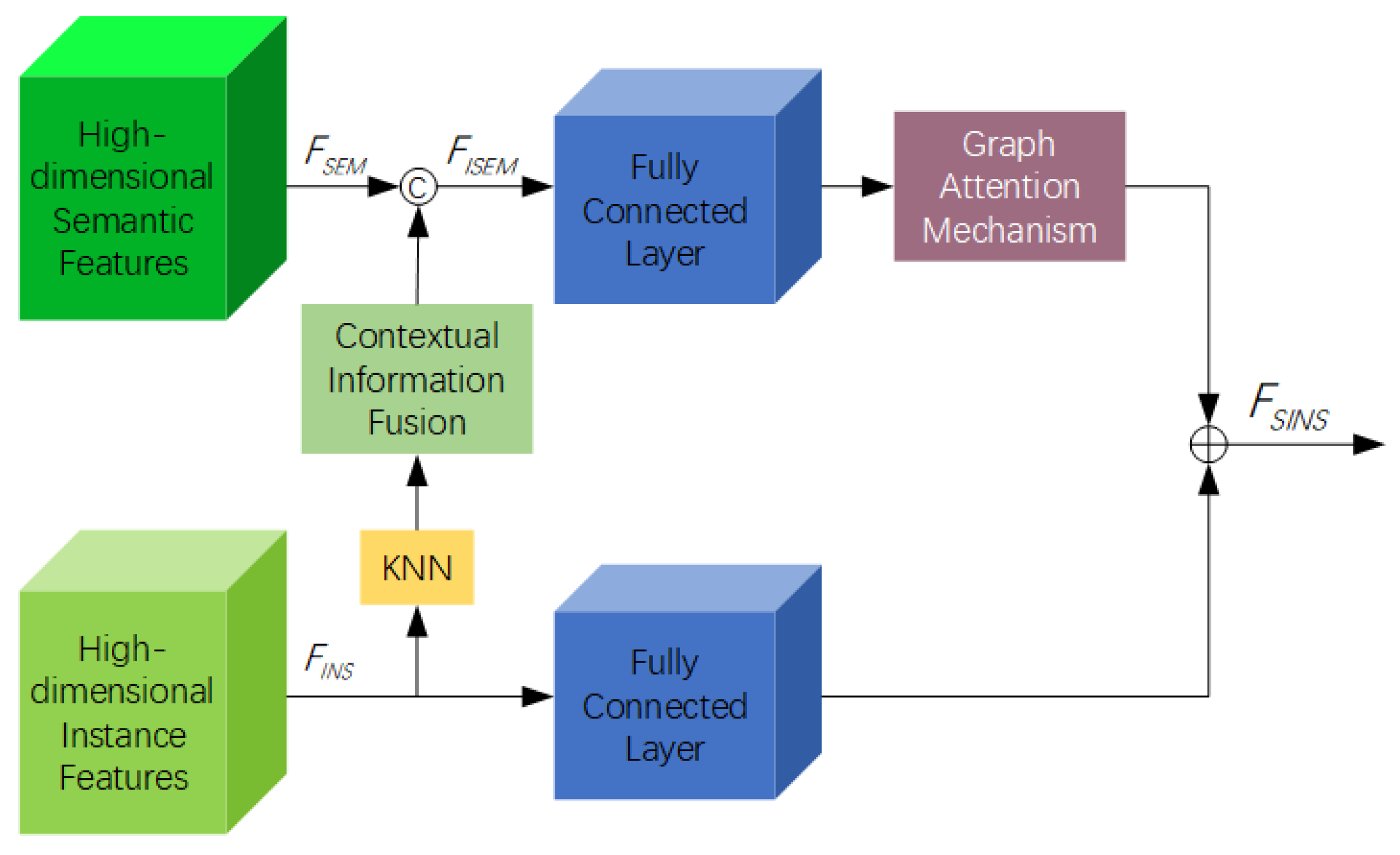
As shown in Figure 4, K-nearest neighbor search is adopted to find a fixed number of adjacent points for each point in the high-dimensional instance embedding space. We use k nearest neighbor search to generate the index matrix of the shape N a × K . According to the generated index matrix, we use the context information fusion module to generate the local neighborhood feature matrix of the instance space. In the semantic space, the feature tensor with the shape of N a × K × N F is generated according to the index matrix, and each group corresponds to the local region near a centroid in the instance embedding space. Through Equation (5), we equalize the local examples and semantic features to each dimensional feature to enhance the semantics and examples of centroid refinement.
x i = M e a n x i 1 , , x i K ,
where x i 1 , , x i K represents the semantic and instance fusion features corresponding to K adjacent points centered on point i in the instance embedding space.
In the enhanced high-dimensional semantic space, we construct a local neighborhood graph through K-nearest neighbors and use the graph attention mechanism to select more representative semantic features to enrich case features. The F = f 1 , f 2 , , f k and F R k × m are local neighborhood feature of each node is input into the graph attention module. m is the dimension of the feature, and k is the number of nodes. First of all, we encode the input context feature matrix through the shared weight matrix W R m × m . Then, we normalize the encoded features through the Softmax activation function to obtain the self-attention coefficient corresponding to the feature matrix of each node, F, as shown in Equation (7), e i j represents the influence of each neighborhood point feature on the node feature. Attention matrix is generated as a i j , and the activation function needs to be applied before obtaining the nodes in the next layer. The final screening of more representative semantic enhancement information F = f 1 , f 2 , , f k , and F R k × m are shown in Equation (8).
e i j = α W × f ,
a i j = S o f t m a x e i j = e x p e i j j N i e x p e i j ,
F = σ j N i a i j w f j ,
We combine more representative semantic enhancement information with high-dimensional instance features to form the final high-dimensional instance feature discrimination matrix that combines semantic information and instance information to enhance each other.

3.2.3. Loss Function Based on Metric Learning

The loss function is the discriminant loss function used in metric learning, as shown below.
L = L p u l l + L p u s h + α L r e g ,
where L p u l l pulls embeddings close to the mean embedding of instance, while the L p u s h makes the mean embedding of different instances separated from each other. L r e g is the regularization item (Equation (10)), which makes the center of the instance close to the origin and keeps the gradient always active.
L r e g = 1 I i = 1 I μ i 1 ,
where μ i is the average embedding of tree instance.
For individual tree segmentation, L p u l l makes points on the same tree in the high-dimensional instance space close to its center, which is defined as follows:
L p u l l = 1 M m = 1 M 1 N m n = 1 N m μ m E n 1 δ v + 2 ,
where δ v is the penalty margin for the center point of each instance. When the distance between the point on a single tree and its center point is less than δ v , no penalty will be imposed. In addition, x + = m a x 0 , x ; 1 is the L 1 norm, M is the number of the road-side trees, N m refers to the number of points in instance i, E n represents the embedding of points in the tree instance.
As shown in Equation (12), L p u s h keeps the points of different trees away from each other. When the distance between the centers of two tree instances exceeds 2 δ d , no penalty will be imposed, so that instances can be freely distributed in space.
L p u s h = 1 M M 1 i = 1 M j = 1 M 2 δ d μ i μ j 1 + 2 ,
During the testing, the final instance labels are obtained by using a simple mean-shift clustering [75] on the high-dimensional embedded feature space.

3.3. Estimation of Living Vegetation Volume

Living Vegetation Volume (LVV) calculation is an important task of urban ecology because it can objectively and accurately describe the urban greenery quality and provide a reliable data foundation for the quantitative study on the mechanism of urban greenery ecological functions. Benefited from our high-quality instance segmentation results of road-side trees, the convex hull method is adopted to calculate LVV of urban roads.
It is necessary to extract the canopy point cloud to calculate the LVV of road-side trees. According to the definition of the principal direction in differential geometry, the direction corresponding to the minimum curvature is adopted as the principal direction of the tree point cloud. The main directions of leaf point clouds are messy, while the main directions of point clouds in the branches are basically coincident. Therefore, the normal vectors of the object points and adjacent points are used to construct a dense tangent circle and further calculate the main direction of the tree point cloud. After that, the tree canopy is extracted according to the axial distribution density and axial similarity of the trunk. At given point, we judge the axial distribution density in the cylinder constructed by this point. The axis of the cylinder is divided into n segments. The inner point of the cylinder is projected onto the axis. The ratio of the segment occupied by the projection point to n is the axial distribution density. The optimal threshold is 0.8. The included angle of each point in the cylinder is then calculated, which refers to the included angle between the main direction of each point in the cylinder and the main direction of the center point. The best threshold is 20°. Finally, the specific gravity of the effective point is calculated. Specifically, the effective point refers to the point that meets the conditions that the axial distribution density is greater than the density threshold and the included angle ratio is less than the included angle threshold. The ratio of these points to the number of points in the cylinder is needed. The optimal threshold is 0.8. After many tests, the height of the constructed cylinder is 10 times the average density of the point cloud, and the radius is 2 times the average density. When the axial distribution density is greater than 0.8, the included angle is less than 20°, and the specific gravity of the effective point is greater than 0.8, the constructed cylinder is considered the best cylinder approximation of the trunk point cloud. Then, the trunk point cloud is regionally grown until all the point clouds are processed. Finally, the region is merged to identify the trunk point cloud and remove the trunk point cloud to complete the canopy extraction.
From the perspective of dendrometry, the traditional LVV calculation takes the crown width and crown height as parameters and treats the crown as regular geometry [76]. However, most of the crown shapes are variable and have no specific regular shape, resulting in large errors. We calculate the LVV by the convex hull method and compare it with the traditional method and the platform method.

4. Experimental Results

4.1. Dataset Description

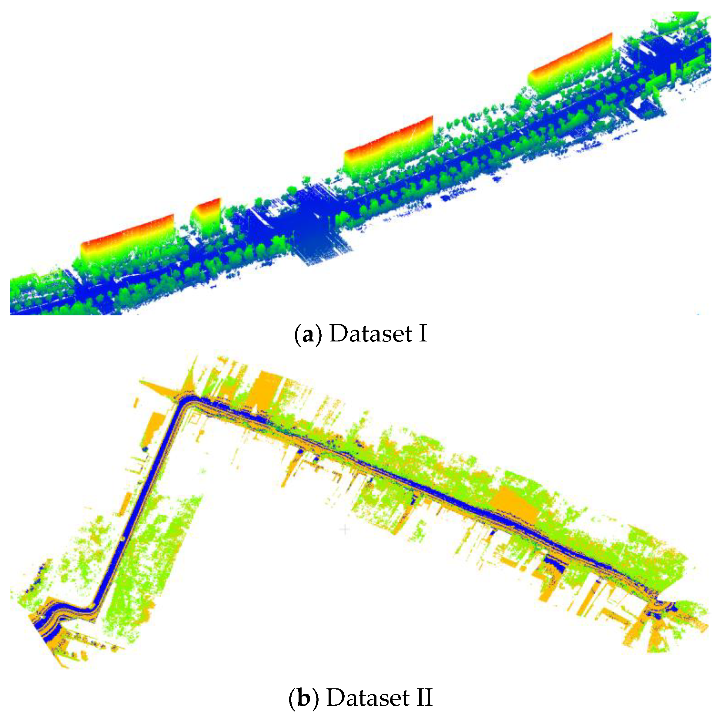
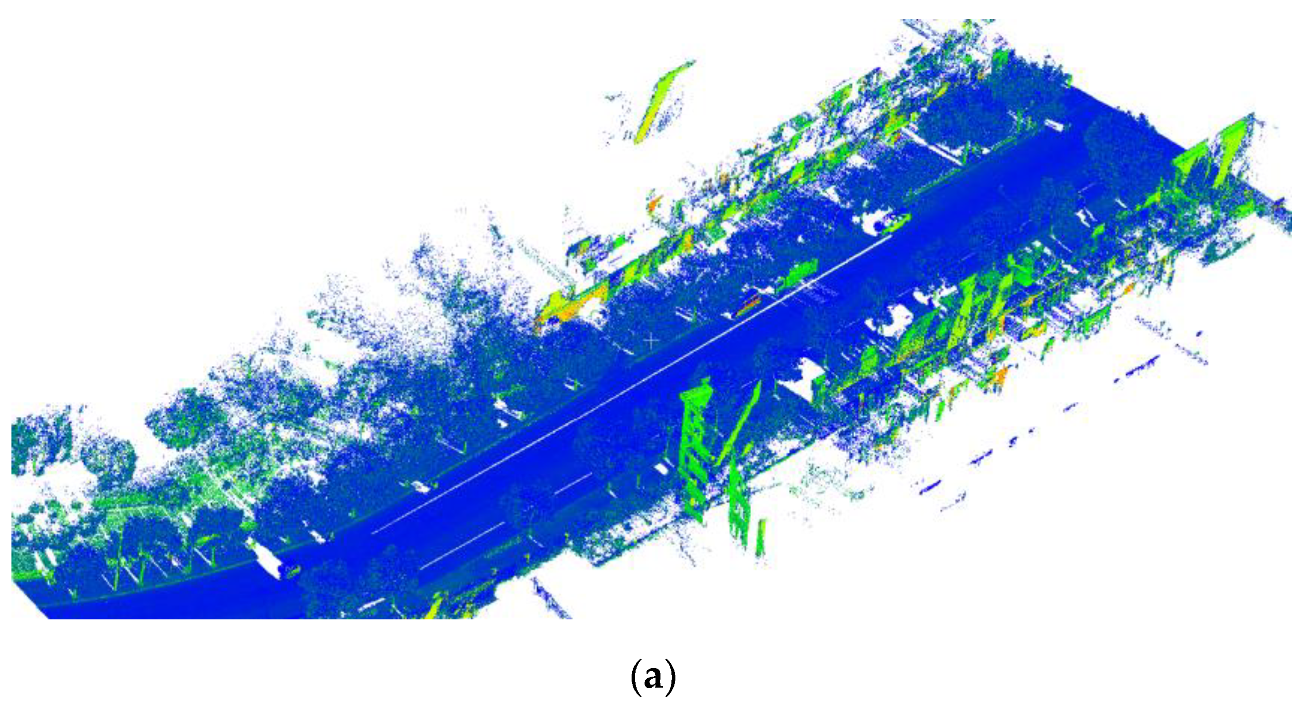
To check the performance of the proposed method, MLS point clouds from two different urban regions are used in the evaluation experiments. Dataset I was collected using a Riegl VMX-450 MLS system in the summer of 2020, covering approximately 6.0 km urban roads in Shanghai, China. Dataset II was collected using a Trimble MX2 MLS system in Nanjing, China, covering urban road length approximately 8.0 km. For training the neural network, 4.5 km of Dataset I and 6.0 km of Dataset II are manually labeled for quantitative evaluation. It is worth noting that the main characteristic of these two-point cloud datasets includes many road-side trees and the distributions of road-side trees presenting different situations. Figure 5 shows an overview of two urban MLS point cloud scenes. Several road-side trees are quite sparse, while others overlap heavily.

4.2. Semantic Segmentation Performances

4.2.1. Semantic Segmentation Results

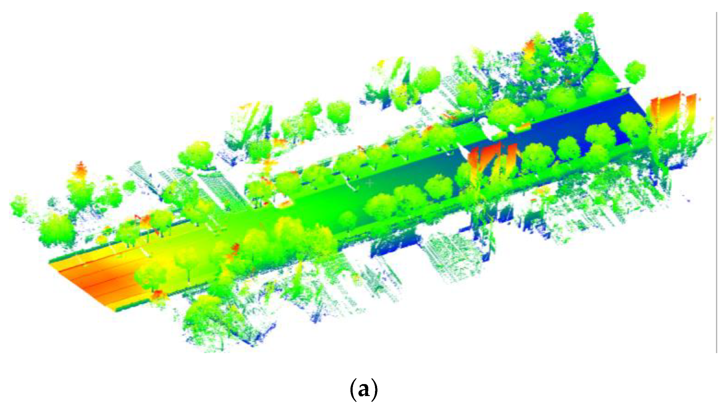
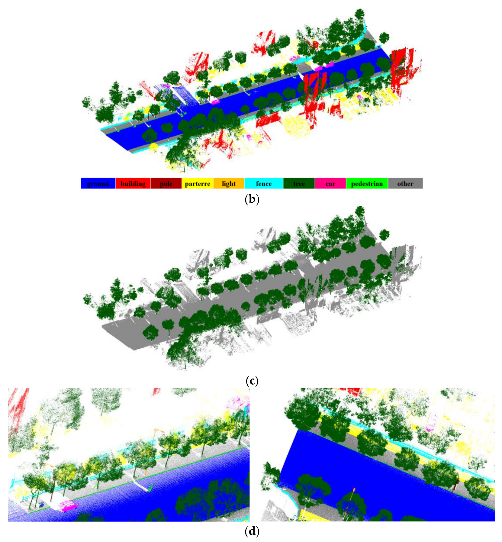
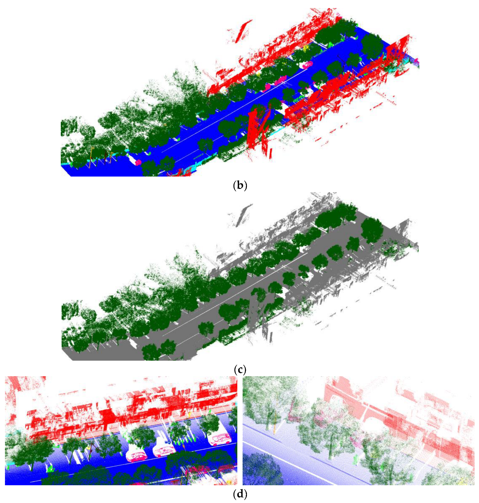
Figure 6 and Figure 7 illustrate the visual result by testing with selected point clouds from Dataset I and Dataset II, which verifies that our semantic segmentation model is able to achieve promising point-wise segmentation of the large-scale urban environments. Figure 6a and Figure 7a show the two selected MLS point clouds, colored by the elevation of each point. Figure 6b and Figure 7b present semantic segmentation outcomes, dotted in different colors according to the labels. After tree and non-tree points are identified by using semantic segmentation approach, the road-side trees are extracted from the raw urban MLS point cloud scenes. Figure 6c and Figure 7c illustrate the road-side tree extraction results, where the extracted road-side tree points are overlaid on the original urban MLS point clouds. To show more details of the road-side tree extraction outcomes, Figure 6d and Figure 7d present close-up results at some selected regions. Although MLS point clouds collected in urban roads are very complex, our semantic segmentation results indicate many objects (e.g., buildings and grounds) are effectively extracted, and the road-side trees are completely segmented.
To better present the urban MLS point cloud semantic segmentation performance of the proposed method, we quantitatively assess the semantic segmentation results in terms of the two commonly used evaluation metrics [20,41]: overall accuracy (OA) and mean intersection over union (mIoU). The numerical point cloud semantic segmentation results for Dataset I and Dataset II are listed in Table 1. As can be perceived, the proposed method achieves excellent performance in semantically segmenting MLS point clouds with an average OA and mIoU of (89.1%, 63.8%) and (88.8%, 64.3%) for the two MLS point cloud datasets, respectively. From the global perspective, the OAs of Dataset I and Dataset II exceed 88%, which demonstrates the effectiveness of our semantic segmentation model. Meanwhile, the OAs and mIoUs of Dataset I and Dataset II show no evident performance differences. Moreover, the IoU of road-side trees, the most important urban objects, surpass 87% in both Dataset I and Dataset II, achieving the ideal results for tree point extraction.

4.2.2. Comparison with Other Published Methods

For further semantic segmentation performance evaluation, we compare our semantic segmentation model with existing published networks obtaining baseline results. These networks can be viewed as reference methods, including PointNet++ [39], TagentConv [77], MS3_DVS [78], SPGraph [41], KPConv [40], RandLA-Net [44], and MS-RRFSegNet [20]. Specifically, PointNet++ [39] is a follow-up work of PointNet [38], which is the pioneer work directly on irregular points. It grouped points hierarchically and progressively acquired both local and global features. TagentConv [77] is a representative model of projection-based methods for semantic segmentation of large scenes. It introduced a novel tangent convolution and operated directly on precomputed tangent planes. MS3_DVS [78] is a representative model of discretization-based methods, which proposed multi-scale voxel network architecture to classify 3D point clouds of large scene. SPGraph [41] is one of the first methods capable of directly processing large-scale point clouds based on an attributed directed graph, which consists of geometrically homogeneous partitioning, super-point embedding, and contextual segmentation. KPConv [40] is a flexible point-wise convolution operator for point cloud semantic segmentation, which proposed a kernel point fully convolutional network to achieve state-of-the-art performance on the existing benchmarks. RandLA-Net [44] is a lightweight yet efficient point cloud semantic segmentation network, which utilized random point sampling to achieve vastly high efficiency and captured geometric features by a local feature aggregation module. MS-RRFSegNet [20] is a multiscale regional relation feature segmentation network, which adopted a sparse auto-encoder for feature embedding representations of the homogeneous super-voxels that reorganized raw data, and semantically labeled super-voxels based on the regional relation feature reasoning module.
For fair comparison, we faithfully follow the experimental settings of each selected algorithm that has available code. In addition, the proposed model is also compared between the Dataset I and Dataset II. All experiments are performed on a computer equipped with two NVIDIA GEFORCE RTX 3080 GPUs. Based on the same configurations, the quantitative results on the Dataset I and Dataset II are also presented in Table 1. As can be perceived, TagentConv [77] has the worst performance since the orientation of the tangent plane may not be estimated well in urban road scenes with topographic relief variations. The mIoU scores of the proposed method is the highest at present and is followed by RandLA-Net [44] with a gap of approximately 2%, while the KPConv [40] is slightly inferior to RandLA-Net [44] by approximately 0.4%, and SPGraph [41] achieves the fourth highest performance. It is worth noting that the abovementioned four methods are greatly superior to others in general. There are a number of common categories such as ground, vegetation, and building that are finely segmented due to the abundance of points of these categories in the dataset. In general, while the proposed method achieves satisfying semantic segmentation results and ranks highly, the overall segmentation performances of other state-of-the-art deep-learning methods are far from satisfactory. In particular, some key elements of road infrastructures have weak performances across all of the techniques.

4.3. Individual Tree Segmentation Perfromances

4.3.1. Tree Segmentation Results

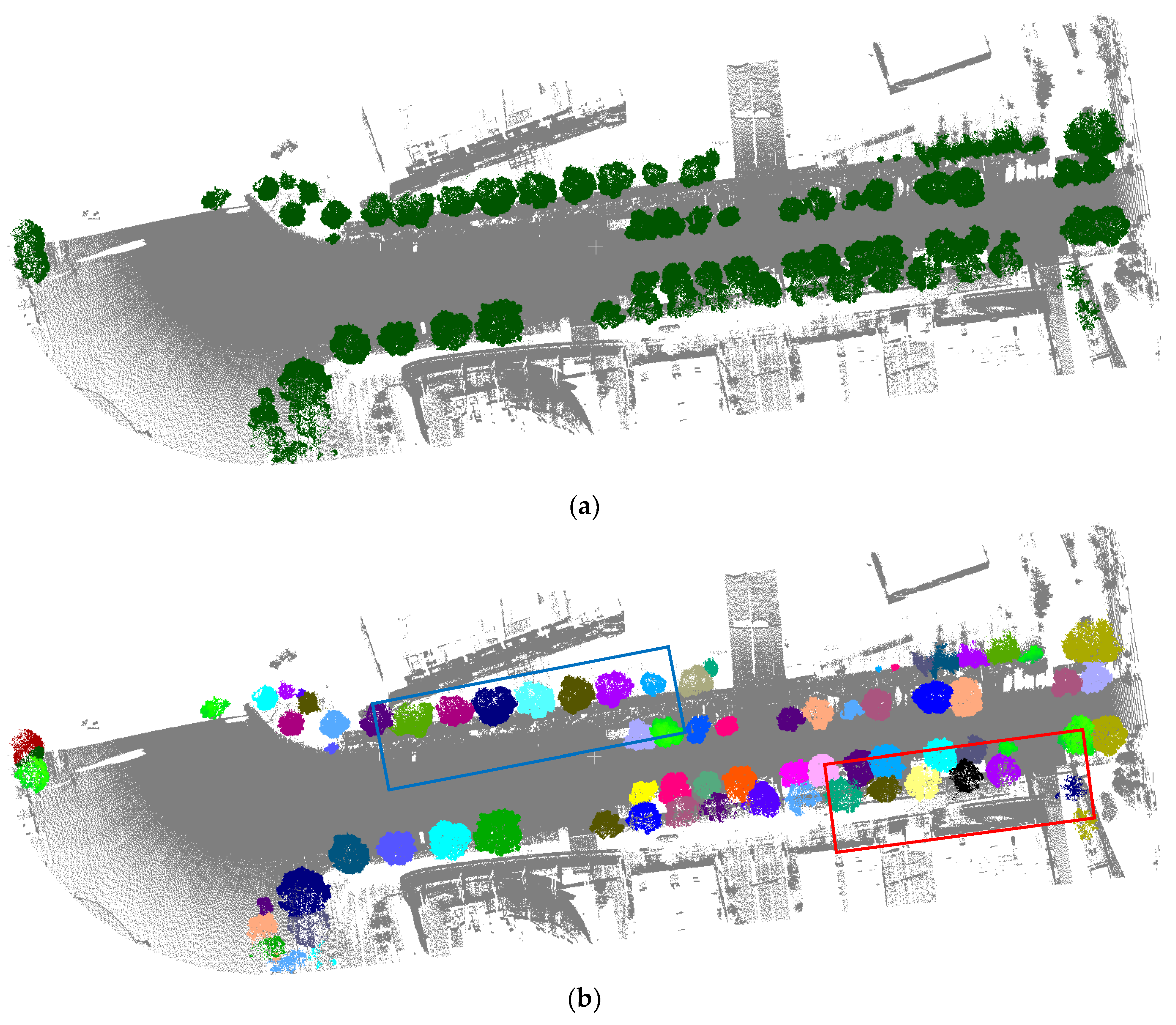
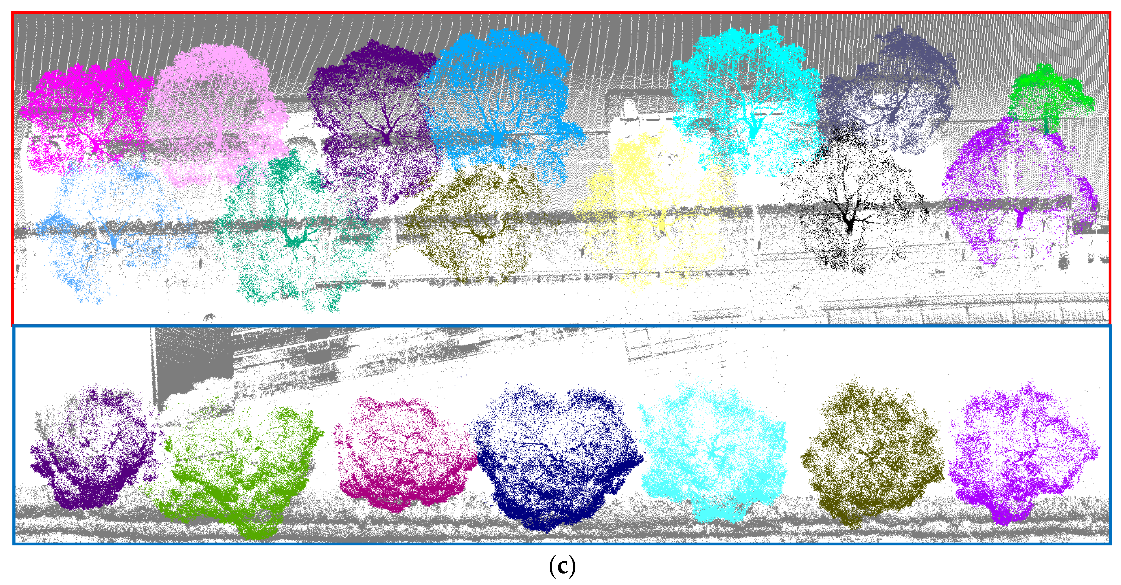
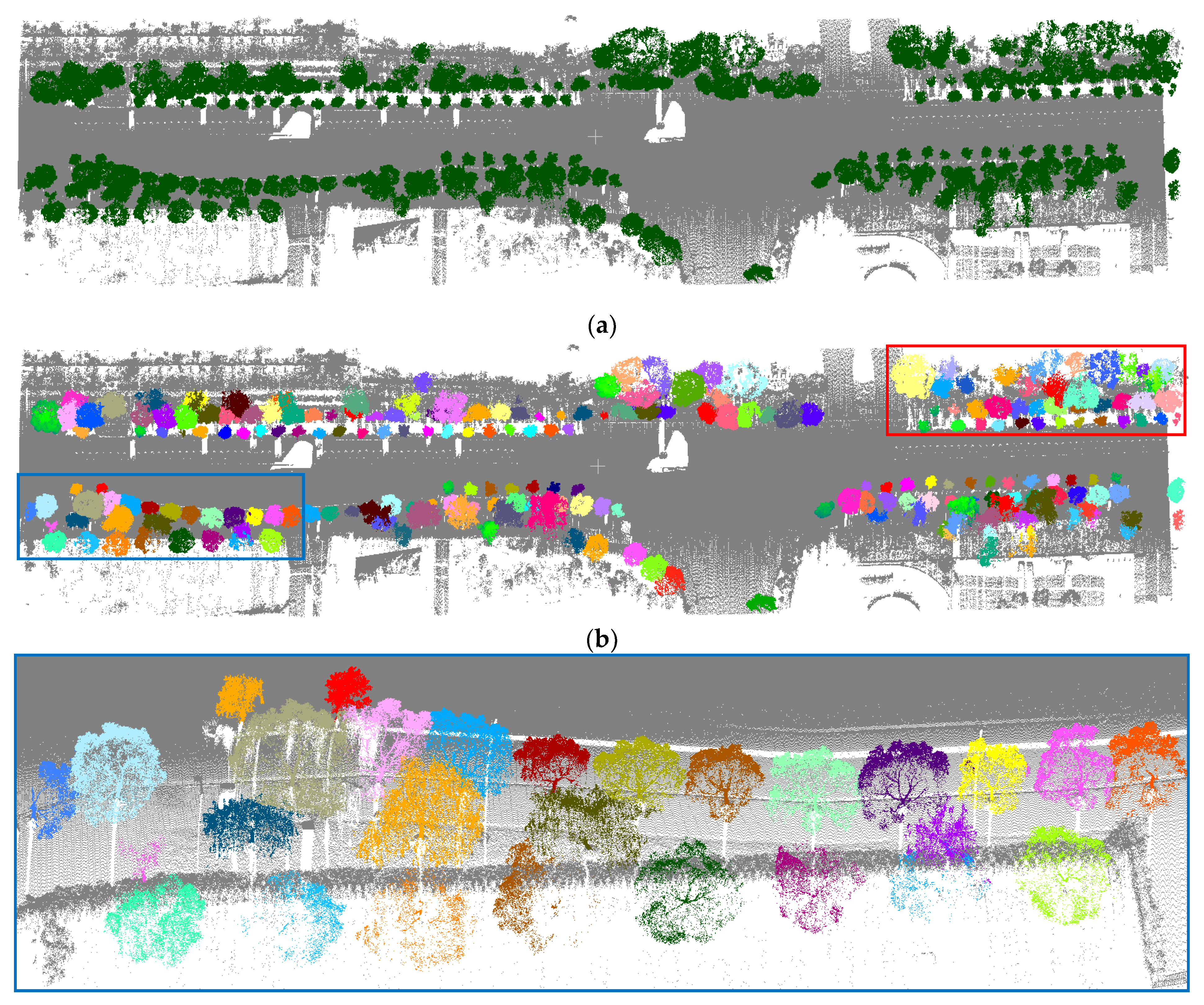
The individual tree segmentation performances of two urban MLS point clouds are estimated qualitatively. The visual samples in Figure 8 and Figure 9 are selected with different spatial structures of complex urban environments to show the good segmentation ability of the proposed method. Figure 8a and Figure 9a illustrate the road-side tree extraction results, where the extracted road-side tree points are overlaid on the original urban MLS point clouds. Figure 8b and Figure 9b present individual tree segmentation outcomes, where every road-side tree is drawn in one color. Figure 8c and Figure 9c show some zoom-in views of the individual tree segmentation results at some randomly selected regions. We can see that there exist some errors in the boundary regions of segmented instance-level road-side trees; nonetheless, it still has a high sensitivity to separate individual road-side trees.
To better show the individual tree segmentation results of the proposed method, we quantitatively evaluate the individual tree segmentation performances in terms of the four commonly used instance segmentation evaluation metrics [79]: the precision (Prec), the recall (Rec), the mean coverage (mCov) and the mean weighted coverage (mWCov) (see Equations (13)–(16)). The numerical instance segmentation results for Dataset I and Dataset II are presented in Table 2, respectively. We can see that the proposed method obtains good performance in individual tree segmentation from urban MLS point clouds with average mPrec, mRec, mCov and mWCov of (90.27%, 89.75%, 86.39%, 88.98%) and (90.86%, 89.27%, 87.20%, 88.56%) for the two urban MLS point cloud datasets, respectively. From the global perspective, the mPrec and mRec of Dataset I and Dataset II both exceed 89%, which demonstrates the effectiveness of the proposed individual tree segmentation network. Moreover, the mCov and mWCov of the instance segmentation of road-side trees surpass 86% and 88% in Dataset I and Dataset II, respectively, achieving the significant performances for individual tree segmentation from urban MLS point clouds. Meanwhile, these four instance-level metrics of Dataset I and Dataset II show no evident performance differences.
P r e c = T P i n s P i n s ,
R e c = T P i n s G i n s ,
where T P i n s represents the number of segmented road-side tree instances with an IoU with ground truth larger than 0.5; P i n s refers to the total number of predicted instances of the road-side trees, and G i n s indicates the number of the segmented road-side tree instances in the ground truth.
m C o v I , P = 1 I a = 1 I max b I o U I a , P b ,
m W C o v I , P = a = 1 I I a c = 1 I I c max b I o U I a , P b ,
where I represents the number of all road-side tree instances in the ground truth. I a indicates the a-th road-side tree instance area in the ground truth road-side tree instance collection, P b refers to the b-th segmented road-side tree instance area, b refers to the number of trees in the point cloud to be processed.

4.3.2. Comparative Studies

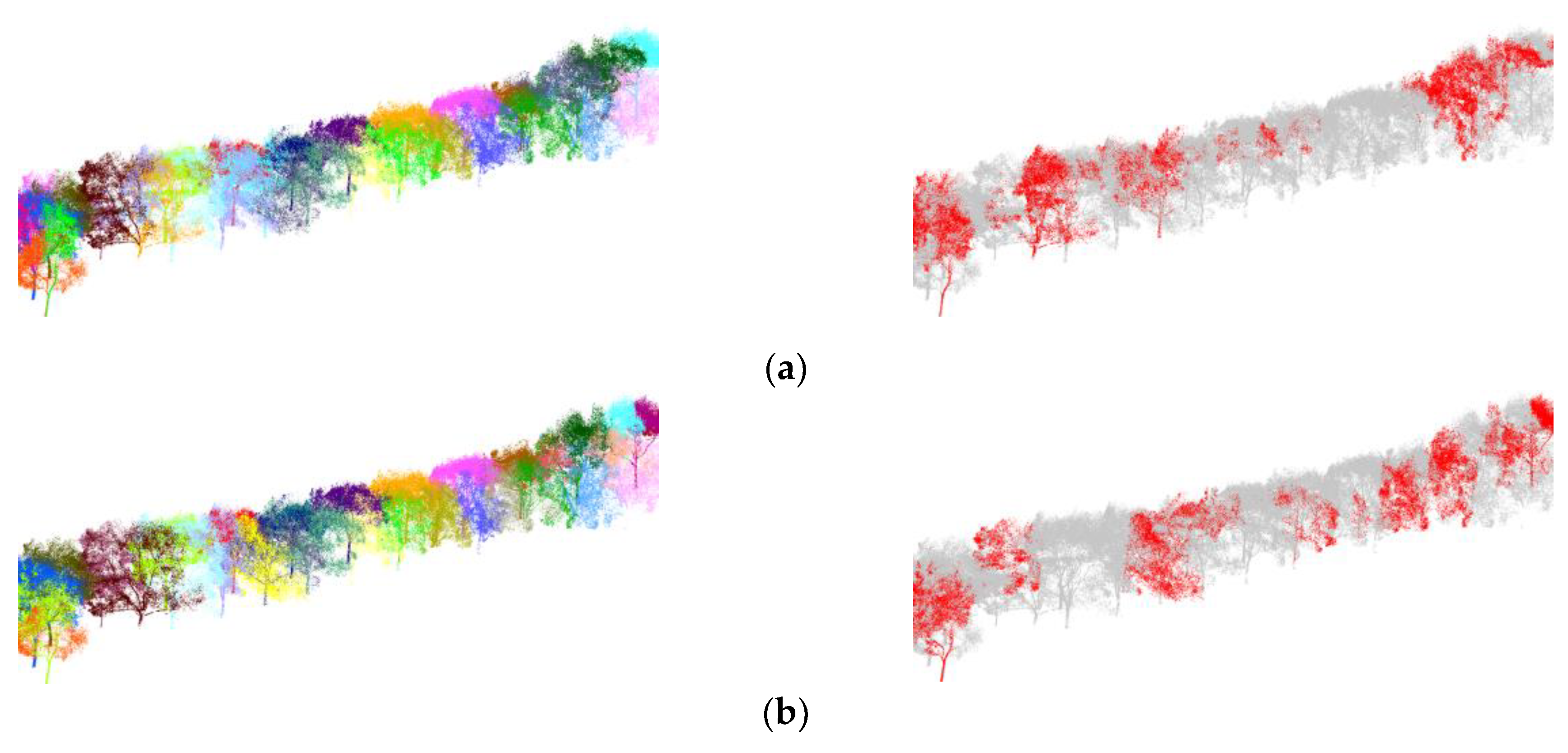
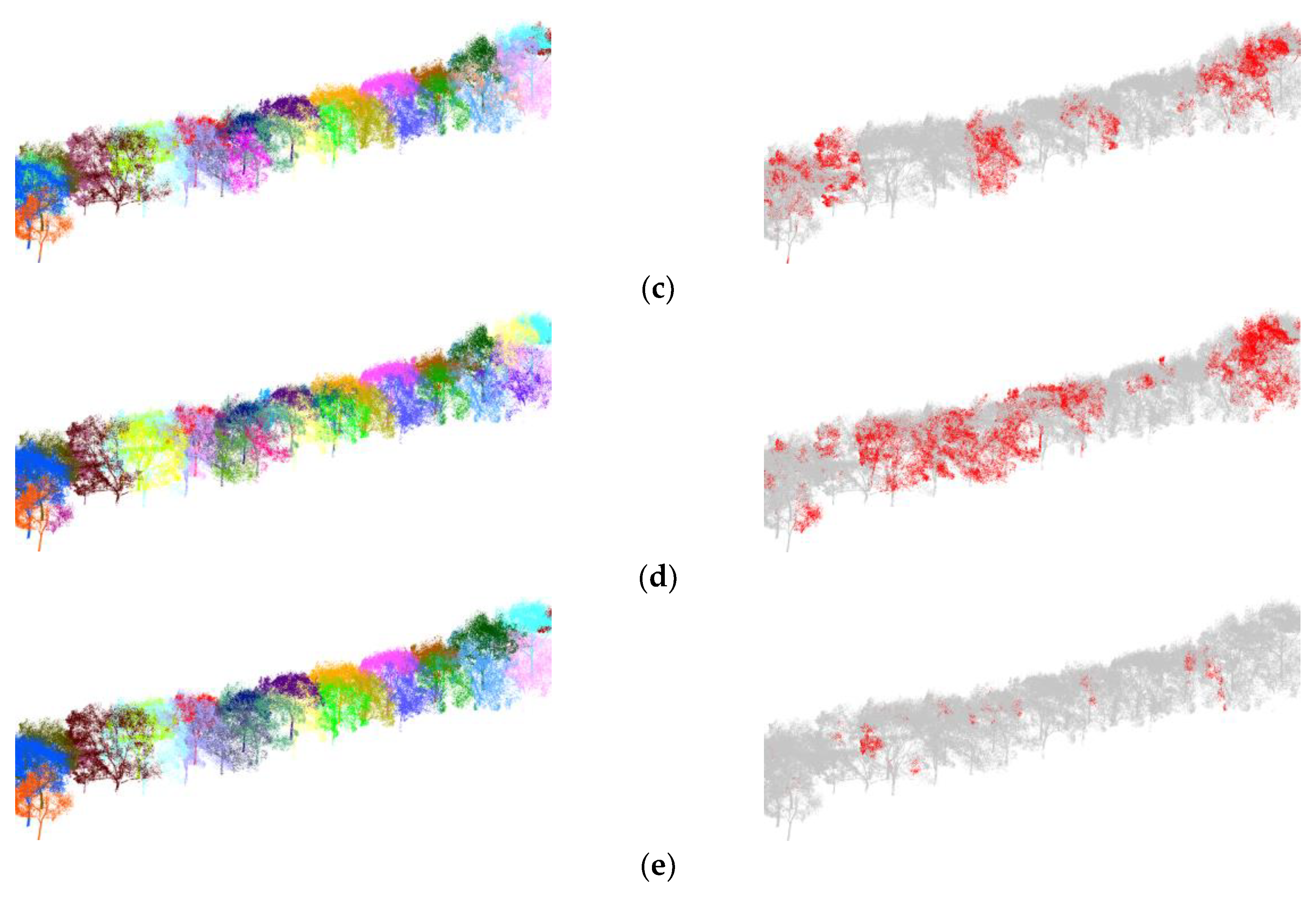
To further prove the superiority of our individual tree segmentation method, we designed a number of experiments and compared it with selected popular methods, including two traditional methods (watershed-based method [80] and mean shift-based method [81]) and two deep learning approaches (SGE_Net [64] and DAE_Net [67]). To qualitatively present the effectiveness of the proposed method for individual tree segmentation in complex urban MLS point cloud scenes, a selected examples of visual results are shown in Figure 10. Specifically, we can see that all methods obtain satisfactory results for road-trees with consistent tree shapes in simple situations. With regard to the complex position distribution, such as multiple trees distributed in a queue with serious spatial overlap, two traditional methods [80,81] are fast and efficient but easy to result in omission or commission errors. By contrast, two deep learning approaches [64,67] and our method can achieve better tree segmentation results. The main reason is that the traditional methods strongly depend on the boundary spatial features between adjacent road-side trees and the fixed shape assumption of road-side trees. For the deep learning methods based on the designed neural networks, their layer structure and parameters can implicitly express the spatial interactions between tree point clouds, facilitating the feature representations for instance segmentation. Although the deep learning methods introduce additional computational complexity, this degeneration should be tolerated when we conduct the individual tree segmentation in large-scale MLS point clouds.
Furthermore, since it is relatively limited to show the advantages of the proposed method by visual presentation, we further quantitatively compare the individual tree segmentation performance of four selected baselines and the proposed method. The numerical comparisons are also provided in Table 2 for Dataset I and Dataset II. The quantitative comparison for individual tree segmentation among four baselines shows that the proposed method achieves the best segmentation results on all four evaluation indicators, mPrec, mRec, mCov, and mWCov, not only for Dataset I but also for the Dataset II. As can be perceived, the mPrec, mRec, mCov, and mWCov of [80] are the worst at present and are followed by [81] with gaps of approximately 1.67%, 1.15%, 2.64%, and 2.69%, while the SGE_Net [64] is superior to DAE_Net [67] by approximately 2.30%, 1.99%, 1.10%, and 1.34%. Because DAE_Net [67] propose to use the pointwise direction embedding to distinguish the fine boundaries of individual road-side trees, it has more obvious improvements, compared to [80,81], and SGE_Net [64], on both two urban MLS point cloud datasets, which reveals that SGE_Net [64] is good at the individual tree segmentation task of the complex urban scenes. In practical application, however, there are inevitably errors in the detected tree centers. Therefore, from the comparison results of Table 2, we can see that SGE_Net [64] is slightly inferior to ours in general. For example, the proposed method outperforms the SGE_Net [64] by average improvements of approximately 3.24% in mPrec, approximately 2.63% in mRec, approximately 1.59% mCov, and more than 1.96% in mWCov. To sum up, it is evident that the proposed method has obtained a prominent improvement compared with the selected four reference baselines.

4.4. LVV Calculatation Results

It can be seen from Table 3, the relative error ( δ 1 ) between the adopted scheme and the traditional method is 12.6~33.7%, and the average relative error is 16.5~19.9%. The trees in the real urban scene are complex and changeable, and even the same tree species have different crown shapes. This situation leads to the fact that the true canopy profile of trees cannot be effectively expressed, so it is difficult to find the most suitable crown shape. In addition, due to the influence of human factors in the visual process, the error is large. The relative error ( δ 2 ) between the adopted scheme and the platform method is 2.7~14.6%, and the average relative error is 7.8~8.9%. The platform method does not need to consider the tree shape to calculate the LVV, which reduces the influence of human factors and improves the calculation efficiency. However, there is a large gap between the bottom layer and the bottom layer of the actual tree crown in the calculation of the platform method, resulting in a large error at the bottom layer. The calculation of the adopted scheme is based on high-precision tree point clouds, and the used convex polyhedron approximates the original shape of the tree crown, which can better express the space volume occupied by the tree stem and leaf. Therefore, the obtained LVV is more accurate and does not need to consider the tree shape, realizing the automatic calculation of LVV.
To better reflect the accuracy of LVV calculation, the correlation coefficient ( R 2 ) is adopted to compare the results of manual measurements and that from LVV calculated in the proposed model. The definition of the evaluation indicator is as follows:
R 2 = 1 q = 1 Q m q m q 2 q = 1 Q m q m ¯ q 2 ,
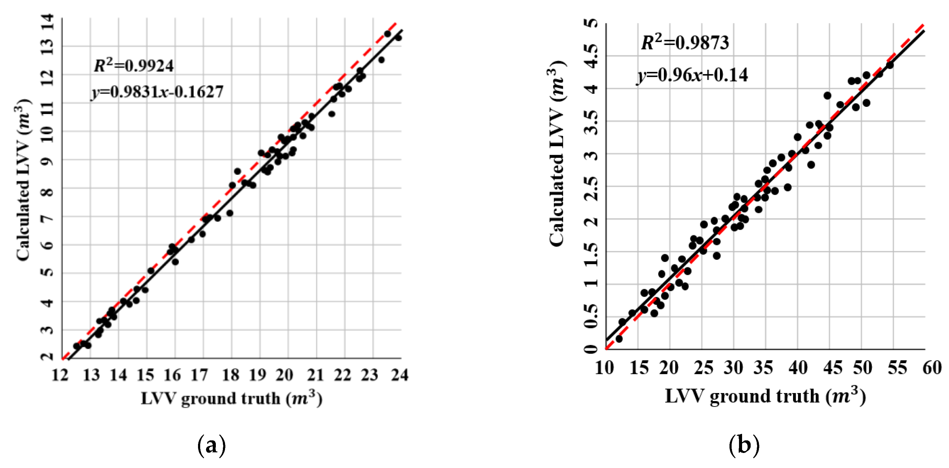
where Q denotes the number of trees; m q is the value of the manual measured LVV; m q is the value of LVV determined from the segmented tree point clouds; and m ¯ q is the mean value of the manually measured LVV. To evaluate the accuracy of the calculated LVVs based on the segmentation results of the proposed method, the calculated results are compared with manual measured ground truths. The linear correlations between calculated values and the manual measurements are given in Figure 11.
In the comparative results, R 2 of Dataset I and Dataset II are 0.9924 and 0.9873, respectively. The R 2 of two-point cloud datasets are close to 1, showing the correlation for tree-level LVV is high. Two fitted lines are close to y = x, showing high accuracies of our approach to extract instance-level road-side trees.

4.5. Generalization Capability

To further show the generalization ability of our approach, an additional experiment is carried out on an urban ALS point cloud dataset captured in Wuhan, China. This dataset is a highly dense ALS point cloud dataset with various types of urban objects, covering approximately 3.5 km2. The individual tree segmentation result is presented in Figure 12, proving that our method achieved good segmentation results on the ALS point clouds. Moreover, SGE_Net [64] and DAE_Net [67] are selected as comparison methods, and the corresponding individual tree segmentation results are provided in Table 4. The proposed method outperformed the above two deep learning methods, which obtained an average improvement of 5.56%, 3.58%, 4.78%, and 6.74% in terms of all mPrec, mRec, mCov, and mWCov scores, respectively.

5. Conclusions

The accurate individual tree segmentation is one of most important eco-urban construction tasks. In this study, a novel top-down framework is developed to extract individual tree from MLS point clouds by integrating semantic and instance segmentation. In various highway scenes, there are a large number of overlapping and irregular road-side trees in urban roads. The semantic segmentation network is first used to semantically segment tree points from raw point clouds. Next, an instance segmentation network is developed to isolate individual road-side trees. The instance segmentation network consists of a shared feature encoder, two parallel feature decoders, and a feature fusion module. To improve network accuracy and efficiency, the loss function based on metric learning is adopted for training. The Prec, Rec, mCov, and mWCov of (90.27%, 89.75%, 86.39%, and 88.98%, respectively) and (90.86%, 89.27%, 87.20%, and 88.56%, respectively) are obtained from two different MLS point cloud datasets. The achieved individual tree segmentation results are superior to that of other published methods. Individual tree segmentation results provide support for future eco-city analysis, such as calculating the LVV of urban roads. In conclusion, our work offers an effective solution to individual tree segmentation.

Author Contributions

Conceptualization, P.W., Y.T. and T.J.; methodology, P.W., Y.T. and T.J.; software, P.W., Y.T., Z.L., L.D. and T.J.; validation, L.D., S.L. and T.J.; formal analysis, Z.L., Y.Y., L.D., S.L. and T.J.; investigation, P.W., L.D. and T.J.; resources, P.W., Y.T., Y.Y., L.D., S.L. and T.J.; data curation, P.W., Y.T. and T.J.; writing—original draft preparation, P.W., Y.T., Z.L., L.D., S.L. and T.J.; writing—review and editing, P.W., Y.T., Z.L., L.D., S.L. and T.J.; visualization, Y.Y., L.D., S.L. and T.J.; supervision, S.L. and T.J.; project administration, P.W., Y.T. and T.J.; funding acquisition, P.W., Y.T. and T.J. All authors have read and agreed to the published version of the manuscript.

Funding

This research described in this paper was jointly funded by the National Natural Science Foundation of China under Grant 41771439 and the Postgraduate Research and Practice Innovation Program of Jiangsu Province under Grant KYCX18_1206.

Data Availability Statement

Data underlying the results presented in this paper are not publicly available at this time but may be obtained from the authors upon reasonable request.

Acknowledgments

The authors acknowledge the all reviewers for their valuable comments.

Conflicts of Interest

The authors declare no conflict of interest.

References

  1. Huo, L.; Lindberg, E.; Holmgren, J. Towards low vegetation identification: A new method for tree crown segmentation from LiDAR data based on a symmetrical structure detection algorithm (SSD). Remote Sens. Environ. 2022, 270, 112857. [Google Scholar] [CrossRef]
  2. Cheng, L.; Zhang, F.; Li, S.; Mao, J.; Xu, H.; Ju, W.; Liu, X.; Wu, J.; Min, K.; Zhang, X.; et al. Solar energy potential of urban buildings in 10 cities of China. Energy 2020, 196, 117038. [Google Scholar] [CrossRef]
  3. Lan, H.; Gou, Z.; Xie, X. A simplified evaluation method of rooftop solar energy potential based on image semantic segmentation of urban streetscapes. Sol. Energy 2021, 230, 912–924. [Google Scholar] [CrossRef]
  4. Gong, F.; Zeng, Z.; Ng, E.; Norford, L.K. Spatiotemporal patterns of street-level solar radiation estimated using Google Street View in a high-density urban environment. Build. Environ. 2019, 148, 547–566. [Google Scholar] [CrossRef]
  5. Yang, B.; Dong, Z.; Liu, Y.; Liang, F.; Wang, Y. Computing multiple aggregation levels and contextual features for road facilities recognition using mobile laser scanning data. ISPRS J. Photogramm. Remote Sens. 2017, 126, 180–194. [Google Scholar] [CrossRef]
  6. Yun, T.; Jiang, K.; Li, G.; Eichhorn, M.P.; Fan, J.; Liu, F.; Chen, B.; An, F.; Cao, L. Individual tree crown segmentation from airborne LiDAR data using a novel Gaussian filter and energy function minimization-based approach. Remote Sens. Environ. 2021, 256, 112307. [Google Scholar] [CrossRef]
  7. Jiang, T.; Liu, S.; Zhang, Q.; Zhao, L.; Sun, J.; Wang, Y. ShrimpSeg: A local-global structure for mantis shrimp point cloud segmentation network with contextual reasoning. Appl. Opt. 2023, 62, 97–103. [Google Scholar] [CrossRef]
  8. Jiang, T.; Wang, Y.; Liu, S.; Cong, Y.; Dai, L.; Sun, J. Local and global structure for urban ALS point cloud semantic segmentation with ground-aware attention. IEEE Trans. Geosci. Remote Sens. 2022, 60, 5702615. [Google Scholar] [CrossRef]
  9. Liu, X.; Chen, Y.; Li, S.; Cheng, L.; Li, M. Hierarchical Classification of Urban ALS Data by Using Geometry and Intensity Information. Sensors 2019, 19, 4583. [Google Scholar] [CrossRef] [Green Version]
  10. Wang, Y.; Jiang, T.; Yu, M.; Tao, S.; Sun, J.; Liu, S. Semantic-Based Building Extraction from LiDAR Point Clouds Using Contexts and Optimization in Complex Environment. Sensors 2020, 20, 3386. [Google Scholar] [CrossRef]
  11. Lei, X.; Guan, H.; Ma, L.; Yu, Y.; Dong, Z.; Gao, K.; Delavar, M.R.; Li, J. WSPointNet: A multi-branch weakly supervised learning network for semantic segmentation of large-scale mobile laser scanning point clouds. Int. J. Appl. Earth Obs. Geoinf. 2022, 115, 103129. [Google Scholar] [CrossRef]
  12. Hu, T.; Wei, D.; Su, Y.; Wang, X.; Zhang, J.; Sun, X.; Liu, Y.; Guo, Q. Quantifying the shape of urban street trees and evaluating its influence on their aesthetic functions based on mobile lidar data. ISPRS J. Photogramm. Remote Sens. 2022, 184, 203–214. [Google Scholar] [CrossRef]
  13. Yang, B.; Dai, W.; Dong, Z.; Liu, Y. Automatic Forest Mapping at Individual Tree Levels from Terrestrial Laser Scanning Point Clouds with a Hierarchical Minimum Cut Method. Remote Sens. 2016, 8, 372. [Google Scholar] [CrossRef] [Green Version]
  14. Klouček, T.; Klápště, P.; Marešová, J.; Komárek, J. UAV-Borne Imagery Can Supplement Airborne Lidar in the Precise Description of Dynamically Changing Shrubland Woody Vegetation. Remote Sens. 2022, 14, 2287. [Google Scholar] [CrossRef]
  15. Liu, J.; Skidmore, A.K.; Wang, T.; Zhu, X.; Premier, J.; Heurich, M.; Beudert, B.; Jones, S. Variation of leaf angle distribution quantified by terrestrial LiDAR in natural European beech forest. ISPRS J. Photogramm. Remote Sens. 2019, 148, 208–220. [Google Scholar] [CrossRef]
  16. Moudrý, V.; Gdulová, K.; Fogl, M.; Klápště, P.; Urban, R.; Komárek, J.; Moudrá, L.; Štroner, M.; Barták, V.; Solský, M. Comparison of leaf-off and leaf-on combined UAV imagery and airborne LiDAR for assessment of a post-mining site terrain and vegetation structure: Prospects for monitoring hazards and restoration success. Appl. Geogr. 2019, 104, 32–41. [Google Scholar] [CrossRef]
  17. Wang, D.; Takoudjou, S.M.; Casella, E. LeWoS: A universal leaf-wood classification method to facilitate the 3D modelling of large tropical trees using terrestrial LiDAR. Methods Ecol. Evol. 2020, 11, 376–389. [Google Scholar] [CrossRef]
  18. Zou, Y.; Weinacker, H.; Koch, B. Towards Urban Scene Semantic Segmentation with Deep Learning from LiDAR Point Clouds: A Case Study in Baden-Württemberg, Germany. Remote Sens. 2021, 13, 3220. [Google Scholar] [CrossRef]
  19. Jiang, T.; Sun, J.; Liu, S.; Zhang, X.; Wu, Q.; Wang, Y. Hierarchical semantic segmentation of urban scene point clouds via group proposal and graph attention network. Int. J. Appl. Earth Obs. Geoinf. 2021, 105, 102626. [Google Scholar] [CrossRef]
  20. Luo, H.; Chen, C.; Fang, L.; Khoshelham, K.; Shen, G. MS-RRFSegNet: Multiscale regional relation feature segmentation network for semantic segmentation of urban scene point clouds. IEEE Trans. Geosci. Remote Sens. 2020, 58, 8301–8315. [Google Scholar] [CrossRef]
  21. Huang, R.; Xu, Y.; Stilla, U. GraNet: Global relation-aware attentional network for semantic segmentation of ALS point clouds. ISPRS J. Photogramm. Remote Sens. 2021, 177, 1–20. [Google Scholar] [CrossRef]
  22. Chen, Q.; Zhang, Z.; Chen, S.; Wen, S.; Ma, H.; Xu, Z. A self-attention based global feature enhancing network for semantic segmentation of large-scale urban street-level point clouds. Int. J. Appl. Earth Obs. Geoinf. 2022, 113, 102974. [Google Scholar] [CrossRef]
  23. Kang, Z.; Yang, J. A probabilistic graphical model for the classification of mobile LiDAR point clouds. ISPRS J. Photogramm. Remote Sens. 2018, 143, 108–123. [Google Scholar] [CrossRef]
  24. Li, Y.; Luo, Y.; Gu, X.; Chen, D.; Gao, F.; Shuang, F. Point Cloud Classification Algorithm Based on the Fusion of the Local Binary Pattern Features and Structural Features of Voxels. Remote Sens. 2021, 13, 3156. [Google Scholar] [CrossRef]
  25. Tong, G.; Li, Y.; Chen, D.; Xia, S.; Peethambaran, J.; Wang, Y. Multi-View Features Joint Learning with Label and Local Distribution Consistency for Point Cloud Classification. Remote Sens. 2020, 12, 135. [Google Scholar] [CrossRef] [Green Version]
  26. Zhang, Z.; Sun, L.; Zhong, R.; Chen, D.; Zhang, L.; Li, X.; Wang, Q.; Chen, S. Hierarchical Aggregated Deep Features for ALS Point Cloud Classification. IEEE Trans. Geosci. Remote Sens. 2020, 59, 1686–1699. [Google Scholar] [CrossRef]
  27. Lin, Y.; Vosselman, G.; Cao, Y.; Yang, M.Y. Local and global encoder network for semantic segmentation of Airborne laser scanning point clouds. ISPRS J. Photogramm. Remote Sens. 2021, 176, 151–168. [Google Scholar] [CrossRef]
  28. Yang, B.; Jiang, T.; Wu, W.; Zhou, Y.; Dai, L. Automated Semantics and Topology Representation of Residential-Building Space Using Floor-Plan Raster Maps. IEEE J. Sel. Top. Appl. Earth Observ. Remote Sens. 2022, 15, 7809–7825. [Google Scholar] [CrossRef]
  29. Yuan, Z.; Cheng, M.; Zeng, W.; Su, Y.; Liu, W.; Yu, S.; Wang, C. Prototype-Guided Multitask Adversarial Network for Cross-Domain LiDAR Point Clouds Semantic Segmentation. IEEE Trans. Geosci. Remote Sens. 2023, 61, 5700613. [Google Scholar] [CrossRef]
  30. Feng, H.; Chen, Y.; Luo, Z.; Sun, W.; Li, W.; Li, J. Automated extraction of building instances from dual-channel airborne LiDAR point clouds. Int. J. Appl. Earth Obs. Geoinf. 2022, 114, 103042. [Google Scholar] [CrossRef]
  31. Guo, Y.; Wang, H.; Hu, Q.; Liu, H.; Liu, L.; Bennamoun, M. Deep learning for 3D point clouds: A survey. IEEE Trans. Pattern Anal. Mach. Intell. 2021, 43, 4338–4364. [Google Scholar] [CrossRef] [PubMed]
  32. Yang, Z.; Jiang, W.; Xu, B.; Zhu, Q.; Jiang, S.; Huang, W. A convolutional neural network-based 3D semantic labeling method for ALS point clouds. Remote Sens. 2017, 9, 936. [Google Scholar] [CrossRef] [Green Version]
  33. Yang, Z.; Tan, B.; Pei, H.; Jiang, W. Segmentation and multiscale convolutional neural network-based classification of airborne laser scanner data. Sensors 2018, 18, 3347. [Google Scholar] [CrossRef] [PubMed] [Green Version]
  34. Lei, X.; Wang, H.; Wang, C.; Zhao, Z.; Miao, J.; Tian, P. ALS point cloud classification by integrating an improved fully convolutional network into transfer learning with multi-scale and multi-view deep features. Sensors 2020, 20, 6969. [Google Scholar] [CrossRef] [PubMed]
  35. Choy, C.; Gwak, J.; Savarese, S. 4D spatio-temporal convnets: Minkowski convolutional neural networks. In Proceedings of the IEEE Conference on Computer Vision and Pattern Recognition (CVPR), Long Beach, CA, USA, 16–20 June 2019; pp. 3075–3084. [Google Scholar]
  36. Zhang, J.; Hu, X.; Dai, H. A graph-voxel joint convolution neural network for ALS point cloud segmentation. IEEE Access 2020, 8, 139781–139791. [Google Scholar] [CrossRef]
  37. Qin, N.; Hu, X.; Wang, P.; Shan, J.; Li, Y. Semantic labeling of ALS point cloud via learning voxel and pixel representations. IEEE Geosci. Remote Sens. Lett. 2020, 17, 859–863. [Google Scholar] [CrossRef]
  38. Qi, C.R.; Su, H.; Kaichun, M.; Guibas, L.J. PointNet: Deep learning on point sets for 3D classification and segmentation. In Proceedings of the 2017 IEEE Conference on Computer Vision and Pattern Recognition (CVPR), Honolulu, HI, USA, 21–26 July 2017; pp. 652–660. [Google Scholar]
  39. Qi, C.R.; Yi, L.; Su, H.; Guibas, L.J. PointNet++: Deep hierarchical feature learning on point sets in a metric space. In Proceedings of the Advances in Neural Information Processing Systems, Long Beach, CA, USA, 4–9 December 2017; pp. 5099–5108. [Google Scholar]
  40. Thomas, H.; Qi, C.R.; Deschaud, J.-E.; Marcotegui, B.; Goulette, F.; Guibas, L. KPConv: Flexible and deformable convolution for point clouds. In Proceedings of the 2019 IEEE/CVF International Conference on Computer Vision (ICCV), Seoul, Korea, 27 October 2019–2 November 2019; pp. 6411–6420. [Google Scholar]
  41. Landrieu, L.; Simonovsky, M. Large-scale point cloud semantic segmentation with superpoint graphs. In Proceedings of the IEEE Conference on Computer Vision and Pattern Recognition, Salt Lake City, UT, USA, 18–23 June 2018; pp. 4558–4567. [Google Scholar]
  42. Chen, S.; Miao, Z.; Chen, H.; Mukherjee, M.; Zhang, Y. Point-attention Net: A graph attention convolution network for point cloud segmentation. Appl. Intell. 2022. [Google Scholar] [CrossRef]
  43. Zou, J.; Zhang, Z.; Chen, D.; Li, Q.; Sun, L.; Zhong, R.; Zhang, L.; Sha, J. GACM: A Graph Attention Capsule Model for the Registration of TLS Point Clouds in the Urban Scene. Remote Sens. 2021, 13, 4497. [Google Scholar] [CrossRef]
  44. Hu, Q.; Yang, B.; Xie, L.; Rosa, S.; Guo, Y.; Wang, Z.; Trigoni, N.; Markham, A. RandLA-Net: Efficient semantic segmentation of large-scale point clouds. In Proceedings of the IEEE Conference on Computer Vision and Pattern Recognition, Seattle, WA, USA, 13–19 June 2020; pp. 11105–11114. [Google Scholar]
  45. Hou, J.; Dai, A.; Nießner, M. 3D-SIS: 3D semantic instance segmentation of RGB-D scans. In Proceedings of the IEEE Conference on Computer Vision and Pattern Recognition, Long Beach, CA, USA, 15–20 June 2019; pp. 4416–4427. [Google Scholar]
  46. Yi, L.; Zhao, W.; Wang, H.; Sung, M.; Guibas, L.J. GSPN: Generative shape proposal network for 3D instance segmentation in point cloud. In Proceedings of the IEEE Conference on Computer Vision and Pattern Recognition, Long Beach, CA, USA, 15–20 June 2019; pp. 3942–3951. [Google Scholar]
  47. Yang, B.; Wang, J.; Clark, R.; Hu, Q.; Wang, S.; Markham, A.; Trigoni, N. Learning object bounding boxes for 3D instance segmentation on point clouds. In Proceedings of the Advances in Neural Information Processing Systems, Vancouver, BC, Canada, 8–14 December 2019; pp. 6737–6746. [Google Scholar]
  48. Engelmann, F.; Bokeloh, M.; Fathi, A.; Leibe, B.; Nießner, M. 3D-MPA: Multi-proposal aggregation for 3D semantic instance segmentation. In Proceedings of the IEEE Conference on Computer Vision and Pattern Recognition, Seattle, WA, USA, 13–19 June 2020; pp. 9028–9037. [Google Scholar]
  49. Jiang, L.; Zhao, H.; Shi, S.; Liu, S.; Fu, C.W.; Jia, J. Pointgroup: Dual-set point grouping for 3d instance segmentation. In Proceedings of the IEEE/CVF Conference on Computer Vision and Pattern Recognition, Seattle, WA, USA, 13–19 June 2020; pp. 4867–4876. [Google Scholar]
  50. Wang, X.; Liu, S.; Shen, X.; Shen, C.; Jia, J. Associatively segmenting instances and semantics in point clouds. In Proceedings of the IEEE Conference on Computer Vision and Pattern Recognition, Long Beach, CA, USA, 15–20 June 2019; pp. 4091–4100. [Google Scholar]
  51. Han, L.; Zheng, T.; Xu, L.; Fang, L. Occuseg: Occupancy-aware 3D instance segmentation. In Proceedings of the IEEE/CVF Conference on Computer Vision and Pattern Recognition, Seattle, WA, USA, 13–19 June 2020; pp. 2937–2946. [Google Scholar]
  52. Wang, Y.; Zhang, Z.; Zhong, R.; Sun, L.; Leng, S.; Wang, Q. Densely connected graph convolutional network for joint semantic and instance segmentation of indoor point clouds. ISPRS J. Photogramm. Remote Sens. 2021, 182, 67–77. [Google Scholar] [CrossRef]
  53. Chen, S.; Fang, J.; Zhang, Q.; Liu, W.; Wang, X. Hierarchical Aggregation for 3D Instance Segmentation. In Proceedings of the 2021 IEEE/CVF International Conference on Computer Vision (ICCV), Montreal, QC, Canada, 10–17 October 2021; pp. 15447–15456. [Google Scholar]
  54. Vu, T.; Kim, K.; Luu, T.M.; Nguyen, T.; Yoo, C.D. SoftGroup for 3D instance segmentation on point clouds. In Proceedings of the IEEE Conference on Computer Vision and Pattern Recognition, New Orleans, LA, USA, 18–24 June 2022; pp. 2698–3007. [Google Scholar]
  55. Chen, F.; Wu, F.; Gao, G.; Ji, Y.; Xu, J.; Jiang, G.; Jing, X. JSPNet: Learning joint semantic & instance segmentation of point clouds via feature self-similarity and cross-task probability. Pattern Recognit. 2022, 122, 108250. [Google Scholar]
  56. Chen, Y.; Wang, S.; Li, J.; Ma, L.; Wu, R.; Luo, Z.; Wang, C. Rapid urban roadside tree inventory using a mobile laser scanning system. IEEE J. Sel. Top. Appl. Earth Observ. Remote Sens. 2019, 12, 3690–3700. [Google Scholar] [CrossRef]
  57. Yang, J.; Kang, Z.; Cheng, S.; Yang, Z.; Akwensi, P.H. An individual tree segmentation method based on watershed algorithm and three-dimensional spatial distribution analysis from airborne LiDAR point clouds. IEEE J. Sel. Top. Appl. Earth Observ. Remote Sens. 2020, 13, 1055–1067. [Google Scholar] [CrossRef]
  58. Yan, W.; Guan, H.; Cao, L.; Yu, Y.; Li, C.; Lu, J. A self-adaptive mean shift tree-segmentation method using UAV LiDAR data. Remote Sens. 2020, 12, 515. [Google Scholar] [CrossRef] [Green Version]
  59. Dai, W.; Yang, B.; Dong, Z.; Shaker, A. A new method for 3D individual tree extraction using multispectral airborne LiDAR point clouds. ISPRS J. Photogramm. Remote Sens. 2018, 144, 400–411. [Google Scholar] [CrossRef]
  60. Yang, W.; Liu, Y.; He, H.; Lin, H.; Qiu, G.; Guo, L. Airborne LiDAR and photogrammetric point cloud fusion for extraction of urban tree metrics according to street network segmentation. IEEE Access 2021, 9, 97834–97842. [Google Scholar] [CrossRef]
  61. Xu, X.; Zhou, Z.; Tang, Y.; Qu, Y. Individual tree crown detection from high spatial resolution imagery using a revised local maximum filtering. Remote Sens. Environ. 2021, 258, 112397. [Google Scholar] [CrossRef]
  62. Windrim, L.; Bryson, M. Forest tree detection and segmentation using high resolution airborne LiDAR. In Proceedings of the IEEE/RSJ International Conference on Intelligent Robots and Systems (IROS), Macau, China, 3–8 November 2019; pp. 3898–3904. [Google Scholar]
  63. Mäyrä, J.; Keski-Saari, S.; Kivinen, S.; Tanhuanpää, T.; Hurskainen, P.; Kullberg, P.; Poikolainen, L.; Viinikka, A.; Tuominen, S.; Kumpula, T.; et al. Tree species classification from airborne hyperspectral and LiDAR data using 3D convolutional neural networks. Remote Sens. Environ. 2021, 256, 112322. [Google Scholar] [CrossRef]
  64. Wang, Y.; Jiang, T.; Liu, J.; Li, X.; Liang, C. Hierarchical instance recognition of individual roadside trees in environmentally complex urban areas from UAV laser scanning point clouds. ISPRS Int. J. GeoInf. 2020, 9, 595. [Google Scholar] [CrossRef]
  65. Chen, Y.; Wu, R.; Yang, C.; Lin, Y. Urban vegetation segmentation using terrestrial LiDAR point clouds based on point non-local means network. Int. J. Appl. Earth Obs. Geoinf. 2021, 105, 102580. [Google Scholar] [CrossRef]
  66. Luo, Z.; Zhang, Z.; Li, W.; Chen, Y.; Wang, C.; Nurunnabi, A.A.M.; Li, J. Detection of individual trees in UAV LiDAR point clouds using a deep learning framework based on multichannel representation. IEEE Trans. Geosci. Remote Sens. 2022, 60, 5701715. [Google Scholar] [CrossRef]
  67. Luo, H.; Khoshelham, K.; Chen, C.; He, H. Individual tree extraction from urban mobile laser scanning point clouds using deep pointwise direction embedding. ISPRS J. Photogramm. Remote Sens. 2021, 175, 326–339. [Google Scholar] [CrossRef]
  68. Jin, S.; Su, Y.; Zhao, X.; Hu, T.; Guo, Q. A point-based fully convolutional neural network for airborne LiDAR ground point filtering in forested environments. IEEE J. Sel. Top. Appl. Earth Obs. Remote Sens. 2020, 13, 3958–3974. [Google Scholar] [CrossRef]
  69. Zhao, X.; Guo, Q.; Su, Y.; Xue, B. Improved progressive TIN densification filtering algorithm for airborne LiDAR data in forested areas. ISPRS J. Photogramm. Remote Sens. 2016, 117, 79–91. [Google Scholar] [CrossRef] [Green Version]
  70. Simonovsky, M.; Komodakis, N. Dynamic edge-conditioned filters in convolutional neural networks on graphs. In Proceedings of the IEEE/CVF Conference on Computer Vision and Pattern Recognition, Honolulu, HI, USA, 21–26 July 2017; pp. 3693–3702. [Google Scholar]
  71. Yue, B.; Fu, J.; Liang, J. Residual recurrent neural networks for learning sequential representations. Information 2018, 9, 56. [Google Scholar] [CrossRef] [Green Version]
  72. Shu, X.; Zhang, L.; Sun, Y.; Tang, J. Host–Parasite: Graph LSTM-in-LSTM for group activity recognition. IEEE Trans. Neural Netw. Learn. Syst. 2021, 32, 663–674. [Google Scholar] [CrossRef] [PubMed]
  73. Dersch, S.; Heurich, M.; Krueger, N.; Krzystek, P. Combining graph-cut clustering with object-based stem detection for tree segmentation in highly dense airborne lidar point clouds. ISPRS J. Photogramm. Remote Sens. 2021, 172, 207–222. [Google Scholar] [CrossRef]
  74. Wu, W.; Qi, Z.; Li, F. PointConv: Deep Convolutional Networks on 3D Point Clouds. In Proceedings of the IEEE/CVF Conference on Computer Vision and Pattern Recognition, Long Beach, CA, USA, 15–20 June 2019; pp. 9613–9622. [Google Scholar]
  75. Tusa, E.; Monnet, J.M.; Barré, J.B.; Mura, M.D.; Dalponte, M.; Chanussot, J. Individual Tree Segmentation Based on Mean Shift and Crown Shape Model for Temperate Forest. IEEE Geosci. Remote Sens. Lett. 2021, 18, 2052–2056. [Google Scholar] [CrossRef]
  76. Wang, Y.; Pyörälä, J.; Liang, X.; Lehtomäki, M.; Kukko, A.; Yu, X.; Kaartinen, H.; Hyyppä, J. In situ biomass estimation at tree and plot levels: What did data record and what did algorithms derive from terrestrial and aerial point clouds in boreal forest. Remote Sens. Environ. 2019, 232, 111309. [Google Scholar] [CrossRef]
  77. Tatarchenko, M.; Park, J.; Koltun, V.; Zhou, Q. Tangent convolutions for dense prediction in 3D. In Proceedings of the IEEE/CVF Conference on Computer Vision and Pattern Recognition, Salt Lake City, UT, USA, 18–23 June 2018; pp. 3887–3896. [Google Scholar]
  78. Roynard, X.; Deschaud, J.E.; Goulette, F. Classification of Point Cloud for Road Scene Understanding with Multiscale Voxel Deep Network. In Proceedings of the 10th Workshop on Planning, Perception and Navigation for Intelligent Vehicules (PPNIV), Madrid, Spain, 1 October 2018; pp. 13–18. [Google Scholar]
  79. Li, D.; Shi, G.; Li, J.; Chen, Y.; Zhang, Y.; Xiang, S.; Jin, S. PlantNet: A dual-function point cloud segmentation network for multiple plant species. ISPRS J. Photogramm. Remote Sens. 2021, 184, 243–263. [Google Scholar] [CrossRef]
  80. Li, W.; Guo, Q.; Jakubowski, M.K.; Kelly, M. A New Method for Segmenting Individual Trees from the Lidar Point Cloud. Photogramm. Eng. Remote Sens. 2012, 78, 75–84. [Google Scholar] [CrossRef] [Green Version]
  81. Shendryk, I.; Broich, M.; Tulbure, M.G.; Alexandrov, S.V. Bottom-up delineation of individual trees from full-waveform airborne laser scans in a structurally complex eucalypt forest. Remote Sens. Environ. 2016, 179, 69–83. [Google Scholar]
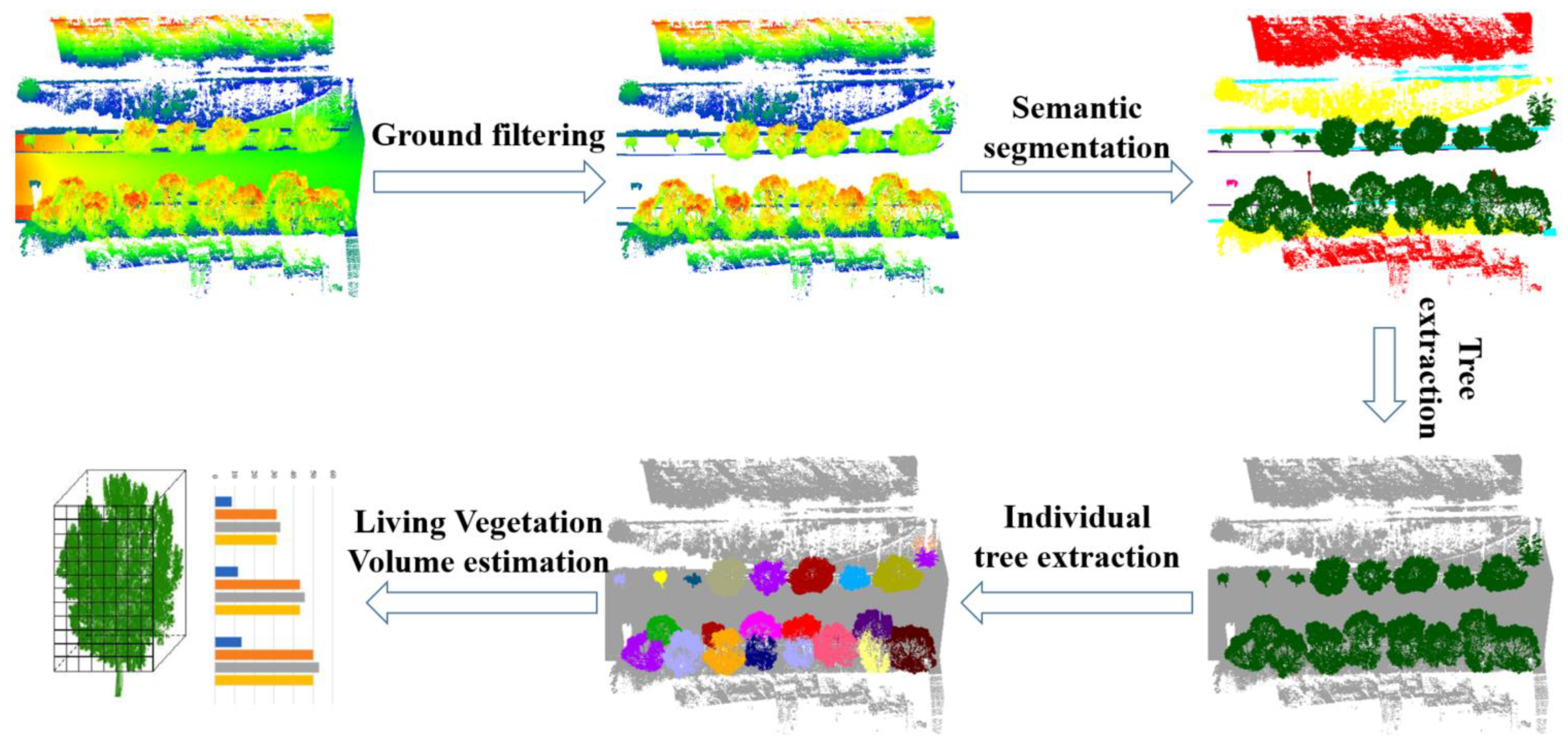
Figure 1. Pipeline of the proposed framework. The tree extraction stage divides the input point cloud into tree and non-tree points. The individual tree separation module takes the tree points as input data and obtains the individual road-side trees.
Remotesensing 15 01992 g001
Figure 2. The overview of the proposed individual tree segmentation method.
Remotesensing 15 01992 g002
Figure 3. The schemes of density-based point convolution.
Remotesensing 15 01992 g003
Figure 4. The illustration of feature fusion module.
Remotesensing 15 01992 g004
Figure 5. The overview of two experimental datasets. These two experimental datasets are colored by elevation of each point.
Remotesensing 15 01992 g005
Figure 6. Example of urban MLS point cloud semantic segmentation on Dataset I. (a) Raw urban MLS point cloud, (b) point cloud semantic segmentation result, dotted in different colors according to the labels, (c) tree point extraction result, where green and gray points represent points from trees and non-tree objects, respectively, (d) two close-up semantic segmentation results at some selected regions.
Remotesensing 15 01992 g006aRemotesensing 15 01992 g006b
Figure 7. Example of urban MLS point cloud semantic segmentation on Dataset II. (a) Raw urban MLS point cloud, (b) point cloud semantic segmentation result, dotted in different colors according to the labels, (c) tree point extraction result, where green and gray points represent points from trees and non-tree objects, respectively, (d) two close-up semantic segmentation results at some selected regions.
Remotesensing 15 01992 g007aRemotesensing 15 01992 g007b
Figure 8. Example of individual tree segmentation on Dataset I. (a) Input tree point cloud, where green and gray points represent points from trees and non-tree objects, respectively, (b) individual tree segmentation result, dotted in different colors, (c) two close-up individual tree segmentation results at some selected regions.
Remotesensing 15 01992 g008aRemotesensing 15 01992 g008b
Figure 9. Example of individual tree segmentation on Dataset II. (a) Input tree point cloud, where green and gray points represent points from trees and non-tree objects, respectively, (b) individual tree segmentation result, dotted in different colors, (c) two close-up individual tree segmentation results at some selected regions.
Remotesensing 15 01992 g009aRemotesensing 15 01992 g009b
Figure 10. Individual tree segmentation results with different methods. Left: individual tree segmentation results; right: the error map of different results. (a) Individual tree segmentation result of watershed-based method [80], (b) individual tree segmentation result of mean shift-based method [81], (c) individual tree segmentation result of SGE_Net [64], (d) individual tree segmentation result of DAE_Net [67], (e) individual tree segmentation result of the proposed method.
Remotesensing 15 01992 g010aRemotesensing 15 01992 g010b
Figure 11. The validation LVV calculation results for two-point cloud datasets. (a) The validation LVV calculation result for Dataset I, (b) The validation LVV calculation result for Dataset II.
Remotesensing 15 01992 g011
Figure 12. Generalization result on ALS point cloud. (a) Raw point cloud, (b) semantic segmentation result, dotted in different colors according to the labels, (c) tree extraction result, where green and gray points represent points from trees and non-tree objects, respectively, (d) individual tree segmentation result, dotted in different colors, (e) close-up for individual tree segmentation.
Remotesensing 15 01992 g012aRemotesensing 15 01992 g012b
Table 1. Semantic segmentation quantitative evaluation (i.e., OA, mIoU and IoU of each class, all values in %) on Dataset I and Dataset II. Best results in bold.
Ref.OAmIoUGroundBuildingTreeLightParterrePedestrainFencePoleCarOthers
Dataset I[39]61.945.360.459.960.862.545.19.67.334.778.034.2
[77]52.337.458.729.950.849.129.110.733.58.681.238.1
[78]52.940.160.267.153.450.813.815.42.960.878.34.8
[41]85.661.788.181.381.582.960.230.226.850.290.750.3
[40]80.259.280.182.165.179.465.270.33.923.491.212.7
[44]82.561.379.277.190.389.545.856.230.166.288.310.3
[20]75.249.672.380.470.279.123.033.678.48.596.130.5
Ours89.163.885.388.987.290.825.659.734.649.895.220.7
Dataset II[39]59.839.655.865.152.737.946.415.310.831.751.029.7
[77]51.037.745.730.239.752.711.58.740.19.635.726.9
[78]52.339.856.770.546.754.712.820.710.945.867.112.5
[41]84.962.685.473.285.778.455.736.922.458.770.160.4
[40]79.850.976.983.770.279.952.144.110.215.766.79.9
[44]80.754.670.870.286.782.723.757.140.851.750.412.4
[20]72.945.053.477.170.470.440.212.110.41.075.740.1
Ours88.864.363.870.888.683.753.430.768.460.145.273.0
Table 2. Instance-level tree segmentation quantitative evaluation on Dataset I and Dataset II. Best results in bold.
Ref.Prec (%)Rec (%)mCov (%)mWCov (%)
Dataset I[80]80.2280.1079.0681.23
[81]82.1481.6782.0183.54
[64]84.5685.2283.9685.24
[67]86.1185.8984.6686.74
Ours90.2789.7586.3988.98
Dataset II[80]82.5482.6980.1281.95
[81]83.9683.4282.4584.02
[64]85.4784.5584.2386.33
[67]88.5387.8685.7486.78
Ours90.8689.2787.2088.56
Table 3. Comparison of LVV calculation results.
This Scheme (m3)Traditional Method (m3)Platform Method (m3) δ 1 (%) δ 2 (%)
Dataset IRoad 19.2310.809.7917.06.1
Road 222.7025.5623.3212.62.7
Road 325.3433.8828.8933.714.0
Average 19.97.8
Dataset IIRoad 413.4116.7715.3725.014.6
Road 532.1136.4834.2913.66.8
Road 639.7646.4042.2916.76.4
Average 16.58.9
Table 4. Instance-level quantitative evaluation on ALS point clouds. Best results in bold.
Prec (%)Rec (%)mCov (%)mWCov (%)
SGE_Net [64]81.2580.5679.5478.24
DAE_Net [67]83.4583.7482.9982.01
Ours88.2387.9486.1285.74
Disclaimer/Publisher’s Note: The statements, opinions and data contained in all publications are solely those of the individual author(s) and contributor(s) and not of MDPI and/or the editor(s). MDPI and/or the editor(s) disclaim responsibility for any injury to people or property resulting from any ideas, methods, instructions or products referred to in the content.