MSFANet: Multiscale Fusion Attention Network for Road Segmentation of Multispectral Remote Sensing Data

Abstract

With the development of deep learning and remote sensing technologies in recent years, many semantic segmentation methods based on convolutional neural networks (CNNs) have been applied to road extraction. However, previous deep learning-based road extraction methods primarily used RGB imagery as an input and did not take advantage of the spectral information contained in hyperspectral imagery. These methods can produce discontinuous outputs caused by objects with similar spectral signatures to roads. In addition, the images obtained from different Earth remote sensing sensors may have different spatial resolutions, enhancing the difficulty of the joint analysis. This work proposes the Multiscale Fusion Attention Network (MSFANet) to overcome these problems. Compared to traditional road extraction frameworks, the proposed MSFANet fuses information from different spectra at multiple scales. In MSFANet, multispectral remote sensing data is used as an additional input to the network, in addition to RGB remote sensing data, to obtain richer spectral information. The Cross-source Feature Fusion Module (CFFM) is used to calibrate and fuse spectral features at different scales, reducing the impact of noise and redundant features from different inputs. The Multiscale Semantic Aggregation Decoder (MSAD) fuses multiscale features and global context information from the upsampling process layer by layer, reducing information loss during the multiscale feature fusion. The proposed MSFANet network was applied to the SpaceNet dataset and self-annotated images from Chongzhou, a representative city in China. Our MSFANet performs better over the baseline HRNet by a large margin of +6.38 IoU and +5.11 F1-score on the SpaceNet dataset, +3.61 IoU and +2.32 F1-score on the self-annotated dataset (Chongzhou dataset). Moreover, the effectiveness of MSFANet was also proven by comparative experiments with other studies.

1. Introduction

Remote sensing technology and data play an essential role in Earth science research. Its research on the automatic extraction of road information from remote sensing images has a wide range of application areas [1,2,3,4], such as autonomous driving [5], traffic management [6] and updating GIS databases [7]. Roads in high-resolution remotely-sensed images usually have the following characteristics: the road is elongated, has two distinct edges, and the texture and grayscale inside the road are often different from those of neighboring areas. Earlier work mainly considered mining road features in images, including radial, geometric, topological, and textural [8,9,10], and morphological features [11,12] and regional growth algorithms [13,14]. Yager et al. [15] implemented road recognition using support vector machines based on edge features, but the accuracy was unsatisfactory. Storvik et al. [16] effectively utilized different spatial resolution images acquired from satellites by integrating multi-resolution image data and Bayesian classification algorithms. The iterative conditional mode (ICM) algorithm gives the final road classification results. However, these well-designed methods are usually target-specific, have low robustness, and are unsuitable for complex environments. The following problems exist in practice: (1) manual feature design requires a lot of time and must be combined with expert knowledge; (2) the effectiveness of these methods depends on several well-designed threshold standards, and traditional methods achieve low accuracy in complex environments, given that threshold settings fluctuate between different scenes.

Road extraction methods using deep learning have received much attention from researchers recently. They have made impressive progress due to their ability to utilize large amounts of data more efficiently than traditional methods. In deep learning methods, the road extraction problem is described as a semantic segmentation problem, where each pixel point of an image is assigned to a class to determine whether it is a road. Many classical semantic segmentation models have been directly applied to the road extraction problem, such as the fully convolutional network (FCN) [17], LinkNet [18], UNet [19], and HRNet [20]. Some researchers have designed unique network structure roads for road features. D-LinkNet expands the receptive field and integrates multi-scale features in the central part while retaining detailed information. In DDU-Net [21], the introduced DCAM uses dilated convolutions for receptive field expansion and multi-scale feature fusion, and uses a spatial channel attention mechanism to realize attention perception. Therefore, more details can be recovered from feature maps and the performance of road extraction in complex environments can be improved. SDUNet [22] builds a structure-preserving model called DULR to explore continuous cues at the spatial level and mitigate information loss, predicting high-resolution road masks using the capabilities of feature encoding based on dense blocks and spatial context information. However, the CNN-based road extraction method is challenging to balance the resolution and perceptual range of the feature map. Moreover, the detailed information contained in the feature map with global dependencies will be continuously decreased when the convolutional layer depth increases. Expanding the receptive field based on dilated convolutions and fusing road features at different scales have proven to be feasible solutions. However, implementing high-precision road extraction algorithms based on deep learning methods is still challenging.

In addition, with the continuous development of remote sensing technology, the volume of remote sensing data has grown significantly. In contrast, a wealth of multi-source and multimodal data has emerged, such as visible imagery (VIS), multispectral imagery (MSI), synthetic aperture radar (SAR), and light detection and ranging (LiDAR). Many researchers are keen to use these images to extract road information and have made progress [23,24,25], but usually, these methods use only single-source data. Different data sources can express different feature information of ground road objects, so fusing different modalities obtained from multiple data sources can achieve better road extraction results. Some approaches have started to explore how road extraction accuracy can benefit from multimodal image information by using complementary features provided by different types of remote sensors [26]. However, there are significant differences in the features expressed between multimodal data generated by different sensors, which may introduce multiple noises when using data from multiple sources. In addition, there are differences in the image resolution of different modal data on the same feature due to sensor limitations.

Inspired by the above discussion, a multiscale Fusion Attention Network (MSFANet) that fuses complementary RGB Pansharpened images and multispectral images is proposed in this paper. Specifically, MSFANet introduces additional multispectral data from which road information is mined. The attention mechanism calibrates different modal data, generates multiscale features, and mines the global contextual information to enhance the semantic representation, providing a general and highly accurate solution for road information extraction. The main contributions of this work are summarized as follows:

(1)

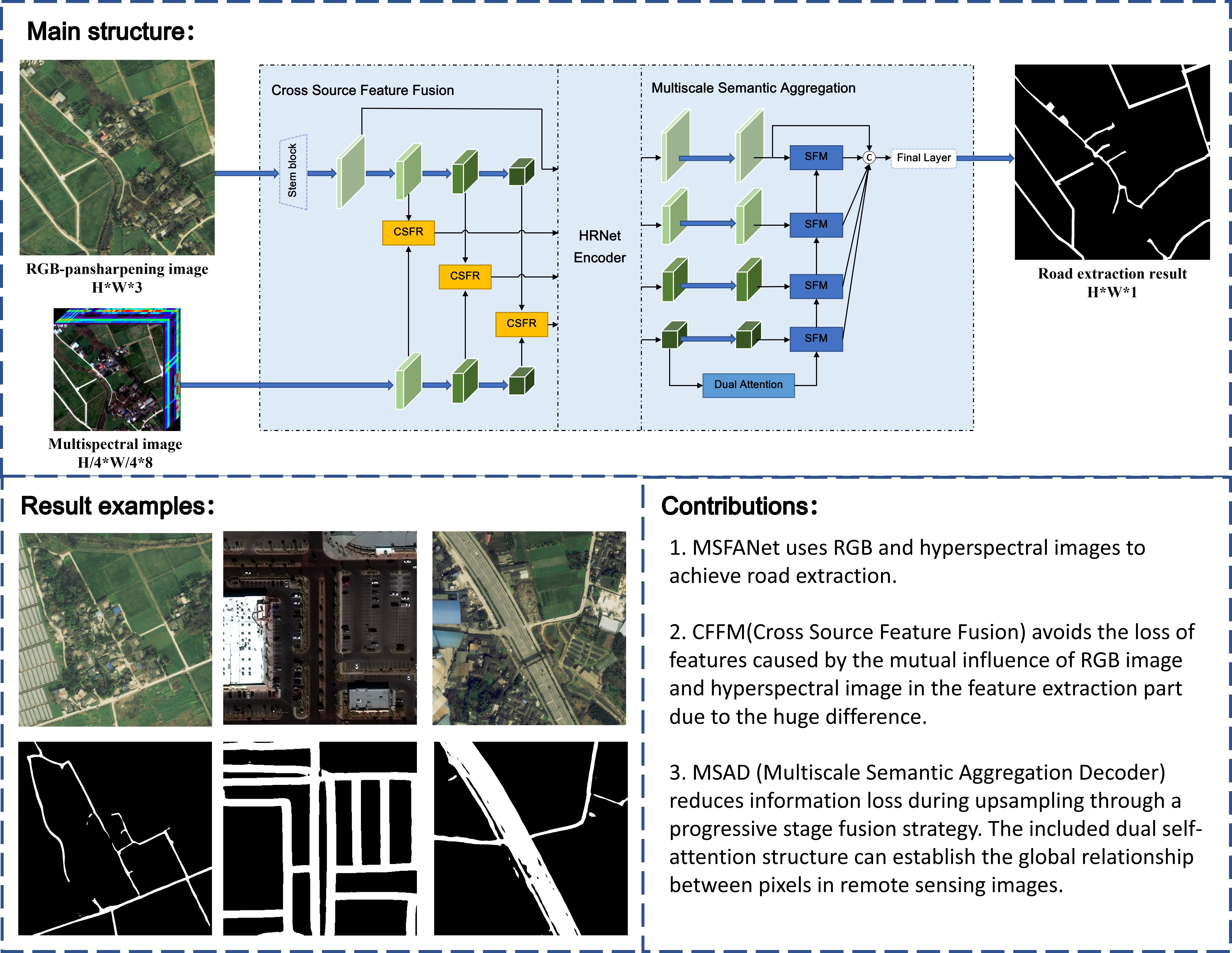
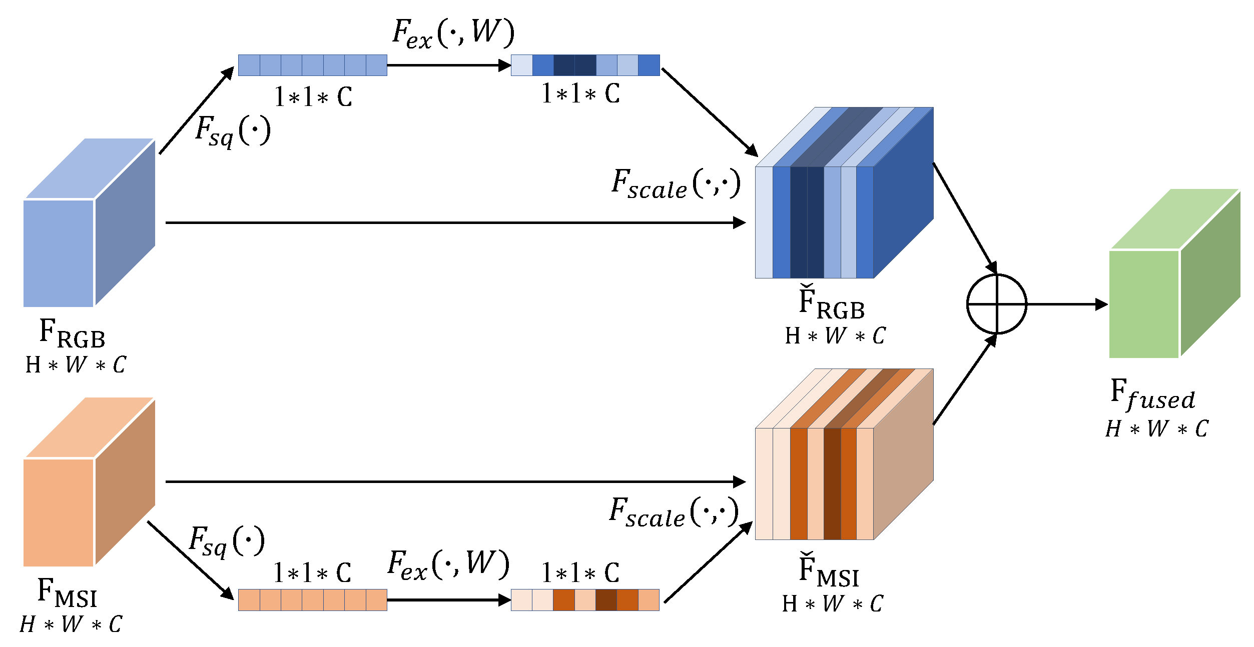
Firstly, we designed the cross-source feature fusion module to generate feature maps at different scales to exploit the semantic representation at different scales and calibrate RGB and multispectral features at different scales by a lightweight attention mechanism to avoid the multiple noises generated by different data;

(2)

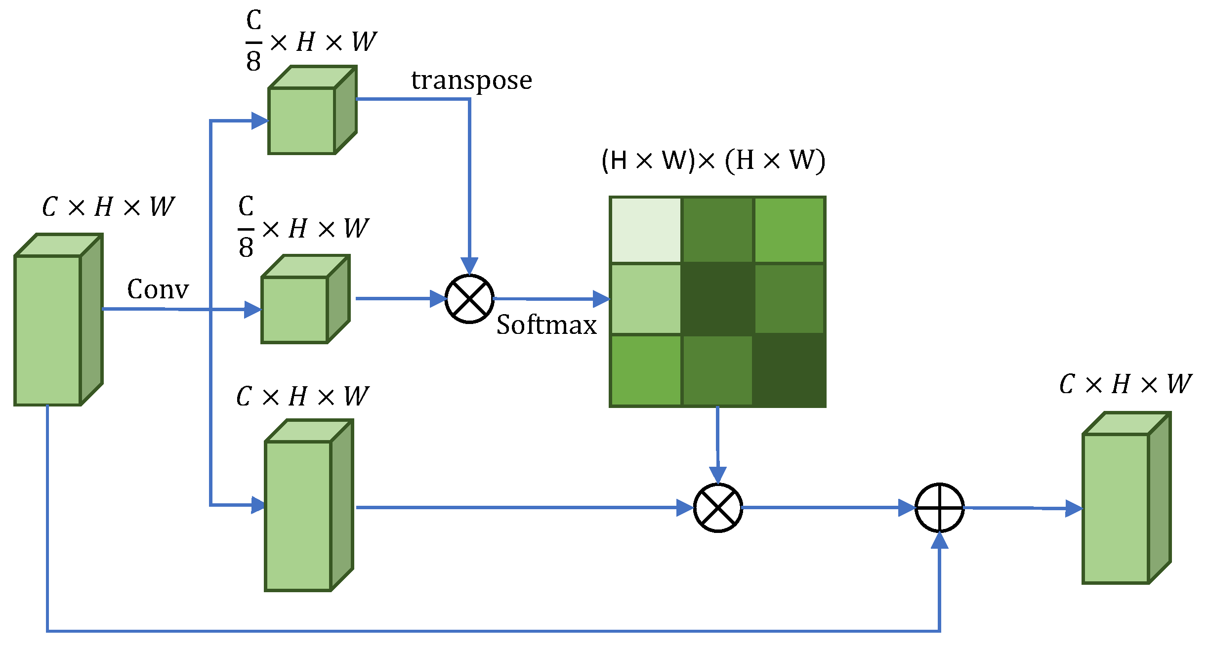
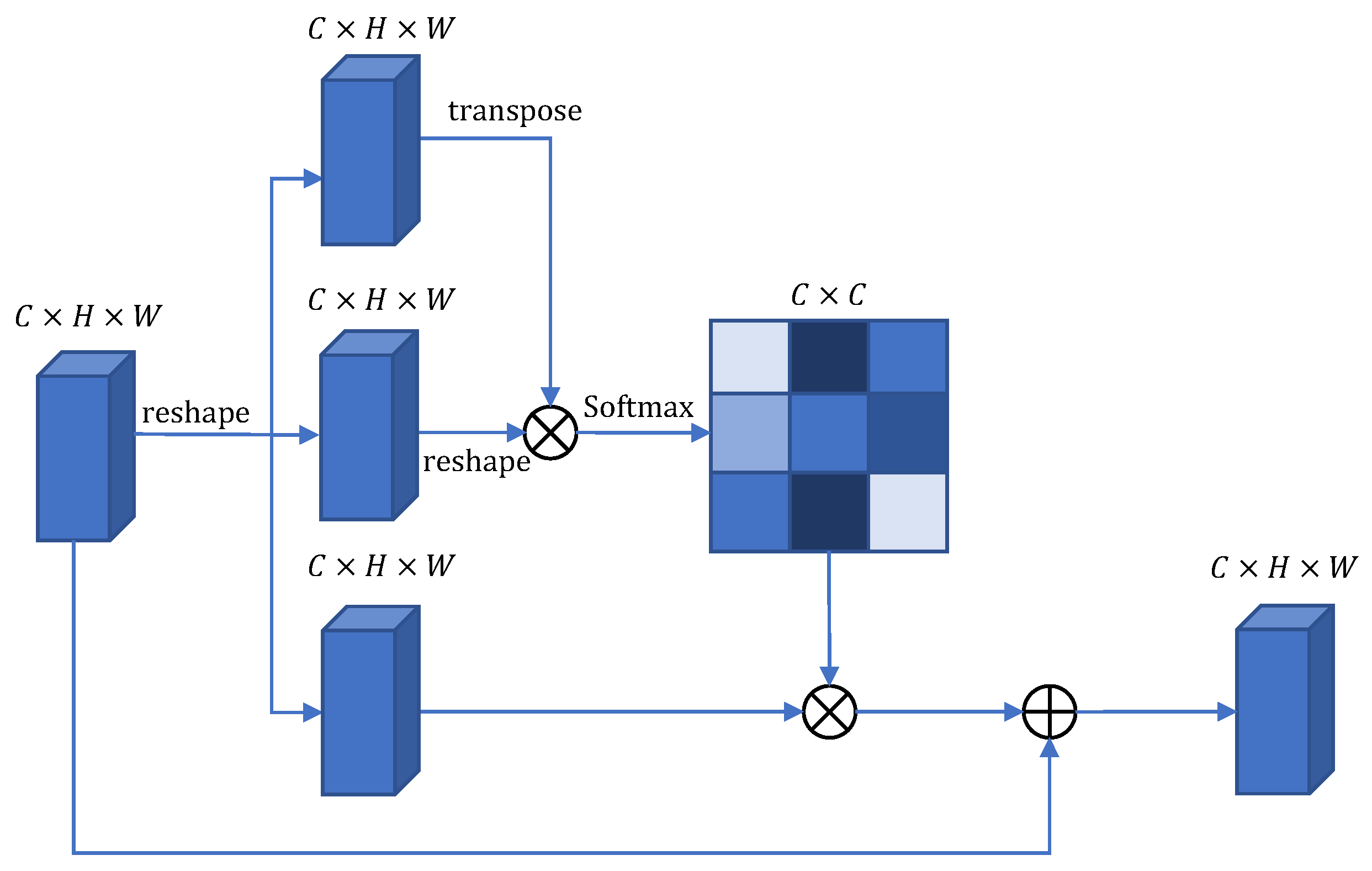
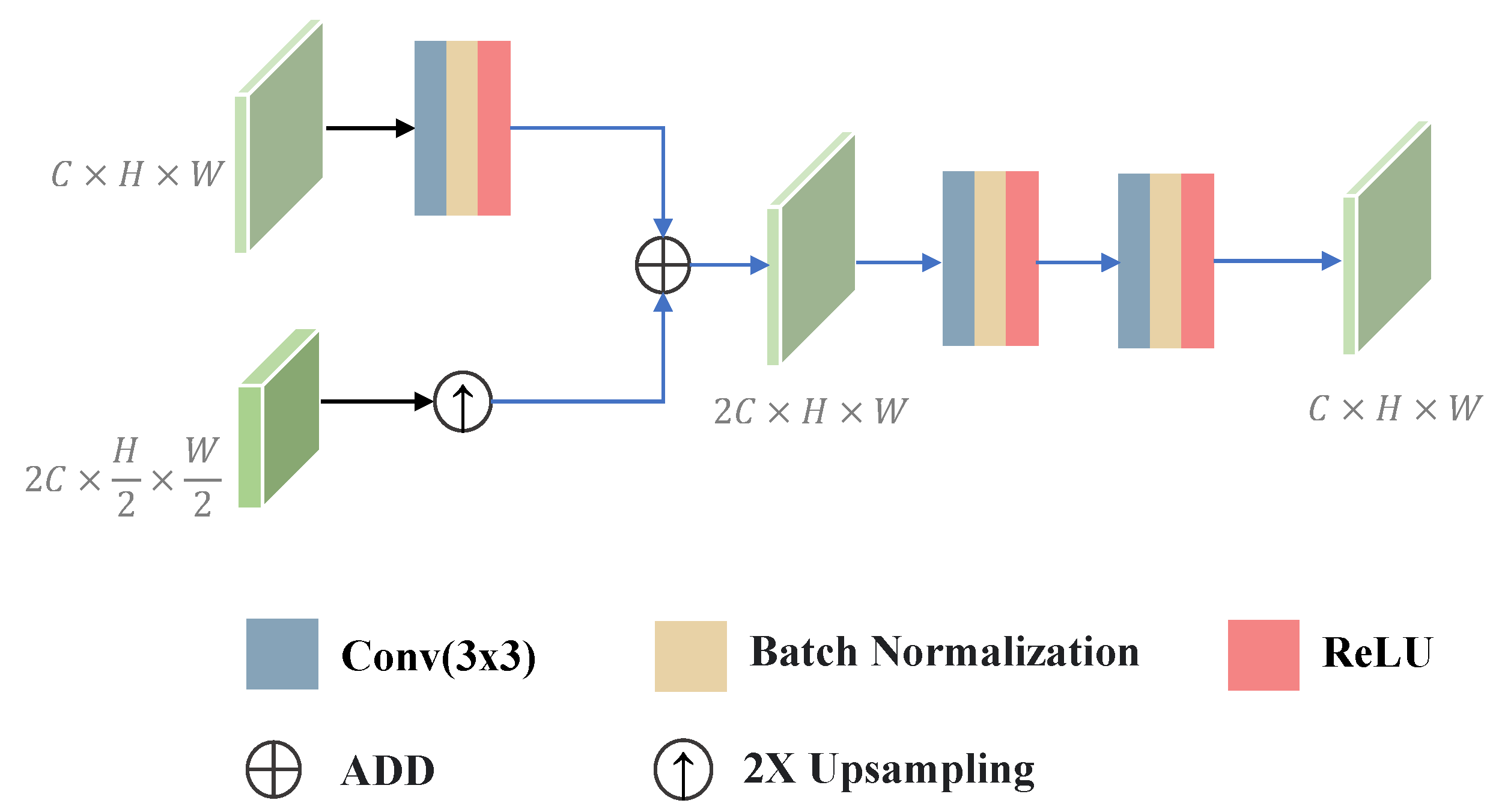
After the HRNet multiscale encoder, we construct a multiscale semantic aggregation decoder to obtain global contextual information in spatial and spectral dimensions using a self-attentive mechanism and fuse and decode feature maps and contextual information at different scales layer by layer to optimize road segmentation results;

(3)

By combining CFFM and MSAD, MSFANet’s performance evaluation implementation on our self-built Chongzhou road dataset and SpaceNet road dataset can show that our proposed model can improve the performance of road extraction and outperform the state-of-the-art models while being competitive in terms of the number of parameters and computational efficiency.

The rest of the paper is organized as follows. Section 2 discusses related work to provide background knowledge for our proposed approach. Section 3 shows the overall structure of our proposed MSFANet and the details of each module. Section 4 shows the dataset, implementation details, and experimental results. The experimental results are analyzed and discussed in Section 5. Finally, Section 6 concludes the study and discusses future work.

2. Related Research

This section introduces some related work in our study, which consists of four parts: Development of Semantic Segmentation Backbone, Segmentation in Remote Sensing Road Extraction, Attention Mechanisms, and Multi-source Data in Remote Sensing Segmentation.

2.1. Development of Semantic Segmentation Backbone

With the development of deep learning and remote sensing image acquisition techniques, novel methods based on convolutional neural networks have received significant attention in road information extraction tasks. When using deep learning methods, the road information extraction problem is described as a semantic segmentation problem, which classifies each pixel on a remotely sensed image as a road or a background. The proposed FCN [17] method provides a basic framework for the semantic segmentation model for the first time: replacing the fully connected layer in traditional CNN with convolutional layers and obtaining pixel-level segmentation results by upsampling feature maps. Based on the FCN framework, some studies have further explored the potential of deep learning methods, e.g., UNet [19] with symmetric encoder-decoder structure and skip connections; PSPNet [27] combining multiscale features with contextual relationships; Deeplabv3+ [28] considering an improved atrous spatial pyramid pooling structure and Xception network. Moreover, HRNetV2 uses multiscale branching to reduce scale feature loss and improve feature representation [20].

2.2. Segmentation in Remote Sensing Road Extraction

Few studies have designed more effective and targeted structures based on road characteristics, considering the complexity of remote-sensing images. For example, D-LinkNet [29] improves the original LinkNet [18] by adding the dilated convolution layer and jump connections to expand the perceptual field while preserving detailed information. Sat2Graph [30] combines segmentation-based and graph-based road extraction methods to map the road extraction problem to detect road edges and vertices, solving the problem of inferring stacked roads such as highway overpasses. HsgNet [31] introduces a Middle Block with the self-attention mechanism in LinkNet to preserve global and second-order spatial information considering the long span, connectivity, and slenderness of roads. In SDUNet [22], a spatial inference module called DULR is introduced to enhance the spatial relationships between different location features using spatial CNNs in four directions to explore road spatial relationships and continuous surfaces. DBRANet [32] proposes a dual-branch network module (DBNM) in the encoding stage to construct more effective features. In the decoding stage, considering the meandering shape and unbalanced distribution of roads in remote sensing images, a Regional Attention Network Module (RANM) is designed to automatically learn the importance of each channel based on regional information. NL-LinkNet [33] proposes an efficient non-local LinkNet with non-local blocks (NLB), which can understand the relationship between global features. This enables each spatial feature to refer to all other contextual information, leading to more accurate road segmentation. In general, existing deep learning road extraction methods mainly have the following improvement strategies: increasing the receptive field of the deep network, mining the spatial relationship of the road from the self-attention structure, and retaining feature information from multi-scale features.

2.3. Attention Mechanisms

Since non-local [34], SENet [35], CCNet [36], and other models introduced attention mechanisms into deep learning networks, many attention-based methods have been proposed and proved to be beneficial to the improvement of semantic segmentation accuracy. DANet [37] constructs a position attention module to learn the correlation of spatial features through the self-attentive mechanism and proposes a channel attention module to model the correlation of channel to integrate local features and global dependencies to improve the feature representation of semantic segmentation. Li et al. [38] combine the attention mechanism and pyramid structure to replace the complex null convolution and argue the importance of global contextual information in semantic segmentation. The attention-based mechanism enables the network to learn global and long-range semantic information, compensating for the information loss generated by the convolutional operation but also bringing a sizeable computational pressure, raising the number of parameters and inference time of the network.

2.4. Multi-Source Data in Remote Sensing Segmentation

In addition, with the increase in the variety of sensors onboard remote sensing satellites, multiple data sources can be obtained for the same area, such as depth images, SAR images, hyperspectral images, LiDAR radar images, and DSM digital surface models. Some research methods [26,39,40,41] are no longer limited to RGB remote sensing image data but start considering other sources and even multi-source data. In MFNet [42], two multi-source fusion modules, IMFintra and IMFinter, are designed to learn the complementary features and cross-modal interdependencies between the two modalities using multi-source VHR aerial images and LiDAR data. Cao et al. [43] developed a cross-modal feature recalibration module (CFR) to aggregate IRRG and DSM data and avoid noise interference between two sources of information. Osmar et al. [44] explored the application of combining multispectral and RGB data for panoramic segmentation on a beach environment, using a Panoptic-FPN architecture with a ResNeXt-101 backbone to improve the segmentation accuracy significantly.

3. Methodology

In this section, we first introduce the basic HRNet structure, then illustrate the framework of our proposed MSFANet, and provide a detailed description of each module in MSFANet.

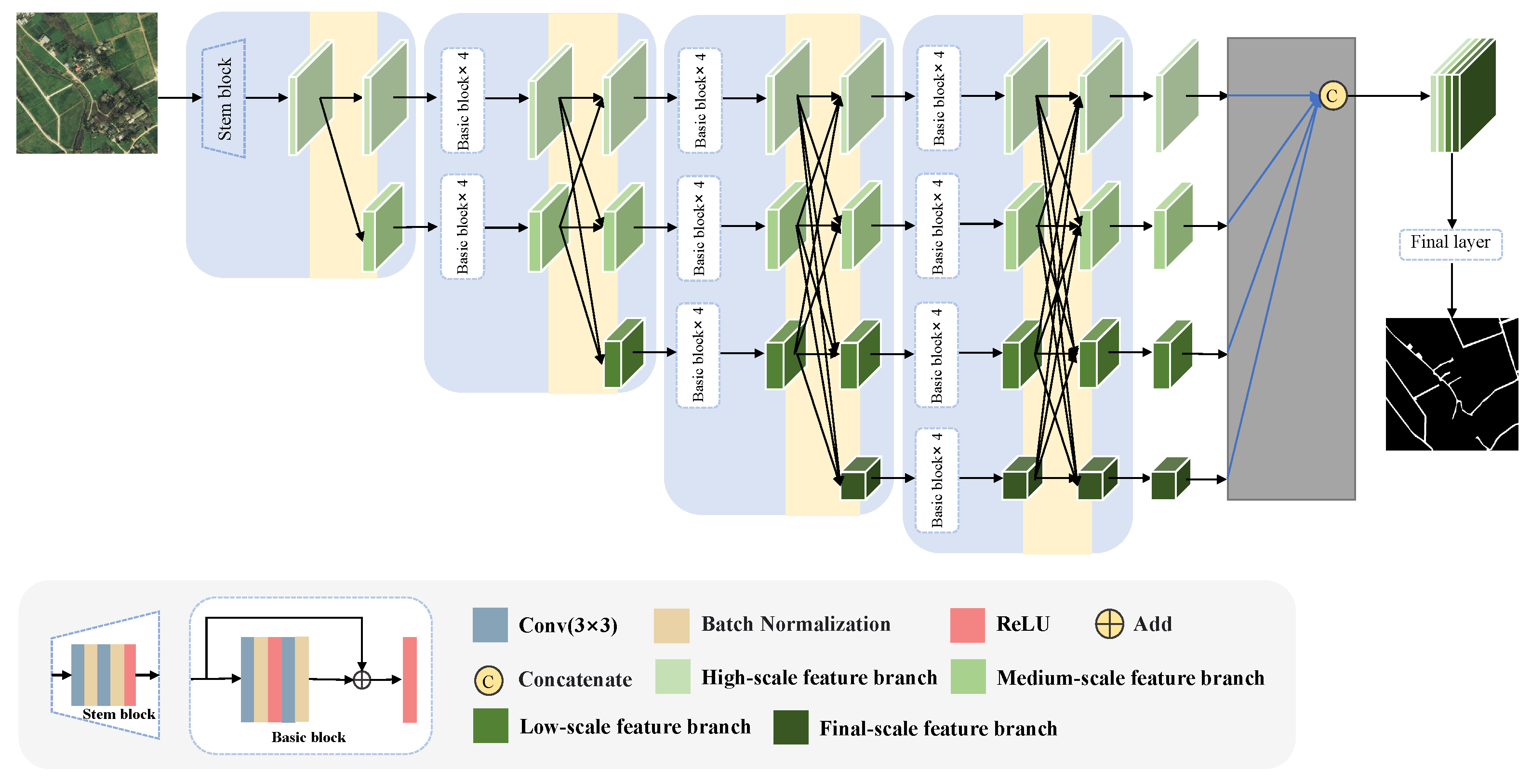
3.1. The Structure of HRNet

As shown in Figure 1, the input of HRNet [20] (size as $H\times W\times C$) is first reduced in size to $\frac{1}{4}$ by Stem Block (two convolutional layers with $3\times 3$ convolutional kernels and two strides), and the number of channels of the feature map is increased to 64. Then, HRNet starts from the high-scale feature branch, keeps the high-resolution features, and downsamples the high-scale feature map to provide the other three parallel-scale feature branches. In addition, the feature maps are fused between the different scale branches, and the fusion method is shown in Figure 2, namely low-scale feature upsampling to a large scale via nearest neighbor interpolation upsampling and 1 × 1 convolution, and relatively high-scale features downsampling to low scale by convolution.

The resolution and number of channels on each branch are $\frac{H}{4}\times \frac{W}{4}\times C$, $\frac{H}{8}\times \frac{W}{8}\times 2C$, $\frac{H}{16}\times \frac{W}{16}\times 4C$, and $\frac{H}{32}\times \frac{W}{32}\times 8C$. In the HRNet paper, the value of the number of channels C can be set by oneself, and it is divided into HRNet_W18 (W18 indicates the width, which means the number of channels is 18), HRNet_W32 and HRNet_W48. To obtain the semantic segmentation output, HRNet upsamples the output of the feature on the four branches to the same size and then mixes them to generate the prediction results. This article uses the HRNet_W32 encoder because it balances operational efficiency and network performance. The multi-branch parallel structure of HRNet considers the acquisition of spatial information. Still, it cannot consider the global contextual information, and the final decoder part loses much multiscale information due to simple scaling.

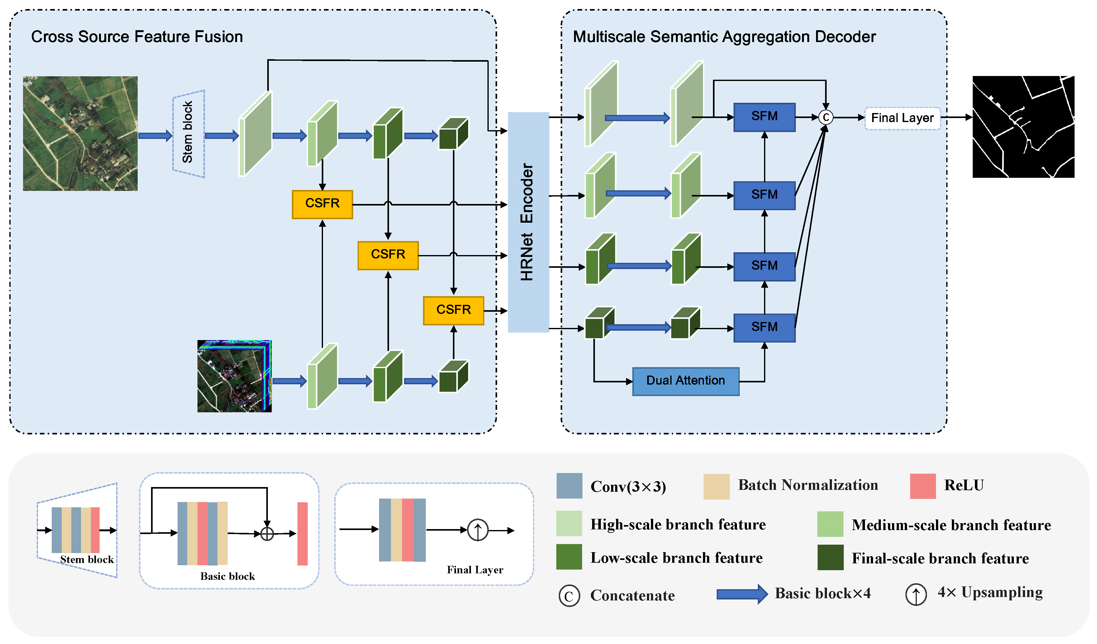
3.2. Architecture of MSFANet

In order to improve the shortcomings of HRNet and introduce a multi-source data input, we designed the structure of MSFANet. Figure 3 shows the network structure of MSFANet, which mainly consists of cross-source feature fusion, HRNet encoder, and multiscale semantic aggregation. Firstly, the multiple-scale feature maps are obtained on RGB and hyperspectral images by stacking convolutional layers separately. The Cross-source Feature Recalibration Module (CFRM) achieves feature recalibration and fusion at each scale. Second, HRNet is a feature encoder to obtain semantic information at four scales. However, here HRNet does not directly derive segmentation results but aims to obtain semantic features of different branches. Next, multiscale semantic aggregation is used to reconstruct the high-resolution features, expand the perceptual field, and obtain the contextual information using the dual-attention structure. Then, progressively fuse the four scale branches using the low-to-high structure to obtain the segmentation results.

3.3. Cross-Source Feature Fusion Module

When we use RGB images and hyperspectral images as network inputs, the apparent problem is the difference in the resolution of the two images. In addition, the additional data, although providing more information, also introduces more noise leading to bias in extracting features. Introducing multiple data sources focuses on how to solve these two problems. The Cross-source Feature Fusion Module (CFFM) solves the problem in two ways: (1) by generating feature maps to exploit the semantic representation at different scales, and (2) by fusing multi-source data (RGB and multispectral images) using additional multispectral data to complement the features to enhance the feature representation. The structure of the CFFM is shown on the right of Figure 3.

For this purpose, we first extract feature maps at different scales from RGB and hyperspectral images using the convolution module, respectively. Then, we fuse the RGB and hyperspectral feature map pairs at the same scale by Cross-source Feature Recalibration Module (CFRM), where the attention mechanism is used to calibrate the two feature maps. As shown in Figure 4, we generate two feature vectors from the RGB and hyperspectral feature maps with the same channels as the input feature maps. The feature vectors are used to learn the dependency on each channel and adjust the feature maps according to the dependency. The parameters of the feature vectors can be continuously updated with the training process to filter the noise and highlight the key information. As shown on the left side of Figure 3, the fusion of features at three scales is achieved, providing the calibrated fused feature information at different resolutions from low to high. The fused features are used as input to the HRNet encoder. The method of generating feature vectors is shown in Figure 4, which consists of two main parts: Squeeze and Excitation. Squeeze($F_{sq}$) compresses the original feature map to the dimension of $1\times C\times C$:

$$z_c=F_{sq}\left(F_c\right)=\frac{1}{W\times H}\sum _{i=1}^W\sum _{j=1}^H{F}_c(i,j)$$

(1)

where $z_c$ is the compressed vector, c represents the cth element of z, and W and H are the width and height of the original feature map.

Excitation ($F_{ex}$) contains two fully connected layers with two nonlinear activation functions, and the feature vector learns the required weight information from Excitation, whose formula is given. The final fused feature information is the sum of the RGB and hyperspectral recalibration feature maps.

$$S=F_{ex}(z,W)=\sigma \left(g(z,W)\right)=\sigma (W_2,\delta (W_1,z))$$

(2)

$$F_{fused}=S_{RGB}·F_{RGB}+S_{MSI}·F_{MSI}$$

(3)

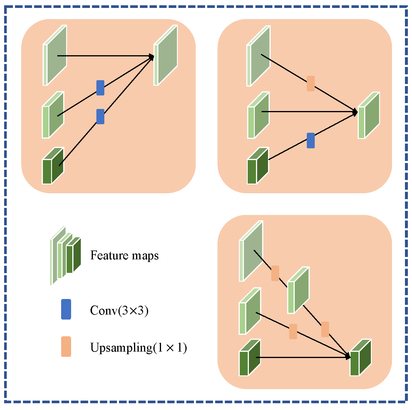
3.4. Multiscale Semantic Aggregation Decoder

When HRNet performs semantic segmentation, one obvious problem is that in the final encoder part, it only upsamples four different scales of feature maps to the highest resolution and then performs the Concat operation. It then obtains the segmentation results in a convolutional layer. The disadvantage is obvious: the decoding process needs to be simplified, but we must take full advantage of the information in the different scale branches. In addition, the direct up-sampling to the highest resolution also results in much information loss. The lowest branch feature map requires an 8× up-sampling, which is an unacceptable loss.

We propose a Multiscale Semantic Aggregation Decoder (MSAD) to address this problem. The structure of MSAD can be seen on the right side of Figure 3. First, we use the global context-aware module to construct the global information of the network in spatial and channel dimensions from the feature maps of the lowest-resolution branches. The structure of the global context-aware module contains a convolutional branch and a dual self-attention branch, which is inspired by DANet [37]. It consists of a position self-attention module (PAM) and a channel self-attention module (CAM), which improves the focus on the road target and enhances the network’s capability. Introducing PAM and CAM allows us to capture spatial global dependence information and the importance of different channel dimensions. In the dual attention branch, the feature map output by the HRNet encoder is subjected to PAM and CAM computations to obtain the spatial dependency between any two positions in the feature map and the channel dependency between any two channels. Finally, the outputs of the two attention modules are fused to further improve the feature representation. The formula for the dual attention module is as follows:

$$F_{DA}=F_{PAM}+F_{CAM}=PAM\left(F_{in}\right)+CAM\left(F_{in}\right)$$

(4)

where $F_{DA}$ is the output of the dual self-attention module, $F_{PAM}$ and $F_{CAM}$ are the feature maps computed by PAM and CAM, respectively, the $PAM\left(\right)$ and $CAM\left(\right)$ representing the position and channel attention operations, $F_{in}$ is the input of the dual self-attention module.

For later description, we agree on the following notation: C, H, and W denote the channel, height, and width of the feature map for computing attention. Q, K, and V refer to the attention mechanism’s query, key, and value features. The structure of the PAM is shown in Figure 5. In the PAM, the input of $C\times H\times W$ generates three feature maps. After two of them are convolved, the number of channels becomes $\frac{C}{8}\times H\times W$, which is used as the Q and K in the attention mechanism to compute the spatial attention probability map of shape $(H\times W)\times (H\times W)$. PAM uses a spatial attention map to select aggregating contexts. PAM also has a global contextual view. Semantic features improve intra-class compactness and semantic consistency. Subsequently, reshape the attention graph and obtain the final prediction graph. The structure of the PAM calculation is shown in Equations (5) and (6), where $At{t}_{PAM}$ is the attention probability map obtained by PAM, $Input$ is the input to the PAM module, and $F_{PAM}$ is the result of the feature map calculated by PAM. $.reshape\left(\right)$ is a reshape operation. The subscripts represent the dimensions of the corresponding feature maps.

$$At{t}_{PAM}=softmax(Q_{(HW\times C)}·K_{(C\times HW)})$$

(5)

$$F_{PAM}=(V_{(C\times HW)}·At{t}_{PAM}).reshape(C\times H\times W)+Inpu{t}_{(C\times H\times W)}$$

(6)

The structure of CAM is shown in Figure 6 and is similar to PAM. However, the computed feature probability map is $C\times C$, which aims to focus on the connection between different feature channels. CAM is similar in structure to PAM, the first difference being that there are fewer channels, so there is no need to change the shape of the feature map using convolution to reduce the number of operations. The other difference is that the shape of the generated attention weight map is changed, as CAM focuses on the connections between the different channels of the features. In the network structure, CAM establishes the influence relationship between the features of different channels by swapping the position of the dot product of the location attention module and the shape of the generated attention weight map is (C × C). Because of the variation in the feature probability map, CAM does not need to reduce the dimensionality of Q and K using the convolution operation to reduce the computation. The structure of CAM calculation is shown in Equations (7) and (8). where $At{t}_{CAM}$ is the attention probability map obtained by CAM, $Input$ is the input to the CAM module, and $F_{CAM}$ is the result of the feature map calculated by CAM. $.reshape\left(\right)$ is a reshape operation. The subscripts represent the dimensions of the corresponding feature maps.

$$At{t}_{CAM}=softmax(Q_{(C\times HW)}·K_{(HW\times C)})$$

(7)

$$F_{CAM}=(At{t}_{CAM}·V_{(C\times HW)}).reshape(C\times H\times W)+Inpu{t}_{(C\times H\times W)}$$

(8)

After the global context-aware module, the obtained feature maps are progressively fused with different branch feature maps by the Smooth Fusion Module (SFM). The structure of the Smooth Fusion Module is shown in Figure 7. The purpose of the SFM is to continuously connect multiscale information from different branches to enhance the feature representation of the network by gently increasing the resolution of the feature map without losing too much information due to aggressive upsampling operations. Finally, we concatenate all the feature maps after SFM to enhance the global information representation of each feature map and thoroughly learn the feature information at different scales. After that, we obtain the road segmentation results from the final feature maps output by the last layer of convolution.

4. Experiments

We validate the effectiveness of MSFANet by conducting comprehensive experiments on our Chongzhou road dataset and the publicly available SpaceNet road dataset [45]. We compare the proposed method with other road extraction methods. In addition, we use HRNet and our method for ablation experiments. In addition to the experiments of the proposed method, we compared seven deep learning methods: LinkNet [18], DLinkNet [29], HRNet [20], CCNet [36], DANet [37], DBRANet [32] and NLLinkNet [33]. D-LinkNet, DBRANet and NLLinkNet are models focusing on road extraction from remote sensing images. CCNet and DANet are characterized by the use of self-attention structures. HRNet is the baseline method of our proposed method. All comparison networks follow the architecture in the original papers, i.e., we did not change their structure. We conducted two separate experiments on Chongzhou and SpaceNet datasets. The first experiment was conducted on the Chongzhou dataset, and the second experiment was conducted on the SpaceNet dataset. In order to ensure fairness, no pre-trained weights and no additional data were used in the training process.

4.1. Dataset Descriptions

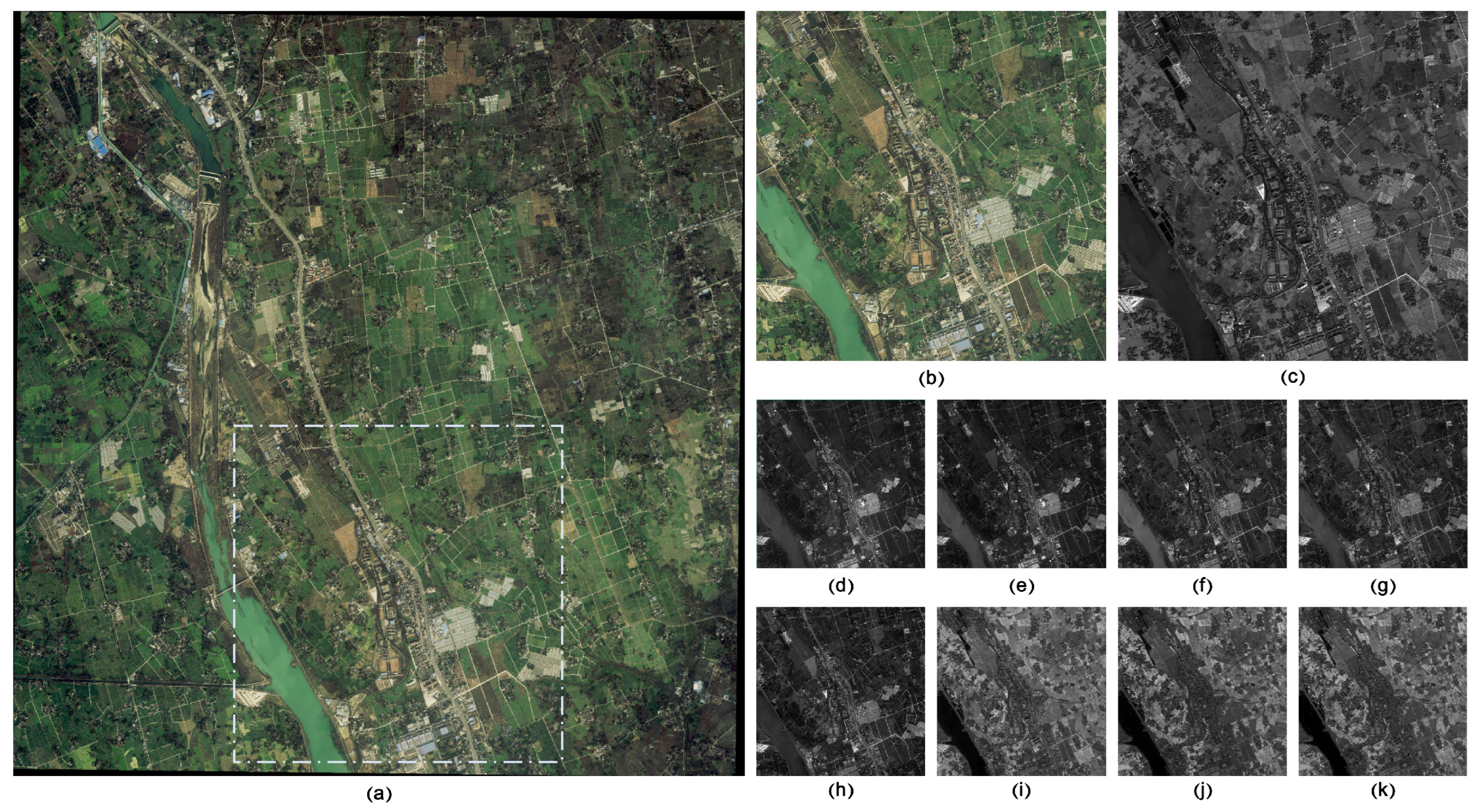
4.1.1. Chongzhou Road Dataset

The remote sensing image source for our self-constructed Chongzhou dataset is from the Worldview3 satellite taken on 13 May 2018, in the Chongzhou region of Sichuan Province, China. The high-resolution WV-3 image contains eight (1.2 m) spectral bands and one panchromatic band (0.3 m), and each band and the corresponding wavelengths are shown in

Table 1. Worldview3 sensor bands with corresponding wavelengths.

Band Name	Spectral Band
Panchromatic Band	450–800 nm
Coastal Blue	400–450 nm
Blue	450–510 nm
Green	510–580 nm
Yellow	585–625 nm
Red	630–690 nm
Red edge	705–745 nm
Near-IR1	770–895 nm
Near-IR2	860–1040 nm

. We apply the panchromatic sharpening method to obtain high-resolution RGB-pansharpening images, combining the spatial information of the panchromatic band and the spectral information of the multispectral band. Therefore, this dataset contains two source images, the three-band RGB-pansharpening image and the eight-band hyperspectral image. For convenience, the three-band RGB-pansharpening image will be directly referred to as the RGB image in subsequent papers.

The three-band RGB image size is 22,904 × 23,592, corresponding to the eight-band hyperspectral data size of 5726 × 5898. We crop the image to extend the dataset by using a 1024 × 1024 cropping area on the RGB data, and to keep the cropped areas still corresponding to each other, the cropping area on the hyperspectral data is 256 × 256. The cropped data are divided into training, validation, and test sets. We performed data enhancement on the training set, including rotation and flip operations. Finally, we obtained a training set containing 4140 training images, 92 validation images, and 180 test images. An example of imagery from the Chongzhou dataset can be seen in Figure 8.

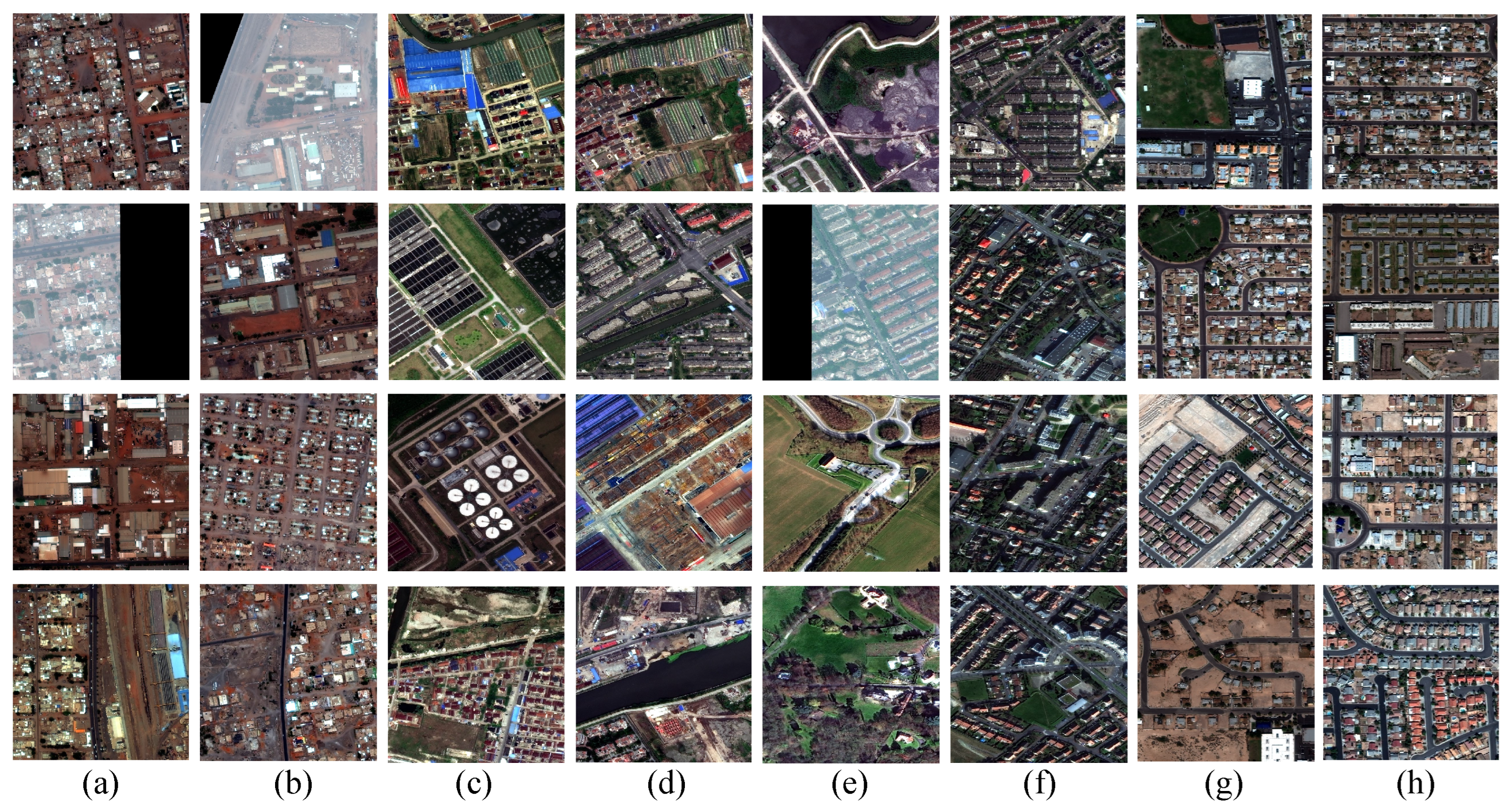
4.1.2. Spacenet Road Dataset

The Spacenet dataset [45] provides WorldView3 satellite data for four regions, Las Vegas, Paris, Shanghai, and Khartoum with three-band RGB-pansharpening images with a ground resolution of 30 cm/pixel and a pixel resolution of 1300 × 1300 per image and eight-band hyperspectral images with a ground resolution of 120cm/pixel and a pixel resolution of 325 × 325 per image. Since the Spacenet dataset provides annotations of road centerlines, we need to pre-process the dataset to apply it to semantic segmentation. First, we convert the 11-bit images of the original dataset to eight-bit images, create a road mask based on the road centerlines, and obtain a new dataset. To increase the train set and facilitate training, we create four 512 × 512 cropping regions for each RGB-pansharpening image and four 128 × 128 cropping regions on the hyperspectral images in the corresponding regions. Then, we divided the dataset into training, test, and validation sets according to the Batra et al. [46] division for training. Finally, we obtained about 18,000 training images, 3500 test images and about 1,200 validation images. Some images of different regions in the SpaceNet dataset are shown in Figure 9.

4.2. Implementation Details and Metrics

Table 2. Experiment settings.

System	Ubuntu 18.04.6
HPC Resource	NVIDIA GeForce RTX 3090 Ti
DL Framework	Pytorch V1.11.0
Compiler	Python V3.9.12
Optimizer	AdamW
Loss Function	CEloss
Learning Rate	0.001
LR Policy	PolyLR
Batch Size	4 (ChongZhou), 8 (SpaceNet)

shows the experimental setup on two training sets, all models were trained and tested on an NVIDIA 3090TI 24GB graphics card, and we implemented the proposed models and other network architectures in the Pytorch framework. We use the poly learning rate policy to improve the efficiency of training, which is represented as follows:

$$lr=initial\_lr{(1-\frac{iter}{max\_iter})}^{power}$$

(9)

$lr$ refers to the learning rate. Furthermore, $initial\_lr$ is the initial learning rate set as 0.001 at training time, $iter$ is calculated based on the current epoch, $max\_iter$ is the product of the training epoch, and the number of training set images. $Power$ is set to 0.9 as a hyperparameter.

We use the cross-entropy loss as the loss function, defined as Equation (10). Where N is the total number of classes, y and y’ are the semantic labels and the network’s predictions, respectively.

$$L_{ce}=-\frac{1}{N}\sum _{i=0}^N(y{log}_{}{y}^{{}^{\prime }}+(1-y){log}_{}(1-y^{{}^{\prime }}))$$

(10)

Since roads occupy only a tiny part of the image in the road segmentation task and most of it is background, which leads to severe class imbalance, it is more appropriate to use F1 score, mIoU, and road IoU metrics to judge the network effect. During the testing phase, we evaluate the network performance using five metrics: Precision, Recall, F1_score, IoU, and mIoU. The formula is shown below:

$$Precision=\frac{TP}{TP+FP},Recall=\frac{TP}{TP+FN}$$

(11)

$$F1\_score=\frac{2\times precision\times recall}{precision+recall}$$

(12)

$$IoU=\frac{TP}{TP+FP+FN}$$

(13)

$$mIoU=\frac{1}{k+1}\sum _{i=0}^k\frac{TP}{TP+FP+FN}$$

(14)

P, N, TP, FP, and FN represent the positive, negative, true positive, false positive, and false negative pixels in the prediction map, respectively.

4.3. Results and Analysis

Table 3. Evaluation results obtained by IoU (%), mIoU (%), F1-score (%), precision (%) and recall (%) on the Chongzhou and SpaceNet datasets. Best results are shown in bold.

Method	IoU	mIoU	Recall	Precision	F1
ChongZhou Dataset
LinkNet [18]	72.87	85.99	85.60	83.00	84.28
DLinkNet [29]	76.44	87.85	89.30	84.20	86.68
HRNet [20]	75.16	87.19	89.10	82.80	85.84
CCNet [36]	77.48	88.39	90.50	84.40	87.34
DANet [37]	73.02	86.07	85.60	83.30	84.43
DBRANet [32]	78.17	88.74	90.50	85.20	87.77
NLLinkNet [33]	76.12	87.68	89.30	83.80	86.46
Ours	78.77	89.05	90.20	86.20	88.16
SpaceNet Dataset
LinkNet	58.13	76.55	69.70	77.70	73.48
DLinkNet	59.79	77.44	72.80	77.00	74.84
HRNet	55.07	74.88	65.30	77.80	71.00
CCNet	59.27	77.18	71.40	77.80	74.46
DANet	60.16	77.66	72.90	77.50	75.13
DBRANet	59.66	76.83	88.20	71.00	73.97
NLLinkNet	58.77	76.87	76.70	71.50	74.01
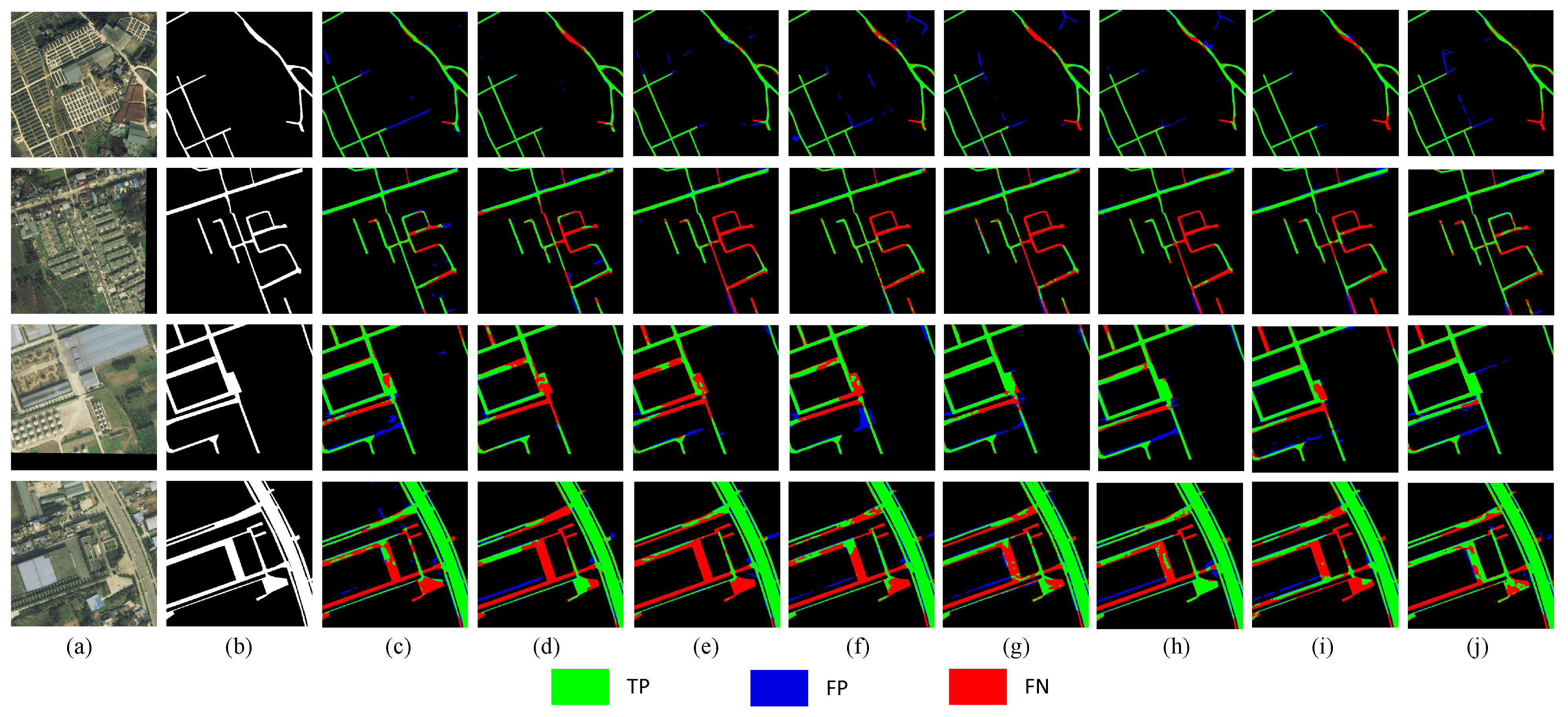
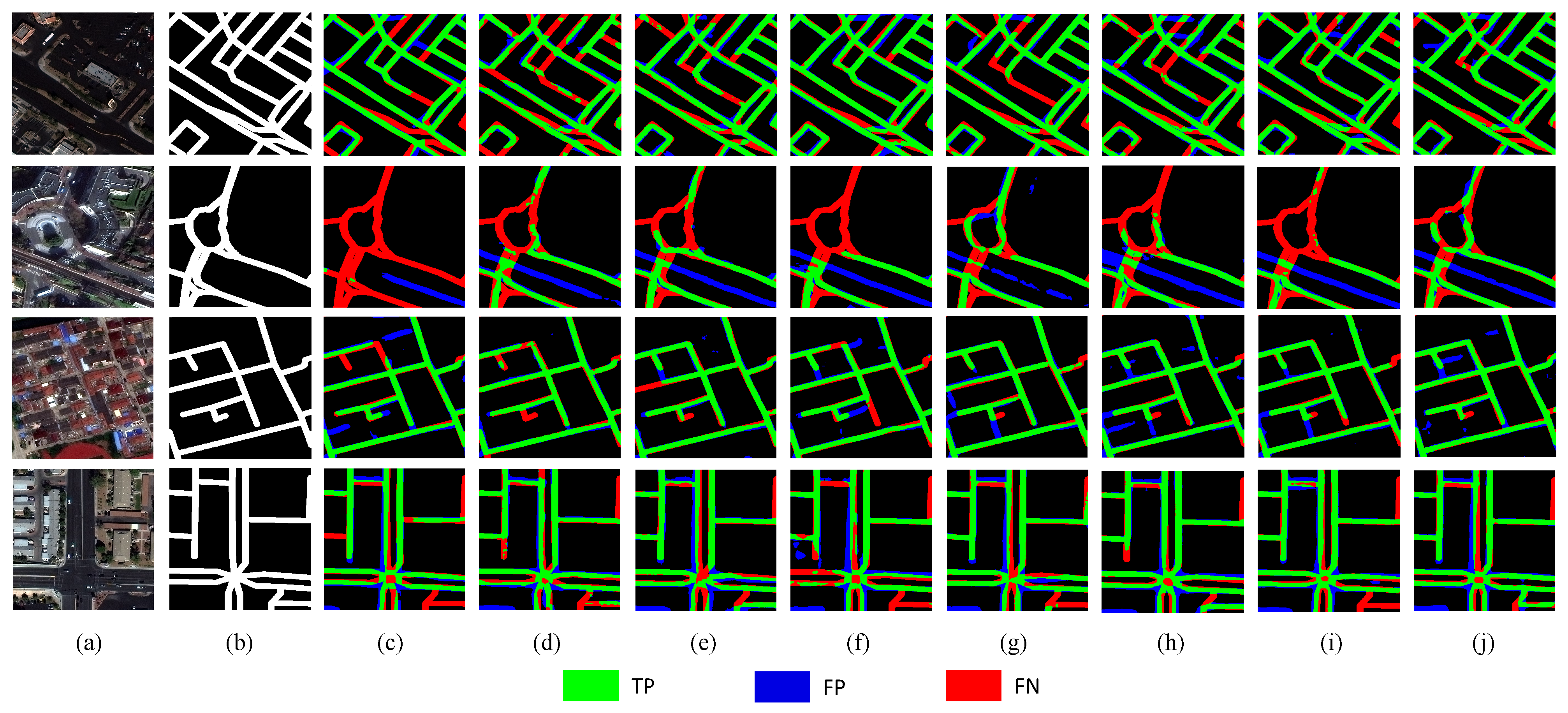
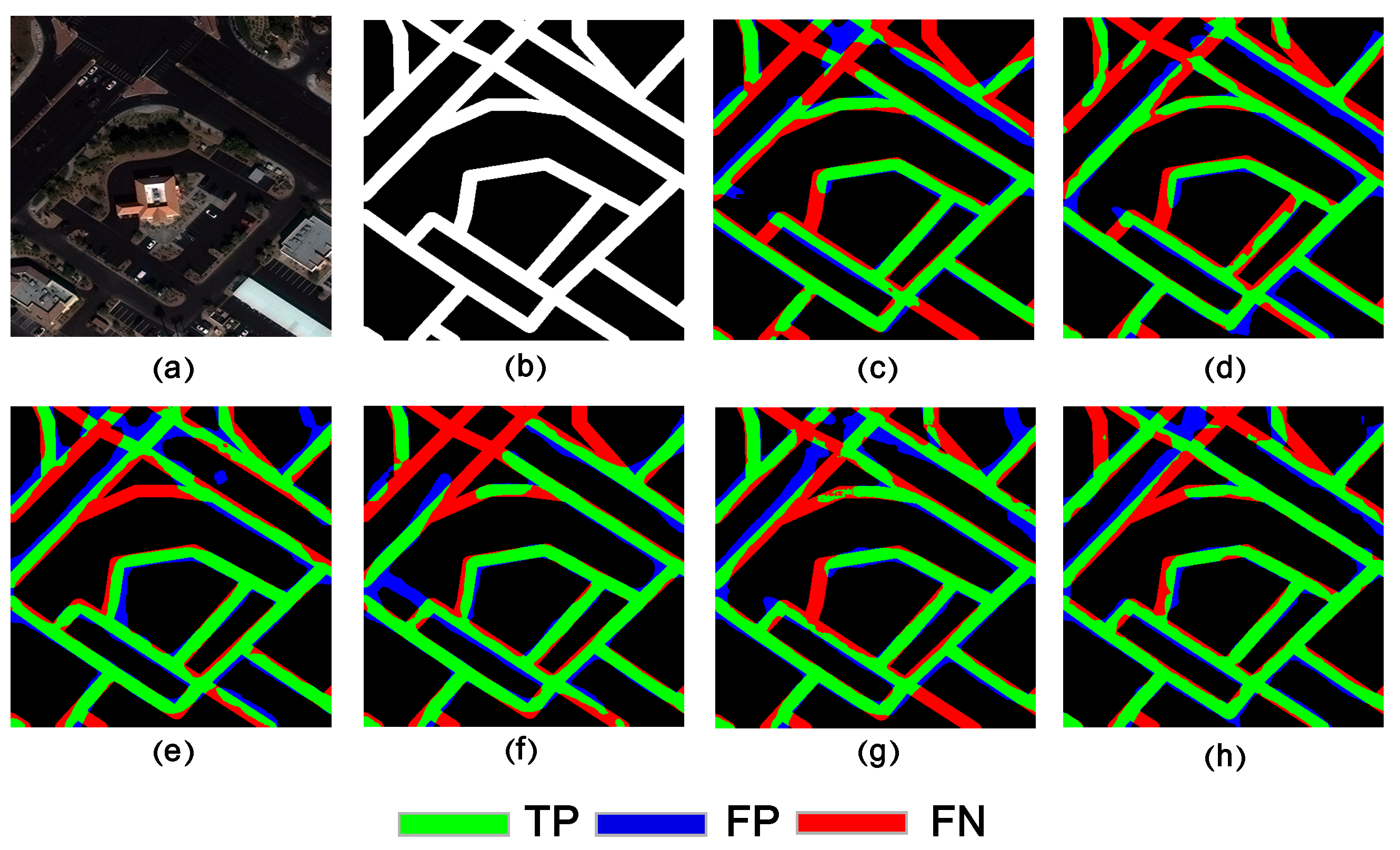
Ours	61.45	78.38	74.50	77.80	76.11

presents the quantitative experimental results of the six evaluation models on the Chongzhou data set. In addition to our proposed method, we also tested and compared it with the other seven methods: LinkNet [18], D-LinkNet [29], HRNet [20], CCNet [36], DANet [37], DBRANet [32], and NL-LinkNet [33]. Table 2 shows that our proposed method outperforms LinkNet, D-LinkNet, HRNet, CCNet, DANet, DBRANet, and NL-LinkNet in terms of F1 score by 3.88%, 1.48%, 2.32%, 0.82%, 3.73%, 0.39%, and 1.7%. In IoU, it is better than LinkNet, D-LinkNet, HRNet, CCNet, DANet, DBRANet, and NL-LinkNet, with 5.9%, 2.33%, 3.61%, 1.29%, 5.75%, 0.6% and 2.65%. In terms of recall, CCNet is slightly higher than our method. However, in terms of accuracy, IoU, mIoU and F1 score, our method performs better than the other methods.

Figure 10 shows the segmentation results of each network based on each Chongzhou dataset. The segmentation results are divided into three categories after comparing with the labels:

(1)

TP is the result of correct segmentation, colored green.

(2)

FP is the result of labeled background but identified as a road during segmentation, colored blue.

(3)

FN is the result of the road not being identified during segmentation, colored red.

Figure 10 shows that MSFANet performs well for road extraction in multiple complex scenes with high robustness. The figure shows that most road areas can be extracted correctly by these six methods, but there are still some segmentation errors. The analysis of these errors also shows the excellence of MSFANet compared with other methods.

From the first rows, based on MSFANet, we can benefit from the extraction of diverse information from different spectra, improve the connectivity and smoothness of the road extraction in the occluded region, and suppress the generation of some erroneous extractions. The second row shows the results of different methods for segmentation when the road is occluded by shadows and other dense features (complex background scenes). It can be seen that the difficulty of recognition in the heavily occluded area increases significantly, and the three methods, HRNet, CCNet, and DANet, can hardly recognize the specific area. Our proposed method is more effective in extracting this part of the road. In the third and fourth rows, examples are shown to evaluate the effectiveness of each method when the road colors (RGB, visual) are similar or when the semantic information around the road is very similar, generating interference. All six networks produce some degree of incorrect segmentation results in these regions due to the interference of similar information. However, MSFANet is more effective in suppressing some false recognition and optimizing the segmentation fineness in some regions.

In addition to the experiments on our self-built Chongzhou dataset to illustrate the model’s generalization, we also conducted tests on the publicly available SpaceNet. The quantitative results of the eight methods on the SpaceNet dataset are also shown in Table 3. In terms of IoU metrics, MSFANet outperforms HRNet, LinkNet, D-LinkNet, CCNet, DANet, DBRANet and NL-LinkNet by 6.38%, 3.32%, 1.66%, 2.18%, 1.29%, 1.79%, and 2.68%, respectively. Regarding F1 scores, MSFANet is higher than HRNet, LinkNet, D-LinkNet, CCNet, and DANet by 5.11%, 2.63%, 1.27%, 1.65%, 0.98%, 2.14%, and 2.1%, respectively. The increase in metrics proves the superiority of MSFANet on the SpaceNet dataset.

Recall indicates the percentage of correctly predicted roads. The recall value of MSFANet on the SpaceNet dataset is at the same level as other methods, proving the MSFANet network’s segmentation ability. As for the accuracy rate, MSFANet significantly improved compared to other methods. The accuracy rate illustrates the correctness of all the road prediction results, showing that MSFANet can suppress the error of identifying the background as a road on the SpaceNet dataset.

From Figure 11, MSFANet segmentation in SpaceNet has an advantage in suppressing errors. In addition, it can be seen from the second and third rows that the segmentation results obtained by MSFANet identify some regions that are difficult to identify by other networks. Compared with other models, our results show better continuity on the road, as in the first and fourth rows. In the fourth row, the road feature in the lower right corner is difficult to recognize on the RGB image, which makes the other reference models produce incorrect segmentation. In contrast, MSFANet can extract road results better due to the introduction of multispectral data and global contextual information.

Compared with other networks, MSFANet obtains better segmentation results in many cases, even in complex scenes. On the one hand, introducing multispectral data allows MSFANet to optimize the extraction of some occlusion and semantic information similar to regions. On the other hand, the fusion of multiscale features and the consideration of contextual information refine the extraction results. Overall, MSFANet extracts complete and connected roads than other methods. It also achieves better results for narrow roads and occlusion problems where the roads are close to the background features.

4.4. Ablation Study

To demonstrate the effectiveness of introducing multispectral data and our proposed module, we performed two ablation experiments on the Chongzhou and SpaceNet datasets. The following experiments were executed using the same setup. The experiments are shown in

Table 4. Ablation study results obtained by IoU (%), mIoU (%), F1-score (%), precision (%) and recall (%) on two datasets. Best results are shown in bold.

Methods	Multi Spectral	CFFM	MSAD	IoU	mIoU	F1	Precision	Recall
Chongzhou dataset
HRNet				75.16	87.19	85.84	82.80	89.10
HRNet	✓			77.69	88.50	87.47	84.90	90.20
MSFANet			✓	77.03	88.16	89.90	84.30	87.01
MSFANet	✓		✓	75.87	87.55	86.29	84.00	88.70
MSFANet	✓	✓		77.90	88.60	87.60	85.60	89.70
MSFANet	✓	✓	✓	78.77	89.05	88.16	86.20	90.20
SpaceNet dataset
HRNet				55.07	74.88	71.00	65.30	77.80
HRNet	✓			55.81	75.23	71.66	67.70	76.10
MSFANet			✓	60.52	77.88	75.41	72.90	78.10
MSFANet	✓		✓	57.74	76.25	73.21	71.60	74.90
MSFANet	✓	✓		59.84	77.40	74.90	74.80	75.00
MSFANet	✓	✓	✓	61.45	78.38	76.11	74.50	77.80

, with ✓ indicating that the corresponding module is used. Multispectral means adding multispectral data as input, CFFM means using Cross-source Feature Fusion Module, and MSAD means the decoder part is the Multiscale Semantic Aggregation Decoder.

The results of the ablation experiments on the SpaceNet dataset are also shown in Table 4. Compared with the baseline HRNet, IoU increased by 0.74%, and F1 scores increased by 0.66% when adding multispectral data as input. The IoU and F1 of MSFANet without multispectral data increased by 2.67% and 2.21%, respectively. In the absence of MSAD, IoU increased by 4.77%, and F1 increased by 3.9% relative to the baseline HRNet method. Our improved method increased IoU by 6.38% and F1 by 5.11%, respectively, to the baseline.

The segmentation results of the two ablation experiments are shown in Figure 12 and Figure 13. The figure shows that many roads challenging to identify on RGB images have low segmentation accuracy when multispectral data are not as input. Moreover, introducing the multiscale Fusion Attention Decoder facilitates the optimization of road connectivity, which is an essential requirement in road segmentation. In summary, both the multispectral data and the proposed module introduced in MSFANet led to improved road segmentation results compared with the HRNet network based on RGB data.

Secondly, an interesting experiment contradistinction can be found in rows three and four of Table 4. When MSFANet includes only the MSAD structure, its accuracy is higher than when MSFANet does not include CFFM. An intuitive explanation for this result is that MSAD effectively improves the accuracy of the proposed method. However, when multispectral data is directly introduced, the noise and redundant feature information contained in it leads to a decrease in accuracy. The experimental results of the MSFANet structure containing both multispectral input and CFFM provide further evidence: the accuracy of the proposed method is further improved in this case.

5. Discussion

5.1. Visualization Analysis

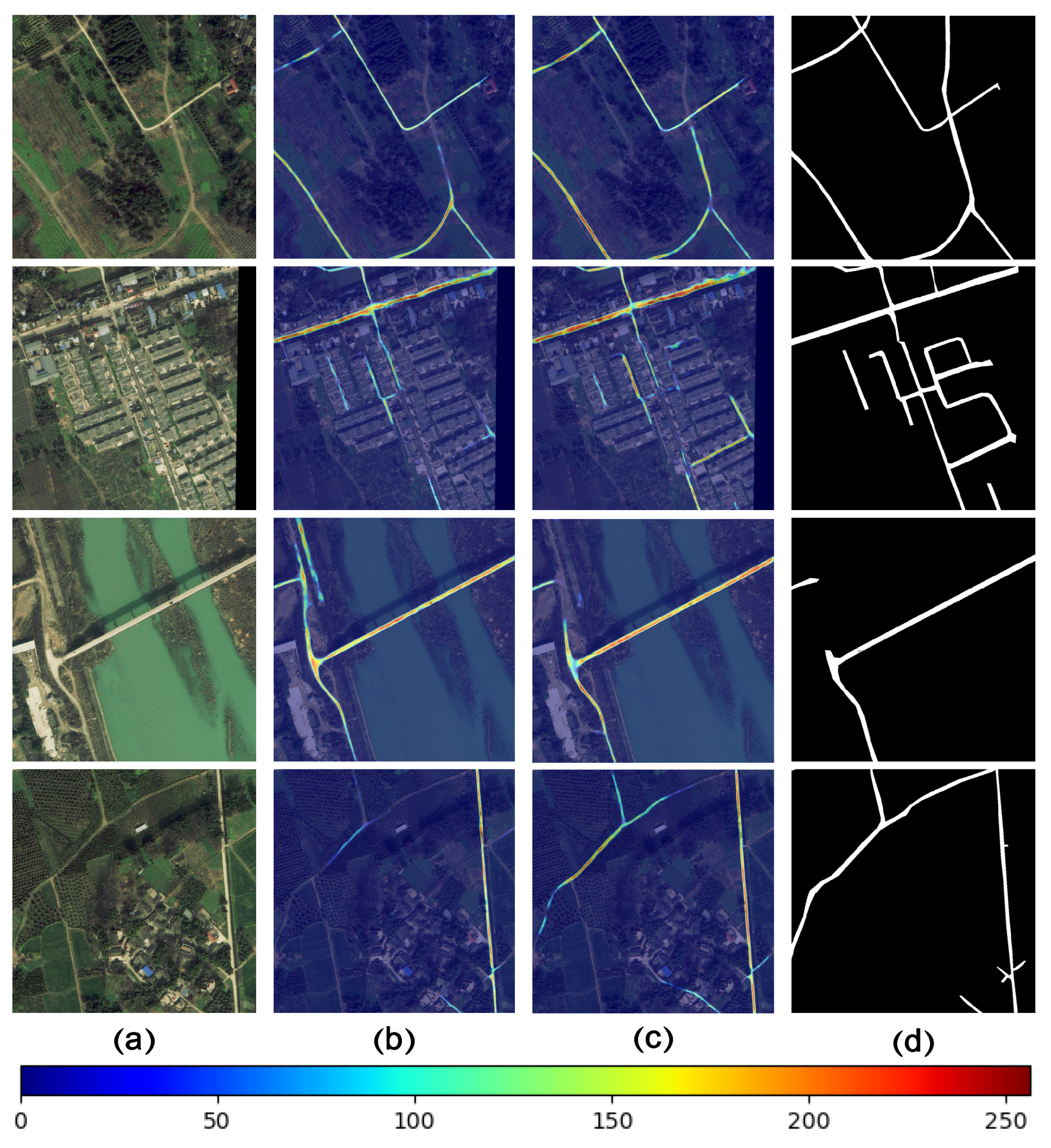
To further illustrate the advantages of MSFANet and the effectiveness of the adopted global attention mechanism, we applied Grad-CAM [47] to HRNet and MSFANet using images from the Chongzhou dataset. Grad-CAM is a visualization method based on the Class Activation Mapping (CAM) [48] visualization method, which calculates the weight of feature maps in spatial location based on gradients to express significant relationships.

Figure 14 shows the results of the visualization. The image’s highlighted region indicates the region the model cares about for a specific category. The closer to red indicates that the model cares about this region, while the darker region in the image indicates the region the model does not care. The closer to blue indicates that the model does not care about this region. In Figure 14, we see that MSFANet’s Grad-CAM mask covers the road objects better than HRNet’s Grad-mask. Furthermore, MSFANet shows higher weights on most roads, indicating that MSFANet can extract road targets more accurately.

We can observe from Figure 14 the following:

(1)

The comparison of activation maps in columns (b) and (c) shows that our proposed method can learn richer road features, including more detailed semantic representation information. Compare the activation map with the RGB images and labels in columns (a) and (d). It can be found that our model can extract more road features when the road is occluded, which improves the continuity of road extraction. Specific examples include the road in the upper left corner of the first row that is shaded by trees, and the road on the right in the second row that is shaded by building shadows.

(2)

For other features similar to roads, in our proposed method, the network has better road extract capability and will not misclassify similar features as roads. This can be demonstrated from the activation map in the third row. For the land area similar to the road in the upper left corner of the image, the activation map of MSFANet has a lower weight in this area, and no misidentification occurs, which improves the accuracy of the road extraction result.

(3)

At the position where the roads are connected, such as the lower right corner of the first row, the weight of the activation graph at the connection node is lower in the proposed method. This problem will affect the accuracy of road extraction, and it will also be solved in our follow-up research.

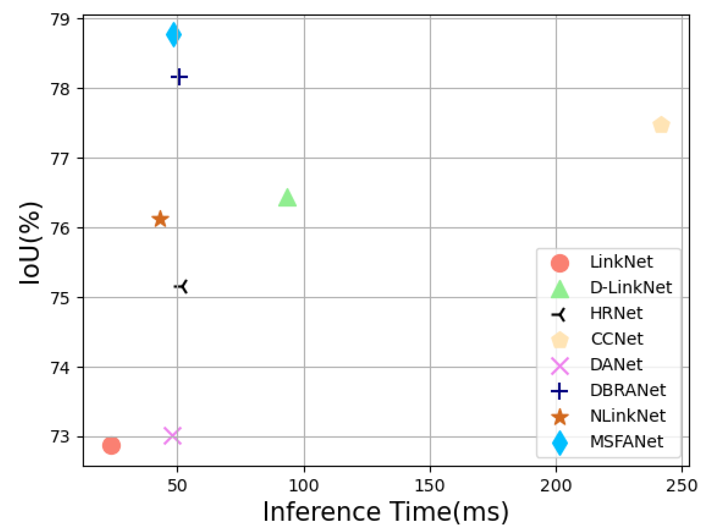
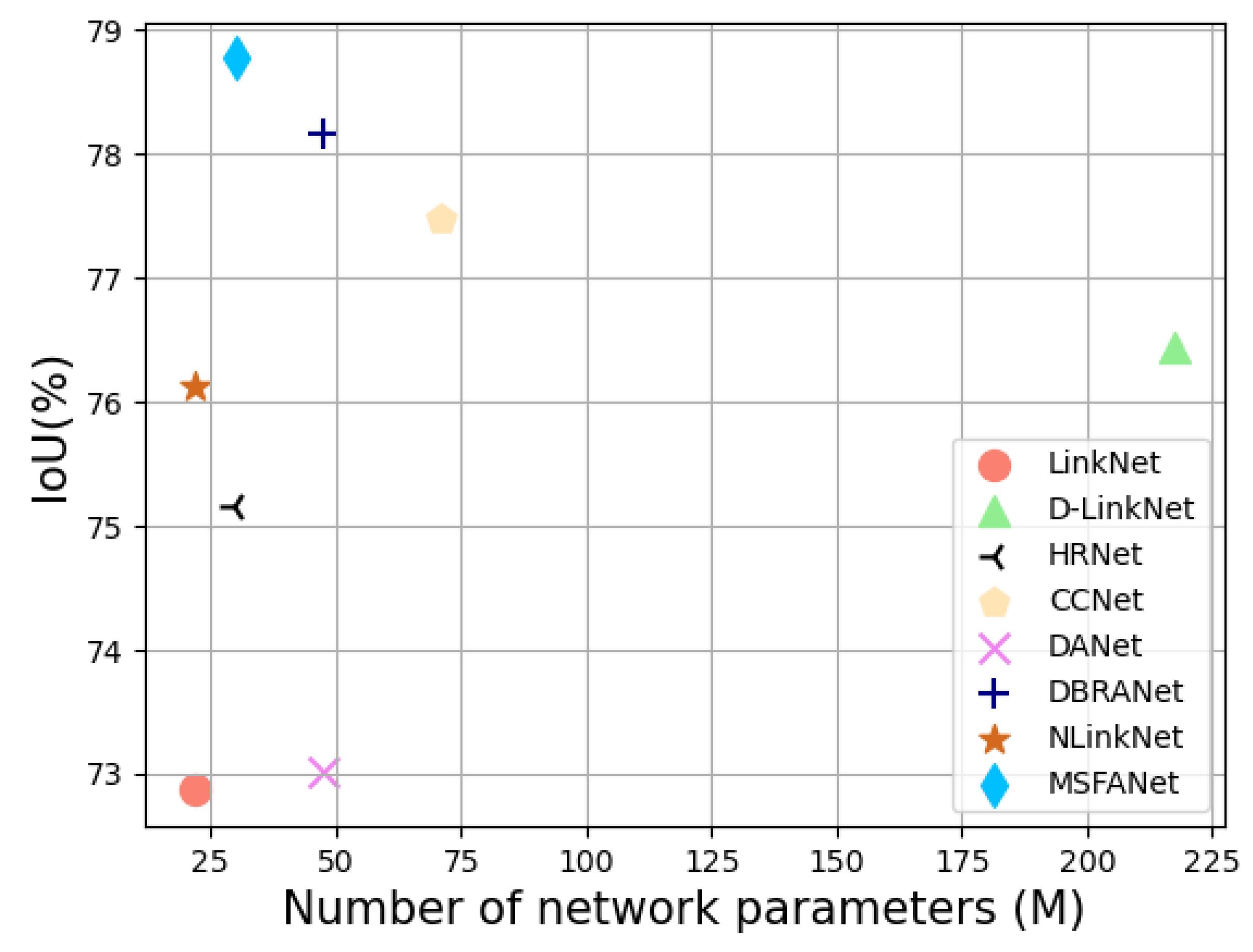
5.2. Computational Efficiency

We validated the execution time of each network we tested based on the method given by Chen et al. [49] by using the test network to predict 200 images consecutively with the batch size set to 1. The final execution time is the average of the total running time, i.e., the execution time of the network for a single image.

In addition, we calculated the number of parameters constituted by each network. We compared these data in

Table 5. Inference time, number of network parameters and IoU metrics of different methods.

Methods	Inference Time (ms/per Image)	Parameters (M)	IoU (%)
LinkNet	23.4	21.643	72.87
D-LinkNet	93.6	217.65	76.44
HRNet	51.8	29.538	75.16
CCNet	241.8	70.942	77.48
DANet	47.7	47.436	73.02
DBRANet	51.2	47.68	78.17
NLinkNet	42.8	21.82	76.12
MSFANet	48.4	30.25	78.77

, where the IoU metrics given in Table 5 are the test results of each network on the Chongzhou dataset. Compared with other methods, MSFANet is the best in terms of IoU (the best performance of road segmentation results), with a slight increase in parameters compared to HRNet. The running time (execution time) is at the same level as HRNet. Compared to other methods, the inference time of MSFANet is at the medium level.

To visualize the superiority of MSFANet in terms of computational efficiency, we plot the information in Table 5 into two graphs, Figure 15 and Figure 16. The vertical coordinates are both IoU (%), and the horizontal coordinates are the inference time and network parameters. On both graphs, the closer the coordinates are to the upper left corner indicates that the network is more accurate and has higher computational efficiency. The two tables show that MSFANet achieves a better balance of inference time, the number of parameters, and inference accuracy than other networks.

5.3. Summary of MSFANet

Considering the information and different characteristics carried by RGB images and hyperspectral images, we propose a road extraction network MSFANet, which has the following advantages:

(1)

Use RGB and hyperspectral images as the input of the road extraction network, use CFFM to calibrate RGB and hyperspectral multi-scale features, and fuse the same scale features. It avoids the loss of features caused by the mutual influence of RGB image and hyperspectral image in the feature extraction part due to the huge difference.

(2)

MSAD is designed in the decoding stage after the HRNet encoder. The information loss during upsampling is reduced by a progressive stage fusion strategy. The included dual self-attention structure can establish the global relationship between pixels in remote sensing images.

(3)

From the analysis of our experimental results, our method can extract the road features blocked by obstacles, and the ground objects that can be transplanted and similar to the road features are misclassified, which improved the extraction capabilities of the entire road extraction model.

The above experiments and analysis prove the effectiveness of our algorithm. However, our method has some shortcomings. The results cannot be extracted well at the center points where the roads are connected, such as the second and fourth rows of Figure 11. In addition, the accuracy of network extraction has improved compared with previous algorithms, but there is still a lot of room for improvement. Therefore, based on the above deficiencies, we will further improve the method to adapt to different situations in the future.

6. Conclusions

This paper proposes a multiscale fusion attention network (MSFANet) for multispectral data. We consider the importance of multiscale information and global contextual information. Different modules are designed in MSFANet to overcome the problems after introducing multispectral data. The Cross-source Feature Fusion Module aims to fuse RGB and multispectral data and resolve the errors caused by resolution and spectral differences during fusion. By introducing the Multiscale Fusion Attention Decoder, we use multiscale features and contextual image information to optimize the segmentation results. Through experimental validation and testing on our self-constructed Chongzhou and SpaceNet public datasets, MSFANet achieves a high prediction accuracy (78.77% IoU and 88.16% F1 score on the Chongzhou dataset, 61.45% IoU and 76.11% F1 score on SpaceNet dataset). In addition, inference speed and parameters (inference 48.4 ms per image and 30.25M parameters) are competitive with the compared superior methods. Through the analysis of ablation experiments, the improvement of the proposed method in road extraction is further demonstrated. The introduction of additional multispectral data can provide rich spectral information, but it needs to reintegrate and fuse features through CFFM, otherwise it will cause the decline of road extraction accuracy. In addition, MSAD’s progressive fusion strategy can reduce the information loss in the upsampling process and optimize the road extraction results. Overall, MSFANet achieves better performance than other state-of-the-art networks with a slight increase in the number of parameters than the baseline network. From the visual analysis of Grad-CAM and test results, MSFANet has better connectivity and integrity than roads extracted by other methods when the road is blocked by obstacles or the information of the features near the road is similar to the road.

In the subsequent work, we will improve the accuracy rate of the network fusion spectral information and introduce more remote sensing data with different modes, such as Synthetic Aperture Radar (SAR) and Digital Surface Model (DSM). Future research will be conducted on multi-source data fusion with semantic segmentation as the core.

References

1. Zhou, M.; Sui, H.; Chen, S.; Wang, J.; Chen, X. BT-RoadNet: A boundary and topologically-aware neural network for road extraction from high-resolution remote sensing imagery. ISPRS J. Photogramm. Remote Sens. 2020, 168, 288–306. [Google Scholar] [CrossRef]
2. Bachagha, N.; Wang, X.; Luo, L.; Li, L.; Khatteli, H.; Lasaponara, R. Remote sensing and GIS techniques for reconstructing the military fort system on the Roman boundary (Tunisian section) and identifying archaeological sites. Remote Sens. Environ. 2020, 236, 111418. [Google Scholar] [CrossRef]
3. Jia, J.; Sun, H.; Jiang, C.; Karila, K.; Karjalainen, M.; Ahokas, E.; Khoramshahi, E.; Hu, P.; Chen, C.; Xue, T.; et al. Review on active and passive remote sensing techniques for road extraction. Remote Sens. 2021, 13, 4235. [Google Scholar] [CrossRef]
4. Xu, Z.; Liu, Y.; Gan, L.; Hu, X.; Sun, Y.; Liu, M.; Wang, L. csBoundary: City-Scale Road-Boundary Detection in Aerial Images for High-Definition Maps. IEEE Robot. Autom. Lett. 2022, 7, 5063–5070. [Google Scholar] [CrossRef]
5. Li, Q.; Chen, L.; Li, M.; Shaw, S.L.; Nüchter, A. A sensor-fusion drivable-region and lane-detection system for autonomous vehicle navigation in challenging road scenarios. IEEE Trans. Veh. Technol. 2013, 63, 540–555. [Google Scholar] [CrossRef]
6. Aboah, A. A Vision-Based System for Traffic Anomaly Detection Using Deep Learning and Decision Trees. In Proceedings of the IEEE/CVF Conference on Computer Vision and Pattern Recognition (CVPR) Workshops, Nashville, TN, USA, 19–25 June 2021; pp. 4207–4212. [Google Scholar]
7. Bonnefon, R.; Dhérété, P.; Desachy, J. Geographic information system updating using remote sensing images. Pattern Recognit. Lett. 2002, 23, 1073–1083. [Google Scholar] [CrossRef]
8. Lian, R.; Wang, W.; Mustafa, N.; Huang, L. Road extraction methods in high-resolution remote sensing images: A comprehensive review. IEEE J. Sel. Top. Appl. Earth Obs. Remote Sens. 2020, 13, 5489–5507. [Google Scholar] [CrossRef]
9. Stoica, R.; Descombes, X.; Zerubia, J. A Gibbs point process for road extraction from remotely sensed images. Int. J. Comput. Vis. 2004, 57, 121–136. [Google Scholar] [CrossRef]
10. Bacher, U.; Mayer, H. Automatic road extraction from multispectral high resolution satellite images. In Proceedings of the CMRT05, Vienna, Austria, 29–30 August 2005; Volume 36. [Google Scholar]
11. Mohammadzadeh, A.; Tavakoli, A.; Valadan Zoej, M.J. Road extraction based on fuzzy logic and mathematical morphology from pan-sharpened Ikonos images. Photogramm. Rec. 2006, 21, 44–60. [Google Scholar] [CrossRef]
12. Maurya, R.; Gupta, P.; Shukla, A.S. Road extraction using k-means clustering and morphological operations. In Proceedings of the 2011 International Conference on Image Information Processing, Shimla, Himachal Pradesh, India, 3–5 November 2011; pp. 1–6. [Google Scholar]
13. Song, M.; Civco, D. Road extraction using SVM and image segmentation. Photogramm. Eng. Remote Sens. 2004, 70, 1365–1371. [Google Scholar] [CrossRef] [Green Version]
14. Amo, M.; Martínez, F.; Torre, M. Road extraction from aerial images using a region competition algorithm. IEEE Trans. Image Process. 2006, 15, 1192–1201. [Google Scholar] [CrossRef]
15. Yager, N.; Sowmya, A. Support vector machines for road extraction from remotely sensed images. In Proceedings of the Computer Analysis of Images and Patterns: 10th International Conference, CAIP 2003, Groningen, The Netherlands, 25–27 August 2003; Springer: Berlin/Heidelberg, Germany, 2003; pp. 285–292. [Google Scholar]
16. Storvik, G.; Fjortoft, R.; Solberg, A.H.S. A Bayesian approach to classification of multiresolution remote sensing data. IEEE Trans. Geosci. Remote Sens. 2005, 43, 539–547. [Google Scholar] [CrossRef]
17. Long, J.; Shelhamer, E.; Darrell, T. Fully convolutional networks for semantic segmentation. In Proceedings of the IEEE Conference on Computer Vision and Pattern Recognition, Boston, MA, USA, 7–12 June 2015; pp. 3431–3440. [Google Scholar]
18. Chaurasia, A.; Culurciello, E. Linknet: Exploiting encoder representations for efficient semantic segmentation. In Proceedings of the 2017 IEEE Visual Communications and Image Processing (VCIP), St. Petersburg, FL, USA, 10–13 December 2017; pp. 1–4. [Google Scholar]
19. Ronneberger, O.; Fischer, P.; Brox, T. U-net: Convolutional networks for biomedical image segmentation. In Proceedings of the International Conference on Medical Image Computing and Computer-Assisted Intervention, Munich, Germany, 5–9 October 2015; Springer: Berlin/Heidelberg, Germany, 2015; pp. 234–241. [Google Scholar]
20. Ke, K.; Zhao, Y.; Jiang, B.; Cheng, T.; Xiao, B.; Liu, D.; Yadong, M.; Wang, X.; Liu, W.; Wang, J. High-resolution representations for labeling pixels and regions. In Proceedings of the IEEE International Conference on Computer Vision, Seoul, Republic of Korea, 27 October–2 November 2019. [Google Scholar]
21. Wang, Y.; Peng, Y.; Li, W.; Alexandropoulos, G.C.; Yu, J.; Ge, D.; Xiang, W. DDU-Net: Dual-decoder-U-Net for road extraction using high-resolution remote sensing images. IEEE Trans. Geosci. Remote Sens. 2022, 60, 1–12. [Google Scholar] [CrossRef]
22. Yang, M.; Yuan, Y.; Liu, G. SDUNet: Road extraction via spatial enhanced and densely connected UNet. Pattern Recognit. 2022, 126, 108549. [Google Scholar] [CrossRef]
23. Yang, X.; Li, X.; Ye, Y.; Lau, R.Y.; Zhang, X.; Huang, X. Road detection and centerline extraction via deep recurrent convolutional neural network U-Net. IEEE Trans. Geosci. Remote Sens. 2019, 57, 7209–7220. [Google Scholar] [CrossRef]
24. Wan, J.; Xie, Z.; Xu, Y.; Chen, S.; Qiu, Q. DA-RoadNet: A dual-attention network for road extraction from high resolution satellite imagery. IEEE J. Sel. Top. Appl. Earth Obs. Remote Sens. 2021, 14, 6302–6315. [Google Scholar] [CrossRef]
25. Huan, H.; Sheng, Y.; Zhang, Y.; Liu, Y. Strip Attention Networks for Road Extraction. Remote Sens. 2022, 14, 4516. [Google Scholar] [CrossRef]
26. Ma, W.; Karakuş, O.; Rosin, P.L. AMM-FuseNet: Attention-based multi-modal image fusion network for land cover mapping. Remote Sens. 2022, 14, 4458. [Google Scholar] [CrossRef]
27. Zhao, H.; Shi, J.; Qi, X.; Wang, X.; Jia, J. Pyramid scene parsing network. In Proceedings of the IEEE Conference on Computer Vision and Pattern Recognition, Honolulu, HI, USA, 21–26 July 2017; pp. 2881–2890. [Google Scholar]
28. Chen, L.C.; Zhu, Y.; Papandreou, G.; Schroff, F.; Adam, H. Encoder-decoder with atrous separable convolution for semantic image segmentation. In Proceedings of the European Conference on Computer Vision (ECCV), Munich, Germany, 8–14 September 2018; pp. 801–818. [Google Scholar]
29. Zhou, L.; Zhang, C. Linknet with pretrained encoder and dilated convolution for high resolution satellite imagery road extraction. In Proceedings of the CVF Conference on Computer Vision and Pattern Recognition Workshops (CVPRW), Salt Lake City, UT, USA, 18–22 June 2018; pp. 192–1924. [Google Scholar]
30. He, S.; Bastani, F.; Jagwani, S.; Alizadeh, M.; Balakrishnan, H.; Chawla, S.; Elshrif, M.M.; Madden, S.; Sadeghi, M.A. Sat2graph: Road graph extraction through graph-tensor encoding. In Proceedings of the European Conference on Computer Vision, Glasgow, UK, 23–28 August 2020; Springer: Berlin/Heidelberg, Germany, 2020; pp. 51–67. [Google Scholar]
31. Xie, Y.; Miao, F.; Zhou, K.; Peng, J. HsgNet: A road extraction network based on global perception of high-order spatial information. ISPRS Int. J. Geo Inf. 2019, 8, 571. [Google Scholar] [CrossRef] [Green Version]
32. Chen, S.B.; Ji, Y.X.; Tang, J.; Luo, B.; Wang, W.Q.; Lv, K. DBRANet: Road extraction by dual-branch encoder and regional attention decoder. IEEE Geosci. Remote Sens. Lett. 2021, 19, 1–5. [Google Scholar] [CrossRef]
33. Wang, Y.; Seo, J.; Jeon, T. NL-LinkNet: Toward lighter but more accurate road extraction with nonlocal operations. IEEE Geosci. Remote Sens. Lett. 2021, 19, 1–5. [Google Scholar] [CrossRef]
34. Wang, X.; Girshick, R.; Gupta, A.; He, K. Non-local neural networks. In Proceedings of the IEEE Conference on Computer Vision and Pattern Recognition, Salt Lake City, UT, USA, 18–22 June 2018; pp. 7794–7803. [Google Scholar]
35. Hu, J.; Shen, L.; Sun, G. Squeeze-and-excitation networks. In Proceedings of the IEEE Conference on Computer Vision and Pattern Recognition, Salt Lake City, UT, USA, 18–22 June 2018; pp. 7132–7141. [Google Scholar]
36. Huang, Z.; Wang, X.; Huang, L.; Huang, C.; Wei, Y.; Liu, W. Ccnet: Criss-cross attention for semantic segmentation. In Proceedings of the IEEE/CVF International Conference on Computer Vision, Seoul, Republic of Korea, 27 October–2 November 2019; pp. 603–612. [Google Scholar]
37. Fu, J.; Liu, J.; Tian, H.; Li, Y.; Bao, Y.; Fang, Z.; Lu, H. Dual attention network for scene segmentation. In Proceedings of the IEEE/CVF Conference on Computer Vision and Pattern Recognition, Long Beach, CA, USA, 15–20 June 2019; pp. 3146–3154. [Google Scholar]
38. Li, H.; Xiong, P.; An, J.; Wang, L. Pyramid attention network for semantic segmentation. In Proceedings of the British Machine Vision Conference, Newcastle, UK, 3–6 September 2018; p. 285. [Google Scholar]
39. Rudner, T.G.; Rußwurm, M.; Fil, J.; Pelich, R.; Bischke, B.; Kopačková, V.; Biliński, P. Multi3net: Segmenting flooded buildings via fusion of multiresolution, multisensor, and multitemporal satellite imagery. In Proceedings of the AAAI Conference on Artificial Intelligence, Honolulu, HI, USA, 27 January–1 February 2019; Volume 33, pp. 702–709. [Google Scholar]
40. Ma, X.; Zhang, X.; Pun, M.O. A crossmodal multiscale fusion network for semantic segmentation of remote sensing data. IEEE J. Sel. Top. Appl. Earth Obs. Remote Sens. 2022, 15, 3463–3474. [Google Scholar] [CrossRef]
41. Lei, T.; Li, L.; Lv, Z.; Zhu, M.; Du, X.; Nandi, A.K. Multi-modality and multi-scale attention fusion network for land cover classification from VHR remote sensing images. Remote Sens. 2021, 13, 3771. [Google Scholar] [CrossRef]
42. Sun, Y.; Fu, Z.; Sun, C.; Hu, Y.; Zhang, S. Deep multimodal fusion network for semantic segmentation using remote sensing image and LiDAR data. IEEE Trans. Geosci. Remote Sens. 2021, 60, 1–18. [Google Scholar] [CrossRef]
43. Cao, Z.; Diao, W.; Sun, X.; Lyu, X.; Yan, M.; Fu, K. C3net: Cross-modal feature recalibrated, cross-scale semantic aggregated and compact network for semantic segmentation of multi-modal high-resolution aerial images. Remote Sens. 2021, 13, 528. [Google Scholar] [CrossRef]
44. De Carvalho, O.L.F.; de Carvalho Júnior, O.A.; De Albuquerque, A.O.; Santana, N.C.; Borges, D.L.; Luiz, A.S.; Gomes, R.A.T.; Guimarães, R.F. Multispectral panoptic segmentation: Exploring the beach setting with worldview-3 imagery. Int. J. Appl. Earth Obs. Geoinf. 2022, 112, 102910. [Google Scholar] [CrossRef]
45. Van Etten, A.; Lindenbaum, D.; Bacastow, T.M. Spacenet: A remote sensing dataset and challenge series. arXiv 2018, arXiv:1807.01232. [Google Scholar]
46. Batra, A.; Singh, S.; Pang, G.; Basu, S.; Jawahar, C.; Paluri, M. Improved road connectivity by joint learning of orientation and segmentation. In Proceedings of the IEEE/CVF Conference on Computer Vision and Pattern Recognition, Long Beach, CA, USA, 15–20 June 2019; pp. 10385–10393. [Google Scholar]
47. Selvaraju, R.R.; Cogswell, M.; Das, A.; Vedantam, R.; Parikh, D.; Batra, D. Grad-CAM: Visual Explanations From Deep Networks via Gradient-Based Localization. In Proceedings of the IEEE International Conference on Computer Vision (ICCV), Venice, Italy, 22–29 October 2017. [Google Scholar]
48. Zhou, B.; Khosla, A.; Lapedriza, A.; Oliva, A.; Torralba, A. Learning deep features for discriminative localization. In Proceedings of the IEEE Conference on Computer Vision and Pattern Recognition, Las Vegas, NV, USA, 26 June–1 July 2016; pp. 2921–2929. [Google Scholar]
49. Chu, X.; Chen, L.; Yu, W. NAFSSR: Stereo Image Super-Resolution Using NAFNet. In Proceedings of the IEEE/CVF Conference on Computer Vision and Pattern Recognition, New Orleans, LA, USA, 18–24 June 2022; pp. 1239–1248. [Google Scholar]
Figure 1. The structure of HRNet, the rectangular blocks represent the feature map, the color of the rectangular blocks illustrates the different scale branches in HRNet, and ‘→’ refers to convolution operations.
Remotesensing 15 01978 g001
Figure 2. Explains how HRNet fuses information from different scales; Conv (3 × 3) is the convolution of stride 3 × 3 and upsampling (1 × 1) is the combination of nearest neighbor interpolation upsampling and 1 × 1 convolution.
Remotesensing 15 01978 g002
Figure 3. The overall structure of MSFANet.
Remotesensing 15 01978 g003
Figure 4. The process of Cross-source Feature Recalibration Module (CFRM).
Remotesensing 15 01978 g004
Figure 5. Illustration of the structure of PAM.
Remotesensing 15 01978 g005
Figure 6. Illustration of the structure of CAM.
Remotesensing 15 01978 g006
Figure 7. Illustration of the structure of the Smooth Fusion Module.
Remotesensing 15 01978 g007
Figure 8. Overview of the Chongzhou dataset area from (a) the whole area of the Chongzhou data, the box is the sub-area of the display; (b) RGB-pansharpening image of sub-area; (c) panchromatic band image of sub-area; (d) coastal blue band image of sub-area; (e) blue band image of sub-area; (f) green band image of sub-area; (g) yellow band image of sub-area; (h) red band image of sub-area; (i) red edge band image of sub-area; (j) near-IR1 band image of sub-area; (k) near-IR2 band image of sub-area.
Remotesensing 15 01978 g008
Figure 9. Overview of the SpaceNet dataset area from (a,b) Khartoum; (c,d) Shanghai; (e,f) Paris; (g,h) Vegas.
Remotesensing 15 01978 g009
Figure 10. Results of road extraction on the Chongzhou dataset. (a) RGB satellite imagery. (b) Ground truth. (c) LinkNet. (d) D-LinkNet. (e) HRNet. (f) CCNet. (g) DANet. (h) DBRANet. (i) NL-LinkNet. (j) MSFANet.
Remotesensing 15 01978 g010
Figure 11. Results of road extraction on the SpaceNet dataset. (a) RGB satellite imagery. (b) Ground truth. (c) LinkNet. (d) D-LinkNet. (e) HRNet. (f) CCNet. (g) DANet. (h) DBRANet. (i) NL-LinkNet. (j) MSFANet.
Remotesensing 15 01978 g011
Figure 12. Results of ablation experiments on the Chongzhou dataset. (a) RGB satellite imagery. (b) Ground truth. (c) HRNet. (d) HRNet with multispectral input. (e) MSFANet without multispectral input and CFFM. (f) MSFANet without multispectral input. (g) MSFANet without MFAD module. (h) MSFANet.
Remotesensing 15 01978 g012
Figure 13. Results of ablation experiments on the SpaceNet dataset. (a) RGB satellite imagery. (b) Ground truth. (c) HRNet. (d) HRNet with multispectral input. (e) MSFANet without multispectral input and CFFM. (f) MSFANet without multispectral input. (g) MSFANet without MFAD module. (h) MSFANet.
Remotesensing 15 01978 g013
Figure 14. Grad-CAM visualization results for (a) the RGB image, (b) the result of fusing the RGB image with HRNet’s Grad-CAM mask, (c) the result of fusing the RGB image with MSFANet’s Grad-CAM mask and (d) the label.
Remotesensing 15 01978 g014
Figure 15. The inference time and IoU of each network.
Remotesensing 15 01978 g015
Figure 16. Number of parameters and IoU for each network.
Remotesensing 15 01978 g016