Convolutional Neural Network Maps Plant Communities in Semi-Natural Grasslands Using Multispectral Unmanned Aerial Vehicle Imagery

Abstract

Semi-natural grasslands (SNGs) are an essential part of European cultural landscapes. They are an important habitat for many animal and plant species and offer a variety of ecological functions. Diverse plant communities have evolved over time depending on environmental and management factors in grasslands. These different plant communities offer multiple ecosystem services and also have an effect on the forage value of fodder for domestic livestock. However, with increasing intensification in agriculture and the loss of SNGs, the biodiversity of grasslands continues to decline. In this paper, we present a method to spatially classify plant communities in grasslands in order to identify and map plant communities and weed species that occur in a semi-natural meadow. For this, high-resolution multispectral remote sensing data were captured by an unmanned aerial vehicle (UAV) in regular intervals and classified by a convolutional neural network (CNN). As the study area, a heterogeneous semi-natural hay meadow with first- and second-growth vegetation was chosen. Botanical relevés of fixed plots were used as ground truth and independent test data. Accuracies up to 88% on these independent test data were achieved, showing the great potential of the usage of CNNs for plant community mapping in high-resolution UAV data for ecological and agricultural applications.

1. Introduction

In Central Europe, semi-natural grasslands (SNGs) are an essential part of ancient cultural landscapes. They have developed over centuries of anthropogenic land use by grazing and mowing [1,2]. Until the 19th century, most European SNGs were used as pastures, whereas hay meadows developed mainly over the last 100 to 150 years [1]. The highest diversity of species and plant communities in grasslands was reached in the middle of the 19th century [2]. Increasing intensification of land use, however, has led to decreasing species richness, especially since the 1950s [3,4]. Furthermore, the area used as grasslands in Germany decreased continuously from the 1970s until 2013. Since then, a reform of the common agricultural policy of the European Union (EU) regulates the transformation of grasslands into arable land [5]. Furthermore, subsidies for biodiversity-friendly use of grasslands were included as greening in the subsidy scheme of the EU [1]. For example, in Lower Saxony subsidies were granted for low-intensity use of high-nature-value grasslands [6]. This included a ban on mineral nitrogen fertilizers or pesticides and a prescribed earliest date for mowing.

Contrastingly, agriculturally improved grasslands are used, e.g., for dairy farming. Here, a high energy and protein concentration in the forage is required for increasing the milk production of the individual animal [7]. This is achieved by special grass cultivars and fertilizer application, which increase the number of mowings possible per year. Yield from SNG is not always processed into silage for milk production but can also be cut once or twice a year to produce hay in the traditional way, which maintains species richness [8]. If this hay is not fed to cattle or sheep but to horses, special importance must be paid to its plant species composition. Horses do not tolerate some Lolium or Festuca species due to their high fructose content [9,10]. Furthermore, these grass species may contain endophytic fungi that make them highly resistant to environmental conditions [11] and are harmful to horses but not ruminants [12]. Apart from their usage as fodder for meat, dairy, and wool production, SNGs’ multiple ecosystem services include good groundwater quality and quantity, water flow regulation, carbon storage, mitigation of greenhouse gas fluxes, and erosion prevention, as well as cultural and health values. [13]. Furthermore, they are a habitat for many plant and animal species [13]. Both ecosystem services and habitat conditions of grasslands cannot be determined by mapping land use or land cover type only, because of the spatial variability in the biophysical variables [14]. Ecosystem services can vary over land use or land cover types [15], as species abundance and diversity in grassland plant communities influence their provision [16]. The composition of plant communities can change due to spatiotemporal dynamics, like water balance in the soil, light availability, or management [17].

To monitor vegetation structure and species composition, field-based methods in the form of phytosociological relevés are commonly used but are rather time-consuming [18,19]. In contrast, remote sensing is a cost-effective and non-destructive alternative, which is increasingly applied to get vegetation data of large-scale areas or areas showing spatiotemporal dynamics [20,21,22,23]. On a large scale, various remote sensing systems can be used to classify plant communities in grasslands. The authors of [24,25] used spaceborne data as a combination of multispectral and/or radar time series, whereas [20] analyzed airborne LiDAR. Over the last years, UAVs are increasingly used for ecological tasks on a smaller scale [26]. As an example, they were used in grasslands for the estimation of biodiversity [27], species and vegetation functional groups classification [23,28,29], forage quality, and biomass prediction [30,31] as well as for the detection of weed plants [32,33]. Various methodological approaches are suitable for the classification of plant communities in remote sensing data. To use the influence of phenology, some studies use multitemporal data for species and plant community classification [23,29]. The authors of [24,29] used machine learning techniques such as support vector machine and random forest for the classification of species and plant communities in grasslands. The authors of [34,35] tested the suitability of convolutional neural networks (CNNs) for their classification of plant communities in shrublands and forests. Recently, CNNs have been increasingly applied for the analysis of remote sensing data [36], but also specifically in vegetation remote sensing [22]. CNNs are particularly suitable for the detection of spatial patterns. As plant communities in grasslands are formed by plants of different heights and shapes, the spatial pattern is, in addition to spectral information, a strong feature for separation.

In our study, plant communities in a semi-natural hay meadow in northwestern Germany were classified with UAV imagery using CNNs. The aim is to use CNNs (1) to analyze the spatial distribution of the plant community composition before the first and second cut of the grassland vegetation and (2) to map the distribution of weed species with low forage value. Thereby, (3) the usage of mono- and multitemporal data for the mapping of plant communities with respect to the phenological phases is compared.

2. Material and Methods

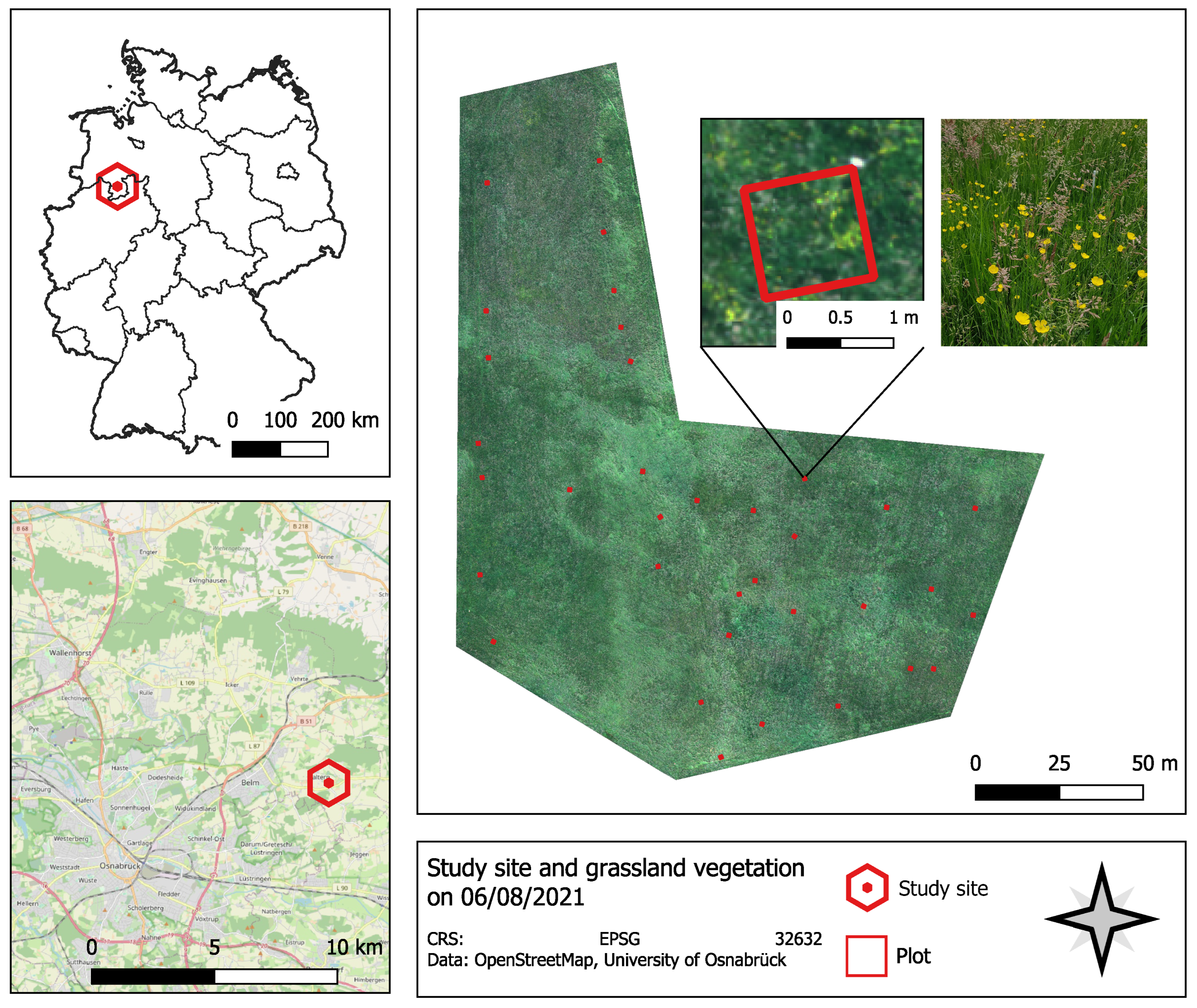
2.1. Study Site

This study focuses on a 2.3 ha semi-natural meadow in the Osnabrück district, Lower Saxony, Germany (52.18°N, 8.10°E), as visible in Figure 1. According to the official soil survey map [37], the soil is predominantly gley, with part of the northern area being plaggic anthrosol. The climate is temperate oceanic, with an annual precipitation of 835 mm and a mean air temperature of 8.8 °C [38].

This survey covers the first growth ($G_1$) of plants from the beginning of May 2021 until the first mowing in the middle of June 2021, and the second growth ($G_2$) until the second mowing at the end of August 2021. The SNG can be assigned to the class Molino-Arrhenatheretea and the order Arrhenatheretalia [2]. Over the past 5 years, the study site was used twice a year for hay production according to the agri-environmental measure for low-intensity use of grasslands in Lower Saxony GL11 [6]. Before that, it had been used as a cattle pasture for about 30 years and a heterogeneous structure of plant communities had developed.

2.2. Data and Preprocessing

2.2.1. UAV Image Data

UAV data for this study were captured using a DJI Phantom 4 multispectral. The camera system offers five single-spectral cameras (blue (450 ± 16 nm), green (560 ± 16 nm), red (650 ± 16 nm), red edge (730 ± 16 nm), and infrared (840 ± 26 nm)) as well as an RGB camera. Each sensor has a resolution of 2.08 Megapixels and a focal length of 5.74 mm. Due to the flight altitude of 35 m a resolution of less then two centimeters was achieved. Images were taken on four dates during the first growth $G_1$ (

Table 1. Growth, observation dates and times, number of botanically observed plots, weather conditions, and wind speed during the flights.

Growth	ID	Date	Time of Flight	No. of Plots	Weather Conditions	Wind Speed
Growth 1	$G_1{T}_0$	05/03/2021	10:58 a.m.–11:24 a.m.	0	closed cloud cover	2 m/s
Growth 1	$G_1{T}_1$	05/12/2021	2:47 p.m.–3:11 p.m.	30	closed cloud cover	5.7 m/s
Growth 1	$G_1{T}_2$	05/28/2021	1:59 p.m.–2:28 p.m.	30	sunny with a few clouds	6.4 m/s
Growth 1	$G_1{T}_3$	06/08/2021	2:06 p.m.–2:30 p.m.	29	closed cloud cover	2.9 m/s
Growth 2	$G_2{T}_0$	06/25/2021	12:45 a.m.–1:22 p.m.	0	sunny and cloudless	3.9 m/s
Growth 2	$G_2{T}_1$	07/12/2021	11:22 a.m.–11:47 a.m.	35	sunny and cloudless	1.6 m/s
Growth 2	$G_2{T}_2$	07/27/2021	11:22 a.m.–11:49 a.m.	35	first sunny, then cloudy	2.2 m/s
Growth 2	$G_2{T}_3$	08/06/2021	11:13 a.m.–11:44 a.m.	35	closed cloud cover	2.2 m/s

, $G_1{T}_0$-$G_1{T}_3$), and four dates during the second growth $G_2$ (Table 1, $G_2{T}_0$-$G_2{T}_3$). Flights took place during noon (between 11 am and 3 pm) to minimize the influence of shadows. Each flight took about 30 to 35 min. The weather conditions on the observation days were inconsistent (see Table 1). Eight to ten field targets were placed before the flights and used as ground control points (GCPs). The center of each target was located using a differential GPS (bi-frequent GNSS receiver). On each observation day, around 350 images per channel were made with a front and side overlap of 70%. The images were stitched to a multispectral orthomosaic using Agisoft Metashape software (version V1.7.2), georeferenced using the GCPs, and clipped to the extent of the study site.

2.2.2. Vegetation Surveys in the Field

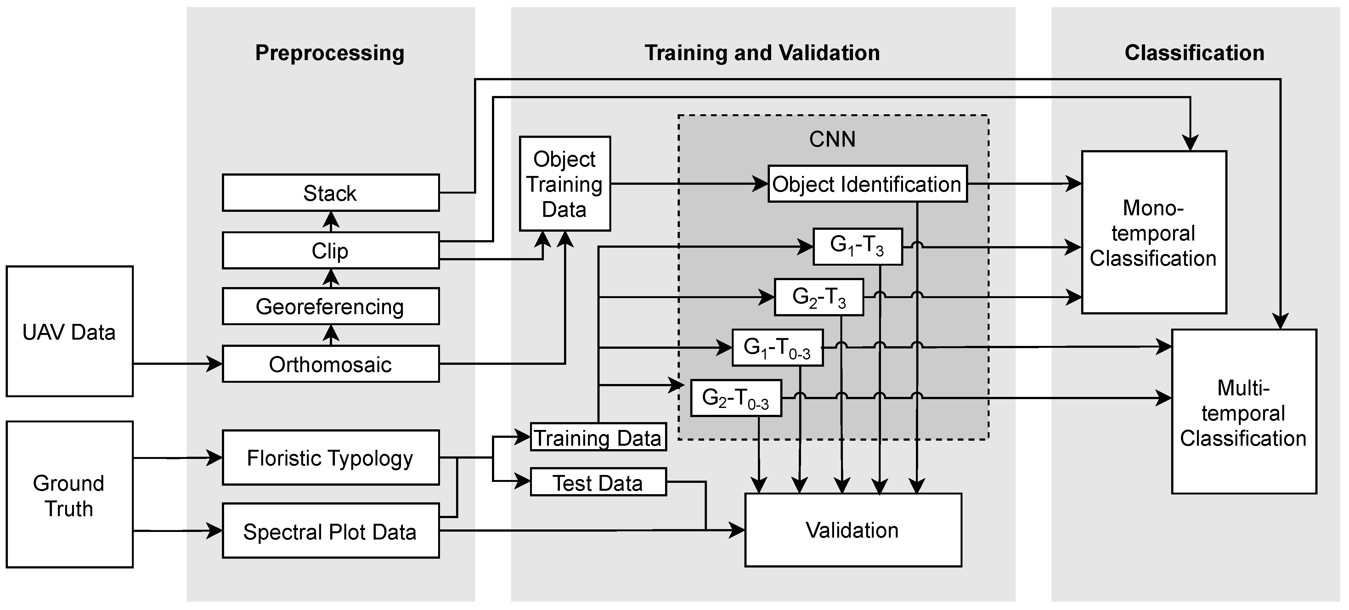
A total of 30 plots were stratified randomly distributed and marked during the first growth. For this, homogeneous areas were visually identified based on dominant species and 1 m × 1 m plots were placed. The four corner points of a plot were captured using a differential GPS. The area of one square meter is less than the minimum area of 10–25 m${}^2$ recommended for botanical examinations in pastures [18], but to generate a variety of training data, a smaller plot size was chosen. At date $G_1{T}_3$, plot 26 was damaged and some of the vegetation was removed, leaving only 29 plots to be recorded (Table 1). After the first mowing, the existing plots were marked again and extended by five more plots. On six observation days, $T_1\text{–}{T}_3$ in each growth, vegetation relevés were recorded by visual cover estimation after the UAV flight using the scale of [39]. As many characteristic and indicative species were not fully grown at both $G_1{T}_0$ (early in the vegetation period) and $G_2{T}_0$ (immediately after mowing), no botanical data were recorded at these times.

2.3. Methodology

2.3.1. Analysis of Vegetation Data

We used the nomenclature for plant species according to [40]. Vegetation units (VUs) were formed by sorting the relevés in each growth by similar composition. The species in these VUs were sorted to form species groups. These groups show dominant species within the VUs. Four VUs were formed in the first growth, and three in the second. The plant species of a VU were listed in terms of their frequency to validate the separation into plant communities with the help of Ellenberg indicator values (EIV): soil moisture number (M, 1 = strong soil dryness, 5 = moist, 9 = wet, 12 = underwater), soil reaction number (R, 1 = extremely acidic, 5 = mildly acidic, 9 = alkaline) and nutrient number (N, 1 = least, 5 = average, 9 = excessive supply) [41]. The weighted means were calculated using the indicator values presented. The forage value, considering for example the protein and mineral content of the VUs, was determined using the values of [42].

2.3.2. Training and Test Data

The data used to train the CNN were obtained from the orthomosaics by visual interpretation and knowledge of the vegetation composition and regarding the time series. Since the plots were placed in homogeneous areas, it was assumed that the adjacent areas were dominated by the same plant community. Further training data for the VU dominated by Rumex obtusifolius could be obtained on the whole area, as this plant was easily identifiable. For each VU except for the one dominated by Rumex obtusifolius, 100 non-overlapping samples were taken in the homogeneous area around the observed plots. Only 30 samples of Rumex obtusifolius were taken because the plants in the study site were limited. Each training sample had an actual size of 1 × 1 m, according to the size of the plots, which corresponds to a size of 53 ± 1 × 53 ± 1 pixels. Following common standards to enhance the number of training samples [43], they were augmented as follows: Resampling to 64 × 64 pixels with nearest neighbor, rotating and flipping, and sporadic application of a median filter (kernel size 3) to add blur [44]. For use in the CNN, a random 75% (random state = 42) of the training data were used for training, the remaining 25% was used as a dependent test set for validation.

The spectral data of the observed plots were clipped and used for independent validation. Since the plot orientation does not correspond to the raster, the clipped plot samples were rotated and resampled. To avoid misclassification, a CNN with the same structure as shown in

Table 2. Architecture of the used CNN.

Layer	Parameter
Input	64 × 64 × 5
Conv2D_1	Filter: 32, Kernel: 3 × 3, Strides: 2 × 2, Activation: ReLU
BatchNormalization	-
Dropout	0.1
Conv2D_2	Filter: 128, Kernel: 3 × 3, Strides: 2 × 2, Activation: ReLU
BatchNormalization	-
Dropout	0.1
Reshape	-
FullyConnected_1	Dense: 64, Activation: ReLU
BatchNormalization	-
Dropout	0.2
FullyConnected_2	Dense: n, Activation: Softmax

was trained to binary classify objects that are not part of the vegetation. For this, training data were collected from fence posts, bare soil, fawns, molehills, and targets and augmented as described above.

2.3.3. CNN

The structure of CNNs is inspired by the biological structure of a brain. Both consist of repeating layers of simple and complex cells to solve segmentation, detection, and localization tasks [36]. The first CNNs were presented in the late 1980s, e.g., by [45] for the recognition of handwriting digits. Nowadays, they are the leading model for image classification, detection, and recognition tasks [36]. Each convolutional layer of a CNN extracts features and local conjunctions of the previous layer with weighted neurons. For this, kernels of a certain size are used to pass over the feature map or filter, and forwarded to a nonlinear activation function, e.g., rectified linear units (ReLU) [46]. There are two commonly applied techniques to simplify and aggregate the outputs of a convolutional layer. The first is to insert pooling layers. For this, features are merged (e.g., using the maximum or average value) with a pooling kernel to reduce the spacial resolution and decorrelate the features [47]. The second is the use of strides instead of pooling. Strides describe the step size of the kernel, and by increasing their size, the spatial resolution can be reduced. They are useful when input sizes are small [48] and are also utilized in more complex architectures such as ResNet to achieve higher accuracy and increase the training and classification speed [49]. Several convolutional layers in series can derive abstract features of the input. Fully connected layers of neurons and weights, as in standard neural networks, are attached to this to interpret these abstract features. For classification problems, in general a softmax function is used as the activation function in the last fully connected layer [46].

The CNN applied in this study was created with TensorFlow’s Keras Python API (version 2.3.1). Its structure is shown in Table 2. Two convolutional layers, the first with 32 filters, the second with 128 filters, and two fully connected layers, the first of size 64, the second of size n, which is the number of output classes, were implemented. A softmax activation function in combination with a cross-entropy loss function (also known as categorical cross-entropy loss [50]) was used in this last layer to give a probability for the predicted output. The model utilizes Adam as an optimizer because it showed good results for CNNs [51]. Strides are applied within the convolutional layers to aggregate the features. A ReLU activation function is used for the two convolutional layers and the first dense layer. The performance of the CNN is improved via batch normalization [52]. To reduce overfitting and improve generalization, the L2 kernel regularizer and dropouts are applied as regularization methods [22,53].

2.3.4. Classification

Five different training sets were independently used to train CNNs with the structure described in Table 2: first, a binary training set for the identification of non-vegetation objects; second, a multispectral training set with the identified four vegetation units for $G_1{T}_3$; third, a multitemporal training set for $G_1$; fourth, a multispectral training set with the three vegetation units for $G_2{T}_3$ and last a multitemporal training set for $G_2$. For the monotemporal classification, both $G_1{T}_3$ and $G_2{T}_3$ were chosen, as they are closest to the harvest date in each growth and therefore most relevant for agricultural purposes. The models trained on vegetation units were used to classify the whole orthomosaic via a moving window approach to select and classify squared subimages. For both monotemporal models, each subimage was first classified with the object identification model to exclude misclassifications and then classified by the monotemporal model. The subimages of the multitemporal models were not pre-classified with the object identification model, since it was assumed that misclassifications of objects that only appear at a specific date can be avoided by the multitemporal features. The classification results of the subimages were aligned and rasterized with n channels. This workflow is depictured in Figure 2.

2.3.5. Validation Metrics

For evaluation of the classification model and the generated maps both dependent test data, which were 25% of the augmented samples set aside prior to training, and independent data, which were the resampled spectral information of the observed plots, were used. The number of true positives ($t_p$), true negatives ($t_n$), false negatives ($f_n$), and false positives ($f_p$) were calculated by using confusion matrices for each classification and for both the dependent and independent test data. The threshold for class probability was set to 50%; classification results below this threshold were listed as misclassification. The following metrics were used to estimate the performance of the models [54]:

$$\begin{array}{cc}\hfill Precision& =\frac{t_p}{t_p+f_p}\hfill \end{array}$$

(1)

$$\begin{array}{cc}\hfill Recall& =\frac{t_p}{t_p+f_n}\hfill \end{array}$$

(2)

$$\begin{array}{cc}\hfill OverallAccuracy& =\frac{t_p+t_n}{t_p+t_n+f_p+f_n}\hfill \end{array}$$

(3)

3. Results

3.1. Floristic Typology

We grouped the vegetation relevés of the first growth in three plant communities (see Appendix A) plus the VU dominated by Rumex obtusifolius. In both growths, VUs of a Lolium perenne-community and a Alopecurus pratensis-community could be found. In the first growth, we also identified a Bromus hordeaceus community. No dominant stands of this community could be found in the second growth. Common species of Arrhenatheretalia occur in all VUs (Appendix A, other species). Species groups highlighted in Appendix A were used to differentiate the individual VUs and to show phenological differences between the growths. Appendix B shows the VUs with their mean forage value and EIV. All values for both M, R, and N are in the moderate range (5–7).

3.2. Phenological Change in Species Spectrum

The influence of phenology is indicated by the shifting species spectrum of the species groups between the two growths and the percentage frequency of individual species (Appendix A). Although Holcus lanatus was found over the entire study site in the first growth, it was suppressed by other species such as Alopecurus pratensis or Lolium perenne in the second growth. During the first growth, the Bromus hordeaceus-community was present in some subareas, but in the second growth Bromus hordeaceus was only found sporadically in areas of the Alopecurus pratensis-community. Other grasses, such as Phalaris arundinacea or Cynosurus cristatus, were more abundant in the second growth. The flowering spectrum of the study site also changes with the seasons, following the phenological phases. In the first growth, all three plant communities showed a prominent flowering aspect with Taraxacum officinale, Cerastium fontanum, Ranunculus repens, and Cardamine pratensis. In the first growth, flowers of Trifolium repens, Veronica chamaedrys, and Ajuga reptans appeared in the Lolium perenne-community and in the Alopecurus pratensis-community some Lychnis flos-cuculi. In the second growth, the flowering aspect of the Lolium perenne-community was dominated by Centaurea jacea, Trifolium repens and Crepis biennis (species group $D_3$), whereas the Alopecurus pratensis-community showed barely any flowering plants. Not only the flowering aspect of the herbs but also the flowering of the grasses was a relevant feature differentiating the two growths. Mowing in the first growth took place during the flowering of Holcus lanatus, Poa pratensis, and Poa trivialis, and their flowering aspect is therefore prominent. In the second growth, barely any flowering grasses were present; flowering Phleum pratense, Cynosurus cristatus and Agrostis capillaris were found sporadically, but not, or only weakly, visible in the orthomosaics.

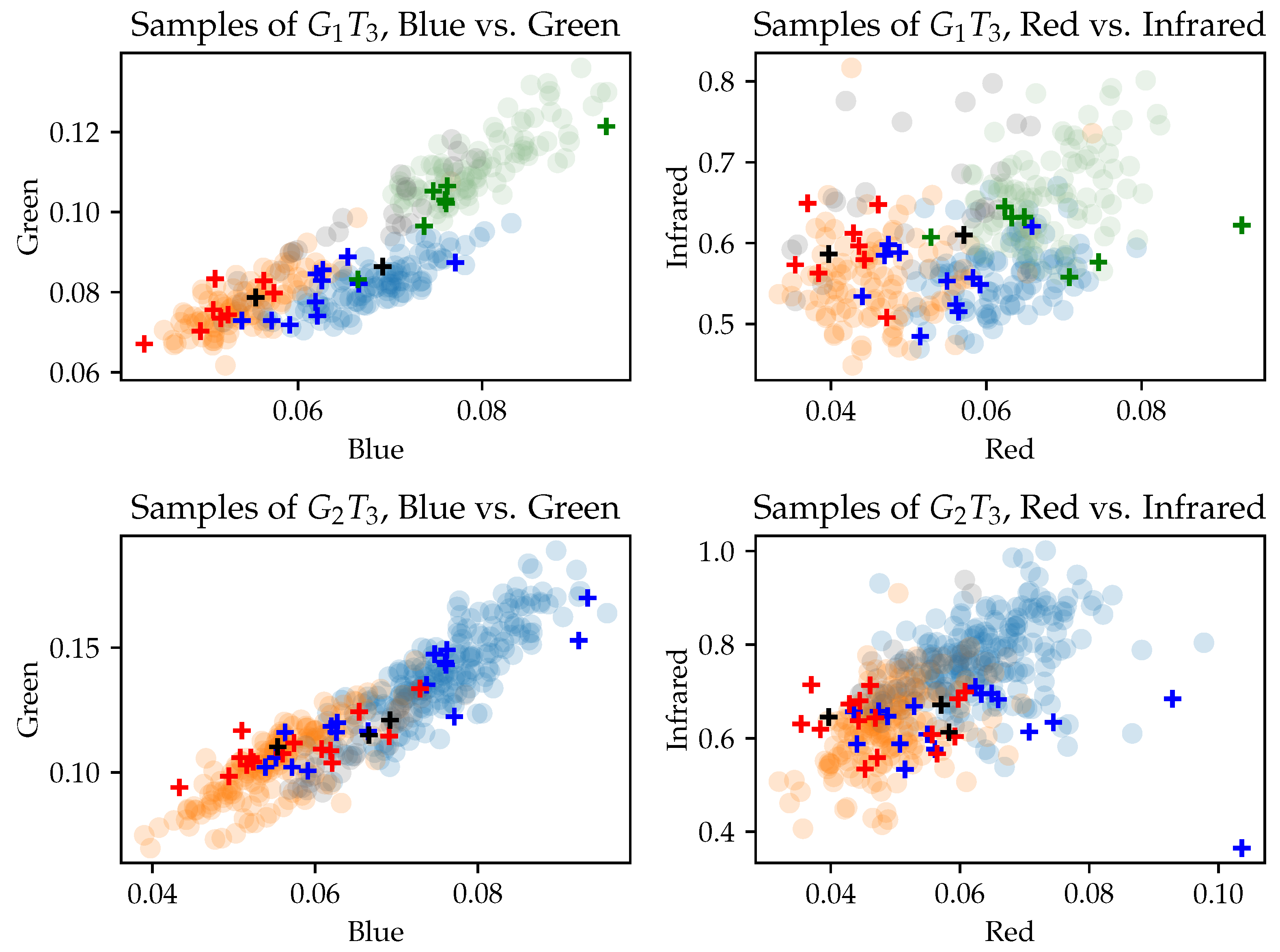
3.3. Separability of Training Data

The mean values for training set and plot samples for $G_1{T}_3$ and $G_2{T}_3$ in blue vs. green and red vs. infrared band combinations were shown in Figure 3.

The samples of the VUs formed clusters which partially overlap. In particular, the spectral samples of the Rumex obtusifolius plants could not be well separated. In blue vs. green band combinations, the clusters were better separated than in the red vs. infrared combination. It was noticeable that the spectral values of the Lolium perenne-community and the Alopecurus pratensis-community show higher variance and mean values at $G_2{T}_3$ than at $G_1{T}_3$. Furthermore, the samples at date $G_2{T}_3$ showed a higher reflectance in the green and infrared band than the samples at $G_1{T}_3$. This was caused by the prominent flower aspect of the grasses at $G_1{T}_3$.

3.4. Classification Results

In

Table 3. Precision, recall, and overall accuracy (OA) (in %) for dependent and independent test data of the four vegetation classifications for Rumex obtusifolium plants, the Lolium perenne-, Alopecurus pratensis-, and Bromus hordeaceus-community and overall accuracy for the object identification (OI).

	Precision in %								OA
	Rumex obtusifolius plants		Lolium perenne-community		Alopecurus pratensis-community		Bromus hordeaceus-community
$G_1{T}_3$	87.72	100	97.98	81.81	99.00	80.00	96.51	83.33	97.06	82.75
$G_2{T}_3$	96.25	33.33	95.51	78.95	97.11	81.82			96.01	71.43
$G_1$	83.33	0.00	93.94	72.73	95.81	70.00	87.34	83.33	91.14	68.97
$G_2$	96.62	100	95.12	94.11	97.68	86.67			95.72	88.57
	Recall in %
$G_1{T}_3$	98.04	71.42	96.37	100	94.75	75	98.04	100	97.06	82.75
$G_2{T}_3$	95.06	33.33	97.50	78.95	94.39	69.23			96.01	71.43
$G_1$	79.71	0.00	96.44	100	83.40	58.33	99.07	71.43	91.14	68.97
$G_2$	98.85	66.67	97.82	84.21	92.32	100			95.72	88.57
$OI$									97.71

, a summary of the validation of the monotemporal VU classification ($G_1{T}_3$ and $G_2{T}_3$), the multitemporal VU classification ($G_1$ and $G_2$) and the object identification ($OI$) can be found. All five classification models reached overall accuracies $>91\%$ on the dependent test data. On the independent test data, the overall accuracy of the VU classifications reached from 68% to 88%. On both the dependent and independent test data, the multitemporal classification of $G_1$ got the lowest overall accuracy. In this, worse accuracies appeared for the classification of Rumex obtusifolius (precision and recall of 0%) and the Alopecurus pratensis-community (precision: 70%, recall: 58.33%).

The result maps of the classifications for $G_1$ and $G_2$ are shown in Figure 4. Both the monotemporal and the multitemporal classifications highlight similar spatial vegetation patterns. In both dates, the transition ranges between VUs were smaller in the multitemporal classification. In the multitemporal classification of $G_1$, more homogeneous areas could be found than in the monotemporal classification. In $G_2$, the results show strong similarities, but differ mainly at the western edge. Subsets of a Rumex obtusifolius-dominated area of the classification results are depicted in Figure 4. Rumex obtusifolius was mainly recognized in the multitemporal classification result of $G_2$. The areas eliminated by the object identification appear as white areas in the results of the monotemporal classifications. In $G_1{T}_3$, especially the area of open ground in the center of the subset was not classified. In $G_2{T}_3$, individual molehills were not included in the classification. In the multitemporal classification, these areas were assigned to the surrounding VUs.

4. Discussion

4.1. Usability of the Presented Methodology in an Agricultural Context

To estimate the forage value of the mown plant material, it is useful to know its species composition [42]. Since this varies spatially, a map is useful for yield estimation. However, it must be considered that the identified plant communities are not static in their composition and vary spatially and temporally [17]. The EIV of the VUs helps to understand the characteristics of an area and to identify potentially more humid, acidic, or nutrient-rich areas. Based on the EIV, few differences can be deduced, both for different observation dates and between the three communities of Alopecurus pratensis, Lolium perenne, and Bromus hordeaceus (see Appendix B). For assessment of forage quality, it is also helpful to estimate the forage value of a VU (see Appendix B), and spatially identify weeds [55]. The species Bromus hordeaceus and Rumex obtusifolius mentioned here as weeds are characterized by a low forage value. As can be seen in Appendix A, Bromus hordeaceus is represented over the entire area in $G_1$. Bromus hordeaceus is a perennial, self-seeding grass that is found primarily in patchy rich pastures [56]. If it exceeds 10% of the vegetation, it can be considered a weed [55]. The areas dominated by Bromus hordeaceus during $G_1$ were classified as Alopecurus pratensis-community in $G_2$.

Rumex obtusifolius occurs as a nitrogen and intensification indicator, as can be seen by N = 9, but due to its high content of oxalic acids and tannins, it is not fed fresh or in hay [42]. Due to its high seed potential, even a single plant should be controlled [55,57]. However, the occurrence of individual grass species that may be harmful to horses is only partially demonstrated by monitoring plant communities. The abundance of individual species within the plant community varies, possibly occurring only in sub-areas. To cover this issue, a classification of more detailed vegetation units is necessary.

4.2. Comparison of Mono- and Multitemporal Data for Plant Community Mapping

In comparison of the mono- and multitemporal VU classification, it was noticeable that larger homogeneous areas are found in both multitemporal classifications. Furthermore, class boundaries could be better delimited in the multitemporal results, and the transition areas were smaller. This could be explained by the expanded feature space of the multitemporal training data. As described in Section 3.2, both the flowering aspect and the occurrence of individual species changed with the phenological phases. It could therefore be assumed that the flowering aspect and the change in vegetation structure had a positive influence on the multitemporal classification, as they should vary the same or similar within a plant community over the vegetation period. However, the validation showed that the monotemporal model for $G_1$ had a higher accuracy on the independent plot data (82.75% to 68.97%, Table 3). For $G_2$, the multitemporal model had a higher accuracy on the independent plot data (88.57% to 71.43%, Table 3).

The authors of [23] showed an improvement of 5–10% in the accuracy of the classification of vegetation functional groups by using multitemporal data. The influence of shadows and flowering was reduced when using data of different phenological stages. In our work, this improvement was only visible in the validation of independent plot data of $G_2$, but in general, the multitemporal models showed a weaker overall accuracy than the monotemporal models. It is possible that the multitemporal models could be improved with extended training data. These models have more input neurons than the monotemporal models and therefore need more data to properly learn the relevant features. The classifier of the multitemporal classification of $G_1$ showed problems, especially in the detection of Rumex obtusifolius. This plant is small and barely detectable at early observation dates of $G_1$ and later overgrown by tall grass, whereas it was present in $G_2$ from the beginning of the observation. The multitemporal classification of $G_1$ showed problems in the detection of the Alopecurus pratensis-community. At early dates, this class was dominated by Alopecurus pratensis, but at later dates the flowering of Holcus lanatus was also visible, especially in the transition areas to the other plant communities. Possibly, these plants caused a decreased accuracy in the multitemporal classification because the borders of the plant communities were less clear at $G_1{T}_3$. Some plots in the northwest of the study site lay in the transition area between the Lolium perenne- and the Alopecurus pratensis-community, which influences the separability.

Object identification showed good results in the monotemporal models (97.72% accuracy, Table 3). In the multitemporal models it was not necessary, because most objects (e.g., molehills) were not temporally stable. Areas that were not classified in the monotemporal models are replaced by the surrounding VU in the multitemporal models (see subfigures of Figure 4). So, areas removed by the object identification did not affect the applicability and interpretability of the result map.

4.3. CNNs for Plant Community Classification in Grasslands

The spectral classes of the VUs could not be separated linearly. Although there were correlations between class membership and spectral information (see Figure 3), these were not sufficient for a separation. The samples of Rumex obtusifolius extended across the other VUs and had no distinctive spectral signature. However, due to their size and structure in rosettes [55], they could be easily distinguished from the surrounding grasses and herbs. The detection of Rumex obtusifolius in grasslands with CNNs was already shown by [32]; the authors achieved an accuracy of over 91% on a monotemporal model. The accuracy of the identification of Rumex obtusifolius with the models presented here varies. The multitemporal model for $G_1$ achieved the worst accuracy with 79.71% on the test set (0% on the plot data). The best accuracy was achieved by the monotemporal model of $G_1$ with 98.04% on the test set (100% on the plot data). The other classes are characterized not only by different spectral values but also by a distinctive spatial structure. The Alopecurus pratensis community is dominated by tall grasses, which are no longer upright because of wind at later observation dates. Thus, a wavy structure becomes visible, which is less apparent in the Lolium perenne-community, where mainly herbs and low grasses are found (see Appendix A).

It was shown by other studies [34,35] that CNNs are suitable for the classification of different plant communities. In this work, individual plants of the species Rumex obtusifolius were identified in addition to the Lolium perenne-, Alopecurus pratensis-, and Bromus hordeaceus-community. Different requirements for classifications of VUs show the great potential of CNNs. A single network can infer and combine multiple spatial and spectral nonlinear features. In this complex problem, good accuracies in separating multiple plant communities and individual plants could be achieved. Even though only a single study site was observed in two growing periods within this study, it can be assumed that the presented methodology can be used in other grasslands with different or differently separated plant communities. For this, a database should be created from grasslands in various expressions at the same or similar phenological phases. With this database, plant communities in various grasslands could be classified with little effort and no deep ecological and botanical knowledge.

5. Conclusions

This work presents a method for the detection of plant communities in grasslands based on CNNs and UAV data. For this, UAV imagery and botanical data were collected at regular intervals in a hay meadow during two growths. Four VUs, a Alopecurus pratensis-community, a Lolium perenne-community, a Bromus hordeaceus-community, and Rumex obtusifolius plants were identified and classified with CNNs. It was investigated whether a multitemporal classification offers added value compared to a monotemporal classification. However, it was shown that not all models trained for this purpose achieved the same accuracy and the classification quality was influenced by phenology. For the preparation of phytosociological relevés, expert knowledge is essential. This complicates the generation of suitable training data for the presented models. Furthermore, only one study site with two different plant communities and two weed species was observed. To transfer the presented methodology to other grasslands to estimate the composition of the vegetation and thus the forage quality, a database of additional grassland plant communities in different variants at the same phenological phase would be necessary. The monotemporal model can give a good impression of the spatial distribution of the different plant communities from a single observation. It should further be investigated whether the accuracy of the multitemporal model can be improved with additional training data.

References

1. Dengler, J.; Tischew, S. Grasslands of Western and Northern Europe—Between intensification and abandonment. In Grasslands of the World: Diversity, Management and Conservation; Squires, V.S., Dengler, J., Hua, L., Feng, H., Eds.; CRC Press: Boca Raton, FL, USA, 2018. [Google Scholar]
2. Leuschner, C.; Ellenberg, H. Ecology of Central European Non-Forest Vegetation: Coastal to Alpine, Natural to Man-Made Habitats: Vegetation Ecology of Central Europe; Springer: Berlin/Heidelberg, Germany, 2018; Volume II. [Google Scholar]
3. Plantureux, S.; Peeters, A.; McCracken, D. Biodiversity in intensive grasslands: Effect of management, improvement and challenges. Agron. Res. 2005, 3, 153–164. [Google Scholar]
4. Wesche, K.; Krause, B.; Culmsee, H.; Leuschner, C. Fifty years of change in Central European grassland vegetation: Large losses in species richness and animal-pollinated plants. Biol. Conserv. 2012, 150, 76–85. [Google Scholar] [CrossRef]
5. European Parliament and the Council. OJ L 347/608; Regulation (EU) No 1307/2013 of the European Parliament and of the Council of 17 December 2013 Establishing Rules for Direct Payments to Farmers Under Support Schemes Within the Framework of the Common Agricultural Policy and Repealing Council Regulation (EC) No 637/2008 and Council Regulation (EC) No 73/2009; European Parliament and the Council: Brussels, Belgium, 2013. [Google Scholar]
6. Niedersächsisches Ministerium für Ernährung, Landwirtschaft und Verbraucherschutz (ML). Merkblatt zu den Besonderen Förderbestimmungen GL 1—Extensive Bewirtschaftung von Dauergrünland GL 11—Grundförderung. Available online: https://www.ml.niedersachsen.de/download/85100/GL_12_-_Merkblatt_Zusatzfoerderung_nicht_vollstaendig_barrierefrei_.pdf (accessed on 7 October 2021).
7. Johansen, M.; Lund, P.; Weisbjerg, M. Feed intake and milk production in dairy cows fed different grass and legume species: A meta-analysis. Animal 2018, 12, 66–75. [Google Scholar] [CrossRef] [PubMed]
8. Sturm, P.; Zehm, A.; Baumbauch, H.; von Brackel, W.; Verbücheln, G.; Stock, M.; Zimmermann, F. Grünlandtypen; Quelle & Meyer Verlag: Wiebelsheim, Germany, 2018. [Google Scholar]
9. Gräßler, J.; von Borstel, U. Fructan content in pasture grasses. Pferdeheilkunde 2005, 21, 75. [Google Scholar] [CrossRef] [Green Version]
10. van Eps, A.; Pollitt, C. Equine laminitis induced with oligofructose. Equine Vet. J. 2006, 38, 203–208. [Google Scholar] [CrossRef] [PubMed]
11. Malinowski, D.; Belesky, D.; Lewis, G. Abiotic stresses in endophytic grasses. In Neotyphodium in Cool-Season Grasses; Blackwell Publishing: Hoboken, NJ, USA, 2005. [Google Scholar] [CrossRef]
12. Bourke, C.A.; Hunt, E.; Watson, R. Fescue-associated oedema of horses grazing on endophyte-inoculated tall fescue grass (Festuca arundinacea) pastures. Aust. Vet. J. 2009, 87, 492–498. [Google Scholar] [CrossRef] [PubMed]
13. Bengtsson, J.; Bullock, J.M.; Egoh, B.; Everson, C.; Everson, T.; O’Connor, T.; O’Farrell, P.; Smith, H.; Lindborg, R. Grasslands—More important for ecosystem services than you might think. Ecosphere 2019, 10, e02582. [Google Scholar] [CrossRef]
14. Le Clec’h, S.; Finger, R.; Buchmann, N.; Gosal, A.S.; Hörtnagl, L.; Huguenin-Elie, O.; Jeanneret, P.; Lüscher, A.; Schneider, M.K.; Huber, R. Assessment of spatial variability of multiple ecosystem services in grasslands of different intensities. J. Environ. Manag. 2019, 251, 109372. [Google Scholar] [CrossRef]
15. Lavorel, S.; Grigulis, K.; Lamarque, P.; Colace, M.P.; Garden, D.; Girel, J.; Pellet, G.; Douzet, R. Using plant functional traits to understand the landscape distribution of multiple ecosystem services. J. Ecol. 2011, 99, 135–147. [Google Scholar] [CrossRef]
16. Díaz, S.; Lavorel, S.; de Bello, F.; Quétier, F.; Grigulis, K.; Robson, T.M. Incorporating plant functional diversity effects in ecosystem service assessments. Proc. Natl. Acad. Sci. USA 2007, 104, 20684–20689. [Google Scholar] [CrossRef] [Green Version]
17. Smith, T.; Huston, M. A theory of the spatial and temporal dynamics of plant communities. In Progress in Theoretical Vegetation Science; Springer: Berlin/Heidelberg, Germany, 1990; pp. 49–69. [Google Scholar] [CrossRef]
18. Dierschke, H. Pflanzensoziologie: Grundlagen und Methoden; 55 Tabellen; Eugen Ulmer KG: Darmstadt, Germany, 1994. [Google Scholar]
19. Mueller-Dombois, D.; Ellenberg, H. Aims and Methods of Vegetation Ecology; The Blackburn Press: West Caldwell, NJ, USA, 2003. [Google Scholar]
20. Zlinszky, A.; Schroiff, A.; Kania, A.; Deák, B.; Mücke, W.; Vári, Á.; Székely, B.; Pfeifer, N. Categorizing grassland vegetation with full-waveform airborne laser scanning: A feasibility study for detecting Natura 2000 habitat types. Remote Sens. 2014, 6, 8056–8087. [Google Scholar] [CrossRef] [Green Version]
21. Reinermann, S.; Asam, S.; Kuenzer, C. Remote sensing of grassland production and management—A review. Remote Sens. 2020, 12, 1949. [Google Scholar] [CrossRef]
22. Kattenborn, T.; Leitloff, J.; Schiefer, F.; Hinz, S. Review on Convolutional Neural Networks (CNN) in vegetation remote sensing. ISPRS J. Photogramm. Remote Sens. 2021, 173, 24–49. [Google Scholar] [CrossRef]
23. Wood, D.J.; Preston, T.M.; Powell, S.; Stoy, P.C. Multiple UAV Flights across the Growing Season Can Characterize Fine Scale Phenological Heterogeneity within and among Vegetation Functional Groups. Remote Sens. 2022, 14, 1290. [Google Scholar] [CrossRef]
24. Rapinel, S.; Mony, C.; Lecoq, L.; Clement, B.; Thomas, A.; Hubert-Moy, L. Evaluation of Sentinel-2 time-series for mapping floodplain grassland plant communities. Remote Sens. Environ. 2019, 223, 115–129. [Google Scholar] [CrossRef]
25. Fauvel, M.; Lopes, M.; Dubo, T.; Rivers-Moore, J.; Frison, P.L.; Gross, N.; Ouin, A. Prediction of plant diversity in grasslands using Sentinel-1 and-2 satellite image time series. Remote Sens. Environ. 2020, 237, 111536. [Google Scholar] [CrossRef]
26. Cruzan, M.B.; Weinstein, B.G.; Grasty, M.R.; Kohrn, B.F.; Hendrickson, E.C.; Arredondo, T.M.; Thompson, P.G. Small unmanned aerial vehicles (micro-UAVs, drones) in plant ecology. Appl. Plant Sci. 2016, 4, 1600041. [Google Scholar] [CrossRef]
27. Gholizadeh, H.; Gamon, J.A.; Townsend, P.A.; Zygielbaum, A.I.; Helzer, C.J.; Hmimina, G.Y.; Yu, R.; Moore, R.M.; Schweiger, A.K.; Cavender-Bares, J. Detecting prairie biodiversity with airborne remote sensing. Remote Sens. Environ. 2019, 221, 38–49. [Google Scholar] [CrossRef]
28. Lu, B.; He, Y. Species classification using Unmanned Aerial Vehicle (UAV)-acquired high spatial resolution imagery in a heterogeneous grassland. ISPRS J. Photogramm. Remote Sens. 2017, 128, 73–85. [Google Scholar] [CrossRef]
29. Weisberg, P.J.; Dilts, T.E.; Greenberg, J.A.; Johnson, K.N.; Pai, H.; Sladek, C.; Kratt, C.; Tyler, S.W.; Ready, A. Phenology-based classification of invasive annual grasses to the species level. Remote Sens. Environ. 2021, 263, 112568. [Google Scholar] [CrossRef]
30. Wijesingha, J.; Astor, T.; Schulze-Brüninghoff, D.; Wengert, M.; Wachendorf, M. Predicting forage quality of grasslands using UAV-borne imaging spectroscopy. Remote Sens. 2020, 12, 126. [Google Scholar] [CrossRef] [Green Version]
31. Pecina, M.V.; Bergamo, T.F.; Ward, R.; Joyce, C.; Sepp, K. A novel UAV-based approach for biomass prediction and grassland structure assessment in coastal meadows. Ecol. Indic. 2021, 122, 107227. [Google Scholar] [CrossRef]
32. Valente, J.; Doldersum, M.; Roers, C.; Kooistra, L. Detecting Rumex Obtusifolius weed plants in grasslands from UAV RGB imagery using deep learning. ISPRS Ann. Photogramm. Remote Sens. Spat. Inf. Sci. 2019, 4, 179–185. [Google Scholar] [CrossRef] [Green Version]
33. Lam, O.H.Y.; Dogotari, M.; Prüm, M.; Vithlani, H.N.; Roers, C.; Melville, B.; Zimmer, F.; Becker, R. An open source workflow for weed mapping in native grassland using unmanned aerial vehicle: Using Rumex obtusifolius as a case study. Eur. J. Remote Sens. 2021, 54, 71–88. [Google Scholar] [CrossRef]
34. Kattenborn, T.; Eichel, J.; Fassnacht, F.E. Convolutional Neural Networks enable efficient, accurate and fine-grained segmentation of plant species and communities from high-resolution UAV imagery. Sci. Rep. 2019, 9, 17656. [Google Scholar] [CrossRef] [PubMed] [Green Version]
35. Kattenborn, T.; Eichel, J.; Wiser, S.; Burrows, L.; Fassnacht, F.E.; Schmidtlein, S. Convolutional Neural Networks accurately predict cover fractions of plant species and communities in Unmanned Aerial Vehicle imagery. Remote Sens. Ecol. Conserv. 2020, 6, 472–486. [Google Scholar] [CrossRef] [Green Version]
36. Zhu, X.X.; Tuia, D.; Mou, L.; Xia, G.S.; Zhang, L.; Xu, F.; Fraundorfer, F. Deep learning in remote sensing: A comprehensive review and list of resources. IEEE Geosci. Remote Sens. Mag. 2017, 5, 8–36. [Google Scholar] [CrossRef] [Green Version]
37. Niedersächsisches Landesamt für Bergbau, Energie und Geologie (LBEG). Bodenübersichtskarte im Maßstab 1:50 000 (BÜK50); LBEG: Hannover, Germany, 1999. [Google Scholar]
38. Meteostat. Belm. Available online: https://meteostat.net/en/station/D0342 (accessed on 7 October 2021).
39. Reichelt, G.; Wilmanns, O. Vegetationsgeographie; Westermann: Braunschweig, Germany, 1973. [Google Scholar]
40. Jäger, E.J. Rothmaler-Exkursionsflora von Deutschland. Gefäßpflanzen: Grundband, 21st ed.; Springer-Verlag: Berlin/Heidelberg, Germany, 2017. [Google Scholar]
41. Ellenberg, H.; Weber, H.E.; Düll, R.; Wirth, V.; Werner, W.; Paulißen, D. Zeigerwerte von Pflanzen in Mitteleuropa, 3, durch gesehene Aufl. Scr. Geobot. 2001, 18, 1–261. [Google Scholar]
42. Dierschke, H.; Briemle, G. Kulturgrasland, 2nd ed.; Eugen Ulmer KG: Darmstadt, Germany, 2008. [Google Scholar]
43. Shorten, C.; Khoshgoftaar, T.M. A survey on image data augmentation for deep learning. J. Big Data 2019, 6, 1–48. [Google Scholar] [CrossRef]
44. Pawara, P.; Okafor, E.; Schomaker, L.; Wiering, M. Data augmentation for plant classification. In Proceedings of the International Conference on Advanced Concepts for Intelligent Vision Systems, Antwerp, Belgium, 18–21 September 2017; pp. 615–626. [Google Scholar] [CrossRef]
45. LeCun, Y.; Boser, B.E.; Denker, J.S.; Henderson, D.; Howard, R.E.; Hubbard, W.E.; Jackel, L.D. Handwritten digit recognition with a back-propagation network. In Proceedings of the Advances in Neural Information Processing Systems, Denver, CO, USA, 26–29 November 1990; pp. 396–404. [Google Scholar]
46. LeCun, Y.; Bengio, Y.; Hinton, G. Deep learning. Nature 2015, 521, 436–444. [Google Scholar] [CrossRef]
47. Rawat, W.; Wang, Z. Deep convolutional neural networks for image classification: A comprehensive review. Neural Comput. 2017, 29, 2352–2449. [Google Scholar] [CrossRef] [PubMed]
48. Springenberg, J.T.; Dosovitskiy, A.; Brox, T.; Riedmiller, M. Striving for simplicity: The all convolutional net. arXiv 2014, arXiv:1412.6806. [Google Scholar] [CrossRef]
49. He, K.; Zhang, X.; Ren, S.; Sun, J. Deep residual learning for image recognition. In Proceedings of the IEEE Conference on Computer Vision and Pattern Recognition, Las Vegas, NV, USA, 27–30 June 2016; pp. 770–778. [Google Scholar] [CrossRef]
50. Zhang, Z.; Sabuncu, M. Generalized cross entropy loss for training deep neural networks with noisy labels. Adv. Neural Inf. Process. Syst. 2018, 31, 8778–8788. [Google Scholar]
51. Kingma, D.P.; Ba, J. Adam: A method for stochastic optimization. arXiv 2014, arXiv:1412.6980. [Google Scholar] [CrossRef]
52. Thakkar, V.; Tewary, S.; Chakraborty, C. Batch Normalization in Convolutional Neural Networks—A comparative study with CIFAR-10 data. In Proceedings of the 2018 5th International Conference on Emerging Applications of Information Technology (EAIT), West Bengal, India, 12–13 January 2018; pp. 1–5. [Google Scholar] [CrossRef]
53. Phaisangittisagul, E. An analysis of the regularization between L2 and dropout in single hidden layer neural network. In Proceedings of the 2016 7th International Conference on Intelligent Systems, Modelling and Simulation (ISMS), Bangkok, Thailand, 25–27 January 2016; pp. 174–179. [Google Scholar] [CrossRef]
54. Sokolova, M.; Lapalme, G. A systematic analysis of performance measures for classification tasks. Inf. Process. Manag. 2009, 45, 427–437. [Google Scholar] [CrossRef]
55. Elsäßer, M.; Engel, S.; Roßberg, R.; Thumm, U. Unkräuter im Grünland. Erkennen - Bewerten - Handeln, 2nd ed.; DLG-Verlag: Frankfurt am Main, Germany, 2018. [Google Scholar]
56. Klapp, E.; Opitz von Boberfeld, W. Taschenbuch der Gräser, 12th ed.; Eugen Ulmer KG: Darmstadt, Germany, 2013. [Google Scholar]
57. Stilmant, D.; Bodson, B.; Vrancken, C.; Losseau, C. Impact of cutting frequency on the vigour of Rumex obtusifolius. Grass Forage Sci. 2010, 65, 147–153. [Google Scholar] [CrossRef]
Figure 1. Location of the study site in Germany (top left) and the district of Osnabrück (bottom left). Orthomosaic and grassland vegetation of one plot of 06/08/2021 (right).
Remotesensing 15 01945 g001
Figure 2. Schematic workflow of preprocessing, training, validation, and classification.
Remotesensing 15 01945 g002
Figure 3. Scatter plots of the samples of the dependent (○) and independent (+) test data in blue vs. green and red vs. infrared. Colors are used as follows: grey: Rumex obtusifolius plants, blue: Lolium perenne-community, red: Alopecurus pratensis-community, green: Bromus Hordeaceus-community.
Remotesensing 15 01945 g003
Figure 4. Subsets of the classification results of the mono- and multitemporal model and orthomosaics in RGB-color of G 1 T 3 and G 2 T 3 .
Remotesensing 15 01945 g004