A 3D Interferometer-Type Lightning Mapping Array for Observation of Winter Lightning in Japan

Abstract

We have developed and deployed a 3D Interferometer-type Lightning Mapping Array (InLMA) for observing winter lightning in Japan. InLMA consists of three broadband interferometers installed at three stations with a distance from 3 to 5 km. At each interferometer station, three discone antennas were installed, forming a right triangle with a separation of 75 m along their two orthogonal baselines. The output of each InLMA antenna is passed through a 400 MHz low-pass filter and then recorded at 1 GS/s with 16-bit accuracy. A new method has been proposed for finding 3D solutions of a lightning mapping system that consists of multiple interferometers. Using the InLMA, we have succeeded in mapping a positive cloud-to-ground (CG) lightning flash in winter, particularly its preliminary breakdown (PB) process. A study on individual PB pulse processes allows us to infer that each PB pulse process contains many small-scale discharges scattering in a height range of about 150 m. These small-scale discharges in a series of PB pulses appear to be continuous in space, though discontinuous in time. We have also examined the positive return stroke in the CG flash and found a 3D average return stroke speed of 7.5 × 10⁷ m/s.

1. Introduction

As demonstrated by Wang et al. [1] and Zheng et al. [2], winter thunderstorms in Japan could exhibit various charge structures featured with low altitudes and small separations between charge regions of opposite polarities. Under such charge structures, many lightning flashes tend to have very complicated characteristics, as shown in a case study by Huang et al. [3]. In order to understand such complicated lightning, it is necessary to track their progressions in both time and space. Recently, we have developed a 3D lightning mapping system called DALMA (Discone Antenna Lightning Mapping Array) [4] for observing the 3D progressions of winter lightning in Japan. DALMA is based on the TOA technique and works at MF-HF bands. As shown by Wang et al. [4], for each of the two examples of lightning flashes, more than three thousand sources are successfully located with the DALMA. However, as is expected, DALMA can only locate pulse discharges with sufficient MF-HF radiations. This significantly limits the time resolution of DALMA. Therefore, many lightning discharge processes, such as preliminary breakdowns and return strokes, cannot be studied in detail with DALMA. To overcome these problems, we have developed and deployed an interferometer-type lightning mapping array in the area covered by DALMA, and we have operated a supplementary system to DALMA for studying detailed lightning discharge processes in a small area.

As reviewed by Stock et al. [5], interferometers have been used in lightning mapping for more than 40 years. Historically, interferometers used narrowband radio signals of lightning through hardware interferometry techniques [6,7], but nowadays almost all interferometers utilize broadband signals through software interferometry approaches pioneered by Shao et al. [8], Ushio et al. [9], Akita et al. [10], and Stock et al. [5]. Recently, 3D interferometers with two stations have been developed and tested [10,11,12,13]. In such systems, 3D mapping is usually achieved using the triangulation method by combining azimuth and elevation angles from the two stations, as detailed by Thyer [14] and Liu et al. [15]. A similar method was used by Mardiana et al. [16]. Recently, Jensen et al. [13] have included timing information for better matching of the azimuth and elevation angles from two stations. The 3D interferometer system developed in this study consists of three stations. For the 3D mapping, instead of using the triangulation method, we have proposed a new method that can be easily used in a system with multiple stations, which, of course, includes the two station systems already reported in the literature [10,11,12,13]. Furthermore, as discussed by Stock et al. [5], the performance of an interferometer is related to many factors, such as noise level, sampling rate, bit number of a digitizer, and baseline length. In order to achieve high performance, we have used a digitizer that operates at 16 bits and has a maximum sampling rate of 1 GHz. The baseline used in this study is 75 m, which is more than twice longer than those used in previous 3D interferometer systems. This paper aims to report the instrumentation, the method, and the preliminary results of our new system.

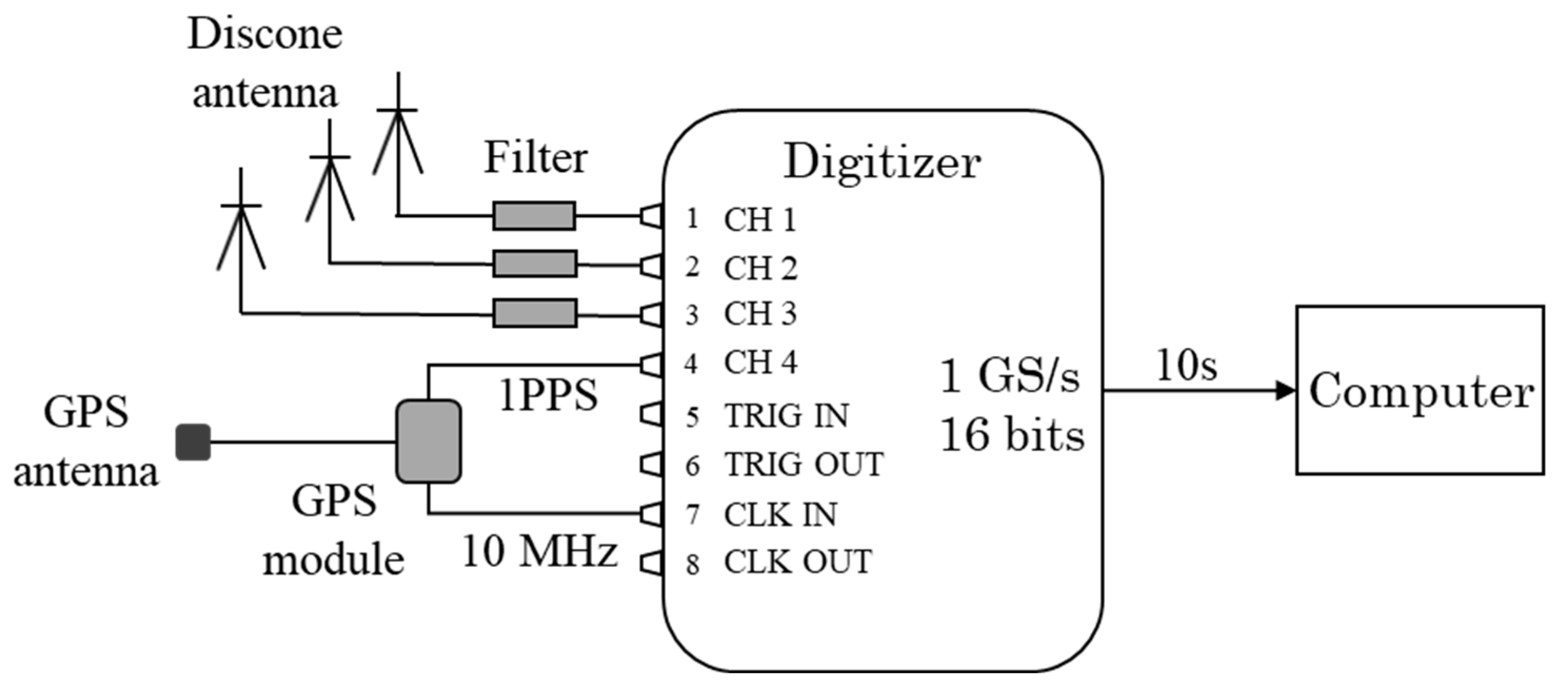
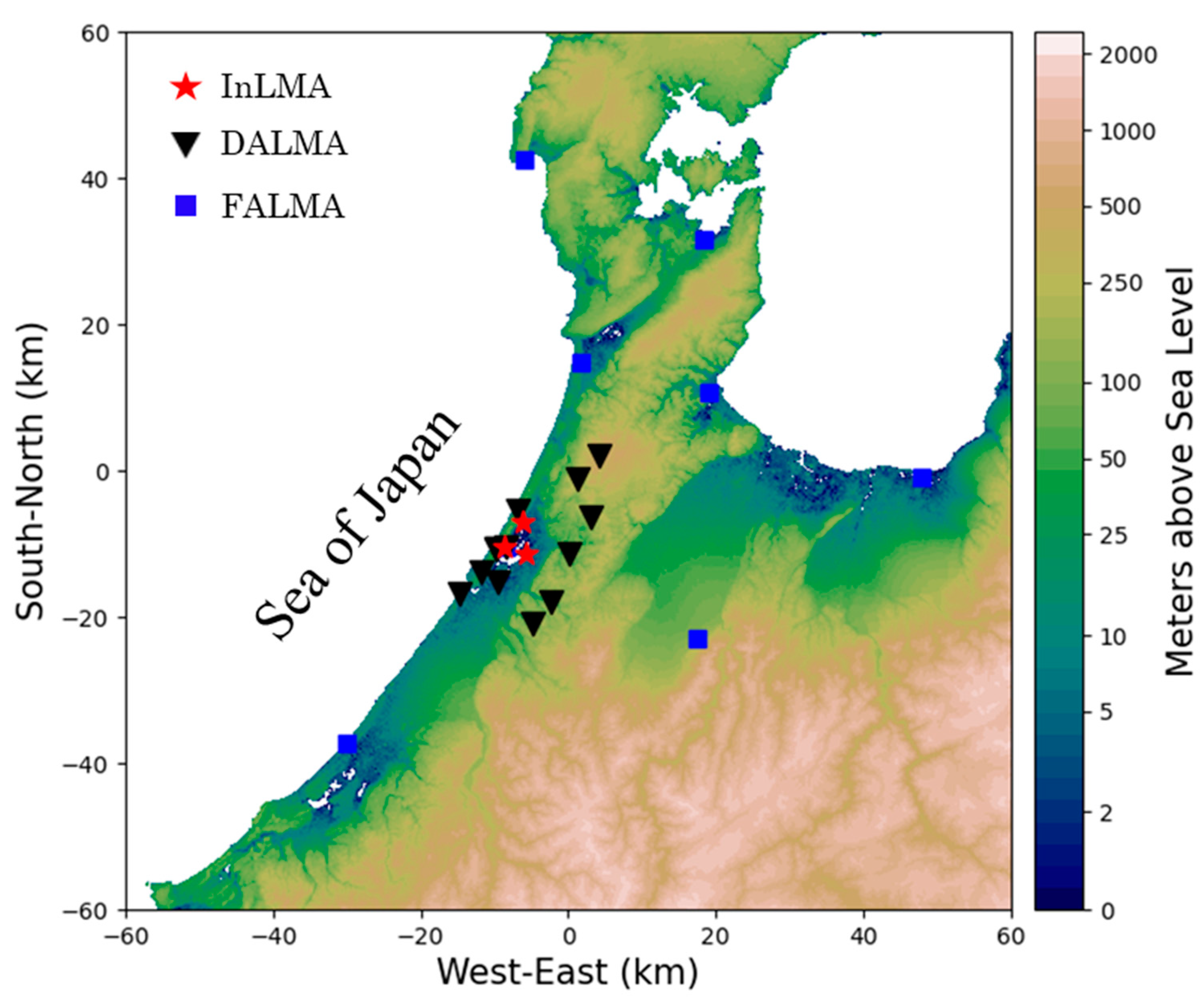
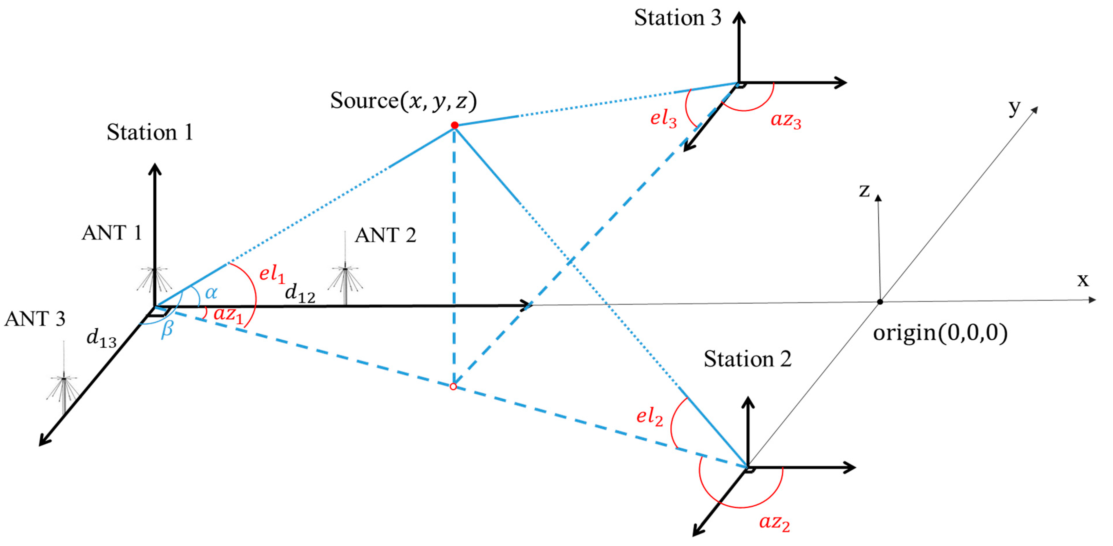
2. Instrumentation and Methods

Figure 1 shows the schematic of the interferometer hardware at one station in this study. The outputs of three discone antennas are connected to three channels of a Gage PCI Express CompuScope digitizer through three 400 MHz low-pass filters, respectively. The 1 PPS output of a GPS receiver named FURY-10M is connected to the 4th channel of the digitizer. The rising edge of this 1 PPS signal is used to synchronize different stations. The digitizer is disciplined using the GPS 10 MHz output, so the synchronization accuracy should be better than 100 ns. We use a compact industrial computer to control the digitizer. The digitizer has a 4 GS/8 GB onboard sample memory. For each trigger, the 4-channel data, each sampled at 1 GHz for 0.8 s, are first recorded on this memory and are then transferred to the hard disk of the computer with a transit time of about 10 s. The digitizer can be operated in pre-trigger mode. However, for every channel, only 8192 sampling points are available for pre-trigger memory. The discone antennas that we used are called Super Discone Antenna D1300AM, which is the same for DALMA, and receives electromagnetic radiation in the frequency range from less than 1 MHz to over 1300 MHz. Three discone antennas were separated at a distance of 75 m, forming a right triangle.

We have equipped 3 identical interferometers at 3 stations separated with a distance of 3–5 km. As a system, these 3 interferometers are called InLMA, short for Interferometer-type Lightning Mapping Array. Figure 2 shows the site map of InLMA. All 3 InLMA stations are set up near a windmill in the Uchinada town of Ishikawa, Japan, where we have been carrying out various lightning observation experiments for more than 17 years [17]. In our recent observations, we also deployed FALMA [18,19] (fast antenna lightning mapping array) and DALMA. FALMA and DALMA sites are also included in Figure 2. FALMA covers a wider area than DALMA, while DALMA covers a wider area than InLMA.

For a signal source whose geometric size is much smaller than its distance to the antennas of InLMA, it can be regarded as a point with its coordinates of $\left(x,y,z\right)$ as shown in Figure 3. We assume that this signal arrives at 3 stations with elevations ${el}_1$, ${el}_2$, and ${el}_3$ and azimuths ${az}_1$, ${az}_2$, and ${az}_3$, respectively. At each station, the azimuth and the elevation can be calculated using the method outlined by M. G. Stock et al. [5], among others [20,21,22]. Let us take station 1 as the example. Assume that the two distances between the antennas (ANT1, ANT2, and ANT3) along the two baselines of station 1 are $d_{12}$ and $d_{13}$, the geometry angles between the signal incident wave and the two baselines are $\alpha$ and $\beta$, and the corresponding time arrival differences of the signal are ${\tau }_{12}$ and ${\tau }_{13}$. In this study, ${\tau }_{12}$ and ${\tau }_{13}$ are obtained using cross correlation between the signals from 2 corresponding antennas, according to the geometric relationship in Figure 3,

$$cos\alpha =\frac{c{\tau }_{12}}{d_{12}}$$

(1)

$$cos\beta =\frac{c{\tau }_{13}}{d_{13}}$$

(2)

where c is the speed of light. According to geometry, cosine $\alpha$ and $\beta$ can be substituted with the azimuth ${az}_1$ and elevation ${el}_1$ of the incident source.

$$cos\alpha =\mathit{cos}\left({az}_1\right)\mathit{cos}\left({el}_1\right),$$

(3)

$$cos\beta =\mathit{sin}\left({az}_1\right)\mathit{cos}\left({el}_1\right),$$

(4)

Combining (1), (2), (3), (4), the azimuth and elevation can be obtained as follows.

$${az}_1=arctan\left(\frac{{\tau }_{12}}{{\tau }_{13}}\right),$$

(5)

$${el}_1=arccos\left(\frac{c}{d}\sqrt{{{\tau }_{12}}^2+{{\tau }_{13}}^2}\right)(\mathrm{i}\mathrm{n} \mathrm{t}\mathrm{h}\mathrm{i}\mathrm{s} \mathrm{s}\mathrm{t}\mathrm{u}\mathrm{d}\mathrm{y} d=d_{12}=d_{13}),$$

(6)

Due to that $\mathit{arctan}\left(x\right)\in \left(-\frac{\pi }{2},\frac{\pi }{2}\right)$ and elevation is limited to positive after being inverted, Equations (5) and (6) cannot include all the possibilities of direction. Consequently, according to the value of $cos\beta$, azimuth should be adjusted sometimes. If $cos\beta <0$°, azimuth should be 180° larger. In this way, for 2D mapping, azimuth is limited to $\left(-\frac{\pi }{2},\frac{3\pi }{2}\right)$ and elevation is limited to $\left(0,\frac{\pi }{2}\right)$.

Similarly, we can also get ${el}_2$, ${az}_2$, and ${el}_3$ and ${az}_3$ for stations 2 and 3. Meanwhile, since all 3 stations are equipped with GPS, we can also get the time differences ${∆t}_{1j}$ between that for a source to arrive at station 1 and the remaining two stations ($j$ = 2, 3).

For a given source $\left(x,y,z\right)$ discharge occurring at time t, according to geometry, we can find its azimuths ${{az}^{\prime }}_i(x,y,z)$ and elevations ${{el}^{\prime }}_i(x,y,z)$ of all stations, as well as the time differences ${∆t^{\prime }}_{1j}(x,y,z)$ between that for a source to arrive at station 1 and the remaining 2 stations ($j$ = 2, 3). In this study, we propose the use of the following ${\chi }^2$ equation to find the best solution of $(x,y,z)$ for the set of the corresponding ${az}_1$, ${el}_1$, ${az}_2$, ${el}_2$, ${az}_3$, ${el}_3$, ${∆t}_{12}$, ${∆t}_{13}$ described above.

$${\chi }^2=\sum _{i=1}^N{[(\frac{{el}_i-{{el}^{\prime }}_i(x,y,z)}{{\sigma }_{el}^i})}^2+{(\frac{{az}_i-{{az}^{\prime }}_i(x,y,z)}{{\sigma }_{az}^i})}^2]+\sum _{j=2}^N{(\frac{{∆t}_{1j}-{∆t^{\prime }}_{1j}(x,y,z)}{{\sigma }_t^i})}^2$$

(7)

where $N$ is the total number of stations ($N=3$ in this study), ${\sigma }_{el}^i, {\sigma }_{az}^i, {\sigma }_t^i$ are random measurement errors of elevation, azimuth, and time, respectively.

The flow chart for realizing 3D location is shown in Figure 4a. First, we divided the data recorded at each channel of the 3 stations into a series of uniform windows based on the GPS PPS signal as the time reference. Secondly, using the window data and cross correlation, we found the time differences between the antennas of each station. Thirdly, from these time differences, we got all the azimuths and elevations. Fourthly, by matching windows of different stations and cross correlation, we found the time differences between different stations. The method for matching the time windows and then finding the time differences between the 2 stations is shown in Figure 4b. The red triangles are used to indicate the same discharge event observed at station 1 and station 2. Apparently, the time difference consists of two parts: ${∆t}_{12}^w$ and ${∆t}_{12}^c$. The first part is the time difference, which can be measured in time windows (window 1 and window 3 in this case), and the second part is the time difference bounded by the time window and can be found by the cross correlation method. Finally, the Least-square method using the ${\chi }^2$ equation in (7) is used not only for finding the best solution of $\left(x,y,z\right)$, but also for matching the windows. If there are any windows used multiple times in previous solutions, only the solution with the smallest ${\chi }^2$ is reserved.

3. Observation and Data

We finished deployment of the InLMA and started the observations of winter lightning in the Hokuriku area of Japan at the end of November of 2021. Since then, more than 100 lightning flashes have been recorded by InLMA. However, during December of 2021, one station of the InLMA was damaged by the voltage surge caused by nearby lightning. Only one of the lightning flashes, which occurred at 20:27:52 on 21 December 2021, was recorded by three stations of InLMA. The electric field change of the lightning flash recorded at one station of FALMA is shown in Figure 5. The “atmospheric electricity” sign convention is used. From the expanded waveforms of the E-field change, we know that it is a positive cloud-to-ground (CG) flash, which consists of two stages of the characteristic PB (preliminary breakdown) pulses (Figure 5b,d,e) and a single positive return stroke (Figure 5c,f). Based on Figure 5f, the peak current of the return stroke is estimated to be about 38 kA [23]. Figure 6 shows its 3D mapping through DALMA. A total of 881 sources were located by DALMA. According to this mapping, the lightning flash started from a height of about 2.4 km MSL at a distance of about 15 km away from the central position of InLMA. The main sources mapped by DALMA occurred in the first 150 ms, which agrees with the waveform shown in Figure 5. An initial negative leader was observed to propagate upward and then divide into two main parts. The return stroke happened about 62.6 ms after lightning initiation. As shown in Figure 6, the lightning discharge sources spread into an area with a horizontal scale of several tens of kilometers, while only a few sources appeared above InLMA.

An example waveform of the corresponding raw data of InLMA along with the spectrums of the main lightning signal and background noise, separately denoted, is shown in Figure 7. The lightning signal mainly appears in the first 150 ms with a frequency bandwidth from about 1 MHz to more than 300 MHz. Previously, we have tried various frequency bands for the mapping and found some small differences in the mapping results [24], but in this study, we only use the frequency band from 80 MHz to 230 MHz.

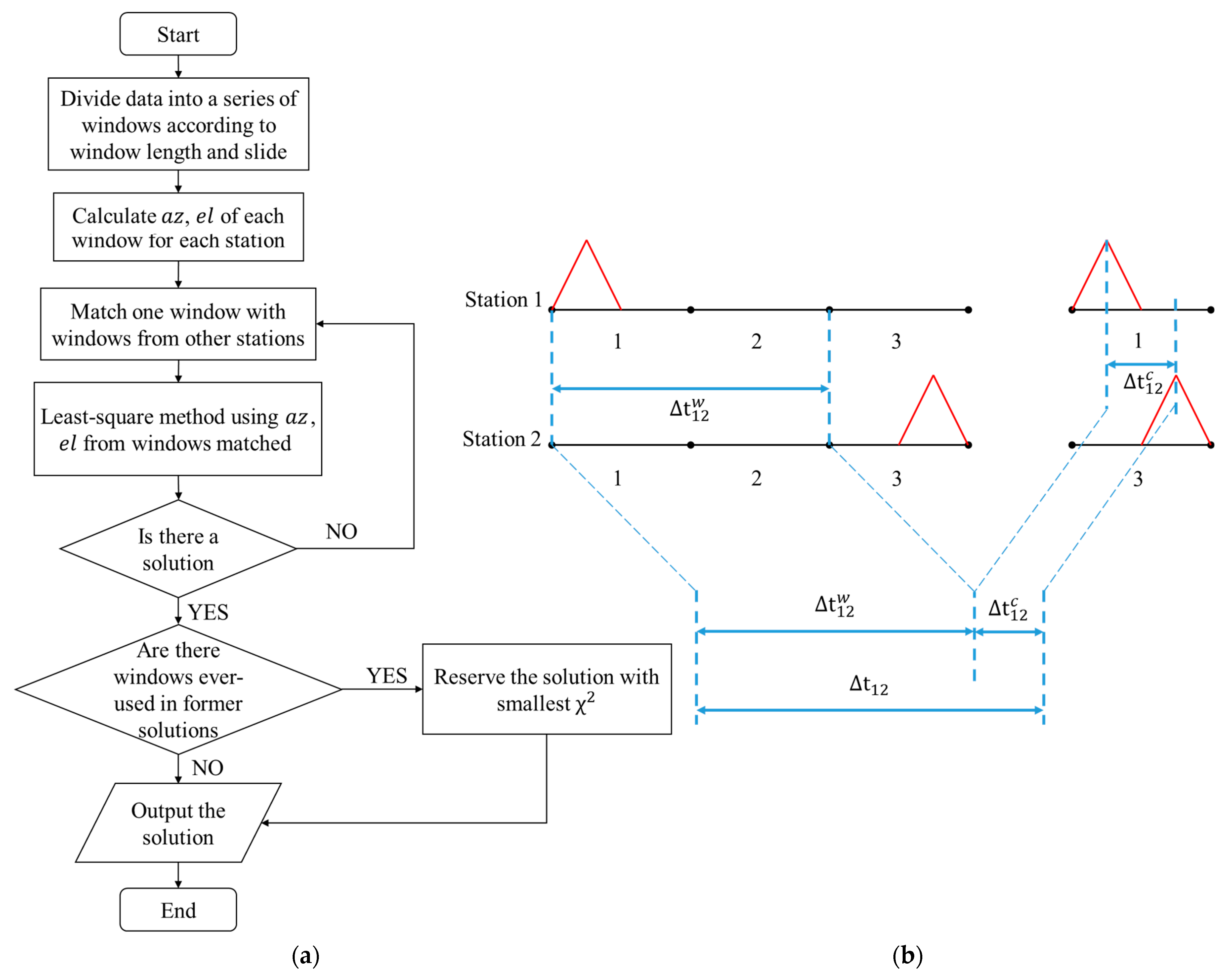
4. Preliminary Results

When performing cross correlation to find the time difference between the different antennas of an InLMA station or different stations, there is a need to choose the proper length of the window and the sliding step. In this study, 1024 sampling points were chosen for the window and 256 sampling points were chosen for the sliding step after trial and error. When solving the ${\chi }^2$ equation, the random measurement errors of elevation and azimuth ${\sigma }_{el}^i, {\sigma }_{az}^i$ are chosen as one degree, based on our previous study using upward lightning data [24]. The error of ${\sigma }_t^i$ is chosen as 100 ns limited by the time accuracy of the GPS 1PPS signal.

4.1. 2D Mapping Using Individual Stations

In order to demonstrate the basic functions of our system, we start by showing 2D mapping results from one station of InLMA in Figure 8 with (a) azimuth versus time, (b) elevation versus time, and (c) azimuth versus elevation for the initial 20 ms processes of the flash. The time is color-coded. In addition, Figure 8a shows the waveform of the corresponding VHF signal recorded by InLMA after being filtered into bandwidth from 80 MHz to 230 MHz. This bandwidth is used for all the mapping of InLMA in this study, as described above. The simultaneous E-field change waveform recorded by FALMA is shown in Figure 8b. As shown in Figure 8c, this flash started from an elevation of about 10° with a negative leader moving upward. After propagating about 0.4 ms, the leader divided into two branches. Branch 1 continues to move upward and branch 2 propagates horizontally to the left. The first preliminary breakdown apparently occurred along Branch 1 and the second preliminary breakdown occurred along branch 2. The preliminary breakdown process should be an indicator of a strong electric field region. Therefore, this lightning flash initially appears to involve two regions of strong electric fields with their vectors in completely different directions. This result again indicates the complicated nature of the charge structure of winter thunderstorms.

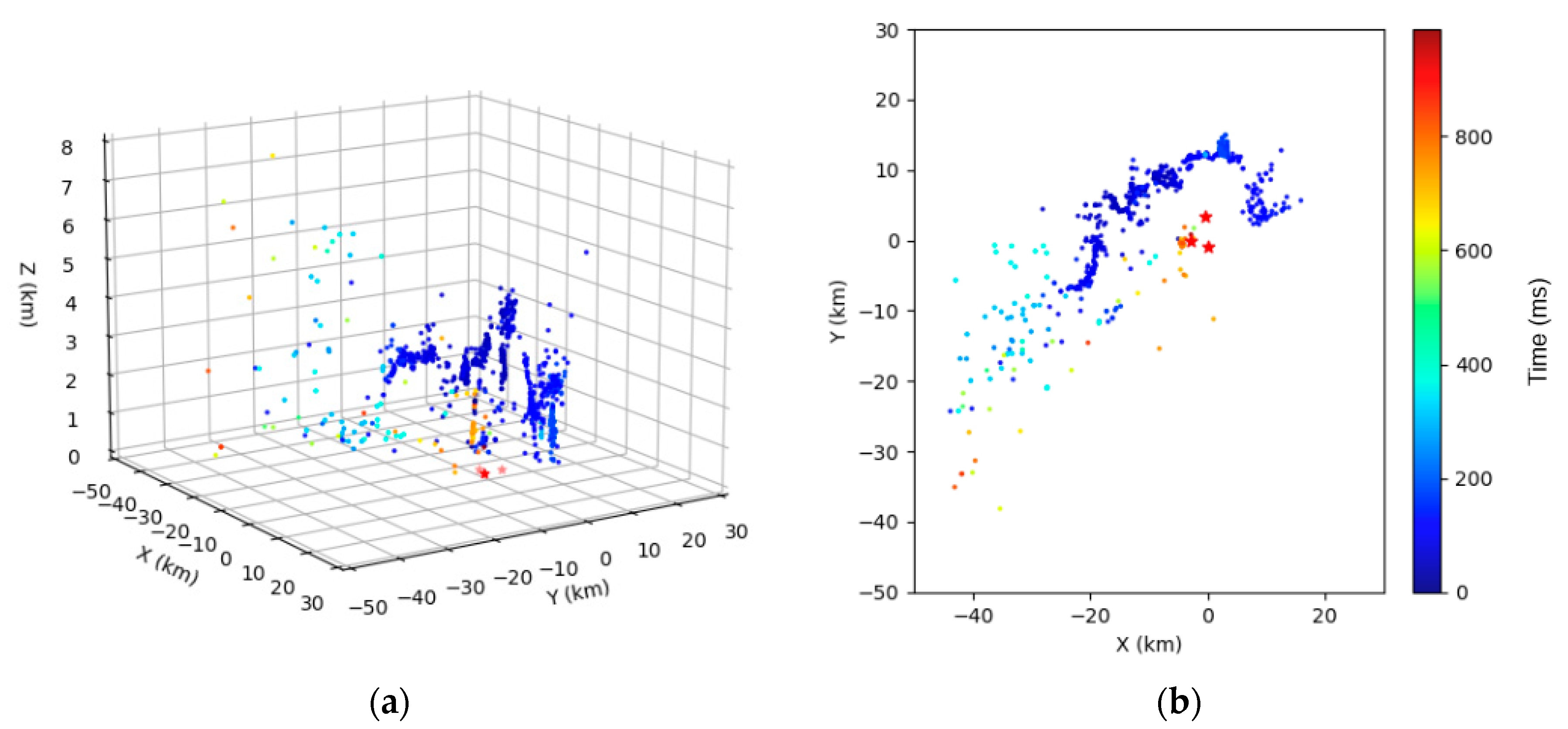
4.2. 3D Mapping by Using 3 Stations

Figure 9 compares the 3D mappings of InLMA and DALMA for the initial 10 ms of the flash with the (a) InLMA mapping result and (b) DALMA mapping result. Time is color-coded. Three red pentagrams represent the three stations of InLMA. Generally, InLMA and DALMA show consistent mapping results. InLMA mapped 1266 sources, while DALMA only mapped 119 sources. Clearly, as expected, InLMA has shown a more detailed progression of processes. The average speeds of branch 1 and branch 2 are about 1.5 × 10⁶ m/s and 1.4 × 10⁶ m/s, respectively. Figure 10 compares the source heights mapped by InLMA and DALMA. It appears that the DALMA-mapped sources of the first preliminary breakdown tend to have a lower height than those mapped by InLMA. Since the first PB is moving in an upward direction, this result may indicate that a PB discharge event involves many small-scale discharge events, as detected by InLMA, and a big scale event at the bottom that radiates lower frequency radio waves, as detected by DALMA. Additionally, the discharge channel mapped by DALMA is much thinner than those mapped by InLMA. It appears that a PB process may involve many small branches that have been mapped by InLMA, but not by DALMA. Interestingly, during the very initial stage, there is a small branch that has been mapped by DALMA, which is circled by a dotted line in both Figure 9b and Figure 10, but InLMA could not map any sources from this small branch.

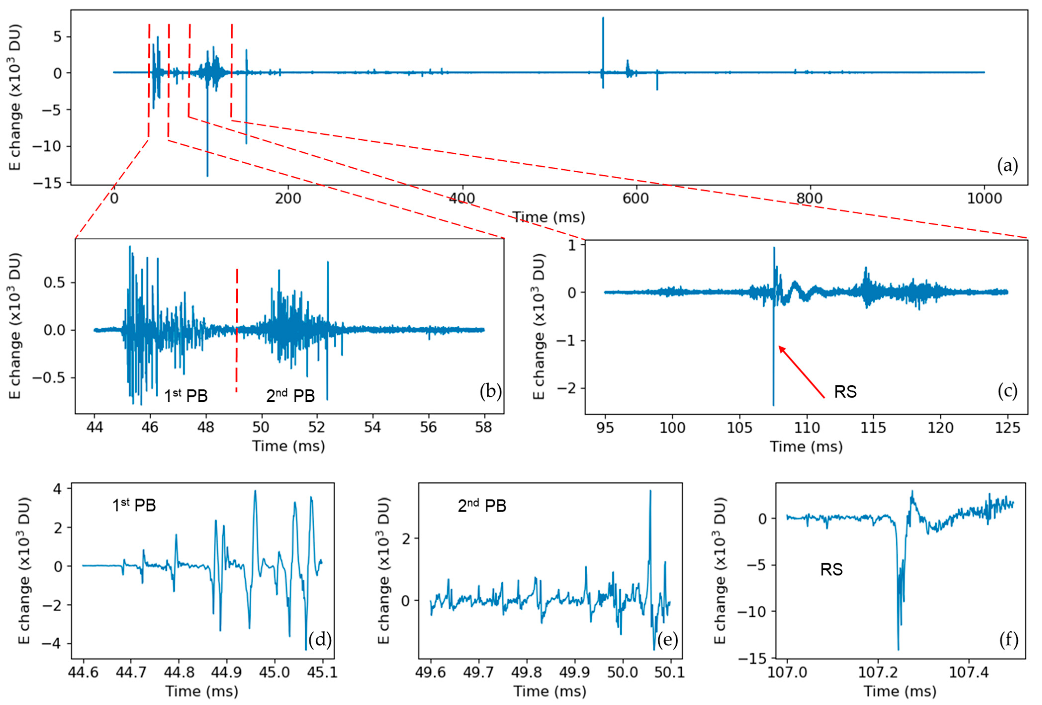
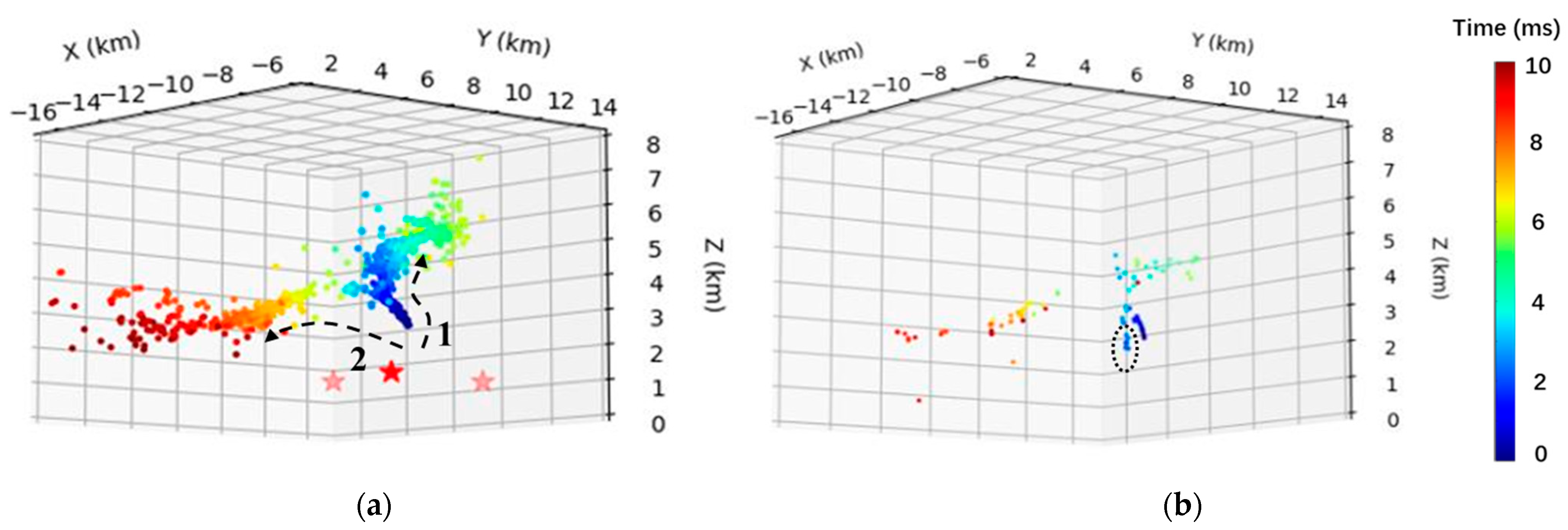
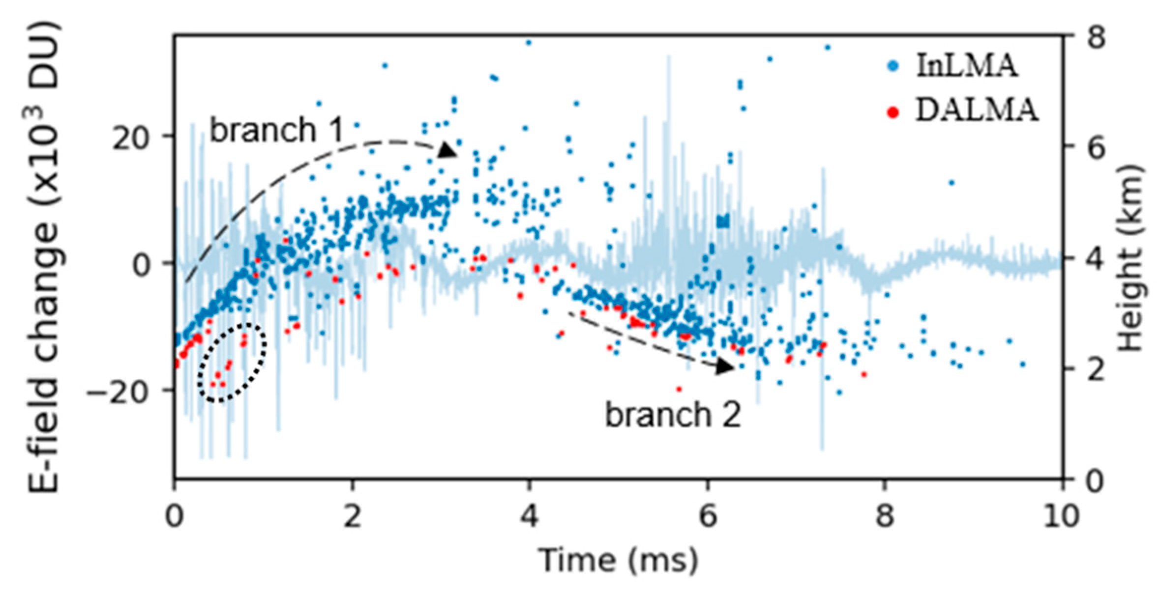
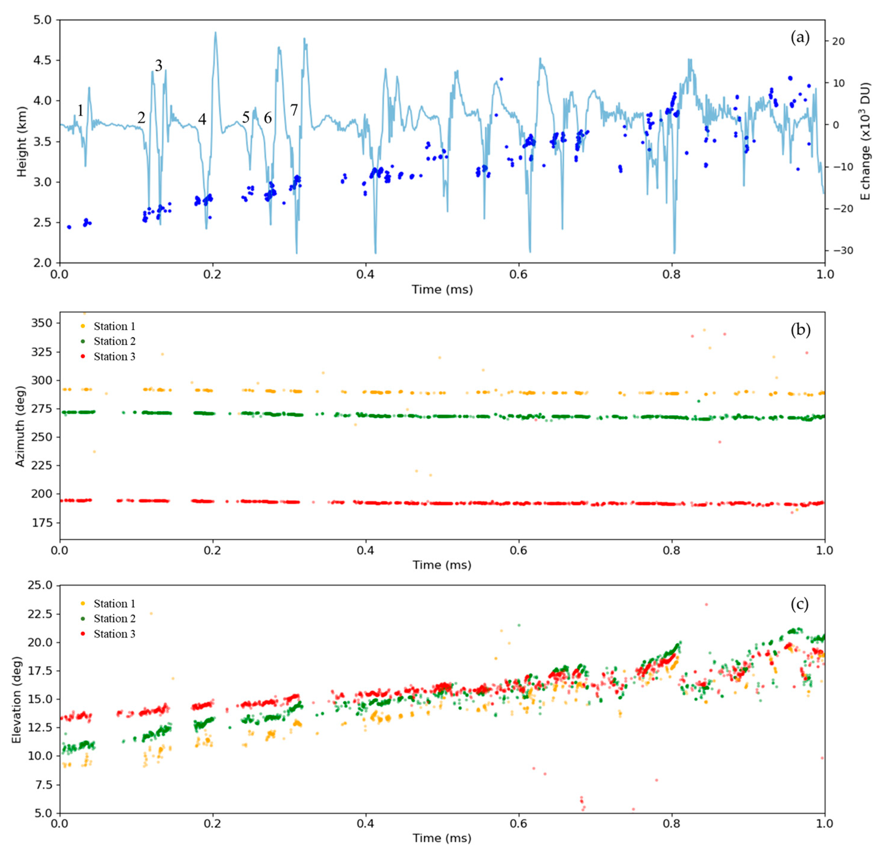
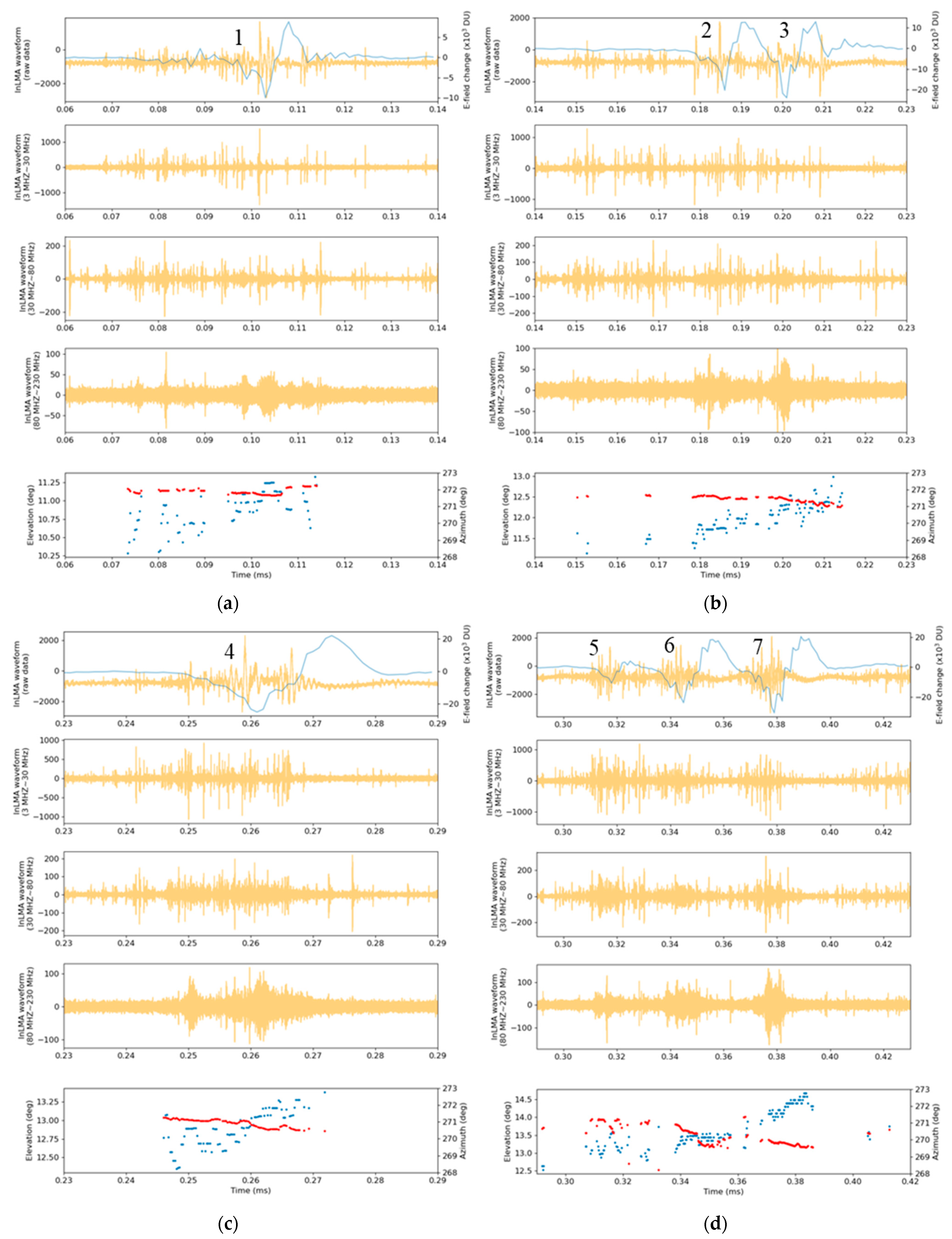
4.3. An Attempt to Better Characterize Preliminary Breakdowns

Preliminary breakdown processes have been studied by many authors [25,26,27,28]. However, concerning each individual PB pulse, little is known about how and what happens. In this section, by taking advantage of InLMA, we try to reveal more detailed features for individual PB pulse processes.

Figure 11 shows the mapped height along with the three stations’ azimuths and elevations of PB pulse discharges during the initial 1 ms with (a) for height, (b) for azimuths, and (c) for elevations. For comparison, the corresponding E-field change is also included in Figure 11a. As evident in Figure 11b, the located points by station 1 are apparently much fewer than those by station 2 and station 3 due to the larger background noise at station 1. Since 3D located points are basically limited by the station with the fewest points, the height points in Figure 11a are also much fewer than the azimuth and elevation points of station 2 and station 3. Additionally, as seen in Figure 11, for all the individual PB discharges, particularly those numbered from one to seven with simple structures, there is consistently no considerable change in the corresponding azimuths, but the elevations vary significantly. The height variation in Figure 11a can be approximately treated as a 3D distance change. It appears that each PB pulse process has a spatial scale of around 150 m along its progression direction. Furthermore, we note that the sub-discharges of two adjacent pulse discharges for the pulses numbered from one to seven in Figure 11a consistently appear progressively in connection to each other, though they are discontinuous in time. The progression speed measured from pulse one to pulse seven is about 1.4 × 10⁶ m/s.

For these seven pulses, we have tried a more detailed analysis by comparing the waveforms of the E-field change, the raw InLMA data, the 3 MHz~30 MHz, 30 MHz~80 MHz, and 80 MHz~230 MHz bandpass data, and the corresponding azimuth and elevation mapped by station 3, as shown in Figure 12. Figure 12a–d have the same format, except for different pulses, with the top panel for E-field change, the second to the fourth panels for the 3 MHz–30 MHz, 30 MHz–80 MHz, and 80 MHz–230 MHz data, and the fifth panel for the azimuth and elevation.

As seen in Figure 12, all PB E-field change bipolar pulses are accompanied by HF and VHF signals. For each individual bipolar pulse with a negative pulse appearing first and a positive pulse following, the corresponding HF and VHF signals tend to occur at the leading edge of the initial negative pulse. These HF and VHF signals tend to peak around the negative pulse peak and then disappear with the end of the negative pulse, which is generally consistent with the findings made by Kolmasova et al. [29] for VHF signals. During the positive part of the bipolar pulse, the HF and VHF signals are usually weak. We can also note some differences in the different bands of the signals. At a higher frequency band, such as 80 MHz–230 MHz, the VHF signals tend to vary continuously. In contrast, at a lower frequency band, such as 3 MHz–30 MHz, the HF signals tend to vary more or less in a discrete manner. Usually, the higher the frequency is, the smaller the scale of the source discharge. This finding appears to indicate that smaller scale (about 1–4 m, estimated from the corresponding electromagnetic wave length) discharges during the leading edge of the negative pulse occur almost continuously, while the larger scale (larger than 10 m) discharges occur in a discrete manner. During the earlier stage of the leading edge of each negative pulse, the located discharge sources tend to scatter in a wider range of elevation. At the timing of the negative pulse peak, the discharge sources tend to scatter in a narrow range of elevation. From the elevation variation patterns during the leading edge, we can also identify several progressions. Some of these progressions appear to move in upward directions (or forward directions), while others are in downward directions (or backward directions). The typical speed of these progressions is estimated to be around 6.0 × 10⁷ m/s. Interestingly, this speed is comparable to those for fast positive breakdowns [30,31] and also for fast negative breakdowns [32].

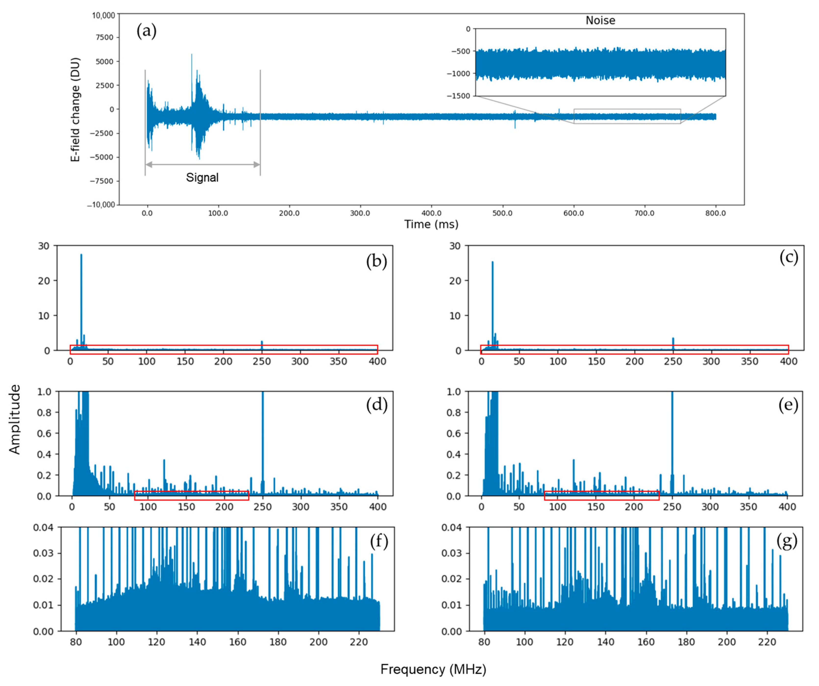
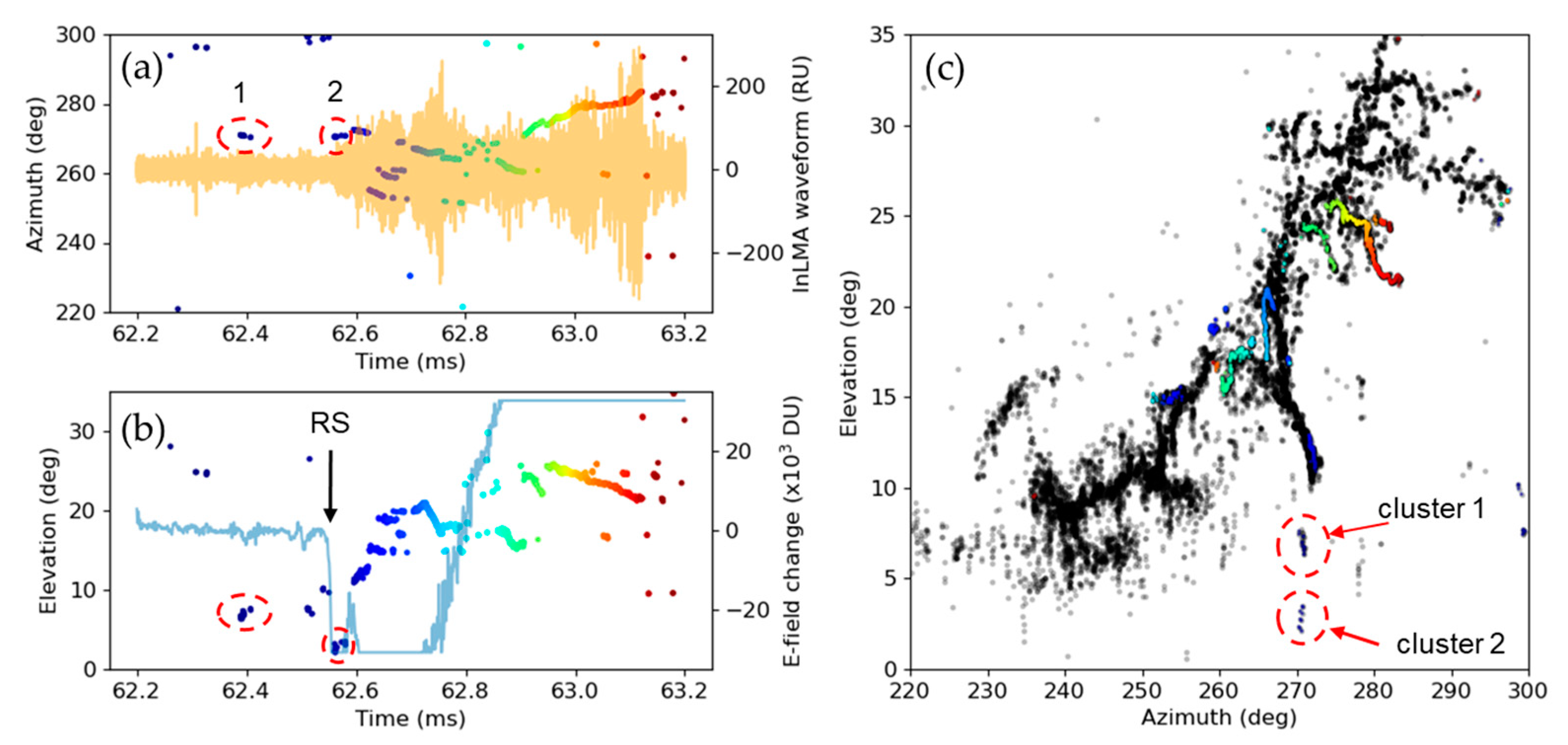
4.4. An Attempt to Characterize the Positive Return Stroke

Using a narrow band interferometer, Shao et al. have mapped several negative return strokes (RS) in two dimensions [33]. Using a broadband interferometer, Li et al. have succeeded in mapping two negative RSs in rocket-triggered lightning in three dimensions [34]. Perhaps due to the rarity of positive return strokes, their mapping results and thus the relevant characteristics have never been reported before. This motivates us to have a try to map the positive return stroke observed in this study. We chose the 2D mapping result by InLMA station 3 for this analysis since it mapped more points than the remaining two stations. Shown in Figure 13 are the azimuth and raw InLMA waveform (a), elevation and E-field change (b), and the 2D elevation versus azimuth view.

About 200 μs before the return stroke, there are several sources located at the elevation from 7° to 8° and the azimuth of 270°. These sources are denoted as cluster 1 in Figure 13. Then, at the initial stage of the return stroke, another cluster of sources, denoted as cluster 2, are located. Cluster 2 is at the elevation from 2°−3° and the azimuth of 270°. During the following 20 μs, there are no sources located near cluster 2. Many sources began to be located along the channel of the initial upward leader with a clear upward progression, followed by several clear progressions in bright colors along the previous discharge channels. Unfortunately, cluster 2 did not show a clear upward progression. However, if we assume that the return stroke wave propagated straightly from cluster 2 to the lightning initiation point, we can get a 3D progression speed of about 7.5 × 10⁷ m/s. This speed is smaller than those for most return strokes, which are usually measured near ground by optical means [35,36]. Since return strokes tend to have a decreasing speed when they go up [37], their average speeds along their entire channels should be smaller. Indeed, for one negative return stroke, Shao et al. reported an average speed of 3–5 × 10⁷ m/s [33]. We believe that the average speed that we measured is reasonable.

5. Discussion and Concluding Remarks

To the best of our knowledge, the lightning mapping system reported in this paper is the first lightning mapping array that is formed by three broadband interferometers. The method proposed in this paper for conducting 3D mapping with multiple interferometers is also new. Although the system demonstrated in this paper only consists of three stations, it can be readily expanded to have more stations. More stations can not only cover a wider area, but also reduce uncertainty in the mapping, similar to the lightning mapping array using TOA techniques. In order to observe winter lightning in Japan, whose discharge sources usually occur with lower heights, we intentionally limited the distances between stations. In the cases of observing summer lightning, whose discharge sources usually occur at higher heights, we think the station distances can be increased to more than 10 km. In such cases, the cross correlation between stations may become difficult. As a matter of fact, in the method we propose, even without the cross correlation between stations, 3D mapping can still be achieved only by using the azimuth and elevation information of each station.

Despite the lightning analyzed in this study being more than 10 km away from our InLMA stations, we can still perform some detailed mappings, particularly for the PB processes, which exhibited two stages. Interestingly, these two stages of PB processes occurred, respectively, along two branches with completely different orientations. The corresponding charge structure must be very complicated. Each individual PB pulse involves many small-scale discharges that usually scatter in a vertical scale of around 150 m. The smaller scale (1–4 m scale) discharges appear continuously in time but scatter in a wider range of height, while discharges with a scale of about 10 m tend to occur in a discrete manner. For some small-scale discharges, we can identify their progressions. The PB pulse itself should be a discharge with a scale of some hundred meters, which tends to be located at a lower height than its small-scale discharges. Our results on PB pulse discharges appear to support the PB model proposed by Shi et al. [28]. Furthermore, some of the small-scale discharges appear to propagate forward, while the others appear to propagate backward. Both the forward and backward progressions have a typical speed of 6.0 × 10⁷ m/s. Since this speed is comparable to the speeds of the fast positive breakdowns [30] and of the fast negative breakdowns [32], our results may indicate that a PB process may involve both fast positive breakdown (backward progression here) and fast negative breakdown (forward progression here), though in smaller scales compared with those of conventional fast breakdowns [30,32].

During the upward progression of a positive return stroke, its wavefront should be a kind of negative breakdown. Since a negative breakdown usually radiates more VHF signals than a positive breakdown in front of a negative return stroke, a positive return stroke should be mapped more easily by an interferometer. However, in this study, InLMA did not detect the positive return stroke itself during the period when the stroke was propagating along the channel of its positive leader. Perhaps this is due to the far distance between the return stroke and InLMA. After the return stroke enters into the PB channels, the relevant progressions have been mapped with much more defined channels than the PB processes.

The far distance of the lightning data prevents us from performing more detailed analyses on various lightning discharge processes. In the future, we will try to record some close distance lightning and try narrower windows and smaller sliding steps to improve the temporal and spatial resolutions. We believe that InLMA will allow us to uncover many complicated discharge features of winter lightning in Japan.

References

1. Wang, D.; Wu, T.; Takagi, N. Charge Structure of Winter Thunderstorm in Japan: A Review and an Update. IEEJ Trans. Power Energy 2018, 138, 310–314. [Google Scholar] [CrossRef]
2. Zheng, D.; Wang, D.; Zhang, Y.; Wu, T.; Takagi, N. Charge regions indicated by LMA lightning flashes in Hokuriku’s winter thunderstorms. J. Geophys. Res. Atmos. 2019, 124, 7179–7206. [Google Scholar] [CrossRef]
3. Huang, H.; Wang, D.; Yang, J.; Wu, T.; Takagi, N. Complicated aspects of a CG lightning flash observed in winter storm in Japan. J. Atmos. Electr. 2022, 41, 11–29. [Google Scholar] [CrossRef]
4. Wang, D.; Wu, T.; Huang, H.; Yang, J.; Yamamoto, K. 3D Mapping of Winter Lightning in Japan with an Array of Discone Antennas. IEEJ Trans. Electr. Electron. Eng. 2022, 7, 1606–1612. [Google Scholar] [CrossRef]
5. Stock, M.G.; Akita, M.; Krehbiel, P.R.; Rison, W.; Edens, H.E.; Kawasaki, Z.; Stanley, M.A. Continuous broadband digital interferometry of lightning using a generalized cross-correlation algorithm. J. Geophys. Res. Atmos. 2014, 119, 3134–3165. [Google Scholar] [CrossRef]
6. Warwick, J.W.; Hayenga, C.O.; Brosnahan, J.W. Interferometric directions of lightning sources at 34 MHz. J. Geophys. Res. Atmos. 1979, 84, 2457. [Google Scholar] [CrossRef]
7. Rhodes, C.T.; Shao, X.M.; Krehbiel, P.R.; Thomas, R.J.; Hayenga, C.O. Observations of lightning phenomena using radio interferometry. J. Geophys. Res. Atmos. 1994, 99, 13059–13082. [Google Scholar] [CrossRef] [Green Version]
8. Shao, X.M.; Holden, D.N.; Rhodes, C.T. Broad band radio interferometry for lightning observations. Geophys. Res. Lett. 1996, 23, 1917–1920. [Google Scholar] [CrossRef]
9. Ushio, T.-O.; Kawasaki, Z.-I.; Ohta, Y.; Matsuura, K. Broad band interferometric measurement of rocket triggered lightning in Japan. Geophys. Res. Lett. 1997, 24, 2769–2772. [Google Scholar] [CrossRef]
10. Akita, M.; Stock, M.; Kawasaki, Z.; Krehbiel, P.; Rison, W.; Stanley, M. Data processing procedure using distribution of slopes of phase differences for broadband VHF interferometer. J. Geophys. Res. Atmos. 2014, 119, 6085–6104. [Google Scholar] [CrossRef]
11. Yoshida, S.; Biagi, C.J.; Rakov, V.A.; Hill, J.D.; Stapleton, M.V.; Jordan, D.M.; Uman, M.A.; Morimoto, T.; Ushio, T.; Kawasaki, Z.-I. Three-dimensional imaging of upward positive leaders in triggered lightning using VHF broadband digital interferometers. Geophys. Res. Lett. 2010, 37, L05805. [Google Scholar] [CrossRef]
12. Liu, H.; Dong, W.; Wu, T.; Zheng, D.; Zhang, Y. Observation of compact intracloud discharges using VHF broadband interferom-eters. J. Geophys. Res. Atmos. 2012, 117, D01203. [Google Scholar]
13. Jensen, D.P.; Sonnenfeld, R.G.; Stanley, M.A.; Edens, H.E.; da Silva, C.L.; Krehbiel, P.R. Dart-leader and k-leader velocity from initiation site to termination time-resolved with 3d interferometry. J. Geophys. Res. Atmos. 2021, 126, e2020JD034309. [Google Scholar] [CrossRef]
14. Thyer, N. Double Theodolite Pibal Evaluation by Computer. J. Appl. Meteorol. 1962, 1, 66–68. [Google Scholar] [CrossRef]
15. Liu, H.; Qiu, S.; Dong, W. The Three-Dimensional Locating of VHF Broadband Lightning Interferometers. Atmosphere 2018, 9, 317. [Google Scholar] [CrossRef] [Green Version]
16. Mardiana, R.; Kawasaki, Z.-I.; Morimoto, T. Three-dimensional lightning observations of cloud-to-ground flashes using broadband interferometers. J. Atmos. Sol.-Terr. Phys. 2002, 64, 91–103. [Google Scholar] [CrossRef]
17. Wang, D.; Takagi, N. Characteristics of Winter Lightning that Occurred on a Windmill and its Lightning Protection Tower in Japan. IEEJ Trans. Power Energy 2012, 132, 568–572. [Google Scholar] [CrossRef]
18. Wu, T.; Wang, D.; Takagi, N. Lightning Mapping with an Array of Fast Antennas. Geophys. Res. Lett. 2018, 45, 3698–3705. [Google Scholar] [CrossRef]
19. Wu, T.; Wang, D.; Takagi, N. Upward Negative Leaders in Positive Upward Lightning in Winter: Propagation Velocities, Electric Field Change Waveforms, and Triggering Mechanism. J. Geophys. Res. Atmos. 2020, 125, e2020JD032851. [Google Scholar] [CrossRef]
20. Lyu, F.; Cummer, S.A.; Qin, Z.; Chen, M. Lightning Initiation Processes Imaged with Very High Frequency Broadband Interferometry. J. Geophys. Res. Atmos. 2019, 124, 2994–3004. [Google Scholar] [CrossRef]
21. Shao, X.M.; Ho, C.; Bowers, G.; Blaine, W.; Dingus, B. Lightning interferometry uncertainty, beam steering interferometry, and ev-idence of lightning being ignited by a cosmic ray shower. J. Geophys. Res. Atmos. 2020, 125, e2019JD032273. [Google Scholar] [CrossRef]
22. Yin, W.; Jin, W.; Zhou, C.; Liu, Y.; Tang, Q.; Liu, M.; Chen, G.; Zhao, Z. Lightning detection and imaging based on VHF radar inter-ferometry. Remote Sens. 2021, 13, 2065. [Google Scholar] [CrossRef]
23. Wu, T.; Wang, D.; Takagi, N. Multiple-stroke positive cloud-to-ground lightning observed by the FALMA in winter thunderstorms in Japan. J. Geophys. Res. Atmos. 2020, 125, e2020JD033039. [Google Scholar] [CrossRef]
24. Yang, J.; Wang, D.; Huang, H.; Wu, T.; Takagi, N.; Yamatomo, K. Development of an Interferometer-type Lightning Mapping Array System. In Proceedings of the 2022 36th International Conference on Lightning Protection (ICLP), Cape Town, South Africa, 2–7 October 2022; pp. 350–353. [Google Scholar]
25. Wu, T.; Takayanagi, Y.; Funaki, T.; Yoshida, S.; Ushio, T.; Kawasaki, Z.-I.; Morimoto, T.; Shimizu, M. Preliminary breakdown pulses of cloud-to-ground lightning in winter thunderstorms in Japan. J. Atmos. Sol.-Terr. Phys. 2013, 102, 91–98. [Google Scholar] [CrossRef]
26. Wu, T.; Yoshida, S.; Akiyama, Y.; Stock, M.; Ushio, T.; Kawasaki, Z. Preliminary breakdown of intracloud lightning: Initiation altitude, propagation speed, pulse train characteristics, and step length estimation. J. Geophys. Res. Atmos. 2015, 120, 9071–9086. [Google Scholar] [CrossRef] [Green Version]
27. Marshall, T.; Bandara, S.; Karunarathne, N.; Karunarathne, S.; Kolmasova, I.; Siedlecki, R.; Stolzenburg, M. A study of lightning flash initiation prior to the first initial breakdown pulse. Atmos. Res. 2018, 217, 10–23. [Google Scholar] [CrossRef]
28. Shi, D.; Wang, D.; Wu, T.; Takagi, N. Temporal and Spatial Characteristics of Preliminary Breakdown Pulses in Intracloud Lightning Flashes. J. Geophys. Res. Atmos. 2019, 124, 12901–12914. [Google Scholar] [CrossRef]
29. Kolmasova, I.; Marshall, T.; Bandara, S.; Karunarathne, S.; Stolzenburg, M.; Karunarathne, N.; Siedlecki, R. Initial Breakdown Pulses Accompanied by VHF Pulses During Negative Cloud-to-Ground Lightning Flashes. Geophys. Res. Lett. 2019, 46, 5592–5600. [Google Scholar] [CrossRef]
30. Rison, W.; Krehbiel, P.R.; Stock, M.G.; Edens, H.E.; Shao, X.-M.; Thomas, R.J.; Stanley, M.A.; Zhang, Y. Observations of narrow bipolar events reveal how lightning is initiated in thunderstorms. Nat. Commun. 2016, 7, 10721. [Google Scholar] [CrossRef] [Green Version]
31. Stock, M.G.; Krehbiel, P.R.; Lapierre, J.; Wu, T.; Stanley, M.A.; Edens, H.E. Fast positive breakdown in lightning. J. Geophys. Res. Atmos. 2017, 122, 8135–8152. [Google Scholar] [CrossRef]
32. Tilles, J.N.; Liu, N.; Stanley, M.A.; Krehbiel, P.R.; Rison, W.; Stock, M.G.; Dwyer, J.R.; Brown, R.; Wilson, J. Fast negative breakdown in thunderstorms. Nat. Commun. 2019, 10, 1648. [Google Scholar] [CrossRef] [PubMed] [Green Version]
33. Shao, X.M.; Krehbiel, P.R.; Thomas, R.J.; Rison, W. Radio interferometric observations of cloud-to-ground lightning phenomena in Florida. J. Geophys. Res. Atmos. 1995, 100, 2749–2783. [Google Scholar] [CrossRef]
34. Li, Y.; Qiu, S.; Shi, L.; Wang, T.; Zhang, Q.; Lei, Q.; Sun, Z. Observed Variation of Three-Dimensional Return Stroke Speeds Along the Channel in Rocket-Triggered Lightning. Geophys. Res. Lett. 2018, 45, 12569–12575. [Google Scholar] [CrossRef]
35. Idone, V.P.; Orville, R.E. Lightning return stroke velocities in the thunderstorm research international program (TRIP). J. Geophys. Res. Atmos. 1982, 87, 4903–4916. [Google Scholar] [CrossRef]
36. Jordan, D.M.; Rakov, V.A.; Beasley, W.H.; Uman, M.A. Luminosity characteristics of dart leaders and return strokes in natural lightning. J. Geophys. Res. Atmos. 1997, 102, 22025–22032. [Google Scholar] [CrossRef]
37. Wang, D.; Takagi, N.; Watanabe, T.; Rakov, V.A.; Uman, M.A. Observed leader and return-stroke propagation characteristics in the bottom 400 m of a rocket-triggered lightning channel. J. Geophys. Res. Atmos. 1999, 104, 14369–14376. [Google Scholar] [CrossRef]
Figure 1. Schematic of the interferometer hardware at one station.
Remotesensing 15 01923 g001
Figure 2. Antenna site map of InLMA, DALMA, and FALMA with the filling color representing the height above sea level.
Remotesensing 15 01923 g002
Figure 3. Illustration of three station InLMA with an assumed point discharge source ( x , y , z ) which radiates electromagnetic waves to the three stations. The corresponding angles are denoted and used to find the 3D location of the source ( x , y , z ) .
Remotesensing 15 01923 g003
Figure 4. (a) Flow chart used in 3D mapping program; (b) Description of the method for finding the time arrival differences windows between two stations.
Remotesensing 15 01923 g004
Figure 5. E-field change recorded at one station of FALMA. (a) 1 s of waveform; (b) waveform from 44 ms to 58 ms including two preliminary breakdowns; (c) waveform of the return stroke; (df) Expanded waveforms to indicate the 1st preliminary breakdown stages and the 2nd preliminary breakdown and return stroke in detail. The “atmospheric electricity” sign convention is used.
Remotesensing 15 01923 g005
Figure 6. 3D mapping result of the lightning flash by DALMA color-coded in time. Three pentagrams represent stations of InLMA. (a) 3D mapping; (b) Top view.
Remotesensing 15 01923 g006
Figure 7. Example waveform and frequency spectrum of the raw lightning data recorded at one channel of InLMA. (a) Signal waveform and background noise; (b,d,f) Frequency spectrum of the flash signal; (c,e,g) Frequency spectrum of the noise.
Remotesensing 15 01923 g007
Figure 8. 2D result from station 3 of InLMA. (a) Azimuth result with InLMA waveform versus time; (b) Elevation result with E-field change versus time; (c) 2D view of azimuth versus elevation with two branches, 1 and 2, identified.
Remotesensing 15 01923 g008
Figure 9. A comparison between 3D mapping results of InLMA and DALMA for the initial 10 ms of the flash. (a) 3D mapping of InLMA with locations of three stations of InLMA. (b) 3D location result from DALMA.
Remotesensing 15 01923 g009
Figure 10. A comparison between the 3D heights mapped by InLMA and DALMA along with the corresponding E-field change.
Remotesensing 15 01923 g010
Figure 11. Mapping results for the PB pulses occurred during the initial 1 ms stage. (a) 3D mapping by InLMA along with the E-field change. The pulses numbered from one to seven have a simple structure and will be studied further next; (b) Azimuth versus time for all three InLMA stations; (c) Elevation versus time for all three InLMA stations.
Remotesensing 15 01923 g011
Figure 12. The raw InLMA data (top panel in orange), the 3 MHz~30 MHz, 30 MHz~80 MHz, and 80 MHz~230 MHz bandpass data (the second, the third, and the fourth panels), and the corresponding azimuth and elevation (the fifth or the bottom panel in red and blue, respectively) along with the E-field change (top panel in blue) with (a) for pulse 1, (b) for pulses 2 and 3, (c) for pulse 4, and (d) for pulses 5, 6, and 7.
Remotesensing 15 01923 g012
Figure 13. 2D mapping result of the discharge processes around the positive return stroke. (a) Azimuth and InLMA raw waveform; (b) Elevation and FALMA E-field change (c) 2D vertical view of elevation versus azimuth. Black points are all discharge sources occurring during the period from lightning initiation until 62.2 ms later; color points coded in time are the discharge sources during the period around the positive return stroke. Two clusters are circled with red dotted lines, with cluster 1 occurring before the return stroke, likely due to the downward positive leader of the stroke, while cluster 2 occurs at the initial stage of the return stroke.
Remotesensing 15 01923 g013
Disclaimer/Publisher’s Note: The statements, opinions and data contained in all publications are solely those of the individual author(s) and contributor(s) and not of MDPI and/or the editor(s). MDPI and/or the editor(s) disclaim responsibility for any injury to people or property resulting from any ideas, methods, instructions or products referred to in the content.