Abstract
Food and economic security in West Africa rely heavily on rainfed agriculture and are threatened by climate change and demographic growth. Accurate rainfall information is therefore crucial to tackling these challenges. Particularly, information about the occurrence and length of droughts as well as the onset date of the rainy season is essential for agricultural planning. However, existing rainfall models fail to accurately represent the highly variable and sparsely monitored West African rainfall patterns. In this paper, we show the potential of deep learning (DL) to model rainfall in the region and propose a methodology to develop DL models in data-scarce areas. We built two DL models for satellite rainfall (rain/no-rain) detection over northern Ghana from Meteosat TIR data based on standard DL architectures: Convolutional neural networks (CNNs) and convolutional long short-term memory neural networks (ConvLSTM). The Integrated Multi-satellitE Retrievals for the Global Precipitation Measurement (GPM) mission (IMERG) and Precipitation Estimation from Remotely Sensed Imagery Using an Artificial Neural Network Cloud Classification System (PERSIANN-CCS) products are used as benchmarks. We use rain gauge data from the Trans-African Hydro-Meteorological Observatory (TAHMO) for model development and performance evaluation. We show that our models compare well against existing products despite being considerably simpler, developed with a small training dataset—i.e., 8 stations covering 2.5 years with 20.4% of the data missing—and using TIR data alone. Concretely, our models consistently outperform PERSIANN-CCS for rain/no-rain detection at a sub-daily timescale. While IMERG is the overall best performer, the DL models perform better in the second half of the rainy season despite their simplicity (i.e., up to 120 k parameters). Our results suggest that DL-based regional models are a promising alternative to state-of-the-art global products for providing regional rainfall information, especially in meteorologically complex regions such as the (sub)tropics, which are poorly covered by ground-based rainfall observations.
1. Introduction
Food and economic safety in West Africa depend heavily on rainfed agriculture and, therefore, on rainfall. In this context, accurate rainfall information is essential to ensure food security. Uncertainty in West African rainfall and the associated vulnerability of small-holder farmers have been documented since the last century. In the 1970s, the Sahelian Drought was socially and agriculturally devastating. It was reported to have produced 100,000 deaths by 1973 and was followed by continuous droughts in the next two decades [1,2]. Currently, climate change and global population growth [3], the two great threats of this century, exacerbate these problems. Sub-Saharan Africa will account for most of this century’s population growth and will become the world’s most populous area by the late 2060s [4]. Climate change is changing the onset of the rainy season over the Sahel [5] and causing more frequent droughts in most of Africa, which is severely increasing food insecurity [6,7]. Rainfall detection is essential to monitor these changes, characterize rainfall patterns, and supply the information needed for efficient agricultural planning. However, a sparse, unevenly distributed, and inconsistently reported rain gauge network poses a major challenge to studying rainfall variability in this region—and has been a persistent problem since the last century [8].
Satellite rainfall products are of special relevance for areas with sparse rain gauge networks, such as sub-Saharan Africa, because of their global coverage. In fact, satellite rainfall retrieval and its application over Africa have been in constant development since the late 1960s [8,9,10,11]. However, existing satellite products show a poor correlation with ground measurements in the region. For example, the Africa Climate Hazards Infrared Precipitation with Stations (CHIRPS) [12] and the Tropical Applications of Meteorology Using Satellite Data and Ground-Based Observations (TAMSAT) [13], particularly developed for Africa based on the Cold Cloud Duration method, show daily Kling–Gupta Efficiency values below 0.4 [14,15]. The most widely used machine learning-based product, Precipitation Estimation from Remotely Sensed Information using Artificial Neural Networks-Cloud Classification System (PERSIANN-CCS) [16], tends to have a high false alarm ratio (FAR) and to overestimate rainfall both globally and in Africa [17,18]. Lastly, the Global Precipitation Measurement (GPM) Integrated Multi-satellitE Retrievals for GPM (IMERG) [19], which combines both physical and ML-based methods and has been developed to become the longest and most detailed rainfall data set, show a weaker correlation with ground measurements in West Africa than in other regions of the world [20,21].
The literature suggests that an important reason for the poor performance of satellite rainfall estimates over West Africa is the sparse rain gauge distribution, leading to underrepresentation in the training or calibration data for the modeling algorithms. Additionally, atmospheric conditions differ from other regions in the world, as there are higher aerosol concentrations, higher land surface temperatures, and a generally drier atmosphere [22]. Furthermore, the generalization performance of existing ML rainfall retrieval models trained on dense gridded rainfall data [16,23,24,25] may decrease for areas with less training data and different atmospheric conditions.
Deep learning (DL) is becoming increasingly popular in the field of environmental remote sensing because of its ability to learn complex patterns and features from data [26]. DL methods exploit spatial and sequential inductive biases to improve performance by incorporating the assumption that nearby pixels in an image and nearby elements in a sequence have more relevance to the output, which allows the network to learn more effectively and generalize to new examples.
In this work, we investigate whether locally training a deep learning model can overcome the limitations of global products in capturing the complex rainfall dynamics of this region. We develop two models based on CNN and ConvLSTM for rain/no-rain detection in the data-scarce region of northern Ghana, West Africa. Both models have been trained on a small regional dataset, representative of data availability in the region. The focus of this paper is on rain/no-rain detection, i.e., binary classification, as a first step towards rainfall intensity estimation. In Section 2, we present the data and study area and introduce our methodology; in Section 3, we report our results; in Section 4, we compare our findings with those of other studies; and in Section 5 we draw the main conclusions of this study and propose future work beyond this paper.
2. Materials and Methods
2.1. Model Development Datasets
The input to the model is level 1.5 data from the Spinning Enhanced Visible and InfraRed Imager (SEVIRI) instrument aboard the Meteosat Second Generation (MSG) satellite. Concretely, we use data from the 10.8 µm channel (channel 9 of SEVIRI), a window channel in the thermal infrared (TIR) region that is widely employed for rainfall estimation from cloud top temperature [27]. The spatial resolution over our study area is 3.1 km × 3.1 km [28]. The temporal resolution is 15 min.
2.2. Target Data: TAHMO Rain Gauge Data
To develop the models, we used hourly rain gauge data from the Trans-African Hydro-Meteorological Observatory (TAHMO) [29] as target data. TAHMO provides quality-controlled rainfall data, available in near real time. There are eight TAHMO stations in our study area during the research period (July 2018—December 2020). Their locations and characteristics are displayed in Figure 1 and Table 1, respectively. Table 1 also includes the number of rain events per station per year. Here, a rain event is defined as an uninterrupted time period of over-zero rainfall measurements with a cumulative rainfall of at least 1 mm, and there is a 1 h separation window between rain events.
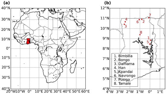
Figure 1.
(a) Ghana located in West Africa and (b) TAHMO stations considered in this study. UTM coordinates.

Table 1.
Description of the considered TAHMO stations, data gap percentage at hourly timescale and number of rain events during the study period (1 July 2018–31 December 2020).
2.3. Benchmark Products
We used two benchmark products for performance evaluation (Table 2): PERSIANN-CCS [16], as a reference operational ML-based satellite rainfall product, and IMERG [19], as a very high-quality global satellite rainfall product.
Table 2.
Summary of the characteristics of the benchmark products used in this study.
PERSIANN–CCS builds on its predecessor, PERSIANN [30], and estimates rainfall from GEO IR images. First, the model segments and classifies clouds into cloud patches based on manually selected features such as cloud texture or geometry. Second, it learns the relationship between brightness, temperature, and rainfall rates for each cloud patch [16]. PERSIANN-CCS has a latency of approximately 3 h. A possible limitation of this method lies in the human-assigned features and group definitions of cloud patches, which may be reductionist or faulty in representing physical (rainfall) processes that are not yet fully understood.
IMERG has been developed by NASA and is available as three different products with varying latency times and more data being incorporated in successive runs of the algorithm: Early run, with a 4 h latency time; Late run, with a 12 h latency time; and Final run, with a latency time of 3.5 months. NASA advises using the Final Run as research-ready data. Here, we evaluated all three products. The latest algorithm upgrade of IMERG at the time of writing this paper was version 06.
IMERG relies on multiple data sources and algorithms: It employs GEO IR satellites, “as many as possible” opportunistic LEO satellites, and monthly gauge analyses [19]. The LEO satellites provide PMW rainfall estimates that are propagated forwards and backwards in time using estimated rainfall motion vectors. GEO IR estimates are added using the PERSIANN-CCS algorithm to fill in the gaps between LEO PMW estimates. The Early Run of the algorithm only has forward propagation, whereas the Late Run has both forward and backward propagation, allowing for interpolation. Furthermore, the longer latency time allows for lagging data transmissions that might have been missed in the Early Run to be incorporated in the Late Run. The gauge analyses from the Global Precipitation Climatology Centre (GPCC) are used to regionalize and correct biases in the final stage of the algorithm. Other input data are the GPM Combined Radar-Radiometer (CORRA) rainfall estimates, Modern-Era Retrospective Analysis for Research and Applications Version 2 (MERRA-2), and Goddard Earth Observing System model (GEOS) Forward Processing (FP) precipitable water vapor data [19].
2.4. Study Area: North of Ghana
Northern Ghana, defined here as the northern part of Ghana comprising the five northern regions and not the northern region alone, lies between latitudes 8°N and 11°N and longitudes 3°W and 0°30′E and is situated in the Savanna climatic zone. It is heavily affected by high variability in climate and hydrological fluxes, with frequent floods and droughts accompanied by high temperatures. This produces frequent crop failures or losses, outbreaks of diseases, and dislocation of human populations, with major economic repercussions [31]. Over 70% of employment in Ghana is in near-subsistence agriculture in rural areas [32].
Ghana’s climate is characterized by markedly seasonal rainfall with high interannual variability. Rainfall seasons are determined by the movement of the intertropical convergence zone (ITCZ), which oscillates between the north and south tropics throughout the year [32]. The ITCZ separates a cold, moist air mass moving northward from the Atlantic and a dry, hot, and dusty air mass from the Sahara Desert. As opposed to the south of Ghana, which has two annual rainy seasons, northern Ghana has a unimodal rainfall regime, with a rainy season from March to October, when the ITCZ is in its northernmost position [32,33]. Figure 2 shows the average monthly temperature and rainfall in Bawku, in the upper-east region of Ghana, which is representative of the climatology of the region. Over 75% of rainfall in this area is due to deep convection, most of it organized as large mesoscale convective systems [34]. Intense and short-lived events as a result of deep convection characterize the diurnal rainfall variation in this region [35]. For example, over 80% of rain events present in our development dataset last less than 3 h.
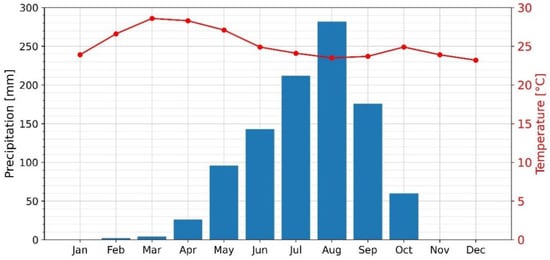
Figure 2.
Average monthly temperature and rainfall in Bawku, upper-east region, Ghana (1993–2011). Data adapted from [36]. Bawku is representative of the climatology of our study area: the five northern regions of Ghana.
2.5. Data Preprocessing
Figure 3 shows the flow diagram of the overall methodology presented in this research, with special detail given to the data preprocessing stage.
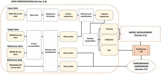
Figure 3.
Overall flow diagram of the methodology followed in this study, from data preprocessing to performance comparison.
One-hour TAHMO and thirty minute IMERG data were accumulated in 3 h intervals, while PERSIANN-CCS data were directly obtained with a 3 h resolution. All three products were classified as rain/no-rain using a 1 mm/3 h threshold.
Data scarcity poses an obstacle to DL-based rainfall estimation or prediction, in that the existence of densely gridded data to use as training data during model development is a pre-requisite for most existing approaches [16,23,24,25]. Our study area has a sparse rain gauge distribution, with distances between stations too large to allow reliable interpolation, especially considering the highly localized rainfall patterns in West Africa. We employ a methodology to overcome this obstacle by using point-based instead of gridded data as the output of the model. RainRunner utilizes an image-to-point approach: the model is trained only with point-based rainfall data, corresponding to the center of the input image. Some studies [37,38] have used a similar methodology, cropping satellite data around rain gauge measurements used as target data before being input to a CNN in a DL model to estimate rainfall. However, both approaches use other rainfall measurements present in the cropped scene—and other data sources—as input to the models. [37] uses all rain gauges present in the scene, and [38] uses TRMM 34B2 precipitation data. In our case, MSG TIR images are the only model input, and they were cropped to create 32 pixels × 32 pixels (i.e., approx. 96 km × 96 km area) images centered on each TAHMO station as shown in Figure 4. Images were cropped in a way to ensure that the corresponding station fell in a “center square”, defined as a square with sides of length equal to the pixel size and with center on the geometrical center of the image. In this way, the model’s spatial resolution is the pixel size, i.e., approx. 3 km.
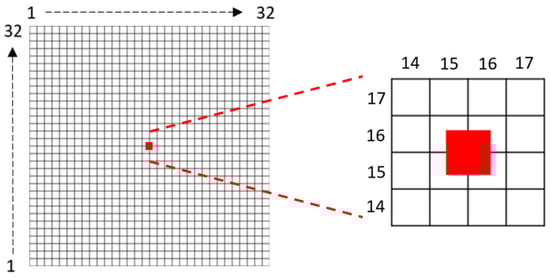
Figure 4.
Center square in a 32 × 32 pixels image. Here, pixels are numbered from bottom to top and from left to right.
Cropped MSG TIR images were grouped in 3 h sequences (i.e., groups of 12 images). Sequences were then classified as rain/no-rain according to the corresponding TAHMO data. Incomplete sequences due to gaps in TAHMO or MSG data were discarded. We chose a 3 h temporal resolution according to the short-lived rainfall events characteristic of this area. We expect this resolution to be able to capture the daily rainfall dynamics and deem a finer temporal resolution not needed for the end goal of our research, which is to improve the quality of rainfall information for agricultural applications.
To prepare the model development datasets, first we resampled the training dataset to deal with the data imbalance characteristic of rainfall binary classification [39]. We employed a 4:1 dry/rain ratio. Validation and test datasets were created with the same dry/rain ratio as the full 2020 data, i.e., 28.2:1, in order to be representative of reality. The data distribution is presented in Table 3.
Table 3.
Dataset distribution in training, validation, and test.
We assigned all 2018 and 2019 data to the training dataset. Out of the 2020 data, we randomly selected two sets of 250 rain sequences for the validation and test datasets; the rest were assigned to the training dataset.
After model development, its performance on the test dataset was evaluated through comparison to IMERG and PERSIANN-CCS. However, IMERG Final run and PERSIANN-CCS presented data gaps in the validation and test datasets. IMERG Final run had 241 gaps in the validation dataset and 229 in the test dataset, while PERSIANN-CCS only had 110 gaps in the validation dataset. Conveniently, so as not to penalize further the minority class, all corresponded to sequences recorded as dry by TAHMO stations. For a fair comparison, these sequences were removed during result evaluation.
2.6. Deep Learning Model
We framed the rainfall binary classification as a supervised binary classification problem. We developed two model architectures: RainRunner, based only on convolutional neural networks (CNN), and RainRunner-R, which incorporates a convolutional long short-term memory (ConvLSTM) architecture. Both models have the same input (sequences of 12 TIR images taken every 15 min) and output (rain/no-rain classification).
CNNs are deep neural networks with convolutional layers that exploit symmetries in gridded data by recognizing similar patterns and features, achieving efficient processing and generalization by reducing the number of learned parameters [40]. CNNs treat pixels as connected to their neighborhood instead of independent from each other through convolution and pooling operations [41]. This enables them to account for spatial correlations in rainfall. They are more computationally efficient than multi-layer perceptrons (MLPs) [18]. LSTM architectures are improved recurrent neural networks that incorporate a sequential inductive bias by means of memory cells and gates that selectively maintain and propagate important information across timesteps. This allows them to effectively process sequential data such as time series and natural language texts [42]. ConvLSTM [43] is an extension of LSTM to 2D sequences, i.e., images changing in time, instead of point-based time series. As such, they are suitable techniques to capture the spatio-temporal evolution of satellite gridded data.
We selected these relatively simple methods because of the nature of our problem. State-of-the-art (SOTA) methods for image classification and sequential processing based on transformers require tens of millions to a billion parameters to achieve top performances on benchmark datasets [44]. Training is performed using millions to billions (e.g., pre-training) of images and exceptional computing power [45]. These settings are very different from the case study we are considering, where we are dealing with fewer than ten thousand images. As such, it is beyond the scope of our paper to test very large SOTA models. Instead, we focus on more basic DL models capable of dealing with limited data to explore the overall suitability of the DL approach for this context. We employed ConvLSTM to test whether using a more suitable inductive bias to process our sequences would yield better results.
We differentiate two building blocks: CNN and ConvLSTM blocks. A CNN block comprises multiple convolution and pooling layers. The output of a CNN block is a feature map with dimensions greater than or equal to 8 × 8. The ConvLSTM block consists of ConvLSTM and batch normalization layers, with the output of the block being a 2D tensor. Besides these building blocks, we also used MLPs with a dropout layer between the hidden and output layers.
2.6.1. RainRunner Architecture
Upon receiving an image sequence, RainRunner processes each image in parallel through a CNN block and an MLP to produce one bounded real value (0,1) from each one of them. Then, these outputs are concatenated into a fully connected layer and passed through a second MLP to classify the 3 h input sequence as rain/no-rain. Figure 5 shows a schematic block diagram of this architecture.
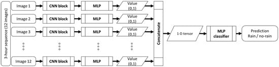
Figure 5.
Schematic block diagram of the RainRunner model architecture.
2.6.2. RainRunner-R Architecture
RainRunner-R processes all the images as a sequence through a ConvLSTM block. The output of this block is a 2D tensor that is then passed through a CNN block and an MLP to produce a rain/no-rain prediction. This architecture is shown in Figure 6. We investigated the effect of bidirectionality on the ConvLSTM architecture. Bidirectional recurrent neural networks allow training a model using both time directions (i.e., past to future, future to past) of the input when a whole sequence is available. While they cannot be used for forecasting purposes, they are particularly suitable for sequence recognition tasks such as ours [46].
Figure 6.
Schematic block diagram of the RainRunner-R model architecture.
2.7. Training and Hyperparameter Search
To account for data imbalance, we trained the models to minimize a weighted binary cross-entropy loss, where a weight of 0.8 was given to the rain class and 0.2 to the dry class (Equation (1)).
where N is the size of the dataset, y is the label/true value (i.e., 0 for no-rain and 1 for rain), and p(y) is the prediction probability (i.e., the estimated probability of each sequence i containing rain).
We trained multiple hyperparameter combinations and chose the best models based on a trade-off between the validation F1-score and the number of trainable parameters. We ran these models ten times and selected the overall best model for both RainRunner and RainRunner-R based on the validation F1-score. Using F1-score as a performance metric helps deal with the rain/dry data imbalance.
2.8. Performance Metrics and Misclassification Analysis
We used performance metrics commonly used in the meteorology field as well as the F1-score, a metric commonly used for imbalanced problems in DL, all extracted from the contingency table (Figure 7). Accuracy (Equation (2)) represents the number of correctly classified data samples out of all data samples; probability of detection (POD, Equation (3)) measures the ability of the model to correctly detect rain sequences; success rate and false alarm ratio (SR and FAR, Equation (4)) are complementary and represent the certainty with which rain sequences are detected; frequency bias (FBias, Equation (5)) represents the degree of correspondence between rain predictions and observation; finally, F1-score and critical success index (F1-score and CSI, Equations (6) and (7)) evaluate at the same time SR and POD.
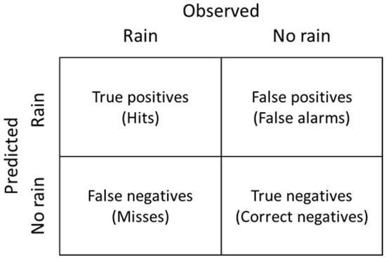
Figure 7.
Contingency table for the rain/no-rain binary classification problem.
POD, SR, F1score, and CSI can vary from 0 to 1, with 1 being the optimal value. FBias can range from 0 to ∞, with the optimal value being 1. If FBias is below 1, the events are under-forecasted; if it is greater than 1, they are over-forecasted.
We present results in three ways: as contingency tables, numerically as the forecast verification metrics, and visually in a Roebber diagram [47] or performance diagram.
To assess the generalization ability of the models in the context of the highly localized and seasonal rainfall in northern Ghana, we analyzed their performance depending on factors such as location and time of the year (Table 4) in terms of the distribution of misclassified sequences.
Table 4.
Factors considered for misclassification analysis. The “rain category” factor follows the definition of rain in the Glossary of Meteorology of the American Meteorological Society, AMS, except the “very light rain” category introduced here.
We compared the performance of RainRunner to that of the benchmark products by computing the forecast verification metrics and performing a misclassification analysis of all products. To assess the difference in performance of the three IMERG products–i.e., Early, Late, and Final Run—we included all of them in the forecast verification metrics computation. For the misclassification analysis, we used IMERG Final Run, as the highest-performing satellite rainfall product. We conducted the performance evaluation based on the results of the test dataset. For reference, we also include the forecast verification metrics of all products on the validation dataset.
3. Results
3.1. Selection of Best-Performing Model Architecture
We tested 48 hyperparameter combinations for both RainRunner and RainRunner-R and evaluated learning rates of 0.001, 0.0005, and 0.0001. We used a batch size of 32 and 400 epochs, with an early stopping criterion based on the improvement of the validation loss. We used an Adam optimizer [48].
The F1-score values of the tested model architectures ranged from close to 0 to almost 0.5 (Figure 8a), with the best-performing models doing so at the expense of a high number of trainable parameters (Figure 8b). Given the limited amount of data available for validation, we selected the simplest, best-performing architectures to reduce the chance of overly optimistic estimates of the model’s performance on unseen data [49]. We ran the chosen architectures ten times to select the overall best-performing models (Figure 8c). RainRunner achieved an overall higher validation F1-score but a lower median value than RainRunner-R. The model architectures that resulted in the best performances are shown in Figure 9. They consist of 120,125 parameters for RainRunner and 21,033 parameters for RainRunner-R, i.e., RainRunner-R has 17.5% of the trainable parameters of RainRunner. The best-performing architectures for both models had two concatenated convolution blocks (i.e., two convolutions + pooling operations). For the RainRunner-R model, a bidirectional ConvLSTM resulted in the best performances, which is in line with the classification task at hand, for which both time directions might contain useful information.
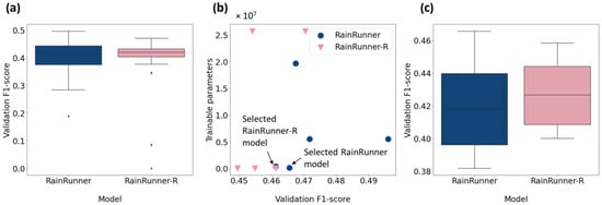
Figure 8.
Results of the hyperparameter search: (a) performance distribution of all tested model architectures; (b) number of trainable parameters and validation F1-score of the five model architectures with the highest validation F1-score; and (c) performance distribution of the selected models over 10 runs.
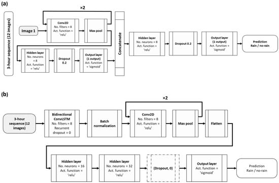
Figure 9.
Architecture of the best (a) RainRunner model (based on a CNN only) and (b) RainRunner-R model (combining ConvLSTM and CNN). In Figure 9a, only the pipeline of one image is shown, the other 11 images go through a similar CNN block.
3.2. Model Performance Evaluation
Table 5 shows the values of the performance metrics of the selected RainRunner models on our validation dataset, compared to those of PERSIANN-CCS and IMERG Early, Late, and Final run on the same dataset. RainRunner scored higher than PERSIANN-CCS on all metrics except FBias and achieves a POD similar to that of IMERG. The weakest point of RainRunner seems to be the substantially higher FBias.
Table 5.
Performance metrics on the validation dataset.
Figure 10 shows the contingency tables of the same models for our independent test dataset. IMERG Final run achieved the overall highest performance among all models, with 95% dry and 82% rain sequences correctly classified. IMERG Late and Early runs followed closely, with 95% (78%) and 95% (76%) dry (rain) sequences correctly classified, respectively. The remaining models achieved a similar performance in dry sequence classification: 94% for RainRunner, RainRunner-R, and PERSIANN-CCS. Lastly, both RainRunner models outperformed PERSIANN-CCS in rain sequence classification, with 74% of rain sequences correctly classified by RainRunner and 73% by RainRunner-R, as compared to 68% by PERSIANN-CCS. Finally, Figure 11 summarizes the performance scores in a Roebber diagram. A perfect model—with POD, CSI, and FBias equal to 1—would be in the upper-right corner of the diagram. We can see three clusters: the best performance corresponded to the three IMERG products, followed by the RainRunner models, and lastly, PERSIANN-CCS. RainRunner had the largest FBias, which indicates that it over-detected rain more often than the other models. In all the other performance metrics, the two RainRunner models outperformed PERSIANN-CCS on the test dataset.
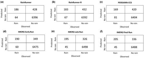
Figure 10.
Contingency tables of (a) RainRunner, (b) RainRunner-R, (c) PERSIANN-CCS, and (d) IMERG Early, (e) Late, and (f) Final run on the independent test dataset, consisting of 250 rain and 6824 dry sequences.
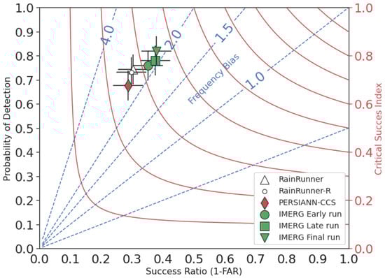
Figure 11.
Roebber performance diagram on the test dataset.
3.3. Misclassification Analysis
Figure 12 shows the distribution of misclassified sequences of the test dataset across individual stations, month of the year, and rain categories. About 4% to 10% of the sequences were misclassified across all stations. The southern stations showed a somewhat higher proportion of misclassified sequences than the northern stations. Seasonally, the percentage of misclassifications was much higher in the rainy season than in the dry season, when all models correctly classified nearly all sequences. IMERG performed better in the first half of the rainy season yet misclassified substantially more sequences in the second half of the rainy season, with up to 14% misclassifications for the month of September. For all models, the most challenging events to classify were very light and light rainfall, often misclassified as dry sequences. We also investigated the performance of the models in terms of misclassifications distributed over different times of the day (day/night), but there was no significant difference in the number of misclassifications for day and night.
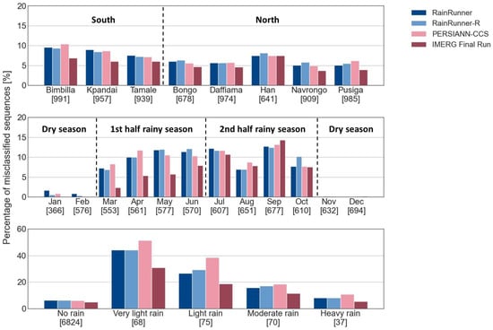
Figure 12.
Misclassification analysis according to (top) station, (center) month, and (bottom) rainfall intensity. The numbers in brackets below the x-axis represent the number of sequences of each category in the test dataset.
4. Discussion
Our findings show that DL models for rainfall binary classification trained with a small local dataset of strictly TIR data compare well to state-of-the-art global products. These results suggest three insights: (1) TIR data are strongly related to rainfall in this region; (2) DL can extract relevant features linking TIR images with rainfall; and (3) locally developing a DL model enables it to capture the characteristics of local processes, in this case, rainfall occurrence, better than some globally trained models.
The strong relationship between brightness temperature (Tb) and rainfall has been extensively studied and used for satellite rainfall retrieval. This relationship is particularly relevant in the Sahel, where around 75% of surface rainfall is due to deep convection that involves cold cloud tops, observable in TIR data [34]. RainRunner surpasses PERSIANN-CCS, which uses machine learning to link TIR data to rainfall through manually extracted features related to cloud properties. This shows that DL methods are able to extract relevant features from data and model natural processes better than expert-based models that rely on manual feature extraction. Especially training the model locally allows it to reproduce regional rainfall patterns more efficiently.
As seen in the Roebber performance diagram (Figure 10), all models over-predict rainfall with an FBias greater than 2. It is known that TIR-based methods over-predict rainfall because the size of large convection systems is much larger than the surface rainfall area underneath [34]. A further explanation of this over-prediction lies in the characteristic West African rainfall processes. Particularly, the presence of rain-bearing clouds does not necessarily mean rainfall on the ground. Sometimes rainfall does not reach the ground due to the higher concentration of aerosols and associated smaller drops, higher land surface temperature, and drier atmosphere compared to other regions [22]. Therefore, adding other relevant sources of information such as aerosols, land surface temperature, or water vapor data might improve the performance of the models. Furthermore, virga—precipitation evaporating before it reaches the ground—accounts for 15% of all precipitation profiles in the northern African Savanna (8°–12°N) [35]. Virga has been found to account for 50% of false PMW precipitation results in arid regions [50] and could be a cause for IMERG’s rainfall over-prediction. Furthermore, the presence of other MW radiation scatterers, such as dry sand, also results in satellite PMW retrievals over-estimating rainfall [35].
Despite the proven efficiency of DL methods to reproduce physical processes, data scarcity poses a challenge to their employment. To overcome this, we have used an image-to-point methodology that only needs point-based rainfall measurements. Although other studies have applied similar methodologies [37,38], they required additional rainfall information—additional rain gauges in the study region or a gridded satellite product—as model inputs. Compared to these, our approach has the advantage that it does not require any further rainfall information.
Of the two DL architectures we evaluated, results suggest that the temporal inductive bias introduced by the ConvLSTM architecture—processing each image in the 12-image sequence one after the other—does not improve model performance, although it results in a model with fewer trainable parameters (21,033 against 120,125 for RainRunner). The hyperparameter search in model design produced a wide range of performances for both models, which is probably explained by the relatively small training dataset. To investigate the robustness of the models, further research on a range of small to larger datasets would be needed. It is striking that our DL models based on TIR data only, developed with a small dataset and simple model architectures, achieve a performance close to that of IMERG. The high learning efficiency of the DL model, when trained with local data, is promising for the independent application of such models in data-scarce areas such as Sub-Saharan Africa. Additionally, it might be interesting to investigate combining the DL model with existing products such as IMERG, where the DL approach can offer complementary insights that help improve performance. For example, substituting the PERSIANN-CCS rainfall estimation scheme from TIR data within IMERG with our better-performing approach might improve IMERG’s estimations.
With most agriculture in West Africa being rainfed, access to accurate rainfall information is necessary for agricultural productivity. Satellite rainfall products, such as the one developed in this study, that, after training, can be interpolated to areas with no ground observations can play an essential role in overcoming the data scarcity challenge and contributing towards food and economic security.
5. Conclusions
In this paper, we have developed two DL models based on the CNN and ConvLSTM architectures. The output of our models is a rain/no-rain binary classification of 3 h sequences. We show that our models compare well against existing products despite being considerably simpler, developed with a small training dataset—observations from 8 stations over 2.5 years, with 20.4% data gaps—and using TIR data alone. Specifically, our models consistently outperform PERSIANN-CCS for rain/no-rain detection at a sub-daily timescale. While IMERG is the overall best performer, the DL models perform better than IMERG in the second half of the rainy season despite their simplicity (i.e., up to 120 k parameters). Compared to our models that follow a black-box approach from raw MSG TIR data, IMERG uses data from multiple LEO and GEO satellites, both TIR and PMW, combined with reanalysis and rain gauge data. The high performance that the models are able to reach despite the important challenge of data scarcity shows their high efficiency and, ultimately, the potential of DL to model rainfall in regions with low data availability. We overcome the challenge of data scarcity to develop DL models with an image-to-point methodology that only needs point data instead of densely gridded rainfall information from the ground.
The DL model based on CNN achieved somewhat higher performance than the one including CNN and a ConvLSTM. The temporal structure information brought by the ConvLSTM architecture enables the model to achieve similar performances as when based on CNN, with only 17.5% of the trainable parameters but at the expense of a slower training process.
We suggest that regionally training a DL rainfall model can result in better performances than global models, especially in areas with complex, highly region-specific meteorological characteristics, such as the Savanna region of West Africa.
Further work includes the addition of other EO data as inputs to the model. Particularly, and because of the drier atmosphere characteristic of our study region, the SEVIRI water vapor channel is expected to improve the performance of satellite rainfall estimation. Aerosol data from the Sentinel 5P satellite is also to be added. We expect that the incorporation of these two data products will capture the atmospheric conditions that are the potential causes of rainfall over-detection in West Africa. Furthermore, because the aim of our study was to prove the potential of deep learning methods for providing rainfall information in data-scarce areas, finding the optimal model through a thorough hyperparameter search was out of our scope. However, we believe such a search would improve model performance, and we strongly encourage it. At the same time, we recommend the expansion of the development dataset to cover a longer period and/or a wider region in West Africa, which would allow for the use of more advanced architectures such as ConvNeXt [51] and eventually enable direct rainfall estimation. We expect that the fully data-driven approach can give useful insights into rain processes in the West African savanna.
Author Contributions
Conceptualization, M.E.-C., R.T., N.v.d.G. and M.-C.t.V.; methodology, M.E.-C. and R.T.; software, M.E.-C. and R.T.; validation, M.E.-C.; formal analysis, M.E.-C., R.T. and M.-C.t.V.; writing—original draft preparation, M.E.-C.; writing—review and editing, M.E.-C., R.T., N.v.d.G. and M.-C.t.V. All authors have read and agreed to the published version of the manuscript.
Funding
This work was done within the larger “Schools and Satellites” project as one of the Citizen Science Earth Observation Lab (CSEOL) pilot projects. CSEOL is an initiative funded by the European Space Agency to foster ideas that combine space big data and citizen science. Schools and Satellites was a collaboration between TU Delft, PULSAQUA, TAHMO Ghana, Smartphones4Water and the Ghana Meteorological Agency and ran from September 2019 to December 2021. The work leading to these results has received funding from the European Community’s Horizon 2020 Programme (2014–2020) under grant agreement No. 776691 (TWIGA). The opinions expressed in the document are those of the authors only and in no way reflect the opinions of the European Commission. The European Union is not liable for any use that may be made of the information.
Data Availability Statement
TAHMO data can be accessed on the TAHMO Data Portal (https://portal.tahmo.org, accessed on 1 February 2021). Only data from demo stations and limited datasets can be requested without configuring an account. For access to all data, a data request form must be submitted. PERSIANN-CCS data can be downloaded from the CHRS Data Portal (https://chrsdata.eng.uci.edu/, accessed on 1 May 2021). IMERG Final Run data are available in different forms on the Precipitation Data Directory of the Global Precipitation Measurement https://gpm.nasa.gov/data/directory, accessed on 1 May 2021. Data used in this study were downloaded from the GES DISC site (https://disc.gsfc.nasa.gov/datasets/GPM_3IMERGHH_06/summary?keywords=%22IMERG%20final%22, accessed on 1 May 2021). High Rate SEVIRI Level 1.5 Image Data–MSG–0 degree data can be requested after registration via the Eumetsat Earth Observation Portal (https://eoportal.eumetsat.int, accessed on 1 February 2021). Finally, all code produced during this study is available upon request by contacting the authors.
Conflicts of Interest
The authors declare no conflict of interest.
References
- Mortimore, M. Adapting to Drought. Farmers, Famine and Desertification in West Africa; Cambridge University Press: Cambridge, UK, 1989. [Google Scholar]
- Agnew, C. Spatial aspects of drought in the Sahel. Arid. Environ. 1990, 18, 279–293. [Google Scholar] [CrossRef]
- Sultan, B.; Gaetani, M. Agriculture in West Africa in the Twenty-First Century: Climate Change and Impacts Scenarios, and Potential for Adaptation. Front. Plant Sci. 2016, 7, 1–20. [Google Scholar] [CrossRef] [PubMed]
- United Nations Department of Economic and Social Affairs, Population Division. World Population Prospects 2022: Summary of Results; UN DESA/POP/2022/TR/NO. 3; United Nations: New York, NY, USA, 2022. [Google Scholar]
- Song, F.; Leung, L.R.; Lu, J.; Dong, L.; Zhou, W.; Harrop, B.; Qian, Y. Emergence of seasonal delay of tropical rainfall during 1979–2019. Nat. Clim. Chang. 2021, 11, 605–612. [Google Scholar] [CrossRef]
- Shukla, S.; Husak, G.; Turner, W.; Davenport, F.; Funk, C.; Harrison, L.; Krell, N. A slow rainy season onset is a reliable harbinger of drought in most food insecure regions in Sub-Saharan Africa. PLoS ONE 2021, 16, e0242883. [Google Scholar] [CrossRef] [PubMed]
- Naumann, G.; Alfieri, L.; Wyser, K.; Mentaschi, L.; Betts, R.A.; Carrao, H.; Spinoni, J.; Vogt, J.; Feyen, L. Global changes in drought conditions under different levels of warming. Geophys. Res. Lett. 2018, 45, 3285–3296. [Google Scholar] [CrossRef]
- Clapp, F. Estimating Monthly Precipitation from Satellite Data; NMC Office Note 46; U.S. Department of Commerce, National Oceanic and Atmospheric Administration, National Weather Service: Silver Spring, MD, USA, 1970.
- Flitcroft, I.D.; Milford, J.R.; Dugdale, G. Relating Point to Area Average Rainfall in Semiarid West Africa and the Implications for Rainfall Estimates Derived from Satellite Data. J. Appl. Meteor. Climatol. 1989, 28, 252–266. [Google Scholar] [CrossRef]
- Arnaud, Y.; Desbois, M.; Gioda, A. Towards a Rainfall Estimation Using Meteosat over Africa; Reprinted from Hydraulics Hydrology of Arid Lands; In Proceedings of the Int’l. Symposium HY & IR Div.IASCE, San Diego, CA, USA, 30 July–2 August 1990. [Google Scholar]
- Ba, M.B.; Frouin, R.; Nicholson, S.E. Satellite-Derived Interannual Variability of West African Rainfall during 1983–1988. J. Appl. Meteor. Climatol. 1995, 34, 411–431. [Google Scholar] [CrossRef]
- Funk, C.; Peterson, P.; Landsfeld, M.; Pedreros, D.; Verdin, J.; Shukla, S.; Husak, G.; Rowland, J.; Harrison, L.; Hoell, A.; et al. The Climate Hazards Infrared Precipitation with Stations—A New Environmental Record for Monitoring Extremes. Sci. Data 2015, 2, 1–21. [Google Scholar] [CrossRef]
- Tarnavsky, E.; Grimes, D.; Maidment, R.; Black, E.; Allan, R.P.; Stringer, M.; Chadwick, R.; Kayitakire, F. Extension of the TAMSAT Satellite-Based Rainfall Monitoring over Africa and from 1983 to Present. J. Appl. Meteorol. Climatol. 2014, 53, 2805–2822. [Google Scholar] [CrossRef]
- Satgé, F.; Defrance, D.; Sultan, B.; Bonnet, M.; Rouche, N.; Pierron, F.; Paturel, J.; Satgé, F.; Defrance, D.; Sultan, B.; et al. Evaluation of 23 Gridded Precipitation Datasets across West Africa To Cite This Version: HAL Id: Hal-02626156. J. Hydrol. 2020, 581, 124412. [Google Scholar] [CrossRef]
- Atiah, W.A.; Amekudzi, L.K.; Aryee, J.N.A.; Preko, K.; Danuor, S.K. Validation of Satellite and Merged Rainfall Data over Ghana, West Africa. Atmosphere 2020, 11, 859. [Google Scholar] [CrossRef]
- Hong, Y.; Hsu, K.L.; Sorooshian, S.; Gao, X. Precipitation Estimation from Remotely Sensed Imagery Using an Artificial Neural Network Cloud Classification System. J. Appl. Meteorol. 2004, 43, 1834–1852. [Google Scholar] [CrossRef]
- Le Coz, C.; van De Giesen, N. Comparison of Rainfall Products over Sub-Saharan Africa. J. Hydrometeorol. 2020, 21, 553–596. [Google Scholar] [CrossRef]
- Nguyen, P.; Ombadi, M.; Sorooshian, S.; Hsu, K.; AghaKouchak, A.; Braithwaite, D.; Ashouri, H.; Rose Thorstensen, A. The PERSIANN Family of Global Satellite Precipitation Data: A Review and Evaluation of Products. Hydrol. Earth Syst. Sci. 2018, 22, 5801–5816. [Google Scholar] [CrossRef]
- Huffman, G.; Bolvin, D.; Braithwaite, D.; Hsu, K.; Joyce, R. Algorithm Theoretical Basis Document (ATBD) NASA Global Precipitation Measurement (GPM) Integrated Multi-SatellitE Retrievals for GPM (IMERG). Nasa 2013, 29. [Google Scholar]
- Pradhan, R.K.; Markonis, Y.; Vargas Godoy, M.R.; Villalba-Pradas, A.; Andreadis, K.M.; Nikolopoulos, E.I.; Papalexiou, S.M.; Rahim, A.; Tapiador, F.J.; Hanel, M. Review of GPM IMERG Performance: A Global Perspective. Remote Sens. Environ. 2022, 268, 112754. [Google Scholar] [CrossRef]
- Dezfuli, A.K.; Ichoku, C.M.; Huffman, G.J.; Mohr, K.I.; Selker, J.S.; van de Giesen, N.; Hochreutener, R.; Annor, F.O. Validation of IMERG Precipitation in Africa. J. Hydrometeorol. 2017, 18, 2817–2825. [Google Scholar] [CrossRef]
- McCollum, J.R.; Gruber, A.; Ba, M.B. Discrepancy between Gauges and Satellite Estimates of Rainfall in Equatorial Africa. J. Appl. Meteorol. 2000, 39, 666–679. [Google Scholar] [CrossRef]
- Ravuri, S.; Lenc, K.; Willson, M.; Kangin, D.; Lam, R.; Mirowski, P.; Fitzsimons, M.; Athanassiadou, M.; Kashem, S.; Madge, S.; et al. Skillful Precipitation Nowcasting Using Deep Generative Models of Radar. Nature 2021, 597, 672–677. [Google Scholar] [CrossRef]
- Miao, Q.; Pan, B.; Wang, H.; Hsu, K.; Sorooshian, S. Improving Monsoon Precipitation Prediction Using Combined Convolutional and Long Short Term Memory Neural Network. Water 2019, 11, 977. [Google Scholar] [CrossRef]
- Tao, Y.; Gao, X.; Ihler, A.; Hsu, K.; Sorooshian, S. Deep Neural Networks for Precipitation Estimation from Remotely Sensed Information. In 2016 IEEE Congress on Evolutionary Computation (CEC); IEEE Press: Piscataway, NJ, USA, 2016; pp. 1349–1355. [Google Scholar] [CrossRef]
- Qiangqiang, Y.; Huanfeng, S.; Tongwen, L.; Zhiwei, L.; Shuwen, L.; Yun, J.; Hongzhang, X.; Weiwei, T.; Qianqian, Y.; Jiwen, W.; et al. Deep learning in environmental remote sensing: Achievements and challenges. Remote Sens. Environ. 2020, 241, 111716. [Google Scholar] [CrossRef]
- Schmid, J. The SEVIRI Instrument. Assembly 2000, 1–10. [Google Scholar]
- EUMETSAT MSG Level 1.5 Image Data Format Description. Image 2017, 127.
- van de Giesen, N.; Hut, R.; Selker, J. The Trans-African Hydro-Meteorological Observatory (TAHMO). WIREs Water 2014, 1, 341–348. [Google Scholar] [CrossRef]
- Hsu, K.L.; Gao, X.; Sorooshian, S.; Gupta, H.V. Precipitation Estimation from Remotely Sensed Information Using Artificial Neural Networks. J. Appl. Meteorol. 1997, 36, 1176–1190. [Google Scholar] [CrossRef]
- World Bank Group. Third Ghana Economic Update: Agriculture as an Engine of Growth and Jobs Creation. Africa Region. Report 2018, 1–63. [Google Scholar]
- McSweeney, C.; New, M.; Lizcano, G. UNDP General Climate Change Country Profiles: Ghana; UNDP: New York, NY, USA, 2008; p. 27. [Google Scholar]
- GMet Climatology. Ghana Meteorological Agency. Available online: https://www.meteo.gov.gh/gmet/climatology/ (accessed on 19 October 2021).
- Maranan, M.; Fink, A.H.; Knippertz, P. Rainfall Types over Southern West Africa: Objective Identification, Climatology and Synoptic Environment. Q. J. R. Meteorol. Soc. 2018, 144, 1628–1648. [Google Scholar] [CrossRef]
- Geerts, B.; Dejene, T. Regional and Diurnal Variability of the Vertical Structure of Precipitation Systems in Africa Based on Spaceborne Radar Data. J. Clim. 2005, 18, 893–916. [Google Scholar] [CrossRef]
- Callo-concha, D.; Gaiser, T.; Ewert, F. Farming and Cropping Systems in the West African Sudanian Savanna. WASCAL research area: Northern Ghana, Southwest Burkina Faso and Northern Benin. ZEF Work. Pap. Ser. 100. 2012, 1–49. [Google Scholar]
- Moraux, A.; Dewitte, S.; Cornelis, B.; Munteanu, A. A Deep Learning Multimodal Method for Precipitation Estimation. Remote Sens. 2021, 13, 3278. [Google Scholar] [CrossRef]
- Wu, H.; Yang, Q.; Liu, J.; Wang, G. A spatiotemporal deep fusion model for merging satellite and gauge precipitation in China. J. Hydrol. 2020, 584, 124664. [Google Scholar] [CrossRef]
- Johnson, J.M.; Khoshgoftaar, T.M. Survey on Deep Learning with Class Imbalance. J. Big Data 2019, 6, 27. [Google Scholar] [CrossRef]
- Shen, C. A Transdisciplinary Review of Deep Learning Research and Its Relevance for Water Resources Scientists. Water Resour. Res. 2018, 54, 8558–8593. [Google Scholar] [CrossRef]
- Pan, B.; Hsu, K.; AghaKouchak, A.; Sorooshian, S. Improving Precipitation Estimation Using Convolutional Neural Network. Water Resour. Res. 2019, 55, 2301–2321. [Google Scholar] [CrossRef]
- Hochreiter, S.; Schmidhuber, J. Long Short-term Memory. Neural Comput. 1997, 9, 1735–1780. [Google Scholar] [CrossRef]
- Shi, X.; Chen, Z.; Wang, H.; Yeung, D.Y.; Wong, W.K.; Woo, W.C. Convolutional LSTM Network: A Machine Learning Approach for Precipitation Nowcasting. Adv. Neural Inf. Process. Syst. 2015, 2015, 802–810. [Google Scholar]
- Yu, J.; Wang, Z.; Vasudevan, V.; Yeung, L.; Seyedhosseini, M.; Wu, Y. Coca: Contrastive captioners are image-text foundation models. arXiv 2022, arXiv:2205.01917. [Google Scholar]
- Salman, K.; Naseer, M.; Hayat, M.; Zamir, S.W.; Khan, F.S.; Shah, M. Transformers in vision: A survey. ACM Comput. Surv. 2022, 54, 1–41. [Google Scholar] [CrossRef]
- Schuster, M.; Paliwal, K.K. Bidirectional recurrent neural networks. IEEE Trans. Signal Process. 1997, 45, 2673–2681. [Google Scholar] [CrossRef]
- Roebber, P.J. Visualizing Multiple Measures of Forecast Quality. Weather Forecast. 2009, 24, 601–608. [Google Scholar] [CrossRef]
- Kingma, D.P.; Ba, J.L. Adam: A Method for Stochastic Optimization. In Proceedings of the 3rd International Conference on Learning Representations, ICLR 2015, San Diego, CA, USA, 7–9 May 2015; pp. 1–15. [Google Scholar]
- Raschka, S. Model evaluation, model selection, and algorithm selection in machine learning. arXiv 2018, arXiv:1811.12808. [Google Scholar] [CrossRef]
- Wang, Y.; You, Y.; Kulie, M. Global Virga Precipitation Distribution Derived from Three Spaceborne Radars and Its Contribution to the False Radiometer Precipitation Detection. Geophys. Res. Lett. 2018, 45, 4446–4455. [Google Scholar] [CrossRef]
- Liu, Z.; Mao, H.; Wu, C.-Y.; Feichtenhofer, C.; Darrell, T.; Xie, S. A ConvNet for the 2020s. arXiv 2022, arXiv:2201.03545. [Google Scholar] [CrossRef]
Disclaimer/Publisher’s Note: The statements, opinions and data contained in all publications are solely those of the individual author(s) and contributor(s) and not of MDPI and/or the editor(s). MDPI and/or the editor(s) disclaim responsibility for any injury to people or property resulting from any ideas, methods, instructions or products referred to in the content. |
© 2023 by the authors. Licensee MDPI, Basel, Switzerland. This article is an open access article distributed under the terms and conditions of the Creative Commons Attribution (CC BY) license (https://creativecommons.org/licenses/by/4.0/).