Article

PLDS-SLAM: Point and Line Features SLAM in Dynamic Environment

Unmanned Systems Research Institute, Northwestern Polytechnical University, Xi’an 710072, China
*
Author to whom correspondence should be addressed.
Remote Sens. 2023, 15(7), 1893; https://doi.org/10.3390/rs15071893
Submission received: 19 February 2023 / Revised: 24 March 2023 / Accepted: 30 March 2023 / Published: 31 March 2023

Abstract

:
Visual simultaneous localization and mapping (SLAM), based on point features, achieves high localization accuracy and map construction. They primarily perform simultaneous localization and mapping based on static features. Despite their efficiency and high precision, they are prone to instability and even failure in complex environments. In a dynamic environment, it is easy to keep track of failures and even failures in work. The dynamic object elimination method, based on semantic segmentation, often recognizes dynamic objects and static objects without distinction. If there are many semantic segmentation objects or the distribution of segmentation objects is uneven in the camera view, this may result in feature offset and deficiency for map matching and motion tracking, which will lead to problems, such as reduced system accuracy, tracking failure, and track loss. To address these issues, we propose a novel point-line SLAM system based on dynamic environments. The method we propose obtains the prior dynamic region features by detecting and segmenting the dynamic region. It realizes the separation of dynamic and static objects by proposing a geometric constraint method for matching line segments, combined with the epipolar constraint method of feature points. Additionally, a dynamic feature tracking method based on Bayesian theory is proposed to eliminate the dynamic noise of points and lines and improve the robustness and accuracy of the SLAM system. We have performed extensive experiments on the KITTI and HPatches datasets to verify these claims. The experimental results show that our proposed method has excellent performance in dynamic and complex scenes.

Graphical Abstract

1. Introduction

Traditional visual SLAM solutions generally develop, and design algorithms are based on corner feature landmarks. Ideally, sensors and models can accurately estimate the system state regardless of time and environment spanning. However, imperfect sensor measurements, inaccurate system modeling, complex dynamic environments, and inaccurate constraints will seriously affect the accuracy and reliability of feature detection. Most SLAM algorithms cannot effectively extract transformation concerning invariant features in complex environments, which may lead to problems, such as map point tracking loss and positioning failure. As a dynamic environment is an important aspect of complex positioning, navigation, and decision-making, the effectiveness and accuracy of perception will directly affect the positioning and navigation results. Therefore, it is of great significance to study invariant feature extraction and representation algorithms for dynamic and complex environments to deal with the problems of map point tracking loss, positioning failure, and pose drift in complex scenes.
Most SLAM schemes assume that the environment is a static scene, and only static three-dimensional feature points in space can satisfy the projection relationship of multi-view geometry. This assumption is also the basic premise of camera inter-frame pose estimation and space pose graph optimization algorithms. However, the real environment cannot avoid highly dynamic moving objects and special backgrounds, resulting in abnormal landmark tracking data of features in other frames, which greatly limits the application of visual SLAM systems in complex and dynamic environments. Therefore, it is important for navigation and positioning in complex dynamic environments to develop feature extraction and noise filtering methods based on dynamic environments to solve the problem of a sharp decline in positioning and mapping accuracy caused by map point drift.
In addition, although the SLAM method based on feature points has high time efficiency and accuracy, it is prone to instability and even failure in complex environments. For the complex dynamic environment, the paper conducts research on the key technologies of visual positioning and pose estimation based on dynamic point-line SLAM. Using the feature extraction and representation method of point-line invariance in complex environments, the prior dynamic region features are obtained by detecting and segmenting the dynamic region, a geometric constraint method based on line segments is proposed, and the potential dynamic noise features are obtained by combining the polar constraint method of feature points. At the same time, we propose an outlier elimination method based on Bayesian theory point and line feature tracking, which overcomes the unsmoothed SLAM positioning and mapping caused by the complex coupling of static features and dynamic environments. It also tackles the scattering of moving object features to cause SLAM positioning, resolving issues, such as the sharp drop in mapping accuracy.
The main contributions of this paper are:
(1)
A novel stereo dynamic SLAM system based on point-line feature fusion is proposed. The prior dynamic region features are obtained by detecting and segmenting the dynamic region, and the geometric constraints are used to obtain richer static features for the prior dynamic objects.
(2)
A line-segment-based geometric constraint algorithm is proposed to obtain potential dynamic and mis-matched linear features through geometric constraints on line segments to improve the accuracy and robustness of line feature extraction and data management.
(3)
A set of prior dynamic object recognition algorithms based on semantic segmentation is designed. The geometric constraint algorithm is used to solve of feature deviation and insufficiency for map matching and motion tracking caused by the existing algorithm without distinguishing between dynamic and static objects, which leads to tracking failure and trajectory deviation.
(4)
A Bayesian theory-based outlier elimination algorithm constrained by point-line features is proposed. This method removes dynamic point and line feature noise in complex environments and improves the accuracy of dynamic noise removal by continuous frame tracking of dynamic noise, thereby improving the accuracy and stability of the SLAM system.

2. Related Work

The main task of visual SLAM is to solve the camera position and construct the scene graph through pixel matching of image sequences. After more than ten years of research, traditional visual SLAM has been well developed. MonoSLAM [1] is the earliest proposed visual SLAM system based on an extended Kalman filter. It estimates the pose by tracking sparse features, but the complexity has a cubic relationship with the number of three-dimensional points, and it is limited to smaller running scenarios. PTAM [2], as a milestone work of visual SLAM, was the first work to propose that the tracking and mapping be divided into two threads to run in parallel, which ensured the real-time performance of the tracking and replaced the filter framework with bundle adjustment [3] optimization. The map management method improves overall accuracy. ORB-SLAM [4] and ORB-SLAM2 [5] further improved the PTAM framework, using front-end and back-end multi-threading and keyframe-based optimization, and they achieved efficient relocation and loop closure detection with the help of the visual bag of words [6] method. Thanks to the design of the essential graph, ORB-SLAM can efficiently complete the loop closure optimization. In the latest ORB-SLAM3 [7], the method of automatically generating a new map is adopted to solve the situation of visual loss, which further improves the robustness of the system. Although the SLAM method based on feature points has high time efficiency and precision, it is prone to instability and even failure in complex environments. Unlike the feature point-based methods mentioned above, direct methods use image pixel-level grayscale to estimate motion and structure by minimizing photometric error and are usually more robust in weakly textured scenes. Representative works include LSD-SLAM [8], SVO [9], DSO [10], etc. However, grayscale invariance is a strong assumption, which is difficult to satisfy and is susceptible to overexposure and image blurring. Furthermore, direct methods rely entirely on gradient search, reducing the objective function to compute the camera pose. Its objective function needs to take the gray value of the pixel, and the image is a strongly non-convex function. This makes it easy for the optimization algorithm to reach the minimum, and the direct method can only succeed when the motion is small. To solve these problems, the SLAM method, based on line features, is proposed. PEL-SLAM [11] proposes a point-line SLAM method based on EDline [12], which solves the problem of localization failure in poor textures to a certain extent. PL-SLAM [13] proposes a new stereo vision SLAM system that extends the previous VO method and is based on the combination of keypoint and line segment features, a powerful and versatile system capable of working in all types of environments, including low-textured environments, while producing geometrically meaningful maps. The authors of [14] proposed a robust SLAM system based on point-line features, which uses an orthogonal representation of straight lines, and proposed a point-line-based graph optimization method. However, these methods cannot distinguish between static and dynamic objects in the scene, resulting in reduced localization and map construction accuracy in visual SLAM systems due to incorrect data association. Therefore, it is necessary to further study visual SLAM algorithms in dynamic environments.
The main idea of the method based on geometric positioning is to use robust weighting functions or motion consistency constraints to eliminate outliers and improve positioning accuracy. Kim et al. [15] implemented background model-based camera motion estimation by estimating a non-parametric background model of the depth scene to remove outliers. Li et al. [16] proposed a RGB-D SLAM based on the frame-to-keyframe edge, adding the static weight of the keyframe foreground edge point to the intensity-assisted iterative closest point method (IAICP) to calculate the current frame pose. Sun et al. [17] proposed a RGB-D-based online motion removal method. This method constructs and incrementally updates the foreground model and uses the optical flow method for tracking. Furthermore, the authors of [15] extended previous work by utilizing optical flow to identify and remove dynamic feature points with RGB images as the only input. Static fusion [18] achieves static background reconstruction by simultaneously estimating camera motion and probabilistic static segmentation. Dai et al. [19] proposed establishing a Delaunay triangulation to determine the correlation of feature points by comparing the changes of triangle edges in adjacent frames, to distinguish dynamic and static map points. Geometry-based methods improve the performance of existing systems to a certain extent and are faster. However, those methods mainly focus on the constraints based on feature points, and none of them perform constraints on straight lines. Additionally, they lack semantic information and cannot exploit the prior knowledge of the scene to detect moving objects. Geometry-based SLAM methods are generally less robust than semantic-based SLAM methods in dynamic scenes [20].
Semantic-based dynamic SLAM uses a deep learning network to segment the input image to obtain object masks and semantic labels and removes potential objects from the scene according to the semantic information of a single frame image [21]. To improve the stability of dynamic object recognition, most semantic-based dynamic SLAM performs instance segmentation for each input frame. For example, DS-SLAM [22] is based on ORB-SLAM2 [5] and SegNet [23] and uses polar coordinate line constraints to judge the motion consistency of semantic segmentation objects. DynaSLAM [24] combines Mask R-CNN [25] and depth inconsistency checking to segment moving objects and further colorize regions with a static background. Compared with traditional SLAM methods, it is more robust in dynamic scenes. VDO-SLAM [26] exploits image-based semantic information in the scene without prior knowledge of the pose or geometry of the object, enabling simultaneous localization, map building, and tracking of dynamic objects. However, due to the problem of the algorithm optimization function, large errors will occur, and the operation efficiency needs to be improved. In DP-SLAM [27], the probability tracking of dynamic feature points based on Bayesian theory is proposed. This method has achieved good results, but it does not track line features and is too reliant on the priors of semantic segmentation when differentiating their dynamic characteristics.
Traditional visual SLAM usually uses random sampling consistency (RANSAC) and other methods to eliminate dynamic features that do not conform to static models. This method achieves good accuracy and stability when static features dominate the field of view. On the contrary, when the scene is filled with a large number of moving objects, this method is prone to tracking drift and localization failure. In the algorithm research based on dynamic object segmentation, many methods use dynamic segmentation method to divide features into dynamic collection and static collection for tracking and positioning. However, they are too reliant on the instance segmentation results of keyframes, and they do not design corresponding selection strategies for the characteristics of dynamic environments. To solve these problems, we propose a dynamic SLAM system PLDS-SLAM based on point-line features.

3. Method

We propose a stereo dynamic SLAM system based on point-line feature fusion. A priori dynamic region features are obtained by detecting and segmenting dynamic regions, and richer static features are obtained for a priori dynamic objects by using geometric constraints. Different from the traditional geometric constraint method based on point features, we propose a geometric constraint algorithm based on line segment features to solve the problem of mismatching line features and obtain potential dynamic and mismatched line segment features through geometric constraints on line segments, to improve the accuracy and robustness of line segment feature extraction and data management. A set of prior dynamic object recognition algorithms is designed based on semantic segmentation. We use the geometric constraint algorithm to solve the problem of feature deviation caused by the existing algorithm not distinguishing between dynamic and static objects and insufficient map matching and motion tracking, which lead to tracking failure and trajectory deviation. In addition, for existing methods, dynamic noise removal is often performed on feature points at a single moment or in the current frame. The result of dynamic noise removal depends heavily on the prior dynamic object segmentation results, especially at the edge of the segmentation, which is prone to wrong dynamic noise classification. Different from existing methods, we propose an outlier removal algorithm constrained by point-line features based on Bayesian theory. This method simultaneously removes dynamic point and dynamic line feature noise in complex environments, and it improves the accuracy of dynamic noise removal through continuous frame tracking of dynamic noise, thereby improving the accuracy and stability of the SLAM system.

3.1. Overall Framework

Our proposed method obtains a priori dynamic region features by detecting and segmenting dynamic regions, obtains potential dynamic noise features, and removes them by proposing a geometric constraint method for matching line segments and combining epipolar constraints on feature points. At the same time, an outlier elimination method based on Bayesian theory point and line feature constraints is proposed to improve the robustness and accuracy of the SLAM system. As shown in Figure 1, our proposed method includes four modules: visual odometry, local mapping, loop closure detection, and map.

3.2. Geometric Constraint and Representation of Line Segment

In this paper, we adopt the LSD [28] algorithm for line segment detection and compute LBD descriptors [29] to represent each line feature. Similar to the ORB descriptor of a point feature, the LBD descriptor contains the geometric properties and appearance description of the corresponding line feature. For two frames of images, the similarity of line features is measured by computing the consistency of LBD descriptors between line pairs.
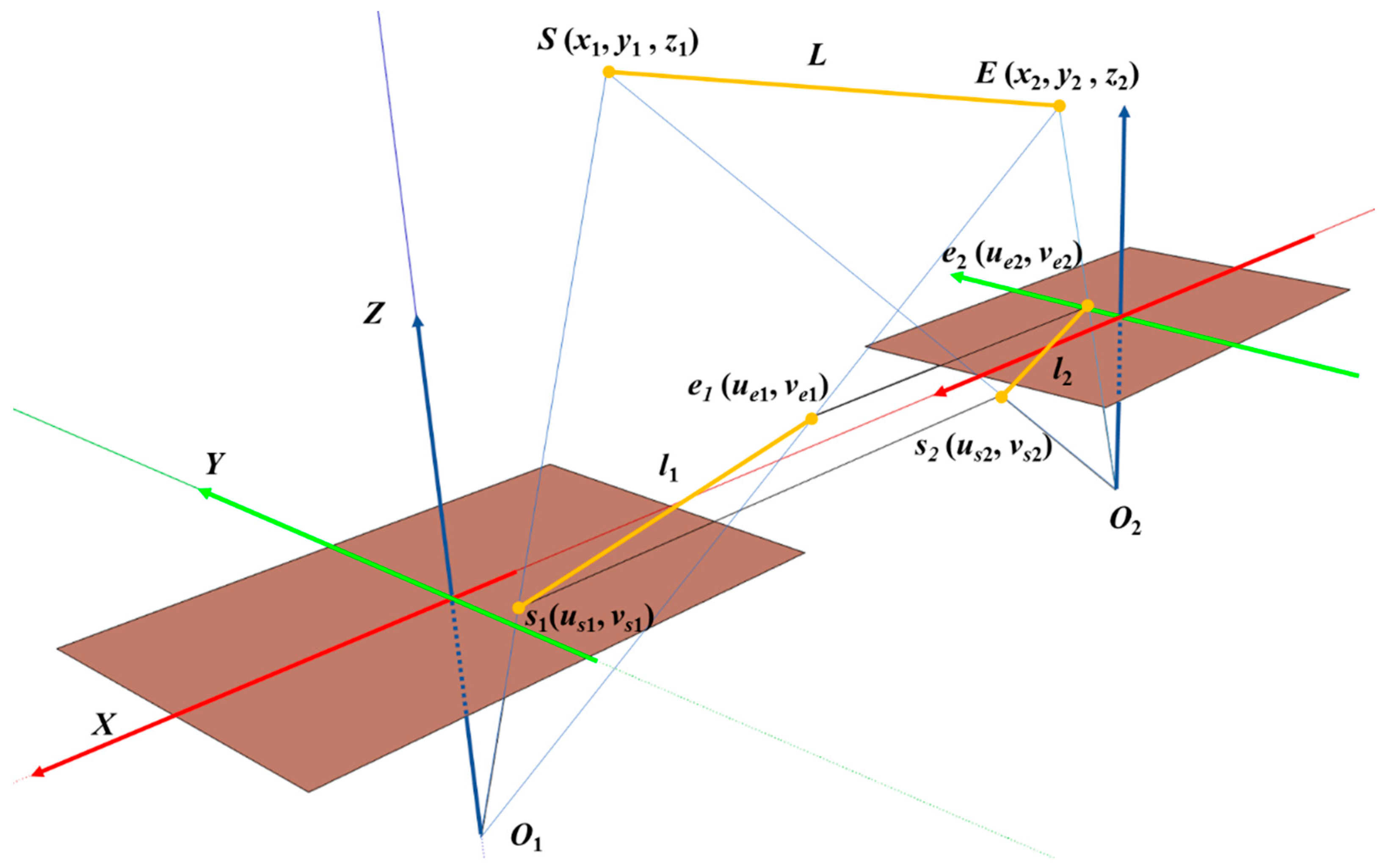
Since a three-dimensional straight line can be initialized by two points in its space, as shown in Figure 2, we set the coordinates of their two endpoints as S = ( x 1 , y 1 , z 1 ) T , E = ( x 2 , y 2 , z 2 ) T . Then, the Plücker coordinates of the straight line in space can be expressed as:
L = [ S × E S E ] = [ n v ] 6    
where n 3 is the normal vector of the plane determined by the line and the origin, and v 3 is the direction vector of the line.
Corresponding to the triangulation processing of feature points, the triangulation of line segments is used in visual odometry to add line segments to map landmarks to realize multi-element feature landmarks. Let the plane line segments corresponding to the space straight line L on the two images be l1 and l2, respectively, then:
l 1 = ( s 1 , e 1 )
l 2 = ( s 2 , e 2 )
The starting point of line segment l1 is s 1 ( u s 1 , v s 1 ) , the ending point is e 1 ( u e 1 , v e 1 ) , the starting point of line segment l2 is s 2 ( u s 2 , v s 2 ) , and the ending point is e 2 ( u e 2 , v e 2 ) . The intersection line between the plane determined by the camera optical center position O1 and the line segment l1 in the image I1 and the plane determined by the next camera position optical center O2 and the line segment l2 in the image I2 is the spatial coordinate position of the straight line.
According to the basic principle of the space plane equation, the equation of the plane πi is set as A i x + B i y + C i z = D i , a plane is uniquely determined by 3 points, and the plane equation πi determined by the camera optical center Oi and the line segment endpoint si, ei can be obtained using the following two formulas:
[ A i B i C i ] = [ s i ] × e i
D i = [ A i B i C i ] [ x i y i z i ]
Of these, [ ] × represents the antisymmetric matrix of the vector. The plane π1(O1, s1, e1) and π2(O2, s2, e2) are obtained by the above two formulas, then the spatial linear coordinates can be obtained according to the dual Plücker matrix:
L w = [ [ v w ] × n w n w T 0 ] = π 1 π 2 T π 2 π 1 T 4
Let T c w S E ( 3 ) be the transformation from the world coordinate system to the camera coordinate system, which consists of a rotation transformation R c w S O ( 3 ) and a translation t c w 3 . The transformation process of the space straight line L w from the coordinates of the world coordinate system to the coordinates of the camera coordinate system L c is shown in the following formula:
T c w = [ R c w t c w 0 1 ]
L c = [ n c v c ] = H c w L w = [ R c w [ t c w ] × R c w 0 R c w ] L w
The representation of the space line in the camera coordinate system, the process of projecting L c onto the image plane is shown in the following formula:
l = K n c = [ f y 0 0 0 f x 0 f y c x f x c y f x f y ] n c
Of these, K represents the projection matrix of the line. Because there are mismatches and matching deviations in the matching of line segments, we propose a geometric constraint method for line segments. As shown in Figure 2, according to the projection process of Formula (9), the space straight line L corresponding to the projection line segments on the two pictures is l1 and l2, respectively. According to the triangular geometric relationship, the line connecting the endpoints of the projected line segments l1 and l2 has the constraint of a parallel relationship; the analytical description is as follows:
l 1 = K n c 1
l 2 = K n c 2 = K [ R c 2 c 1 [ t c 2 c 1 ] × R c 2 c 1 ] n c 1
Among them, R c 2 c 1 and t c 2 c 1 represent the rotation and translation from camera 1 to camera 2, respectively, obtained from Formulas (10) and (11):
n c 2 = [ R c 2 c 1 [ t c 2 c 1 ] × R c 2 c 1 ] n c 1
[ t c 2 c 1 ] × n c 2 = [ [ t c 2 c 1 ] × R c 2 c 1 [ t c 2 c 1 ] × [ t c 2 c 1 ] × R c 2 c 1 ] n c 1
Since t c 2 c 1 and t c 2 c 1 are parallel vectors, the outer product of parallel vectors is 0, so there are:
[ t c 2 c 1 ] × n c 2 = [ t c 2 c 1 ] × R c 2 c 1 n c 1
Multiply both sides of the equal sign by n c 2 T at the same time:
n c 2 T [ t c 2 c 1 ] × n c 2 = n c 2 T [ t c 2 c 1 ] × R c 2 c 1 n c 1
Since n c 2 T and [ t c 2 c 1 ] × n c 2 are perpendicular to each other, there are:
n c 2 T [ t c 2 c 1 ] × R c 2 c 1 n c 1 = 0
Therefore, the line segments l1 and l2 satisfy the geometric constraints determined by the above formula.
The straight line in space has four degrees of freedom, and Plücker parameterization requires six parameters to represent the straight line, which leads to over-parameterization. This requires constrained optimization, creating further difficulties. We use these two parameterization forms in the SLAM system at the same time and use Plücker coordinates when initializing and performing space transformation. In the back-end graph optimization, the extra degrees of freedom will increase the computational cost and cause numerical instability. Therefore, the smallest four-parameter orthonormal representation is used. The orthogonal representation (R, D)∈SO(3) × SO(2) can be obtained from the Plücker coordinates:
L = [ n | v ] = [ n n v v n × v n × v ] [ n 0 0 v 0 0 ] = R [ t 1 0 0 t 2 0 0 ] .
Further, the orthonormal representation of straight line L = ( R , D ) is:
R = R ( θ ) = [ r 11 r 12 r 13 r 21 r 22 r 23 r 31 r 32 r 33 ] D = D ( d ) = [ t 1 t 2 t 2 t 1 ] .
We use the least four parameters L = [ θ T , d ] T 4 orthonormal to represent a straight line, update R with vector θ 3 to represent the direction of the straight line, and update D with d representing the distance from the straight line to the coordinate origin.

3.3. A Priori Dynamic Object Static

For the prior staticization of dynamic objects, we begin by detecting and describing the point-line features of non-priority dynamic objects. At the same time, we obtain the point-line features on the prior dynamic objects generated via instance segmentation and calculate the descriptors of point-line features. Then, we match the point-line features of the non-priority dynamic object to obtain the matching pairs of point-line features of the non-priority object region. Additionally, by adopting the random sampling consensus algorithm, the fundamental matrix is solved by using the point-line feature matching pairs of the non-priority dynamic object area.
Descriptor matching is performed on the point-line features of the prior dynamic object area, and a matching pair of point-line features located on the prior dynamic object area is obtained. Finally, we iteratively calculate each prior dynamic object and obtain the average value of the reprojection error of the fundamental matrix. If the average value is less than the threshold, it is a static object. The algorithm processing method used to determine the static object is shown in Algorithm 1.
Algorithm 1: A priori dynamic object static
Input: A priori dynamic object set, D; camera 1 point-line features P1, L1 and descriptors; camera 2 point-line features P2, L2 and descriptors;
Output: The static object set, S;
1 Obtain matching keypoints and matching keylines in non-priority dynamic object regions;
2 Calculate the fundamental matrix F = K T [ t ] × R K 1 ;
3  Matching keypoints and keylines for a priori dynamic object regions are extracted;
4 for each dynamic object Oi do
5 for each keypoint matching pair p i , p i do
6 Calculate keypoint matching pair error d ( p i , p i ) = | p i F ( p i ) T | X p i 2 + Y p i 2 , where X p i , Y p i
denote coordinates of epipolar line vector;
7 end for
8 for each keyline matching pair l i , l i do
9 Calculate keyline matching pair error d ( l i , l i ) = [ s T i l i l 1 2 + l 2 2 , e T i l i l 1 2 + l 2 2 ] , among them, s and e are the start point and end point of the line segment, and l1 and l2 are the coefficients of the line segment;
10 end for
11 if 1 n d ( p i , p i ) < 1 and 1 m d ( l i , l i ) < 1 then
12 Append Oi to S;
13 end if
14 end for

3.4. Dynamic Noise Tracking

The accuracy of SLAM positioning and mapping is sharply reduced due to the scattering of moving object features. To tackle this, a Bayesian fusion algorithm model oriented to semantics and point-line constraints is adopted. As shown in Figure 3, firstly, the convolutional neural network Mask-RCNN instance segmentation method is used to obtain a priori potential dynamic region masks. Then, a priori dynamic object contours are obtained using masks. Second, according to the outline, the point-line features at the edge are obtained. Finally, Bayesian theory is used for information fusion for semantic mask contours to obtain the dynamic probability of object features and realize dynamic tracking of edge features, which is used to solve the problem of sharp decline in the accuracy of SLAM positioning and mapping caused by dynamic object feature scattering.
The distance from feature fi to segmentation boundary b is defined as:
dist ( f i , b ) = m i n f i b 2
where b is the object segmentation edge, and the coordinates are expressed as pixel coordinates.
A meta-logistic regression model is defined to estimate the semantically dynamic segmentation probability of feature fi:
P ( D k ( f i ) s m a s k ) = 1 exp ( dist ( f i , b j ) )
The dynamic probability of semantics means that the closer the point-line feature near the mask is to the edge, the higher the probability of misclassification. Therefore, if a feature fi has an unusually high probability, it is more likely to be a dynamic feature despite being outside the mask.
Based on Bayesian theory, the state of the matched feature pi in the current frame is defined as D k ( f i ) . If the feature fi is in the region of the moving object, it is considered a dynamic feature; then, D k ( f i ) = 1 . Others are treated as static: D k ( f i ) = 0 . The movement probability of the feature in the history frame is used as the prior probability. Then, the posterior probability is expressed as:
P ( D k ( f i ) = 1 ( D k ( f i ) s m a s k ) ) = P ( D k 1 ( f i ) = 1 ) P ( ( D k ( f i ) s m a s k ) D k 1 ( f i ) = 1 ) P ( D k ( f i ) s m a s k )
The semantic dynamic probability, that is, the observation probability, is P ( D k ( f i ) s m a s k ) . Then, using the observation probability ( D k ( f i ) s m a s k ) and the prior probability P ( D k 1 ( f i ) = 1 ) , as well as the current movement probability P ( D k ( f i ) = 1 ) , are updated. The features with high moving probability are regarded as dynamic features, and the tracking of dynamic map features is eliminated to realize a robust SLAM algorithm system.
The algorithm processing method used for dynamic noise tracking to eliminate outliers is shown in Algorithm 2. The input of the algorithm is the prior dynamic object mask and the map feature, and the output is the interior point and the dynamic probability, which is used to realize dynamic denoising.
Algorithm 2: Outlier elimination algorithm of dynamic noise tracking
Input: Priori dynamic object masks, M and map features f;
Output: Inlier and dynamic probability set, F;
1 Obtain priori dynamic object contours using masks M, b;
2 for each feature fi do
3 Calculate the distance from feature fi to segmentation boundary b, dist ( f i , b ) = m i n f i b 2 ;
4 Estimate the semantically dynamic segmentation probability of feature fi:
P ( D k ( f i ) s m a s k ) = 1 exp ( dist ( f i , b j ) ) ;
5 Calculate the posterior probability P ( D k ( f i ) = 1 ( D k ( f i ) s m a s k ) ) = P ( D k 1 ( f i ) = 1 ) P ( ( D k ( f i ) s m a s k ) D k 1 ( f i ) = 1 ) P ( D k ( f i ) s m a s k ) ;
6 using the observation probability ( D k ( f i ) s m a s k ) and the prior probability P ( D k 1 ( f i ) = 1 ) , update the current movement probability P ( D k ( f i ) = 1 ) ;
7 if   P ( D k ( f i ) = 1 )   then
8 Append fi to F;
9  end if
10 end for

3.5. Optimize Error Function Construction

Let us assume a keyframe’s keypoint ui and a map point Pi are the same points. The map point measurement error Epoints refers to the difference between the keypoint ui in the current image and the corresponding point projected from the map point Pi to the image. According to the standard feature point-based SLAM three-dimensional point re-shooting error [30], the point measurement error is:
E points = k K ( u i , P i ) X p k { u i π ( T c w ( P i ) ) } T Σ 1 { u i π ( T c w ( P i ) ) }
Among them, X p k represents the set of all keypoint matches in the kth keyframe, π is the projection transformation, and T c w is the transformation matrix from the world coordinate system to the camera coordinate system. According to the projection equation of Formulas (8) and (9), the projection of the space straight line on the image plane is l, then:
l = K n c = [ l 1 l 2 l 3 ]
Therefore, the reprojection error e l between the matching line segment l and the projected line segment l in the image is expressed as:
E l i n e s = k K ( l i , l i ) Y l k d ( l i , l i ) = k K ( l i , l i ) Y l k [ s T i l i l 1 2 + l 2 2 , e T i l i l 1 2 + l 2 2 ] T
where, s i ( u s , v s ) and e i ( u e , v e ) represent the starting point and the ending point of the line segment li in the image plane, respectively.
The objective function of the corresponding point line feature is as follows:
E s u m = argmin E i K [ j P e i j Σ e i j 1 e i j + k L e i k Σ e i k 1 e i k ]
Among them, Σ e i j 1 and Σ e i k 1 are information matrices.

4. Experimental Results

To verify the proposed PLDS-SLAM system, in this section, we present some experimental details. To test and analyze the proposed PLDS-SLAM, we conduct experimental tests using an Intel i9-7900X CPU @ 3.30GHz×20, 64GB RAM, and 2080TIGPU. The proposed PLDS-SLAM algorithm is compared with the state-of-the-art ORB-SLAM2 [5] and PL-SLAM [13]. In the HPSequences dataset [31] and the KITTI stereo dataset [32], which provides challenging dynamic environment image sequences, comparative experiments on line segment matching, object static geometric constraints, dynamic object feature tracking, and trajectory measurement are carried out. Additionally, we use the EVO [33] evaluation tool to evaluate the absolute trajectory error between the estimated value of the SLAM system and the real value given by the data set. Through experimental comparison, the effectiveness of our proposed method is demonstrated.

4.1. Line Feature Matching Geometry Constraint Improvements

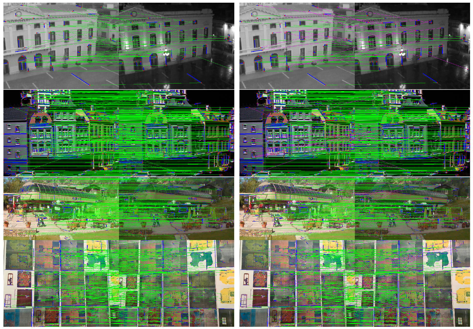
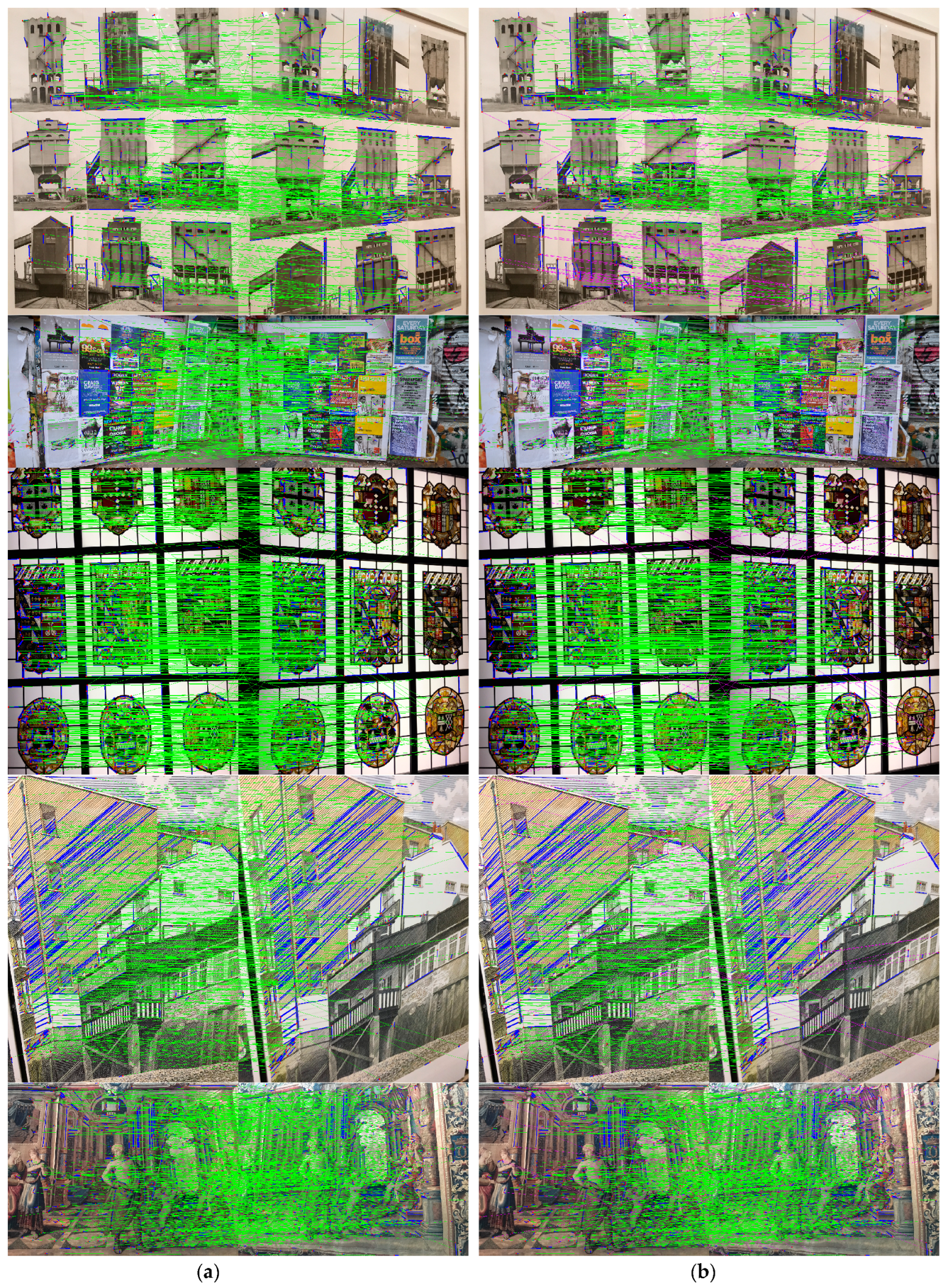
In this work, the comparison experiments of improved line matching and unimproved line matching are performed to determine the effects on the lighting and viewing angle. The comparison experiment results are shown in Figure 4. From the experimental results, compared with the matching results without geometric constraints, it can be seen that the line-matching results after geometric constraints effectively filter out the wrong matches. The effectiveness of the proposed method in line matching is demonstrated. We have added a table to compare the total matched line segments, reprojection error of k-nearest neighbor matching, and reprojection error results of our proposed method, as shown in Table 1. The bold font in the table represents the optimal result. From the experimental results in Table 1, we can see that our proposed method can effectively remove outliers in line segments, reduce the reprojection error of matching, and thus improve the accuracy and precision of line segment matching.
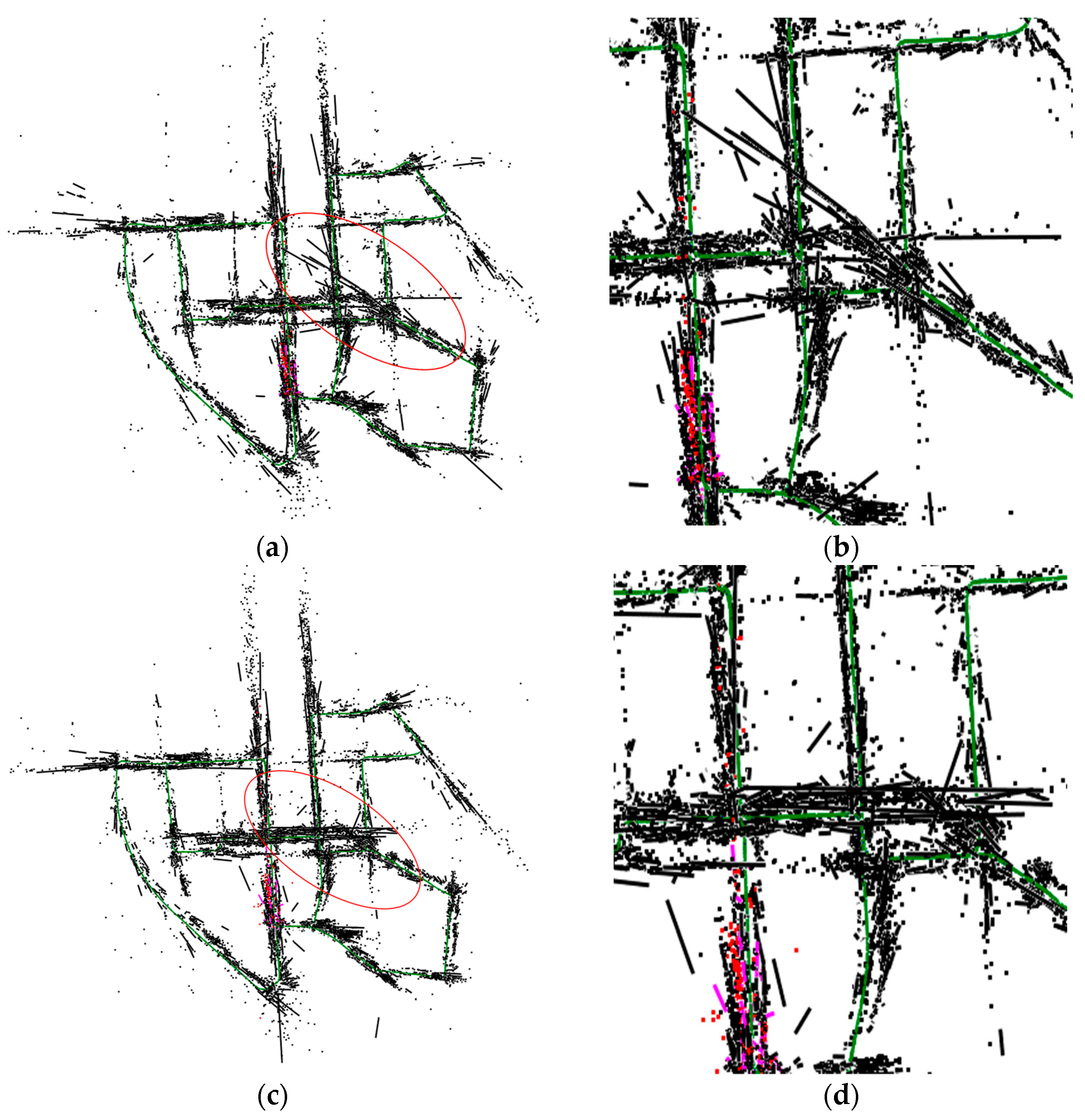
In addition, we also compare the point-line feature maps before and after geometric constraints on the KITTI dataset. As shown in Figure 5, in the comparison results of Figure 5a–d, such as the local detail map marked by the ellipse in the figure, it can be seen that geometric constraints can effectively filter out some erroneous line segment map features. The proposed method in filtering out-of-line segments can be concluded based on the experimental results.

4.2. Dynamic Noise Removal Experiment

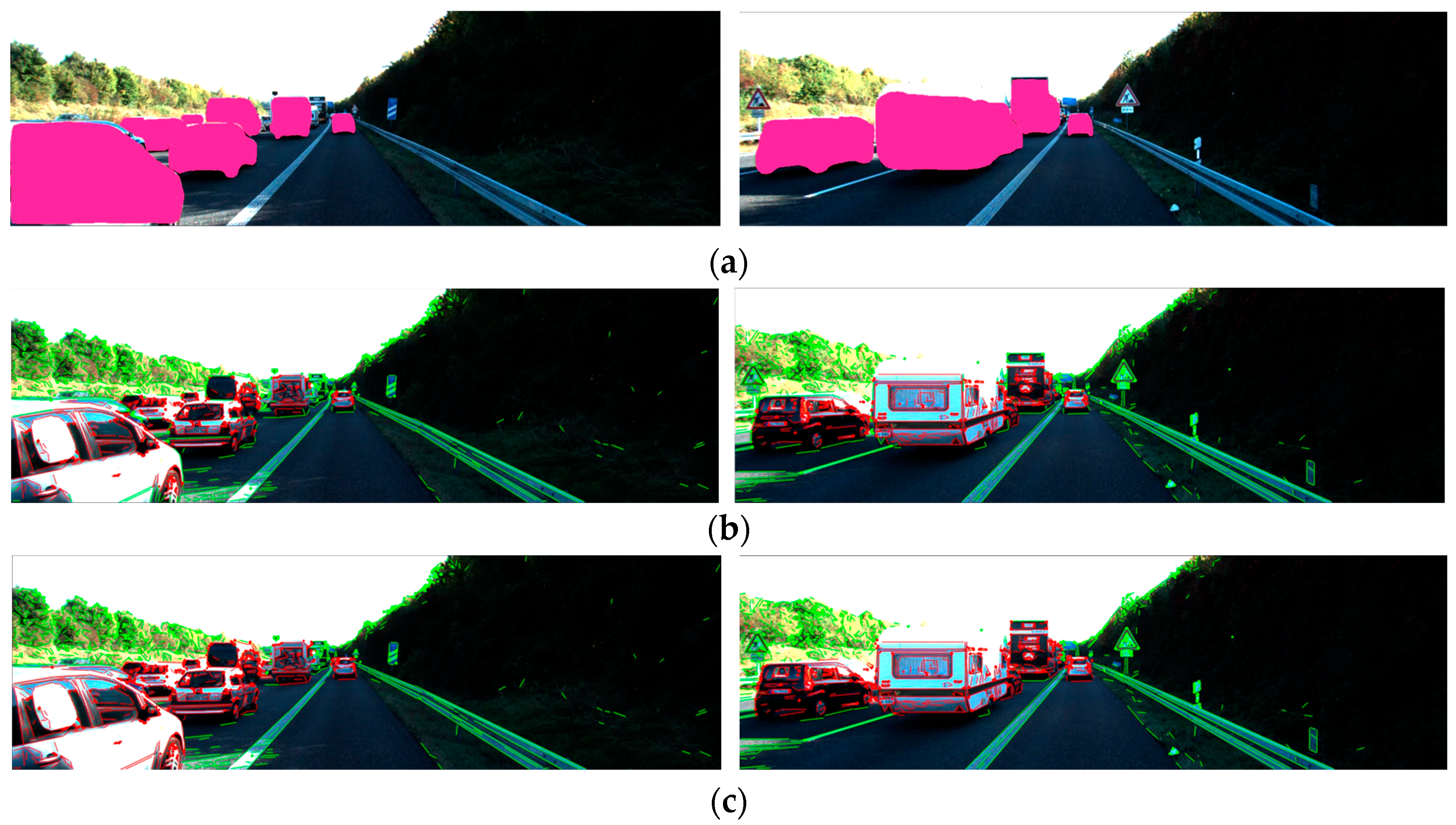
In this part of the experiment, we first use mask-RCNN to segment the input image to determine the priority of the dynamic object, obtain the contour boundary of the prior dynamic object, and we perform Bayesian dynamic feature tracking on the point line features near the boundary, which is known as dynamic tracking. The comparison results before and after are shown in Figure 6. Figure 6a is the object segmentation masks, where the pink area is the prior dynamic object segmentation result. Figure 6b shows the experimental results of point-line feature detection without tracking the edge of the dynamic object, where the red point and line is the feature on the prior dynamic object, and the green point and line is the feature of the non-dynamic prior area. Figure 6c is the result of tracking the edge point and line features of the dynamic object. From the comparison results of the point-line features of the object edge in Figure 6b,c, it can be seen that the classification of the edge dynamic point-line features after dynamic probability tracking is more accurate. In addition, as shown in Figure 7a,b, we counted the number of points and line features and the number of dynamic noise points and line features, respectively. The experimental results demonstrate that our proposed method can effectively remove dynamic point-line feature noise; the experimental results also demonstrate the effectiveness of the method in line matching.

4.3. Dynamic and Static Object Feature Separation

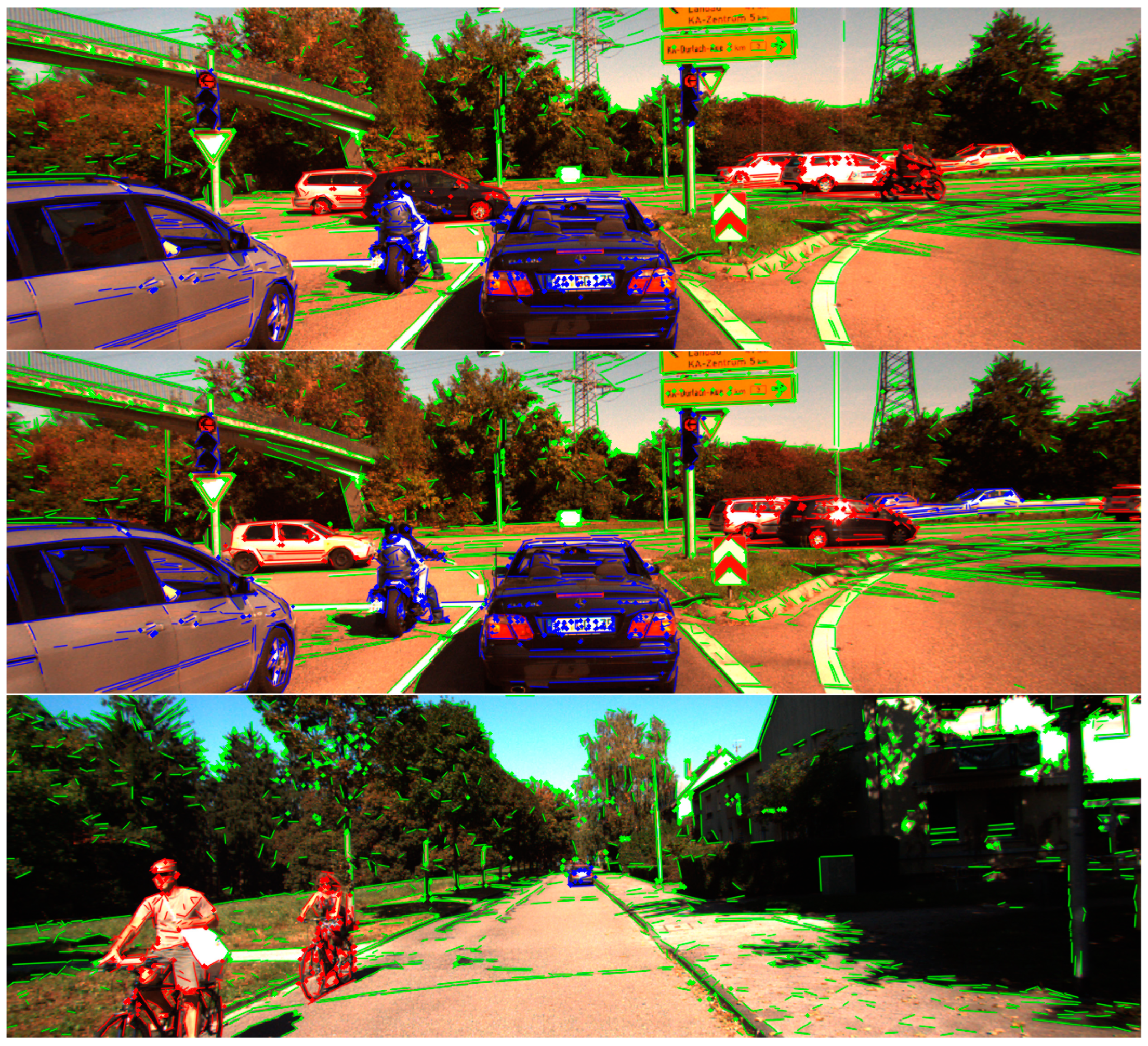
In this section, we conduct experiments on the separation of dynamic object features and static object features. As shown in Figure 8, the red point and line feature are the separated dynamic object features, and the blue point and line are the separated static object features. The experimental results show that the proposed method effectively separates the highly dynamic car object features and the static car object features, which proves the effectiveness of the proposed method.

4.4. Dynamic Environment Trajectory Accuracy Verification Experiment

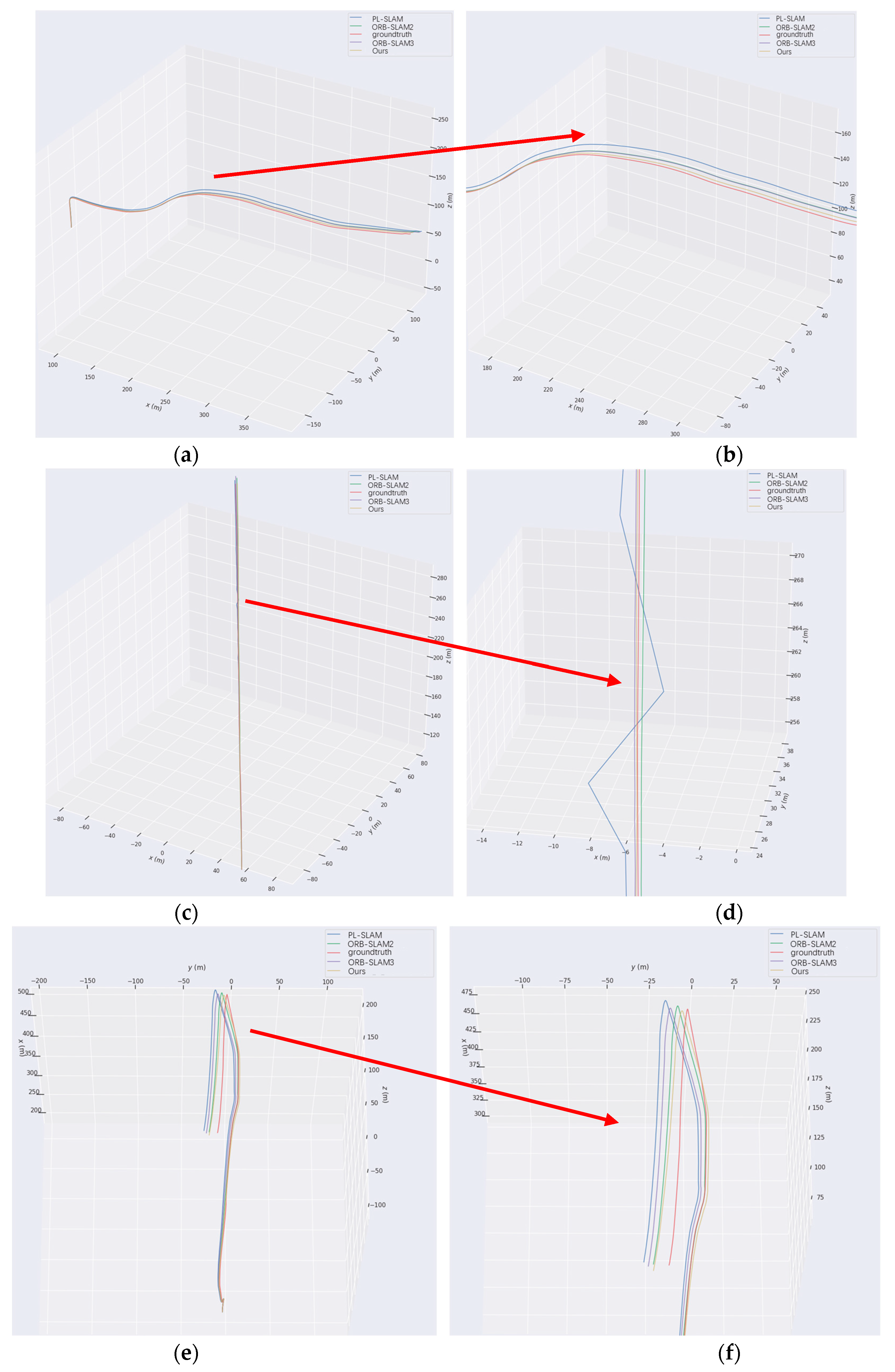
In this part, we compared the proposed method with the excellent feature point-based ORB-SLAM2, ORB-SLAM3 and the excellent point-line feature-based PL-SLAM on the KITTI dataset. To demonstrate the effectiveness of our proposed method on dynamic datasets, we conducted comparative experiments on sequence 03, sequence 04, and sequence 10 of the KITTI dataset, which contain typical dynamic scenes. As shown in Figure 9a–f from the global map and the large map that our proposed method has the smallest error with the ground truth distance compared with ORB-SLAM2, ORB-SLAM3, and PL-SLAM. This highlights the superior performance of our proposed method on dynamic datasets.
We conducted comparative experiments on the absolute trajectory errors of our proposed method and the ORB-SLAM2, ORB-SLAM3, and PL-SLAM algorithms on the dynamic dataset. Table 2 shows the absolute trajectory accuracy errors of these algorithms, where the bold ones are the optimal results. Based on the experimental results, it can be seen that the accuracy of our proposed method is better than that of ORB-SLAM2, ORB-SLAM3, and PL-SLAM methods on dynamic datasets.

5. Conclusions

In this paper, we explore the multi-element coupling mechanism of semantics and multi-view geometric features in a dynamic environment and propose a new stereo point-line SLAM system based on a dynamic environment. Our method obtains a priori dynamic region features by detecting and segmenting the dynamic region. It also proposes a geometric constraint method for matching line segments, and it combines the pole-constrained method of point features to separate dynamic and static objects. The dynamic feature tracking method based on Bayesian eliminates outliers to improve the robustness and accuracy of the SLAM system. The effectiveness of our proposed method in dynamic scenes is demonstrated by comparative experiments on the KITTI dataset and HPSequences dataset.

Author Contributions

Conceptualization, Y.X.; methodology, C.Y.; formal analysis, C.Y.; investigation, C.Y.; resources, Q.Z.; writing—original draft preparation, C.Y.; visualization, Q.Z.; supervision, Y.X.; project administration, Y.X. All authors have read and agreed to the published version of the manuscript.

Funding

This research is supported by The Nature Science Foundation of Shaanxi under Grant 2022JQ-653 and The Fundamental Research Funds for the Central Universities, Northwestern Polytechnical University (No. D5000210767).

Data Availability Statement

Not applicable.

Conflicts of Interest

The authors declare no conflict of interest.

References

  1. Davison, A.J. Real-time simultaneous localisation and mapping with a single camera. In Computer Vision, Proceedings of the IEEE International Conference on IEEE Computer Society, Nice, France, 13–16 October 2003; Department of Engineering Science, University of Oxford: Oxford, UK, 2003; Volume 3, p. 1403. [Google Scholar]
  2. Klein, G.; Murray, D. Parallel tracking and mapping for small AR workspaces. In Proceedings of the 2007 6th IEEE and ACM International Symposium on Mixed and Augmented Reality, Nara, Japan, 13–16 November 2007; IEEE: New York, NY, USA; pp. 225–234. [Google Scholar]
  3. Bartoli, A.; Sturm, P. Structure-from-motion using lines: Representation, triangulation, and bundle adjustment. Comput. Vis. Image Underst. 2005, 100, 416–441. [Google Scholar] [CrossRef] [Green Version]
  4. Mur-Artal, R.; Montiel, J.M.M.; Tardos, J.D. ORB-SLAM: A versatile and accurate monocular SLAM system. IEEE Trans. Robot. 2015, 31, 1147–1163. [Google Scholar] [CrossRef] [Green Version]
  5. Mur-Artal, R.; Tardós, J.D. Orb-slam2: An open-source slam system for monocular, stereo, and rgb-d cameras. IEEE Trans. Robot. 2017, 33, 1255–1262. [Google Scholar] [CrossRef] [Green Version]
  6. Gálvez-López, D.; Tardos, J.D. Bags of binary words for fast place recognition in image sequences. IEEE Trans. Robot. 2012, 28, 1188–1197. [Google Scholar] [CrossRef]
  7. Campos, C.; Elvira, R.; Rodriguez, J.J.G.; Montiel, J.M.M.; Tardos, J.D. ORB-SLAM3: An Accurate Open-Source Library for Visual, Visual–Inertial, and Multimap SLAM. IEEE Trans. Robot. 2021, 37, 1874–1890. [Google Scholar] [CrossRef]
  8. Engel, J.; Schöps, T.; Cremers, D. LSD-SLAM: Large-scale direct monocular SLAM. In Proceedings of the European Conference on Computer Vision, Zurich, Switzerland, 6–12 September 2014; Springer: Cham, Switzerland, 2014; pp. 834–849. [Google Scholar]
  9. Forster, C.; Pizzoli, M.; Scaramuzza, D. SVO: Fast semi-direct monocular visual odometry. In Proceedings of the 2014 IEEE International Conference on Robotics and Automation (ICRA), Hong Kong, China, 31 May–7 June 2014; IEEE: New York, NY, USA, 2014; pp. 15–22. [Google Scholar]
  10. Engel, J.; Koltun, V.; Cremers, D. Direct sparse odometry. IEEE Trans. Pattern Anal. Mach. Intell. 2017, 40, 611–625. [Google Scholar] [CrossRef]
  11. Rong, H.; Gao, Y.; Guan, L.; Ramirez-Serrano, A.; Xu, X.; Zhu, Y. Point-Line Visual Stereo SLAM Using EDlines and PL-BoW. Remote Sens. 2021, 13, 3591. [Google Scholar] [CrossRef]
  12. Akinlar, C.; Cihan, T. EDLines: A real-time line segment detector with a false detection control. Pattern Recognit. Lett. 2011, 32, 1633–1642. [Google Scholar] [CrossRef]
  13. Gomez-Ojeda, R.; Moreno, F.; Scaramuzza, D.; Gonzalez-Jimenez, J. PL-SLAM: A stereo SLAM system through the combination of points and line segments. IEEE Trans. Robot. 2019, 35, 734–746. [Google Scholar] [CrossRef] [Green Version]
  14. Zuo, X.; Xie, X.; Liu, Y.; Huang, G. Robust visual SLAM with point and line features. In Proceedings of the 2017 IEEE/RSJ International Conference on Intelligent Robots and Systems (IROS), Vancouver, BC, Canada, 24–28 September 2017; IEEE: New York, NY, USA, 2017. [Google Scholar]
  15. Kim, D.H.; Kim, J.H. Effective background model-based RGB-D dense visual odometry in a dynamic environment. IEEE Trans. Robot. 2016, 32, 1565–1573. [Google Scholar] [CrossRef]
  16. Li, S.; Lee, D. RGB-D SLAM in dynamic environments using static point weighting. IEEE Robot. Autom. Lett. 2017, 2, 2263–2270. [Google Scholar] [CrossRef]
  17. Sun, Y.; Liu, M.; Meng, M.Q.H. Motion removal for reliable RGB-D SLAM in dynamic environments. Robot. Auton. Syst. 2018, 108, 115–128. [Google Scholar] [CrossRef]
  18. Scona, R.; Jaimez, M.; Petillot, Y.R.; Fallon, M.; Cremers, D. Staticfusion: Background reconstruction for dense rgb-d slam in dynamic environments. In Proceedings of the 2018 IEEE International Conference on Robotics and Automation (ICRA), Brisbane, Australia, 21–25 May 2018; IEEE: New York, NY, USA, 2018; pp. 3849–3856. [Google Scholar]
  19. Dai, W.; Zhang, Y.; Li, P.; Fang, Z.; Scherer, S. Rgb-d slam in dynamic environments using point correlations. IEEE Trans. Pattern Anal. Mach. Intell. 2020, 44, 373–389. [Google Scholar] [CrossRef] [PubMed]
  20. Zhang, Z.; Doi, K.; Iwasaki, A.; Xu, G. Unsupervised Domain Adaptation of High-Resolution Aerial Images via Correlation Alignment and Self Training. IEEE Geosci. Remote Sens. Lett. 2020, 18, 746–750. [Google Scholar] [CrossRef]
  21. Zhang, Z.; Ji, A.; Wang, K.; Zhang, L. UnrollingNet: An attention-based deep learning approach for the segmentation of large-scale point clouds of tunnels. Autom. Constr. 2022, 142, 104456. [Google Scholar] [CrossRef]
  22. Yu, C.; Liu, Z.; Liu, X.J.; Xie, F.; Yang, Y.; Wei, Q.; Fei, Q. DS-SLAM: A semantic visual SLAM towards dynamic environments. In Proceedings of the 2018 IEEE/RSJ International Conference on Intelligent Robots and Systems (IROS), Madrid, Spain, 1–5 October 2018; IEEE: New York, NY, USA, 2018; pp. 1168–1174. [Google Scholar]
  23. Badrinarayanan, V.; Kendall, A.; Cipolla, R. Segnet: A deep convolutional encoder-decoder architecture for image segmentation. IEEE Trans. Pattern Anal. Mach. Intell. 2017, 39, 2481–2495. [Google Scholar] [CrossRef]
  24. Bescos, B.; Fácil, J.M.; Civera, J.; Neira, J. DynaSLAM: Tracking, mapping, and inpainting in dynamic scenes. IEEE Robot. Autom. Lett. 2018, 3, 4076–4083. [Google Scholar] [CrossRef] [Green Version]
  25. Lin, T.Y.; Goyal, P.; Girshick, R.; He, K.; Dollár, P. Mask r-cnn. In Proceedings of the IEEE International Conference on Computer Vision, Venice, Italy, 22–29 October 2017; pp. 2961–2969. [Google Scholar]
  26. Zhang, J.; Henein, M.; Mahony, R.; Ila, V. VDO-SLAM: A visual dynamic object-aware SLAM system. arXiv 2020, arXiv:2005.11052. [Google Scholar]
  27. Li, A.; Wang, J.; Xu, M.; Chen, Z. DP-SLAM: A visual SLAM with moving probability towards dynamic environments. Inf. Sci. 2021, 556, 128–142. [Google Scholar] [CrossRef]
  28. Von Gioi, R.G.; Jakubowicz, J.; Morel, J.M.; Randall, G. LSD: A line segment detector. Image Process. Line 2012, 2, 35–55. [Google Scholar] [CrossRef] [Green Version]
  29. Zhang, L.; Reinhard, K. An efficient and robust line segment matching approach based on LBD descriptor and pairwise geometric consistency. J. Vis. Commun. Image Represent. 2013, 24, 794–805. [Google Scholar] [CrossRef]
  30. Saputra, M.R.U.; De Gusmao, P.P.; Wang, S.; Markham, A.; Trigoni, N. Learning monocular visual odometry through geometry-aware curriculum learning. In Proceedings of the 2019 International Conference on Robotics and Automation (ICRA), Montreal, QC, Canada, 20–24 May 2019; IEEE: New York, NY, USA, 2019; pp. 3549–3555. [Google Scholar]
  31. Balntas, V.; Lenc, K.; Vedaldi, A.; Tuytelaars, T.; Matas, J.; Mikolajczyk, K. HPatches: A benchmark and evaluation of handcrafted and learned local descriptors. In Proceedings of the IEEE Conference on Computer Vision and Pattern Recognition, Honolulu, HI, USA, 21–26 July 2017. [Google Scholar]
  32. Geiger, A.; Lenz, P.; Urtasun, R. Are we ready for autonomous driving? The KITTI vision benchmark suite. In Proceedings of the 2012 IEEE Conference on Computer Vision and Pattern Recognition (CVPR), Providence, RI, USA, 16–21 June 2012; pp. 3354–3361. [Google Scholar]
  33. Grupp, M. evo: Python package for the evaluation of odometry and slam. Search 2017. [Google Scholar]
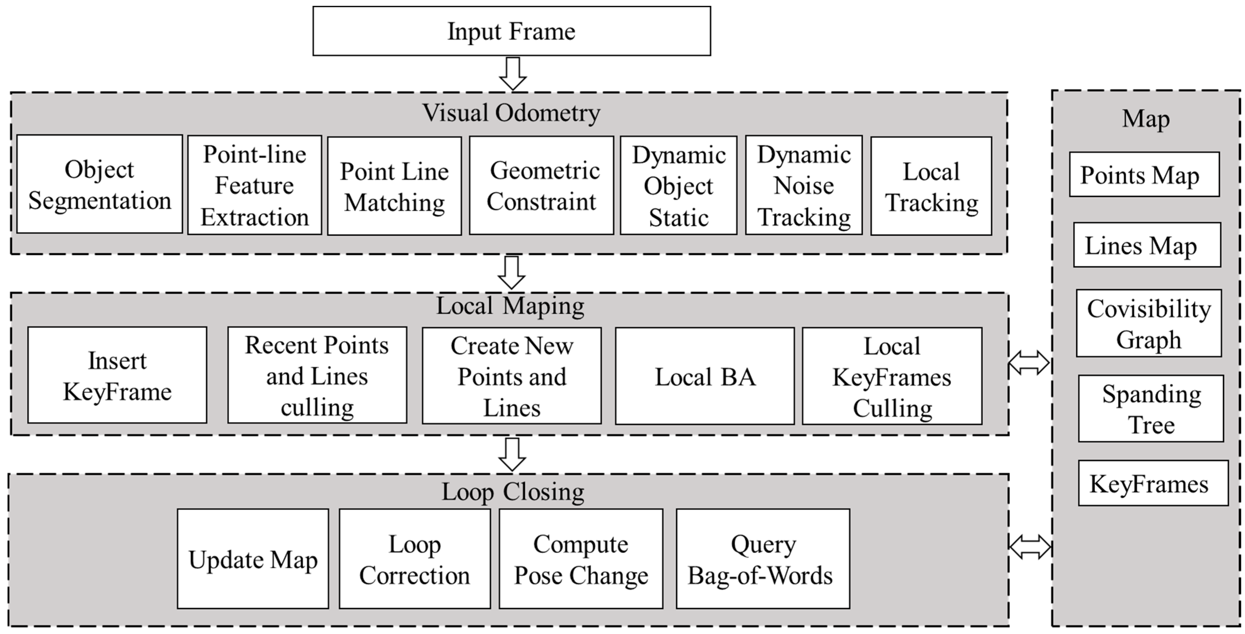
Figure 1. Block diagram of PLDS-SLAM algorithm based on point-line features.
Remotesensing 15 01893 g001
Figure 2. Space line projection and geometric constraint relationship.
Remotesensing 15 01893 g002
Figure 3. Flow chart of dynamic tracking and extraction of object point and line features.
Remotesensing 15 01893 g003
Figure 4. Comparison of line segment matching results before and after geometric constraints. Among them, the green connection line represents the matching correspondence, the pink connection line is the mismatching correspondence, the blue connection line is the matching line segment, and the red point is the endpoint of the connected corresponding line segment. (a) Matching before geometric constraints. (b) Matching after geometric constraints.
Remotesensing 15 01893 g004aRemotesensing 15 01893 g004b
Figure 5. Comparison of point-line graphs before and after geometric constraints, where the green line is the camera movement trajectory, the black dot line is the point-line graph, the red point is the point feature seen by the SLAM system from the current perspective, and the pink line is the current perspective of the SLAM system line features. (a,b) show the global and local point-line feature maps, respectively, before applying geometric constraints, while (c,d) show the global and local point-line feature maps, respectively, after applying geometric constraints. The local point-line feature map and trajectory correspond to the red ellipse area in the global map., in which the local point-line feature map and the trajectory corresponding to the red ellipse area in the global map. (a) Global point-line map and trajectory. (b) Local point-line map and trajectory. (c) Global point-line map and trajectory. (d) Local point-line map and trajectory.
Remotesensing 15 01893 g005
Figure 6. Comparison of dynamic feature probability before and after tracking results. (a) Semantic segmentation masks. (b) Before dynamic tracking. (c) After dynamic probability tracking.
Remotesensing 15 01893 g006
Figure 7. Point line feature dynamic noise statistics on KITTI dataset. The horizontal coordinate represents the frame number, and the vertical coordinate represents the number of features. (a) Line Feature Dynamic Noise Statistics. (b) Point Feature Dynamic Noise Statistics.
Remotesensing 15 01893 g007
Figure 8. Dynamic object and static object separation experiment, in which the blue point and line is the static object, and the red point and line is the dynamic object.
Remotesensing 15 01893 g008
Figure 9. A comparative experiment is carried out on the KITTI dynamic data set, where the red line is the real value, the light yellow line is our proposed method, the green line is the ORB-SLAM2 method, the blue line is the PL-SLAM method, and the light blue line is the ORB-SLAM3 method. (a,b) are space estimation comparisons in the KITTI dataset sequence 03. (c,d) are spatial estimation comparisons in the KITTI dataset sequence 04. (e,f) are spatial estimations in the KITTI dataset sequence 10. Among them, (a,c,e) are spatial contrast, (b,d,f) are the comparison of details.
Remotesensing 15 01893 g009
Table 1. Outlier removal experiments of line segments.
Frame010203040506070809
Total Lines50547363419358490807405682
Projection Errors of K-Nearest Neighbors77.5716.7863.3475.3957.2362.6250.4559.5050.56
Projection Errors of Ours1.161.061.250.951.461.061.160.871.97
Table 2. Absolute trajectory error comparison on the KITTI dataset.
Dataset OursORB-SLAM2ORB-SLAM3PL-SLAM
Sequence003.5781.6971.9942.551
Sequence012.3103.2688.8472.423
Sequence023.7993.6793.6016.635
Sequence032.7402.9003.3234.410
Sequence041.1801.2601.6922.010
Sequence052.8881.7321.9612.572
Sequence062.2261.9592.1656.491
Sequence071.5790.9071.1012.211
Sequence083.9483.3503.0753.317
Sequence093.0874.2193.4114.023
Sequence102.2402.2902.2423.190
Disclaimer/Publisher’s Note: The statements, opinions and data contained in all publications are solely those of the individual author(s) and contributor(s) and not of MDPI and/or the editor(s). MDPI and/or the editor(s) disclaim responsibility for any injury to people or property resulting from any ideas, methods, instructions or products referred to in the content.