Satellite-Derived Land Surface Temperature Dynamics in the Context of Global Change—A Review

Abstract

Satellite-derived Land Surface Temperature (LST) dynamics have been increasingly used to study various geophysical processes. This review provides an extensive overview of the applications of LST in the context of global change. By filtering a selection of relevant keywords, a total of 164 articles from 14 international journals published during the last two decades were analyzed based on study location, research topic, applied sensor, spatio-temporal resolution and scale and employed analysis methods. It was revealed that China and the USA were the most studied countries and those that had the most first author affiliations. The most prominent research topic was the Surface Urban Heat Island (SUHI), while the research topics related to climate change were underrepresented. MODIS was by far the most used sensor system, followed by Landsat. A relatively small number of studies analyzed LST dynamics on a global or continental scale. The extensive use of MODIS highly determined the study periods: A majority of the studies started around the year 2000 and thus had a study period shorter than 25 years. The following suggestions were made to increase the utilization of LST time series in climate research: The prolongation of the time series by, e.g., using AVHRR LST, the better representation of LST under clouds, the comparison of LST to traditional climate change measures, such as air temperature and reanalysis variables, and the extension of the validation to heterogenous sites.

1. Introduction

1.1. Relevance of Satellite-Derived LST

Planet Earth is changing with unprecedented intensity and speed. On the one hand, there is climate change driven by anthropogenic emissions of greenhouse gases. It mainly manifests through increasing air temperature and leads to extreme weather events, changing precipitation/seasonality patterns, decreasing snow cover, glaciers and permafrost and shifting the habitats of plant and animal species. On the other hand, humans directly modify their environment through the clearing of forests, urbanization and agricultural activities. LST is a key indicator for both climate change and land surface processes, as due to the heat exchange between the land surface and the near-surface atmosphere, the dynamics in air temperature and LST are consistent [1]. Furthermore, the LST is an important parameter in surface energy balance equations and is hence crucial for understanding the dynamics in the Earth’s radiation fluxes. Therefore, LST is recognized as one of the Essential Climate Variables (ECVs) by the World Meteorological Organization. On the other side, the aforementioned land surface processes change the thermal properties of the land surface and are, therefore, also reflected in the LST.

Satellite remote sensing of LST offers the possibility to monitor climate-change-related processes spatially and continuously with high a spatial and temporal resolution, which is, e.g., not possible when using weather stations, which are unevenly distributed and only provide coarse spatial resolutions. Thermal infrared (TIR) sensors mounted on satellites are the most common source of remote-sensing-based LST. In recent decades, many satellites have been launched carrying TIR sensors, providing different spatial and temporal resolutions, e.g., the Advanced Very-High-Resolution Radiometer (AVHRR), Landsat’s Thematic Mapper (TM), Enhanced Thematic Mapper Plus (ETM+) and Thermal Infrared Sensor (TIRS), the Along Track Scanning Radiometer (ATSR), the Moderate Resolution Imaging Spectroradiometer (MODIS), the Advanced Spaceborne Thermal Emission and Reflection Radiometer (ASTER) and the Visible Infrared Imaging Radiometer Suite (VIIRS). However, most of these have been only available for the last two decades. Only Landsat and AVHRR provide a longer time series, starting from the 1980s.

In recent years, remotely sensed LST has attracted increasing interest from researchers in various fields, which is reflected by the exponentially growing number of publications in this field [1,2]. Figure 1 provides an overview of the application fields of LST. LST has been used to study global warming [3,4,5,6,7,8,9,10,11,12,13,14,15,16], interannual climate variabilities [5,7,8,9,10,14,17], heat waves [18,19,20], droughts [21,22,23,24,25], soil moisture dynamics [22,23,26,27,28,29], forest dynamics [28,30,31,32,33,34,35,36,37,38,39], general vegetation–temperature interactions [15,20,24,25,26,29,34,40,41,42,43,44,45,46,47,48,49,50,51], wildfires [28,52,53,54,55], snow and permafrost dynamics [13,16,29,56,57,58,59,60,61,62,63] and urbanization [16,51,64,65,66,67,68,69,70,71,72,73,74,75,76,77,78,79,80,81,82,83,84,85,86,87,88,89,90,91,92,93,94,95,96,97,98,99,100,101,102,103,104,105,106,107,108,109,110,111,112,113,114,115,116,117,118,119,120,121,122,123,124,125,126,127,128,129,130,131,132,133,134,135,136,137,138,139,140,141,142,143,144,145,146].

1.2. LST as Part of the Surface Energy Budget

The land surface can be defined as the interface layer between different surface components (e.g., forest canopy, rooftops and soil) and the atmosphere, and LST is its thermodynamic temperature [1]. LST is an essential part of the surface energy balance (SEB), which is depicted in Figure 2. Concerning LST, the SEB can be split into three subsystems: the shortwave radiation balance (1) [18], the longwave radiation balance (2) and the ground heat loss (3). Following this SEB model, changes in LST (ΔLST) are determined by the sum of the net shortwave radiation (R_S^net), the net longwave radiation (R_L^net) and the net ground heat loss (H^net). In the following, these three subsystems are shortly described:

(1)

The incoming shortwave radiation (R_S^down) is the portion of the solar radiation that is not absorbed or reflected by the atmosphere: that which reaches the land surface. A part of that radiation is reflected (R_S^up), while the remaining part R_S^net is absorbed by the land surface. The ratio between R_S^down, R_S^up and R_S^net is determined by the reflectivity (ρ) of the land surface and is called albedo.

(2)

The absorption of R_S^net heats up the land surface and causes it to emit longwave radiation (R_L^up) in the TIR spectrum. However, the amount of emitted longwave radiation at the same temperature can vary for different land surfaces and is determined by the emissivity (ε) of the land surface. ε is defined as the proportion of longwave radiation emitted from the respective surface relative to the amount of longwave radiation a black body would emit at the same temperature. It is an important parameter for the remote sensing of LST because TIR sensors only measure the longwave radiation, and ε has to be considered during the derivation process. R_L^TOA is the TIR longwave radiation, which is attenuated by the atmosphere and measured by the satellite sensor at the top of the atmosphere. To complete the longwave radiation budget, the incoming longwave radiation from clouds and the atmosphere also have to be considered. The difference between R_L^down and R_L^up forms the net longwave radiation (R_L^net).

(3)

In addition to indirect energy transfer via radiation, the land surface also directly exchanges heat with the adjacent atmosphere, which is called sensible heat flux (H), and with deeper ground layers, which is called ground heat flux (G₀). The third component of H^net is latent heat flux (λE), which describes the energy exchange between the land surface and atmosphere during the process of evaporation. The sum of H, G₀ and λE forms H^net and strongly depends on the absorptivity (α) of the land surface.

The SEB illustrates the main drivers of LST dynamics, which are the incoming solar radiation, the land surface spectral and thermal properties (ρ, ε and α), the incoming atmospheric radiation and the heat fluxes of the ground heat loss.

1.3. Principles of Remote Sensing of LST

As mentioned in 1.2, satellite-derived LST is measured using the thermal infrared longwave radiation at the top of the atmosphere, which is called the top-of-atmosphere brightness temperature (BT^TOA) in the context of thermal remote sensing. The right part of Figure 1 illustrates the satellite remote sensing process of LST. LST_1,2 and ε_1,2 are the emissivity integrated over all visible components of the land surface within the respective pixel. The temperature of these components can vary considerably, e.g., in urban areas; therefore, spatial resolution is a crucial factor for the remote sensing of LST. Furthermore, LST and emissivity are directional variables, wherefore the satellite zenith angle (θ_1,2) and the satellite azimuth angle φ_1,2 also have to be accounted for during the derivation of LST. The attenuation of the atmosphere is mostly driven by its water vapor content and also depends on θ and φ.

Several algorithms exist to account for emissivity and the directional and atmospheric effects in order to derive an accurate LST from satellite data. A comprehensive overview of these algorithms and their validation methods is provided by [1,147]. The validation of satellite LST should follow a certain protocol, as provided by [148]. It can either be compared to in situ LST or compared to an LST derived from other sensors, or compared to an LST modeled from radiances. The best validated LST products are derived from MODIS, reaching mean absolute deviations (MADs) of around 1 K when validated against in situ LSTs [149,150]. Other LST products have been derived from AVHRR, with MADs of around 2 K [151], and AATSR, with MADs between 1.5 and 3 K [152]. An up-to-date overview of available LST products is provided by [1]. The accordance between satellite-derived and in situ LST is usually higher at night. One general problem with most validation studies is that they are only conducted over homogenous surfaces, which does not represent well the accuracy over heterogenous surfaces, e.g., urban areas or mixed forest.

LST is not only changing rapidly in space but also in time [153]. Generally, in remote sensing, there is a tradeoff between temporal and spatial resolution, meaning that sensors providing a high temporal resolution (MODIS, AVHRR) can only provide a medium spatial resolution, while sensors providing a high spatial resolution (Landsat, ASTER) can only provide a low temporal resolution. However, in both cases, polar-orbiting satellites can only provide instantaneous LST measurements, which do not represent the daily progress of the LST. This problem is aggravated by the fact that TIR measurements cannot penetrate clouds, leading to data gaps. The LST under clouds can be reconstructed by regressing in situ LST with its determining variables as elevation, the Normalized Difference Vegetation Index (NDVI) or albedo or using Passive-Microwave-derived LST [153,154]. Another possibility is the temporal aggregation of LST to daily, weekly, monthly or annual statistics. These aggregations are established for sensors with a constant revisit time, e.g., MODIS, but these become very complex for sensors with changing revisit times over the time series, e.g., AVHRR sensors [155,156,157,158]. Furthermore, if these statistics only rely on clear-sky LSTs, they do not represent LSTs very well under cloudy conditions, which is referred to as clear-sky bias in the literature [153].

1.4. Scope and Aim of This Review

The wide interest in the remote sensing of LSTs by researchers from various fields has led to a number of reviews with different foci; however, their focus was either on LST retrieval methods [147], LST reconstruction methods [153,154], or they were dealing with specific topics (e.g., SUHI [2,159,160], such as soil moisture mapping from LSTs [161], evapotranspiration mapping from LSTs [162], the remote sensing of SEB components [163], drought indices [164] or elevation-dependent warming [165]). Recently, a comprehensive review was published by [1], which identified soil moisture estimation, agricultural drought monitoring, SUHI, thermal anomaly monitoring and climate change indices as the most common applications of LSTs. To our knowledge, there is no review yet covering the wide range of applications of satellite-derived LSTs. This paper should provide an overview of how satellite-derived LSTs are used to measure all facets of global change, bringing together applications from climate research and land surface processes for the first time. To achieve that, a systematic review of studies dealing with LST dynamics measured from satellites was conducted. Hereby, special attention was paid to studies analyzing LSTs on a temporal and spatial scale that are relevant to global change topics. The following research questions will be addressed:

• How did the research field develop over time?
• Where and on which scales have LST dynamics been analyzed?
• Which global-change-related processes have been analyzed with LST? Which are the predominant research foci?
• How applicable is LST to the study of climate change?
• Which sensors have been used?
• What temporal resolutions and scales were analyzed?
• What methods have been used to quantify LST dynamics?

Section 2 presents our review method. Section 3 presents our results with respect to the research questions above. The findings are discussed in Section 4, which is followed by a conclusion and outlook in Section 5.

2. Materials and Methods

For this review, we looked for scientific articles that were published in the last two decades and analyzed LST dynamics in order to gain knowledge of the land surface and climate processes on our planet. For our analysis, we used the Web of Science (WoS) platform. Figure 3 shows the workflow we used, which resulted in 164 reviewed publications. To match our scope, the studies should be concerned with each of the three topics: LST, satellite remote sensing and temporal dynamics resp. spatial patterns. To allow some leeway, we used several synonymous search terms for each topic:

• For the topic of LST, we included the search terms ‘lst’, ‘land surface temperature’ and ‘thermal’. To select studies concerned with satellite remote sensing, we included the terms ‘earth observation’, ‘satellite remote’, ‘rs’, ‘mapping’ and the most common thermal sensors (‘avhrr’,’aster’,’modis’,’landsat’,’aatsr’,’slstr’ and ‘viirs’). To include articles concerned with temporal dynamics or spatial patterns, we included the search terms ‘dynamic*’, ‘trend*’, ‘anomal*’, ‘multi temporal’, ‘variability’, ‘spatial pattern’ and ‘temporal pattern’. Based on these search terms and the restriction to the publication from the year 2000, our initial search returned 8416 results.
• In the second step, we limited our search to studies to the English language, document type to ‘article’ and ‘review’ and to ‘open access’ studies (n = 3728).
• After that, we limited our search to studies that matched with one of the following WoS categories: ‘Environmental Sciences’, ’Remote Sensing’, ‘Geosciences Multidisciplinary’, ‘Imaging Science Photographic Technology’, ‘Meteorology Atmospheric Sciences’, ‘Geography Physical’, ’Ecology’ and ‘Environmental Studies’, resulting in n = 2155 results.
• We further excluded all studies that were additionally assigned to a WoS category, which does not match our scope, e.g., ‘Engineering Electrical Elictronical’ or ‘Microbiology’ (n = 1616).
• Based on the resulting 1616 studies, we analyzed the associated journals. We selected 14 journals based on the number of relevant studies and the impact factor of the journal and limited our search to these journals. The selected journals are displayed in

  Table 1. List of the included journals and the corresponding count of reviewed articles.

  Journal Title	Number of Articles
  REMOTE SENSING	116
  REMOTE SENSING OF ENVIRONMENT	8
  GEOPHYSICAL RESEARCH LETTERS	6
  ENVIRONMENTAL RESEARCH LETTERS	6
  INTERNATIONAL JOURNAL OF APPLIED EARTH OBSERVATION AND GEOINFORMATION	6
  JOURNAL OF GEOPHYSICAL RESEARCH-ATMOSPHERES	5
  EGYPTIAN JOURNAL OF REMOTE SENSING AND SPACE SCIENCES	4
  FRONTIERS IN ENVIRONMENTAL SCIENCE	4
  URBAN CLIMATE	4
  JOURNAL OF CLIMATE	1
  CRYOSPHERE	1
  IEEE JOURNAL OF SELECTED TOPICS IN APPLIED EARTH OBSERVATIONS AND REMOTE SENSING	1
  ATMOSPHERE	1
  ATMOSPHERIC CHEMISTRY AND PHYSICS	1

  . The aforementioned filtering steps build up the final search string. The final search string returned 1095 results, which were exported along with all WoS Metadata, including the abstracts, and further analyzed manually.

For the manual filtering, we first looked at the study titles and excluded all of the studies that did not fit our scope. We proceeded by reading the abstracts of the remaining 273 studies. Thereby, we excluded 70 further studies and categorized the studies into one group, covering the topics of SUHI and Urbanization (n = 124) and another group covering all of the other topics (n = 79). Because there are already two comprehensive reviews from 2018 covering the topic of SUHI [2,166], we decided to only consider SUHI-related studies from 2018, reducing their number to 85. This leaves us with the final 164 studies, which will be reviewed in detail in the upcoming sections.

3. Results

3.1. Temporal Devolpment of LST Dynamics Related Studies

Remotely sensed LST has been increasingly used to track climate and environmental changes in recent years. This is also reflected in the increasing yearly number of articles; we have found for this review (Figure 4). As described in Section 2, articles related to the topic of SUHI resp. urbanization have only been analyzed for the period 2018–2022, while articles covering all other topics were analyzed for the period 2000–2022. This explains the significant increase in 2018. Additionally, it should be mentioned that this review only covers articles up to August 2022, which explains the lower number observed in 2022. Phan and Kappas [166] observed a steady increase in satellite-derived LST-related studies between 2009 and 2017. This trend seems to have continued and accelerated in recent years. Zhou et al. [2] observed a massive increase in articles studying the SUHI effect via LST between 1973 and 2018, increasing from under five articles per year until 2005 to over 80 articles in 2017. Despite the fact that our number of articles covering this topic is lower, which is probably due to our dedicated focus on LST dynamics, the growing interest in SUHI and Urbanization in recent years can also be observed in Figure 4.

3.2. Distribution of Study Countries and First Authors Affiliations

Figure 5a visualizes the frequency of the studied countries based on our reviewed studies. For this map, global and continental studies were excluded, and studies analyzing multiple countries were counted several times. The most studied country by far is China, with 53 studies, followed by the USA, with 15 studies. Further countries with five or more studies are India (8), Brazil (5) and Canada (5). Figure 5b shows the frequency of the nationality of the first author’s institution affiliation per country. China and the USA are also the most common author countries, with 69 and 16 affiliations, respectively. Germany and the UK account for seven affiliations each, while India, Italy and Spain account for five affiliations, respectively. It is remarkable that there is no European country under the most studied countries, while there are four European countries assigned to the most common author countries. The similarity of Figure 5a,b suggests that most studies investigate the same country, which hosts the first author’s institution. In 50.7% of the reviewed studies, the country of the first author’s affiliation was the same as the studied country. China is almost exclusively studied by Chinese institutions (94.3%), and many of the studies carried out in the USA were conducted by American institutions (60%).

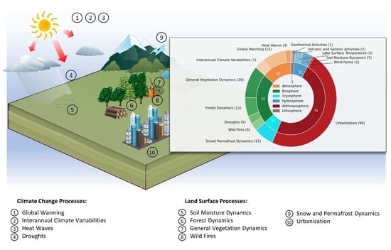
3.3. Research Topics

In the following section, the research topics that were identified from the reviewed articles are described. One or more topics were assigned to each study, and the studies were then sorted into six spheres based on their thematic foci: “Atmosphere”, “Biosphere”, “Cryosphere”, “Hydrosphere”, “Anthroposphere” and “Lithosphere” (Figure 6). More than half of the studies (91, 55.4%) were focused on the Anthroposphere, of which 90 were conducted in the context of Urbanization and SUHI, respectively. The second-most represented sphere is the Biosphere (42, 25.6%), where most studies linked general vegetation dynamics with LST dynamics, followed by forest dynamics, droughts and wildfires. Fewer studies focused on research topics assigned to ‘Atmosphere’ (26, 15.8%), ‘Cryosphere’ (13, 7.9%) and Hydrosphere (12, 7.3%). Only three studies were categorized into ‘Lithosphere’. It should be mentioned that several studies dealt with multiple topics, which can even be assigned to different spheres; for example, studies dealing with general vegetation dynamics also dealt with soil moisture dynamics [26,29], snow-and-permafrost dynamics [29], droughts [24,25], urbanization [51], heat waves [20] and global warming [15]. The next Section 3.3.1, Section 3.3.2, Section 3.3.3, Section 3.3.4, Section 3.3.5 and Section 3.3.6 provide an overview of the topics and summarize the links between LST dynamics and global change in each sphere.

3.3.1. Anthroposphere

The most drastic land cover change can be attributed to urbanization, where impervious surfaces replace natural surfaces, e.g., evaporative vegetation and water area. This transition has a significant impact on the urban climate, resulting in a temperature gradient between the urban area and its surroundings from the surface to the canopy level, which is called the urban heat island (UHI) effect. The only way to measure and quantify the UHI with remote sensing data is through the Surface Urban Heat Island (SUHI) effect, which is the difference between the LST over urban areas relative to neighboring non-urban areas [2]. In most cases, this difference is positive, which was also reflected in our reviewed studies [64,66,67,81,82,83,85,93,98,102,110,124,128,129,133,137]. However, in arid climates, where the non-urban environment is not covered by vegetation, it can also be negative [75,76,132,139], which is referred to as an urban heat sink.

The intensity and spatio-temporal form of the SUHI vary from city to city. Several factors have been described in the literature, such as the ratio of impervious surfaces to vegetation or water surface within the city, which is the most determining factor of the SUHI [2,90,103,139,160]. Some of the reviewed studies emphasize the role of parks, forests and lakes as a cooling factor for the cities affected by the SUHI [64,74,79,81,94,97,100,102,105,106,110,123,125,129,131,138,141]. On the other hand, an increase in SUHI intensity and hot day frequency can be directly attributed to increased urban density [89,133,142,143,167,168]. A second factor is the urban landscape, where high buildings and trees can have a shading effect on the thermal environment [74,102,110,112,122]. Further factors are the reflective properties of the materials used in the urban environment [88,100,112], climate [65,85,118,121,135,140], the size of the city [96,142] and human activities, such as heating in winter [126,135]. Additionally, the SUHI intensity and footprint underlies diurnal and seasonal variations [100], with higher intensity during summer [143,169] and daytime [114,135].

The UHI effect can intensify the impact of heat waves on human health and is, therefore, a key topic in the domain of climate change research. Furthermore, the LST can be used to quantify the heat stress inside urban areas, which is expected to be more severe in the future due to global warming [2,160]. Wei et al. [133] reported an increase in hot day frequency between 0.59% and 7.17% in global megacities between 2003 and 2020. For the heat wave in June 2018, extreme LSTs were reported over Los Angeles county [95]. During the heat wave in North America in 2021, the LSTs over several cities reached a record level; however, the intensity of the SUHIs did not increase [85].

The global, continental or regional impact of SUHI on LST dynamics is hard to quantify because the measured dynamics and intensity of the SUHI strongly depend on the definition of the urban and nonurban reference and the time of observation. On the city scale, the intensities of SUHI mostly range between 0 and 5 K [73,80,83,98,126,128,135,168,169], but when comparing the LSTs of impervious surface areas or densely built-up core cities directly to vegetated areas on extremely hot days, the differences can reach up to 7–15 K [72,73,125,142]. Regarding SUHI dynamics, it becomes clear that the LST inside urban areas is increasing at a higher rate than outside the cities, leading to an increase in the SUHI effect in the order of 0.4–0.7 K/decade [92,104,117]. The study by Zhao et al. [145] for Zhengzhou City showed a warming rate in terms of LST of 2.72 K in the last three decades, which exceeds the global LST increase in the magnitude of 0.03 K/year [170]. Regional studies in Hainan, China [68], over the Central Himalaya [16], and in West Bengal, India [51], showed a direct link between urbanization and the regional increase in LST. Ding et al. [71] proposed a phenology shift of nine days earlier in spring and six days later in autumn, triggered by rapid urbanization and subsequent LST increase. Therefore, urbanization can be seen as one of the main drivers of LST increase, exceeding the local scale.

Chang et al. [171] analyzed the effects of wind farms on LST, concluding that wind farms have a warming effect on nighttime LST, which is, however, weaker than the SUHI effect.

3.3.2. Biosphere

The difference in the thermal properties of vegetated surfaces in comparison to barren areas can be attributed to three factors: first, vegetation usually has a lower albedo than areas covered with soil, stone or sand, meaning that a bigger portion of the incoming shortwave radiation from the sun is transformed, heating the surface. The second factor relates to the complexity of the surface vegetation, leading to an increase in thermal inertia. The third factor is the increase in evaporative cooling over vegetated areas, which is a consequence of the active water cycle of plants.

In warm months, during the daytime, evaporative cooling is the dominant factor, leading to a general cooling effect in terms of vegetation. This can be verified through the negative correlation between different vegetation indices and LST; the negative relationship between NDVI, EVI and LST was analyzed globally by [34]. Over North America, NDVI and LST showed a strong negative correlation for the months from May to October [24]. Regional and local studies showed a negative relationship between NDVI, LAI and LST in the USA [42], between NDVI and LST in Cyprus [45] and in India [51] and between the Enhanced Vegetation Index (EVI) and LST in Vietnam [25]. Nill et al. [29] showed a cooling of summer LST in the Arctic Mackenzie Delta Region (Canada), which was well correlated with the large-scale wetting and green-up in this region. Sun et al. [24] state that the cooling effect of vegetation during the daytime is much stronger than during the nighttime.

During winter and spring, the relationship between NDVI and LST can be positive because of the thermal inertia of the vegetation acting as temperature storage. A positive correlation between NDVI and LST was, e.g., found throughout all European biomes by [47] during the springtime (March–May), and also over North America during winter [24]. According to Karnieli et al. [47], the direction of the relationship between NDVI and LST can be an indicator if energy (when the relationship is positive) or water (when the relationship is negative) is a growth-limiting factor. Therefore, with the cooling effect on a warm background climate and the warming effect on a cool background climate, vegetation can be seen as a regulating factor of LST [172].

While the vegetation state shows a clear influence on the LST, LST itself, in turn, is an important indicator to derive phenology parameters. One example is the derivation of growing degree days (GDDs), which is the sum of days with a higher mean temperature than 10 °C during the growing season [49]. LST-derived GDDs can be used to monitor shifts in phenology, as carried out in [41] over South Korea.

The regulating effect of vegetation on LST is especially high in forests, which usually have a higher surface roughness and evapotranspiration than open land. Generally speaking, afforestation can increase the LST north of 45°N and reduce the LST south of 35°N in the northern hemisphere [31]. Deforestation, on the other hand, had a warming effect on the average trends, with an additional 0.28 K per decade in tropical regions and a cooling effect on the average trends, with −0.55 K in boreal regions [37]. The impact of deforestation on global warming is particularly noticeable in tropical regions, where the wide tropical forests are threatened by agricultural and urbanization processes. The decrease in evapotranspiration and surface roughness, which are associated with LST warming, mostly dominate the cooling effect of the increase in albedo. In East Africa, deforestation caused a net warming effect on LST of 1.3 K between 2001 and 2013 [35]. In the Amazonas region, LST increases due to deforestation have been reported from Xinga, Brazil [38], and Caatinga, Brazil [36]. In South East Asia, increased LST could be measured up to 6 km away from the forest disturbance site [33]. In Brazil, increases in maximum LST due to forest loss were noticed even within a 50 km distance [32].

In the temperate climate zone, the relationship between forest cover and LST is more ambiguous. For Europe, forests have a cooling effect on the daytime during warm seasons and a warming effect on the day and nighttime during cold seasons. The cooling effect dominates the warming effect, resulting in a net cooling effect across Europe, except for the northeastern part. Tang et al. [31] also emphasize the importance of forests for temperature regulation during heat waves. Their results suggested that above the background temperature of 6.5 °C, forests have a cooling effect on LSTs. For Guangdong, China, it was shown that forest gain has the potential to reverse the effects of forest loss on LST [30].

In boreal regions, wildfires are a bigger threat to the forest than anthropogenic activities. Fires transform forested or other vegetated areas into bare land and lead to an increase in LSTs on the one hand and to an increase in LST seasonal and diurnal amplitude on the other hand [28,52,53,54,55]. In return, the rise in LST increases the probability of fires, building a self-reinforcing process [53]. In Siberia, Liu et al. [28] showed a net warming effect of 0.325 K one year after a fire in an evergreen needleleaf forest, resulting from strong summer warming and weak winter cooling in the affected areas. For deciduous forests, the net warming was much lower (0.0728 K) because of a much weaker warming effect in summer. While the warming effect in summer can be attributed to a decrease in evapotranspiration, the cooling effect in winter is dominated by the increase in albedo, also partly because open land tends to be more often covered with snow than forest.

Droughts are characterized by abnormal vegetation and surface moisture states and have a huge impact on the LST. During droughts, the precipitation shortage leads to a reduction in soil moisture and, as a consequence, to a reduction in vegetation water availability. Once the soil dries out, the evaporation process stops and LST increases. Additionally, plants close their stomata to reduce water loss through transpiration, and this closure leads to a rise in canopy temperature [22]. Therefore, LST is a key parameter to assess the spatio-temporal extent and the severity of droughts. Several indices exist that use LST and vegetation parameters to describe water stress, e.g., the Temperature Condition Index [173], the Vegetation Temperature Condition Index [174], and the Normalized Difference Temperature Index. A detailed description of these indices is out of the scope of this review and it is provided by AghaKouchak et al. [164]. Droughts usually result in an increase in LST; for example, over the Mekong River Delta [25]. Forests can buffer this effect because trees have access to deep soil water and can, therefore, maintain transpiration [21].

3.3.3. Atmosphere

In addition to land cover changes, which lead to LST changes within a short time, long-term trends of LST can provide deep insights concerning the climate change of our planet. While the difference between instantaneous LST and air temperature can be high, there is a strong agreement in long-term trends between these two variables [155,175]. This, and the fact that thermal remote sensing data have been around for decades now, make LST a valuable resource for measuring global warming. Sobrino et al. [4] analyzed the global surface temperature between 2003 and 2016, concluding that there is a positive global LST trend of 0.03 K/year, which is more than twice as high as the global SST trend (0.013 K/year). Especially strong LST warming can be observed in the Northern latitudes [4,15]. Further hotspots are the USA, northern Brazil and Patagonia [4]. Negative LST trends can be observed over Arabia, India, China, Australia and Antarctica [4,15]. The LST cooling over Antarctica can possibly be attributed to the Ozone hole [15]. NourEldeen et al. [12] analyzed LST trends over Africa between 2003 and 2017 and observed significant warming trends in the winter season, May and September. Abera et al. [35] equally observed positive and negative LST trends over East Africa during the daytime and consistent positive trends during the nighttime. In general, nighttime LST trends are lower but more consistent than the daytime trends [3,5,12,13,16]. Furthermore, they are more consistent with the air temperature because LST and air temperature decouple at higher temperatures [176]. Therefore, global warming is more pronounced at nighttime LST trends than during the day [3]. In addition to global warming, interannual climate variabilities, such as the El-Nino-Southern Oscillation (ENSO), the North Atlantic Oscillation (NAO), the Pacific Decadal Oscillation (PDO) or the Pacific North American Pattern (PNA), are reflected in the LST time series. Abbas et al. [6] observed a significant influence of NAO, ENSO and PDO on anomalies of mean LST over the Tarim Basin in Northwest China. Over Alberta, Canada, the PNA had the greatest influence on LST; however, none of the relationships between atmospheric oscillations and LST warming were significant [9].

Similar to droughts, heat waves are extreme climatic events that have severe impacts on a wide range of societal and environmental domains. They are linked to increased mortality rates, stress on animal populations and ecosystems and a higher probability of energy infrastructure failures [19]. The occurrence of heat waves has increased in recent decades due to climate change. Examples are the European heat wave in 2003 [177], the Russian heat wave in 2010 [178] and the heat wave in Western North America in 2021 [179]. Despite there being no clear definition of heat waves, most studies consider heat waves as a consecutive number of days where temperatures are hotter than the climatological mean of this period. Heat wave metrics, therefore, are mostly based on positive LST or air temperature anomalies in the warm season. Agathangelidis et al. [19] showed that, for the Mediterranean region, there is a high coincidence rate between heat wave days, detected with air temperature station measurements and LST anomalies. The match percentage was lower on the first days of the heat wave and increased as the heat wave evolved. During the study period between 2002 and 2020, they noticed an increase in positive LST anomalies of 1.35 days/10 years during the daytime and 1.64 days/10 years during the nighttime, which was in line with the increase in heat wave days. Major events, such as the European heat wave in 2003, could be clearly detected from the number of LST anomaly days [19]. The global analysis of yearly maximum LST by Mildrexler et al. [180] showed spatially continuous patches of positive LST anomalies over Europe in 2003 and Siberia in 2010, which corresponds to the reported heat waves. Albright et al. [18] analyzed the impact of heat waves on the avian community in the central USA using MODIS LST and Ta measurements. They concluded that heat wave models based on LST provide more ecologically relevant information because they are an indicator of both temperature and vegetation conditions.

3.3.4. Cryosphere

In the cold regions of the world with high latitudes and high elevations, climate change becomes particularly visible through the melting of glaciers, permafrost degradation and changes in the snow season. All of these processes lead to rapid changes in LSTs, for which reason high LST dynamics can be found in these regions. The global evaluation of MODIS LST between 2003 and 2016 showed that the LST trend for the high latitudes of the Northern Hemisphere was almost twice as high as the global trend [4]. Higher warming rates for higher elevations have been found in many mountain regions [165]. Zhao et al. [16] reported increasing warming rates with higher elevations for the central Himalayan region. Pepin et al. [61] and Ran et al. [62] found that warming rates peak at around 5000 m, which corresponds with the elevation of the snow line retreat. However, Choudhury et al. [59] report decreasing LST trends for the Northwest Himalaya region, which correspond with the increase in snow cover area in this area.

LST is a direct indicator of the distribution of permafrost. Langer et al. [58] showed that the LST time series over the Lena Delta in Siberia is suitable for modeling the evolution of the Permafrost state when the snow conditions are correctly estimated. The degradation of permafrost was analyzed in North East China [63] and the source region of the Yellow river on the Tibetan Plateau [57] with the ground surface freezing index (DDF), which is the number of days with LSTs below 0 °C. Batbaatar et al. [56] mapped the permafrost with the ‘zero curtain’ phenomenon, which describes the freezing and thawing phase of the ground in spring and autumn, where LST remains around 0 °C.

3.3.5. Hydrosphere

In addition to albedo and surface roughness, the water content of the surface is a critical parameter that determines its thermal behavior. Water changes the energy balance of the land surface and increases its thermal inertia. This reduces the diurnal as well as the annual amplitude of LST [161]. LST is a key indicator of soil moisture status and, therefore, widely used to detect water stress and droughts [22]. For that, either LST inertia is used, which can be obtained from multiple LST measurements per day (e.g., at sunrise and sunset), or the normalized difference temperature index (NDTI) is computed, which relates the actual LST to hypothetical LST values in extreme wet and dry states. These extreme LSTs can be obtained from the energy balance principle [161]. Over vegetated areas, the canopy temperature can be an indicator for soil moisture because an increase in canopy temperature indicates less evapotranspiration, therefore, water stress and decreased soil moisture. This connection is expressed through the Crop Water Stress Index [161]. A European-wide study by Cammalleri et al. [22] showed that LST anomalies are a good proxy for the soil moisture status. A local study over the Duero river basin in Spain showed a strong negative correlation between maximum LST and soil moisture in summer, autumn and spring, while in winter, there is a decoupling between soil moisture and LST [23].

In addition to droughts, declining wetlands, driven by climate change and anthropogenic transformation of land cover, have a noticeable impact on global LST dynamics. Wu et al. [27] stated that, in tropical regions, wetlands have a cooling effect, while in boreal regions, wetlands have a warming effect. The expansion of rice fields in the Sanjiang Plain in northeastern China, on the other hand, showed a significant cooling effect on LST for this region [26].

Another topic related to the LST is the lake surface water temperature (LSWT). Changes in LSWT are a valuable resource for tracking climate change. On the other hand, they can alter a lake’s biological productivity and greenhouse gas emissions [181]. The assessment of LSWT in Nevada and California showed that the change rates are an order of magnitude higher than the global SST trend and about as twice as high as the regional air temperature trend [14]. Mostly decreasing LSWT trends were found over the Tibetan Plateau [182] and the North American Great Lakes [183].

3.3.6. Lithosphere

While the previously discussed topics are well-established applications of LST, only a few studies can be found using LST to describe processes in the Lithosphere. Furthermore, these studies seem to have more of an experimental character. The relationship between LST and volcanic activity was analyzed by Caputo et al. [184], while Blackett et al. [185] explored LST as a predictor of earthquakes. However, both studies found no evidence that these processes are connected to LST dynamics. Nevertheless, Silvestri et al. [186] successfully detected geothermally active areas with Landsat LST.

3.4. Employed Sensors

Figure 7a displays the number of studies per sensor system or sensor system combination. The most commonly used sensor system in our reviewed studies was the MODIS, with 86 (52%) studies using it, using MODIS as a single data source, and an additional 12 (7%), which used MODIS in combination with other sensors. This is in line with the results of Phan & Kappas [166], which not only identified MODIS as the most common thermal sensor but also observed a steady increase in publications related to MODIS LST between 2009 and 2018. The MODIS is onboard the satellites Terra and Aqua, which were launched in 1999 and 2002. With both satellites, MODIS provides a very high temporal resolution (four times a day) combined with a medium spatial resolution (1 km in the thermal channels) for quite a long period (>20 years), which makes it popular for time series studies from the regional to the global scale. Another reason for its popularity is its wide range of freely available quality checked and validated products, which are not only limited to thermal products.

After MODIS, the sensors from the Landsat family are the second-most commonly used in our reviewed studies, with 55 (34%) studies using Landsat as a single data source and an additional 11 studies (7%) using Landsat in combination with other sensors. The Landsat mission comprises eight successful generations of satellites (Landsat 1–9; Landsat 6 failed), of which five generations (from Landsat 4) carried thermal sensors. Landsat 4–5 carried the Thematic Mapper (TM), Landsat 7, the Thematic Mapper Plus (ETM+), and Landsat 8 and 9, the Thermal Infrared Sensor (TIRS). The spatial resolutions of the thermal Landsat data are relatively high, with 120 m (TM), 60 m (ETM+) and 100 m (TIRS); however, the temporal resolution is quite low, with a revisit time of 16 days. The Landsat mission has provided thermal remote sensing data since 1982, which is the longest time series of this kind besides AVHRR. Since 2008, the Landsat archive has been freely accessible to scientists [2].

Rarely, other sensors were used. We counted three studies each for ASTER and ECOSTRESS, two studies each for GOES, ATSR and AVHRR and one study for AATSR counting in the studies, which used these sensors in combination with other sensors. Mounted on a geostationary satellite, GOES provides a high temporal (3 h) but a low spatial resolution (4 km). Similar to MODIS, ASTER is mounted on the Terra satellite and combines a similar high spatial resolution as Landsat (90 m) with the high temporal resolution of MODIS (twice daily). However, until 2016, ASTER data were chargeable, which prohibited their wider use [2]. The ATSR on the ERS-1 and 2 satellites and its successor, AATSR on ENVISAT, only provide a low temporal resolution (35 days), wherefore their thermal data are mostly used for SST. ECOSTRESS is a relatively new sensor (in orbit since 2018) and therefore provides only a short time series. The AVHRR on the NOAA satellites combines the high temporal resolution of MODIS with a long time series (the first LST products have existed since 1981), providing a valuable data source to quantify long-term processes, such as climate change. However, the 16 generations of satellites have different overpass times and experience orbits, meaning that it is difficult to create a harmonized LST time series [157,187,188,189]. Fifteen of the reviewed studies (9%) used a combination of sensors, whereby more than half of them used the combination of MODIS and Landsat. This combination can supplement the high temporal resolution of MODIS with the high spatial resolution and the long time series of Landsat; however, upscaling or downscaling methods are necessary to integrate the different spatial resolutions.

Figure 7b shows the number of studies per sensor system in each research sphere. For all research spheres but Anthroposphere, MODIS LST is by far the most commonly used data source. The increased use of Landsat LST in the context of SUHI and Urbanization can be explained by the high spatial variability of the urban landscape, which necessitates the high spatial resolution of Landsat. Furthermore, in many studies in this research field, the focus is more on the quantification of the LST difference between the urban and non-urban areas than on temporal dynamics. In these cases, a high spatial resolution outweighs frequent measurements, and observations are often multitemporal at intervals of several years. Examples of this are the studies by [117,123,124,130,167]. The reviewed studies, which used Landsat data in a non-urban context, were mostly on the local scale, benefiting from Landsat’s high spatial resolution.

3.5. Spatial Scale and Resolution of Reviewed Studies

Figure 8a shows an overview of the spatial resolutions in our reviewed articles. The distribution of the spatial resolution reflects the employed sensors of the corresponding studies. Nearly half of the studies (77, 47%) were conducted with a medium resolution, which is the original resolution of MODIS LST. Only two of these studies did not use MODIS LST, namely Ouyang et al. [190], who used AATSR LST to analyze local LST trends over the Heihe River Basin in China, and Hrisko et al. [65], who used GOES LST to analyze LST trends over major US cities. After medium resolution, the second-most reviewed studies (57, 35%) used high-resolution LST, which comprises the original resolution of Landsat, ASTER and ECOSTRESS. Fifty of these studies used Landsat LST, while two studies used ECOSTRESS, one study used ASTER, and another two studies used a combination of ASTER and ECOSTRESS. Forty-eight (81%) of the studies, which used high-resolution LST, were in the context of SUHI. The remaining studies were conducted in the context of heat waves [20], general vegetation dynamics [20,29,49,51], wildfires [54], permafrost [29], lake surface temperature [191], soil moisture dynamics [29], volcanic and seismic [184] and geothermal activities [186]. Twelve studies (7%) used a medium–high resolution, which mostly results from a fusion of multiple data sources, e.g., MODIS and Landsat [85,102] or different Landsat generations [104]. Sixteen (9%) of the reviewed studies used a medium–low resolution, of which 11 studies [4,5,8,9,10,12,15,18,28,34,37] used the MODIS LST composites from the MOD11C*/MYD11C* product suite. These products are especially convenient for global- or large-scale studies because they provide global coverage on a 0.05° grid. Equally, the studies that used a low spatial resolution were conducted on global [10,140], continental [24], or large regional [3,42] scales.

Concerning the spatial scale, almost half of the studies (79, 49%) were conducted on a local scale (Figure 8b). Fifty-five of the local studies were concerned with SUHI, whereby these studies mostly analyzed the SUHI of one certain city. Nine local studies were found in the context of general vegetation dynamics, which were case studies analyzing the interaction between vegetation and LST over a small region. Out of the five studies dealing with wildfires, four were also conducted on a local scale. The second most analyzed scale is the ‘regional large’ scale, with 38 (23%) studies. The studies from this category were mostly conducted on a national scale for large countries (USA, China, India) or were multi-national. While again, the most studied topic in this category is SUHI (17 studies), topics from the sphere of ‘Atmosphere’ were overrepresented (eight studies). These studies include the examination of the Mediterranean and North American heatwaves [18,19] and climatological long-term trends over east Africa [3] and the Tibetan Plateau [61]. The third most-studied spatial scale is regional small‘ (21 studies, 13%). These studies mostly analyzed LST dynamics for smaller countries (e.g., Nepal, Vietnam, South Korea) or limited regions within, e.g., China. Again, almost half of the studies (10) in this category were in the context of SUHI. The second-most addressed research sphere in this category is the ‘Biosphere’ (six studies), including the assessment of spring phenology changes in South Korea [41], the analysis of drought dynamics in the Mekong River Delta [25] and the analysis of deforestation effects in Southern Amazonia [38]. Only 14 studies (9%) were conducted on a global scale, and even fewer (nine studies, 6%) were conducted on a continental scale. Within the continental studies, the most studied continent by far is Europe (six studies). These studies cover different topics, e.g., Tang et al. [31] studied the effects of forests on LST, while Cammallieri et al. [22] analyzed the relationship between LST and the soil moisture status and Hellings & Rienmow [66] mapped the LST dynamics of urban areas. Further, continental studies investigated the NDVI-LST relationship in North America [24], the SUHI effect across South America [135] or long-term trends of LST over Africa [12]. On the global scale, studies investigating the relationship between vegetation and LST [15,34,37,40] and studies in the context of global warming [4,5,15] dominate. However, there are also four global studies in the context of SUHI [118,121,133,139] and one study investigating the global effect of wetlands and LST [27]. Almost no global or continental study employed a high or medium–high spatial resolution.

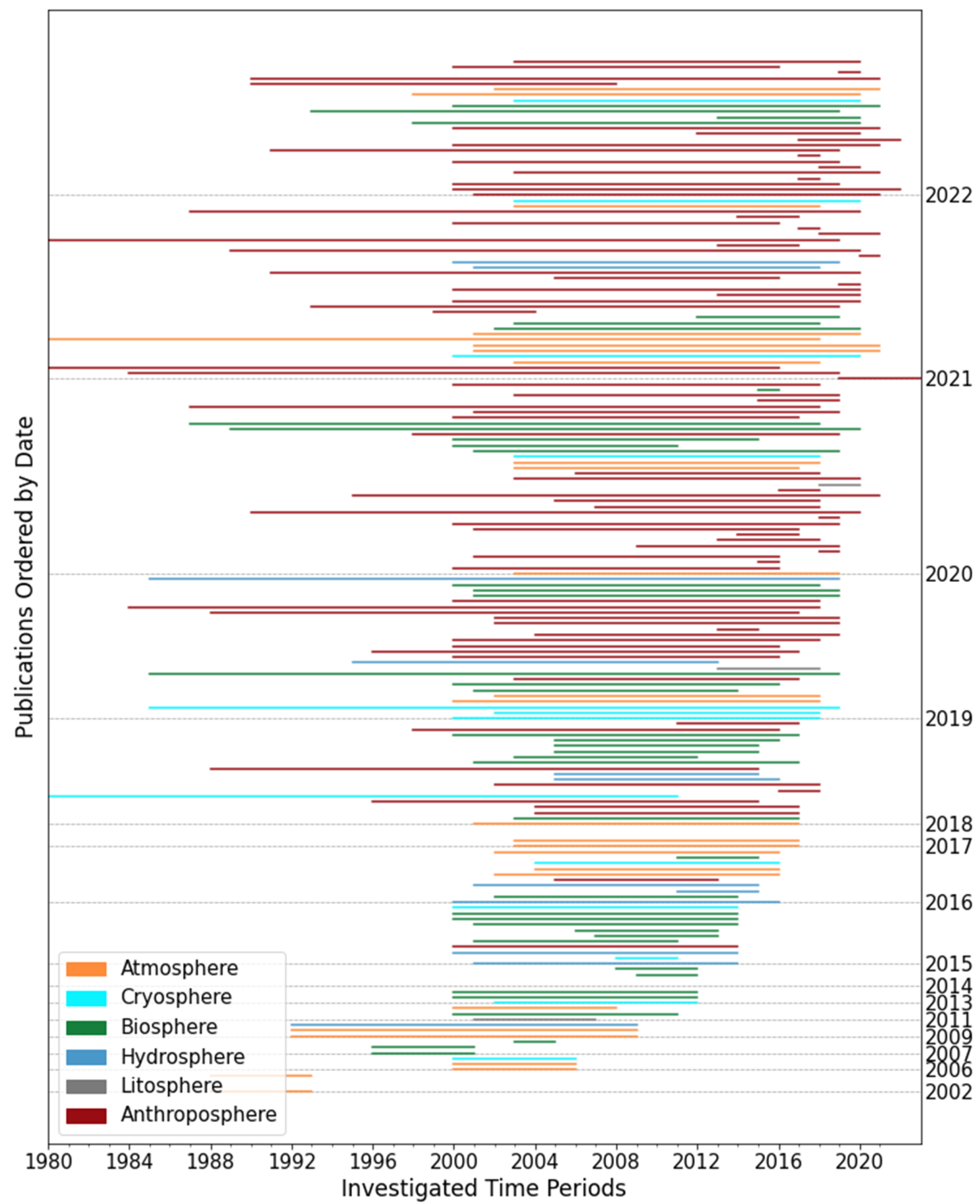
3.6. Temporal Scale and Resolution of Reviewed Studies

Figure 9a shows the distribution of the temporal resolutions of our reviewed studies. The majority of the studies (108, 67%) analyzed an LST time series, probably owing to the dedicated focus of this review on LST dynamics. However, not a small part of the reviewed studies (45, 28%) were conducted with multitemporal time steps, whereas only a few studies used bitemporal (four, 2%) or monotemporal (five, 3%) resolution. The monotemporal, as well as the bitemporal studies, were exclusively conducted in the context of SUHI. Four of the monotemporal studies analyzed the influence of urban features (building height and proximity of vegetation and buildings [74], the presence of green spaces [131,138] and construction sites [128]) on LST, while one monotemporal study examined the relationship between long-term mean urban LST and long-term mean precipitation [140]. The bitemporal studies are concerned with urban green spaces [106], the SUHI effect in desert megacities [107], the effects of land use on SUHI [94] and the assessment of urban renewal processes [113]. For the multitemporal category, the SUHI studies dominate, making up 34 of the 45 studies. However, here we also found some studies with other research topics, e.g., in the context of heat waves [20], forest dynamics [30,36], general vegetation dynamics [42,48,51], wildfires [54,55] and LSWT [191].

While in the mono-, bi- and multitemporal categories, most studies use Landsat LST, in the time series category, MODIS is the most common sensor. Figure 9b depicts the distribution of the time series frequencies in the 108 studies that employ an LST time series. The most common frequencies are daily (26 studies, 24%), weekly (28 studies, 26%) and monthly (27 studies, 25%), which are at the same time as the temporal resolutions of the freely available MODIS LST composites products MOD/MYD11C1, 2 and 3. Nineteen studies used either a quarterly, annual or multiannual temporal resolution. Most of these studies either employed a long time series [46,91,119] or conducted their study on a global or large spatial scale [4,15,28,33,93]. The low temporal resolution here was probably employed to keep the amount of data computational.

Figure 9c shows the distribution of the time series length for all studies that employ an LST time series. The time series length ranges from under a year to 57 years. The median length is 14 years. Looking at the study periods in Figure 10, the majority of the time series studies start around the year 2000, which corresponds with the launch dates of the Terra (1999) and Aqua (2002) satellites carrying the MODIS sensor. Despite the time series length tending to increase with the publication date, most of the study periods are shorter than 25 years. To be exact, 54% of the time series studies had a study period shorter than 15 years, 88% had a period shorter than 20 years, and 93% had a period shorter than 30 years. The studies with a time series longer than 25 years either used Landsat LST [29,45,46,91,119,192] or extended their MODIS time series with air temperature records [62] or simulated LSTs from meteorological data [17].

Figure 11 also displays the study periods of the time series studies but with this time categorized by their covered research spheres. Two things become visible: First, observing the y-axis, the research spheres are quite evenly distributed, and there is no trend noticeable concerning a certain research sphere. The few long-term time series studies were not limited to one research sphere but were conducted in almost all different research spheres except the lithosphere.

3.7. Methods Used for the Analysis of LST Dynamics

The following section provides an overview of the most important methods for the analysis of LST dynamics from our reviewed studies. For our analysis, the methods have been sorted into the categories of spatial LST analysis and temporal LST analysis. The methods for the spatial analysis have been further classified into methods concerned with spatial anomalies and the spatial regression between LST and other variables. The methods for the temporal analysis have been further classified into methods for the preparation of the LST time series, the analysis of linear temporal trends, the analysis of temporal anomalies and the analysis of the temporal regression between LST and other variables. Several studies employed methods for spatial and temporal analysis, e.g., first quantifying the magnitude of SUHIs, and in the second step, observing their temporal trends.

3.7.1. Spatial LST Analysis

Analysis of Spatial Anomalies: Usually, LST values follow the order of Gaussian or T-distribution in the spatial as well as the temporal dimension [1]. To be defined as a spatial anomaly, a spatially connected pattern of LST must fulfill two criteria: First, it must deviate from the spatial average of neighboring pixels (reference area) within a defined area to a certain degree. Second, it should have a certain spread to distinguish it from an outlier [1]. A typical example of a spatial anomaly is the SUHI. The most straightforward way to quantify a spatial anomaly is to relate the LST within the spatial anomaly to the LST of the reference area, e.g., by subtracting the mean LST of the rural reference from the mean LST of the urban area [118]. However, in this case, the definition of the urban and the rural reference area is crucial [88,119,146]. An alternative to employing fixed urban extents is the statistical derivation of the urban area by analyzing the decay of LST from the urban center and then automatically calculating a threshold to delineate the urban area [114]. Related methods are the Gaussian surface model and the kernel convolution method [2].

Spatial Regression between LST and other Variables: Several studies analyzed the relationship between LST and other variables by regressing observations of LST with observations of these variables from the same location and time. The regression analysis allows assumptions about how a certain variable is influencing LST, e.g., from the negative relationship between NDVI and LST [42], the cooling effect of vegetation can be derived. The correlation between LST and the respective variable is often described by the correlation coefficient (R) or the coefficient of determination (R²), which are measures of the strength of the correlation and a linear equation describing the direction of the relationship. To analyze the relationship between multiple variables (e.g., LST, ET and albedo), a multiple regression model can be applied [35]. In addition to classic statistical methods, machine learning techniques have also been employed to analyze influencing factors on LST, e.g., the Random Forest model [6].

3.7.2. Temporal LST Analysis

LST Time Series Preparation: Because of the significant influence of solar radiation on LST, LST time series mostly have a seasonal signal. To derive time series statistics as anomalies or the linear trend one must account for this seasonal signal. One method is to decompose the time series into its components of seasonality, randomness and trend, which is the additive seasonal decomposition by moving average. This method was applied by [45] to monthly Landsat LST. Another method to account for seasonality is the derivation of annual statistics by employing an annual temperature cycle model, which is usually described by three or five parameters [1]. A three-parameter model was applied by [16]. A further possibility to deal with the problem of seasonality is the calculation of monthly climatologies, e.g., carried out by [35]. Another common problem is missing LSTs due to cloud contamination. Missing LSTs can be either interpolated from temporal neighboring pixels [34] or spatial neighboring pixels [12]. However, already in the introduction, the clear sky bias was mentioned, referring to the problem that remotely sensed LST derived under clear sky conditions is not representative of all-weather conditions. None of the reviewed studies employed respective LST correction terms to account for the difference between clear-sky LST and LST under clouds [154].

Analysis of Linear Temporal Trends: One of the most analyzed properties of an LST time series is the linear temporal trend. The linear trend in LST indicates the uniform change in LST within a certain time period and, therefore, also allows for the prediction of LST dynamics in the future. Two different methods are used to measure the linear trend: The most straight-forward method is the ordinary least square regression between LST and time. The ordinary least square regression minimizes the sum of squared residuals for the linear model. The advantage of this method is its simplicity. However, it is quite sensible to outliers. A more robust method is the Theil–Sen Estimator, which first computes the slopes of all lines through pairs of points and then calculates the median of these slopes. The Theil–Sen Estimator is often used together with the Mann–Kendall Test, which determines if a trend is significant regarding a certain significance level indicated by the p-value. This is important to translate the statistical trend, which also could be a random result, into meaningful statements. The lower the p-value, the higher the significance level. In our reviewed studies, the p-values were either set to 0.1 (low significance) [34], 0.05 (medium significance) [6,12,16] or 0.01 (high significance) [5]. Linear temporal trends of LST have been analyzed for various regions and on various scales; for example, least square regression has been used to derive global land surface temperature trends in the context of global warming and vegetation dynamics by [15,170]. The Theil–Sen Estimator, together with the Mann–Kendall Test, has been used to derive LST trends over Africa [12], the Himalaya [16] and Northwest China [6], over global deserts [5] and globally [4,34].

Analysis of Temporal Anomalies: Analogous to the spatial anomaly, a segment of an LST time series must fulfill two criteria to be defined as a temporal anomaly: First, it must deviate from the moving average of the time series to a certain degree, which is usually determined by the variance of the LST values around this moving average. Second, it should last for a range of time to not be considered an outlier [1]. Typical applications of positive LST anomalies are the quantification of heat waves and droughts: Albright et al. [18] derived several heat wave metrics from positive LST anomalies, while Agathangelidis et al. [19] correlated heat wave days measured with air temperature with positive LST anomalies. Cammallieri et al. [22] found that LST anomalies are a good proxy for soil moisture status and, therefore, a valuable indicator for droughts. Muster et al. [60] used temporal LST anomalies to detect changes from vegetated to barren land over Northern Canada.

Temporal Regression between LST and other Variables: In addition to regression between LST and other variables at the same location and time (spatial regression), the time series between LST and other variables can be compared; for example, LST dynamics have been analyzed with respect to vegetation indices [15,34,39,193], albedo and heat fluxes [3] and atmospheric oscillations [6,17]. Common time series features can be observed visually on the one hand [6] and quantified by statistical measures on the other hand. To link the time series of LST to the time series of one or multiple other variables, either observations for the same period can be correlated or time series models can be applied, and the resulting models can be compared afterward. Song et al. [15] used Pearson’s correlation coefficient to correlate LST observations and NDVI observations from the same year. If there is an expected time lag between the determining and the responding variable, e.g., for the response of LST to drought indices [45], this can be analyzed via cross-correlation, which correlates observations of LST with the drought indices of previous months. Amantai et al. [17] applied wavelet functions to the time series of LST, wind speed and relative humidity before comparison to overcome different time scales and frequency ranges. Andronis et al. [45] used the BFAST model to cross-check abrupt changes in the trend lines of LST and NDVI. If the effect of one special variable on LST should be isolated, it is sometimes necessary to control the effects of other continuous variables. This was performed using covariance analysis by Caioni et al. [21] and partial correlation by Song et al. [15]. Abera et al. [35] subtracted a climate background signal from LST change to isolate deforestation effects on LST. [33,119] compared LST trends for pixels affected and unaffected by deforestation for the same problem.

4. Discussion

4.1. The Need for LST Time Series Studies in the Context of Global Change

After filtering our WoS search terms, English language, open access and WoS categories, our search returned 1095 results (Figure 3). However, only the minority of these results (203 studies) eventually fit the scope of our review by analyzing LST dynamics in the context of global change. The majority of the LST-related studies we have found were either concerned with the validation of LST retrieval methods, the validation of LST fusion and reconstruction models or the validation of air temperature derivation from LST. While validation studies are necessary, especially from the point of view of climate-change-related studies, which require a high accuracy and stability of LST [148], the use of existing remote sensing LST datasets to study global change processes should be extended. Although the majority of our reviewed studies employed an LST time series, a significant number of studies analyzed mono-, bi- or multitemporal LST measurements (Figure 9a). While these snapshots can reveal spatial patterns, e.g., the magnitude of SUHI, they are often not representative of the diurnal and seasonal variations of LST. High temporal resolution time series are therefore recommended to analyze this in the temporal dimension’s highly fluctuating variables.

4.2. Dominance of the MODIS Sensors for LST

The investigation of the sensor systems, which were employed in the reviewed studies, showed that MODIS is by far the most popular sensor system for the investigation of LST dynamics. The reasons for its popularity are its high temporal resolution, its constant revisit times and the wide range of freely available, quality-checked and well-validated products. However, the National Aeronautics and Space Administration (NASA) announced that MODIS will be decommissioned in the upcoming years. The designated successor of MODIS is the VIIRS sensor which has been in orbit on NASA’s Suomi NPP satellite since 2011 and on the NOAA 20 satellite since 2017. However, our results suggest that VIIRS LST is not yet used in the LST research community. This will probably change after the decommission of MODIS. Because the Terra and Aqua satellites carrying the MODIS sensor were launched in 1999 and 2002, the MODIS LST time series today is limited to 22 years. However, study periods should be ideally longer than 30 years to make climate-relevant statements [187].

One sensor, with a similar temporal and spatial resolution as MODIS but longer operation time (from the early 1980s), is AVHRR. Because of its similarities to MODIS in terms of acquisition conditions, it is a candidate for the extension of the MODIS LST time series. However, the AVHRR has been mounted on 15 different satellites with different observation times. Furthermore, a number of these satellites are experiencing orbit drift, meaning that during their lifetime their equator-crossing times shift from noon toward the evening. The effects of daytime shifts and orbit drift on AVHRR LST have to be corrected before generating a time series. Several attempts have been made for the daytime correction of AVHRR LST, which can be grouped into statistical [156,157,158] and physical approaches [188,189,194]. While the statistical approaches have not been used to create a large-scale LST dataset yet, physical approaches have been used to create two global AVHRR LST datasets [188,189]. However, the applied correction was either carried out on a very coarse scale [189] or the LST time series still shows still effects of the orbit drift effect and sensor transitions [188]. A reliable and full-scale daytime correction of AVHRR LST is an open subject of research and would be a significant step toward LST-based climate change research.

4.3. Applicability of Remotely Sensed LST for Climate-Relevant Studies

Regarding the applications of LST in this review, it was found that the majority of the studies analyzed land surface dynamics (urbanization, general vegetation dynamics, forest dynamics, snow and permafrost dynamics), while a smaller number analyzed climate-change-related topics (global warming, heat waves, droughts, interannual climate variabilities). In the latest IPCC report from 2022, only near-surface air temperature and sea surface temperature (SST) are incorporated to quantify the increase in Global Mean Surface Temperature (GMST) [195]. However, with its spatial continuity, remotely sensed LST has a clear advantage over the sparsely measured air temperature. In addition to the aforementioned limited length of the LST time series, three other topics should be addressed to achieve better integration into the climate research community:

• All of the analyzed LST time series in our reviewed studies did not represent all-weather but only clear-sky conditions. However, to fully capture climate change, it is important to also have a reliable representation of LST under cloudy conditions. Missing LSTs due to cloud gaps are often filled with the help of spatial or temporal neighboring clear-sky pixels and auxiliary variables, such as elevation, NDVI or albedo [153,154]. For this approach, the difference between clear-sky LST and LST under clouds should be accounted for with a correction term, which can be derived from shortwave radiation data [1]. Another possibility would be the use of in situ LST, which is also available for cloudy conditions. A third possibility is the use of Passive Microwave (PMW) LST, which is not affected by clouds but has a low accuracy and spatial resolution [1].
• The time series of LST is an independent source of information about climate change. Therefore, long-term time series from different sensors should be compared between each other but also with other data sources, such as air temperature time series from weather stations and reanalysis data. The comparison between the global MODIS LST trend and the trend of ERA 5 reanalysis LST showed good accordance in the magnitude as well as in the spatial distribution [10]. Another study by [175] compared daily LST anomalies derived from the CCI LST datasets with daily air temperature measurements and also observed good accordance. These kinds of studies show that remotely sensed LST is a reliable information source for climate change studies.
• To be used in climate studies, LST datasets require high accuracy and stability [148]. While many LST data sets are well validated over homogenous sites (especially desert, grasslands or agricultural sites), LSTs over heterogenous sites, especially with urban or forest land cover, are not well validated. Although it is challenging to overcome the different spatial resolutions and angular effects of in situ and remote sensing LST at those sites, the validation should be extended for those.

4.4. Discussion of the Study Areas

The focus of LST dynamics studies in China and the USA can be attributed to the high number of SUHI studies in these countries, especially in China, where there is a high number of scientists publishing in that field, which are mostly analyzing cities in their own country [2]. While China has one of the highest global urbanization rates, there is a lack of studies, especially in South America and Africa, which are also strongly affected by urbanization [2]. Regarding all of the reviewed articles, no continental study was found for Asia and Australia. The distribution of the study areas showed, continental and global studies aside, that there are no studies for Australia, large parts of Africa and Central Asia and also some areas in South America. However, some of these regions are of special interest regarding LST, e.g., the global study by [4] showed local hot spots of warming over Patagonia, while Australia seems to be experiencing an LST cooling.

4.5. Limitations of This Review

In this review, the focus was put on the applications remotely sensed LST in the context of global change. A total of 164 articles from 14 international journals were analyzed. We are aware that other relevant studies may have been published in journals pertaining to particular applications or having a broader scientific scope. After filtering by the keywords presented in Section 2, our WoS search returned 1024 results. We further filtered the results manually by excluding studies that were purely methodical (e.g., LST calculation methods, air temperature derivation from LST) or validation studies to retain our focus on LST dynamics and applications. We argue that choosing this review scope provides an appropriate cross-section of the different application fields of LST in the context of global change. We are aware that by limiting our literature research to the last two decades, we are excluding studies from earlier years, where AVHRR and Landsat played a much bigger role in thermal remote sensing. However, we argue that because of the limitations of these sensor systems mentioned above, the remote sensing of LST dynamics was restricted for this period.

5. Conclusions

LST is an essential indicator for global change, reflecting, on the one hand, land surface processes, such as urbanization and deforestation and, on the other hand, climate change. With this review, we provide an extensive overview of the applications of satellite-derived LST dynamics in the context of global change. A total of 164 articles from 14 international journals were analyzed. The following main conclusions can be drawn from this review:

• The frequency of publications related to satellite-derived LST dynamics increased over the past two decades.
• Most studies were conducted in China (53, 32%) and the USA (15, 9%), followed by India (8, 5%), Brazil (5, 3%) and Canada (5, 3%). No studies were found for Australia, large parts of Africa, Central Asia and parts of South America.
• More than half of the studies analyze the Anthroposphere (91, 55%), which is due to the prominence of the research topic urbanization respective SUHI in the LST research community (90 studies, 55%). The second most analyzed sphere was the Biosphere (42 studies, 26%), where the most frequent topic was ‘general vegetation dynamics’ (20 studies, 12%). Relatively few studies were found for the climate-change-related topics ‘global warming’ (15, 9%), ‘heat waves’ (four, 2%) and ‘interannual climate variabilities’ (seven, 4%).
• The by far most frequently used sensor system was MODIS (86 studies, 52%), followed by Landsat (55 studies, 34%). Other sensors, such as AVHRR (two studies, 1%), ASTER (three studies, 2%), ATSR (two studies, 1%), ECOSTRESS (three studies, 2%) and GOES (two studies, 1%) were rarely used. The popularity of MODIS can be explained by its high temporal resolution, its constant revisit time and its wide range of quality checked and freely available LST products. Landsat was mostly used in the context of SUHI or for local or small regional studies in other contexts.
• The majority of studies were analyzing an LST time series, while there was also a significant number of studies with multitemporal time steps. The few mono- and bitemporal studies were exclusively in the context of SUHI.
• The extensive use of MODIS leads to the fact that a majority of the studies start around the year 2000. Furthermore, only 7% percent of the time series studies analyzed a study period longer than 30 years.
• The most frequent use case of spatial anomaly analysis was the SUHI, while for the spatial regression, the relationship between LST and NDVI was analyzed most frequently.
• The methods for the LST time series preparation mostly aimed to account for the seasonal behavior of LST, which was, e.g., carried out through additive seasonal decomposition, derivation of annual statistics or calculation of monthly climatologies. Linear temporal trends were mostly derived with the Theil-Sen-Estimator accompanied by the Mann–Kendall significance test. The most frequent use case for temporal anomalies were heat waves and droughts. Temporal regression was conducted to find common features in the time series of LST and vegetation indices or atmospheric oscillations.

Satellite-derived LST has a high potential to be a key indicator in research related to global warming. However, this review revealed four possible reasons why this potential is under-utilized: (1) the lack of long time series (>30 years), (2) the lack of representation of LST under clouds, (3) the lack of LST time series intercomparison and the comparison to traditional climate change indicators and (4) the lack of validation over spatially heterogenous land cover. Therefore, the following suggestions for future research can be made: (1) The time series of MODIS LST should be extended. Because of similar temporal and spatial resolutions, AVHRR is a promising candidate. However, there are still open challenges regarding daytime normalization and the orbit drift correction of AVHRR LST, which must be tackled in the future. (2) The reconstruction of LST under clouds will be a major topic in the future. Improvements to the accuracy of PMW-based LST can be a future solution. (3) To communicate LST as a reliable information resource for global warming, intercomparisons of LST time series from different sensors, but also comparisons with air temperature or reanalysis time series should be encouraged. (4) Developments to overcome the difference of spatial scale between satellite-derived LST and in situ LST over heterogenous land cover will be of high importance.

References

1. Li, Z.L.; Wu, H.; Duan, S.B.; Zhao, W.; Ren, H.; Liu, X.; Leng, P.; Tang, R.; Ye, X.; Zhu, J.; et al. Satellite Remote Sensing of Global Land Surface Temperature: Definition, Methods, Products, and Applications. Rev. Geophys. 2023, 61, e2022RG000777. [Google Scholar] [CrossRef]
2. Zhou, D.; Xiao, J.; Bonafoni, S.; Berger, C.; Deilami, K.; Zhou, Y.; Frolking, S.; Yao, R.; Qiao, Z.; Sobrino, J. Satellite Remote Sensing of Surface Urban Heat Islands: Progress, Challenges, and Perspectives. Remote Sens. 2018, 11, 48. [Google Scholar] [CrossRef] [Green Version]
3. Abera, T.A.; Heiskanen, J.; Maeda, E.E.; Pellikka, P.K.E. Land Surface Temperature Trend and Its Drivers in East Africa. J. Geophys. Res. Atmos. 2020, 125, e2020JD033446. [Google Scholar] [CrossRef]
4. Sobrino, J.A.; Julien, Y.; García-Monteiro, S. Surface Temperature of the Planet Earth from Satellite Data. Remote Sens. 2020, 12, 218. [Google Scholar] [CrossRef] [Green Version]
5. Zhou, C.; Wang, K. Land surface temperature over global deserts: Means, variability, and trends. J. Geophys. Res. Atmos. 2016, 121, 14344–14357. [Google Scholar] [CrossRef]
6. Abbas, A.; He, Q.; Jin, L.; Li, J.; Salam, A.; Lu, B.; Yasheng, Y. Spatio-Temporal Changes of Land Surface Temperature and the Influencing Factors in the Tarim Basin, Northwest China. Remote Sens. 2021, 13, 3792. [Google Scholar] [CrossRef]
7. Green, R.M.; Hay, S.I. The potential of Pathfinder AVHRR data for providing surrogate climatic variables across Africa and Europe for epidemiological applications. Remote Sens. Environ. 2002, 79, 166–175. [Google Scholar] [CrossRef] [Green Version]
8. Hall, D.K.; Williams, R.S.; Casey, K.A.; DiGirolamo, N.E.; Wan, Z. Satellite-derived, melt-season surface temperature of the Greenland Ice Sheet (2000–2005) and its relationship to mass balance. Geophys. Res. Lett. 2006, 33, 1–5. [Google Scholar] [CrossRef] [Green Version]
9. Hassan, Q.K.; Ejiagha, I.R.; Ahmed, M.R.; Gupta, A.; Rangelova, E.; Dewan, A. Remote Sensing of Local Warming Trend in Alberta, Canada during 2001–2020, and Its Relationship with Large-Scale Atmospheric Circulations. Remote Sens. 2021, 13, 3441. [Google Scholar] [CrossRef]
10. Liu, J.; Hagan, D.F.T.; Liu, Y. Global Land Surface Temperature Change (2003–2017) and Its Relationship with Climate Drivers: AIRS, MODIS, and ERA5-Land Based Analysis. Remote Sens. 2020, 13, 44. [Google Scholar] [CrossRef]
11. Metz, M.; Andreo, V.; Neteler, M. A New Fully Gap-Free Time Series of Land Surface Temperature from MODIS LST Data. Remote Sens. 2017, 9, 1333. [Google Scholar] [CrossRef] [Green Version]
12. NourEldeen, N.; Mao, K.; Yuan, Z.; Shen, X.; Xu, T.; Qin, Z. Analysis of the Spatiotemporal Change in Land Surface Temperature for a Long-Term Sequence in Africa (2003–2017). Remote Sens. 2020, 12, 488. [Google Scholar] [CrossRef] [Green Version]
13. Pepin, N.C.; Maeda, E.E.; Williams, R. Use of remotely sensed land surface temperature as a proxy for air temperatures at high elevations: Findings from a 5000 m elevational transect across Kilimanjaro. J. Geophys. Res. Atmos. 2016, 121, 9998–10015. [Google Scholar] [CrossRef] [Green Version]
14. Schneider, P.; Hook, S.J.; Radocinski, R.G.; Corlett, G.K.; Hulley, G.C.; Schladow, S.G.; Steissberg, T.E. Satellite observations indicate rapid warming trend for lakes in California and Nevada. Geophys. Res. Lett. 2009, 36, 1–6. [Google Scholar] [CrossRef]
15. Song, Z.; Li, R.; Qiu, R.; Liu, S.; Tan, C.; Li, Q.; Ge, W.; Han, X.; Tang, X.; Shi, W.; et al. Global Land Surface Temperature Influenced by Vegetation Cover and PM2.5 from 2001 to 2016. Remote Sens. 2018, 10, 34. [Google Scholar] [CrossRef] [Green Version]
16. Zhao, W.; He, J.; Wu, Y.; Xiong, D.; Wen, F.; Li, A. An Analysis of Land Surface Temperature Trends in the Central Himalayan Region Based on MODIS Products. Remote Sens. 2019, 11, 900. [Google Scholar] [CrossRef] [Green Version]
17. Amantai, N.; Ding, J. Analysis on the Spatio-Temporal Changes of LST and Its Influencing Factors Based on VIC Model in the Arid Region from 1960 to 2017: An Example of the Ebinur Lake Watershed, Xinjiang, China. Remote Sens. 2021, 13, 4867. [Google Scholar] [CrossRef]
18. Albright, T.P.; Pidgeon, A.M.; Rittenhouse, C.D.; Clayton, M.K.; Flather, C.H.; Culbert, P.D.; Radeloff, V.C. Heat waves measured with MODIS land surface temperature data predict changes in avian community structure. Remote Sens. Environ. 2011, 115, 245–254. [Google Scholar] [CrossRef] [Green Version]
19. Agathangelidis, I.; Cartalis, C.; Polydoros, A.; Mavrakou, T.; Philippopoulos, K. Can Satellite-Based Thermal Anomalies Be Indicative of Heatwaves? An Investigation for MODIS Land Surface Temperatures in the Mediterranean Region. Remote Sens. 2022, 14, 3139. [Google Scholar] [CrossRef]
20. Marajh, L.; He, Y. Temperature Variation and Climate Resilience Action within a Changing Landscape. Remote Sens. 2022, 14, 701. [Google Scholar] [CrossRef]
21. Caioni, C.; Silvério, D.V.; Macedo, M.N.; Coe, M.T.; Brando, P.M. Droughts Amplify Differences Between the Energy Balance Components of Amazon Forests and Croplands. Remote Sens. 2020, 12, 525. [Google Scholar] [CrossRef] [Green Version]
22. Cammalleri, C.; Vogt, J. On the Role of Land Surface Temperature as Proxy of Soil Moisture Status for Drought Monitoring in Europe. Remote Sens. 2015, 7, 16849–16864. [Google Scholar] [CrossRef] [Green Version]
23. Pablos, M.; Martínez-Fernández, J.; Piles, M.; Sánchez, N.; Vall-llossera, M.; Camps, A. Multi-Temporal Evaluation of Soil Moisture and Land Surface Temperature Dynamics Using in Situ and Satellite Observations. Remote Sens. 2016, 8, 587. [Google Scholar] [CrossRef] [Green Version]
24. Sun, D.; Kafatos, M. Note on the NDVI-LST relationship and the use of temperature-related drought indices over North America. Geophys. Res. Lett. 2007, 34, 1–4. [Google Scholar] [CrossRef] [Green Version]
25. Tran, T.V.; Tran, D.X.; Myint, S.W.; Latorre-Carmona, P.; Ho, D.D.; Tran, P.H.; Dao, H.N. Assessing Spatiotemporal Drought Dynamics and Its Related Environmental Issues in the Mekong River Delta. Remote Sens. 2019, 11, 2742. [Google Scholar] [CrossRef] [Green Version]
26. Liu, T.; Yu, L.; Bu, K.; Yan, F.; Zhang, S. Seasonal Local Temperature Responses to Paddy Field Expansion from Rain-Fed Farmland in the Cold and Humid Sanjiang Plain of China. Remote Sens. 2018, 10, 2009. [Google Scholar] [CrossRef] [Green Version]
27. Wu, Y.; Xi, Y.; Feng, M.; Peng, S. Wetlands Cool Land Surface Temperature in Tropical Regions but Warm in Boreal Regions. Remote Sens. 2021, 13, 1439. [Google Scholar] [CrossRef]
28. Liu, Z.; Ballantyne, A.P.; Cooper, L.A. Increases in Land Surface Temperature in Response to Fire in Siberian Boreal Forests and Their Attribution to Biophysical Processes. Geophys. Res. Lett. 2018, 45, 6485–6494. [Google Scholar] [CrossRef]
29. Nill, L.; Ullmann, T.; Kneisel, C.; Sobiech-Wolf, J.; Baumhauer, R. Assessing Spatiotemporal Variations of Landsat Land Surface Temperature and Multispectral Indices in the Arctic Mackenzie Delta Region between 1985 and 2018. Remote Sens. 2019, 11, 2329. [Google Scholar] [CrossRef] [Green Version]
30. Shen, W.; He, J.; Huang, C.; Li, M. Quantifying the Actual Impacts of Forest Cover Change on Surface Temperature in Guangdong, China. Remote Sens. 2020, 12, 2354. [Google Scholar] [CrossRef]
31. Tang, B.; Zhao, X.; Zhao, W. Local Effects of Forests on Temperatures across Europe. Remote Sens. 2018, 10, 529. [Google Scholar] [CrossRef] [Green Version]
32. Cohn, A.S.; Bhattarai, N.; Campolo, J.; Crompton, O.; Dralle, D.; Duncan, J.; Thompson, S. Forest loss in Brazil increases maximum temperatures within 50 km. Environ. Res. Lett. 2019, 14, 084047. [Google Scholar] [CrossRef] [Green Version]
33. Crompton, O.; Corrêa, D.; Duncan, J.; Thompson, S. Deforestation-induced surface warming is influenced by the fragmentation and spatial extent of forest loss in Maritime Southeast Asia. Environ. Res. Lett. 2021, 16, 114018. [Google Scholar] [CrossRef]
34. Sobrino, J.A.; Julien, Y. Trend Analysis of Global MODIS-Terra Vegetation Indices and Land Surface Temperature Between 2000 and 2011. IEEE J. Sel. Top. Appl. Earth Obs. Remote Sens. 2013, 6, 2139–2145. [Google Scholar] [CrossRef]
35. Abera, T.A.; Heiskanen, J.; Pellikka, P.; Rautiainen, M.; Maeda, E.E. Clarifying the role of radiative mechanisms in the spatio-temporal changes of land surface temperature across the Horn of Africa. Remote Sens. Environ. 2019, 221, 210–224. [Google Scholar] [CrossRef]
36. Jardim, A.M.d.R.F.; Araújo Júnior, G.d.N.; Silva, M.V.d.; Santos, A.d.; Silva, J.L.B.d.; Pandorfi, H.; Oliveira-Júnior, J.F.d.; Teixeira, A.H.d.C.; Teodoro, P.E.; de Lima, J.L.M.P.; et al. Using Remote Sensing to Quantify the Joint Effects of Climate and Land Use/Land Cover Changes on the Caatinga Biome of Northeast Brazilian. Remote Sens. 2022, 14, 1911. [Google Scholar] [CrossRef]
37. Li, Y.; Zhao, M.; Mildrexler, D.J.; Motesharrei, S.; Mu, Q.; Kalnay, E.; Zhao, F.; Li, S.; Wang, K. Potential and Actual impacts of deforestation and afforestation on land surface temperature. J. Geophys. Res. Atmos. 2016, 121, 14372–14386. [Google Scholar] [CrossRef]
38. Silvério, D.V.; Brando, P.M.; Macedo, M.N.; Beck, P.S.A.; Bustamante, M.; Coe, M.T. Agricultural expansion dominates climate changes in southeastern Amazonia: The overlooked non-GHG forcing. Environ. Res. Lett. 2015, 10, 104015. [Google Scholar] [CrossRef]
39. Toomey, M.; Roberts, D.A.; Still, C.; Goulden, M.L.; McFadden, J.P. Remotely sensed heat anomalies linked with Amazonian forest biomass declines. Geophys. Res. Lett. 2011, 38, 49041. [Google Scholar] [CrossRef] [Green Version]
40. Clinton, N.; Yu, L.; Fu, H.; He, C.; Gong, P. Global-Scale Associations of Vegetation Phenology with Rainfall and Temperature at a High Spatio-Temporal Resolution. Remote Sens. 2014, 6, 7320–7338. [Google Scholar] [CrossRef] [Green Version]
41. Lim, C.H.; Jung, S.H.; Kim, A.R.; Kim, N.S.; Lee, C.S. Monitoring for Changes in Spring Phenology at Both Temporal and Spatial Scales Based on MODIS LST Data in South Korea. Remote Sens. 2020, 12, 3282. [Google Scholar] [CrossRef]
42. Hong, S.; Lakshmi, V.; Small, E.E. Relationship between Vegetation Biophysical Properties and Surface Temperature Using Multisensor Satellite Data. J. Clim. 2007, 20, 5593–5606. [Google Scholar] [CrossRef] [Green Version]
43. Qie, Y.; Wang, N.; Wu, Y.; Chen, A.A. Variations in Winter Surface Temperature of the Purog Kangri Ice Field, Qinghai–Tibetan Plateau, 2001–2018, Using MODIS Data. Remote Sens. 2020, 12, 1133. [Google Scholar] [CrossRef] [Green Version]
44. Xiong, Q.; Chen, W.; Luo, S.; He, L.; Li, H. Temporal and Spatial Variation of Land Surface Temperature in Recent 20 Years and Analysis of the Effect of Land Use in Jiangxi Province, China. Atmosphere 2022, 13, 1278. [Google Scholar] [CrossRef]
45. Andronis, V.; Karathanassi, V.; Tsalapati, V.; Kolokoussis, P.; Miltiadou, M.; Danezis, C. Time Series Analysis of Landsat Data for Investigating the Relationship between Land Surface Temperature and Forest Changes in Paphos Forest, Cyprus. Remote Sens. 2022, 14, 1010. [Google Scholar] [CrossRef]
46. Dang, T.; Yue, P.; Bachofer, F.; Wang, M.; Zhang, M. Monitoring Land Surface Temperature Change with Landsat Images during Dry Seasons in Bac Binh, Vietnam. Remote Sens. 2020, 12, 4067. [Google Scholar] [CrossRef]
47. Karnieli, A.; Ohana-Levi, N.; Silver, M.; Paz-Kagan, T.; Panov, N.; Varghese, D.; Chrysoulakis, N.; Provenzale, A. Spatial and Seasonal Patterns in Vegetation Growth-Limiting Factors over Europe. Remote Sens. 2019, 11, 2406. [Google Scholar] [CrossRef] [Green Version]
48. Mallick, S.K.; Rudra, S. Land use changes and its impact on biophysical environment: Study on a river bank. Egypt. J. Remote Sens. Space Sci. 2021, 24, 1037–1049. [Google Scholar] [CrossRef]
49. Morin, G.; Le Roux, R.; Lemasle, P.-G.; Quénol, H. Mapping Bioclimatic Indices by Downscaling MODIS Land Surface Temperature: Case Study of the Saint-Emilion Area. Remote Sens. 2020, 13, 4. [Google Scholar] [CrossRef]
50. Phompila, C.; Lewis, M.; Ostendorf, B.; Clarke, K. MODIS EVI and LST Temporal Response for Discrimination of Tropical Land Covers. Remote Sens. 2015, 7, 6026–6040. [Google Scholar] [CrossRef] [Green Version]
51. Rahaman, S.; Kumar, P.; Chen, R.; Meadows, M.E.; Singh, R.B. Remote Sensing Assessment of the Impact of Land Use and Land Cover Change on the Environment of Barddhaman District, West Bengal, India. Front. Environ. Sci. 2020, 8, 127. [Google Scholar] [CrossRef]
52. Li, X.; Zhang, H.; Yang, G.; Ding, Y.; Zhao, J. Post-Fire Vegetation Succession and Surface Energy Fluxes Derived from Remote Sensing. Remote Sens. 2018, 10, 1000. [Google Scholar] [CrossRef] [Green Version]
53. Maffei, C.; Alfieri, S.; Menenti, M. Relating Spatiotemporal Patterns of Forest Fires Burned Area and Duration to Diurnal Land Surface Temperature Anomalies. Remote Sens. 2018, 10, 1777. [Google Scholar] [CrossRef] [Green Version]
54. Vlassova, L.; Pérez-Cabello, F.; Mimbrero, M.; Llovería, R.; García-Martín, A. Analysis of the Relationship between Land Surface Temperature and Wildfire Severity in a Series of Landsat Images. Remote Sens. 2014, 6, 6136–6162. [Google Scholar] [CrossRef] [Green Version]
55. Sánchez, J.; Bisquert, M.; Rubio, E.; Caselles, V. Impact of Land Cover Change Induced by a Fire Event on the Surface Energy Fluxes Derived from Remote Sensing. Remote Sens. 2015, 7, 14899–14915. [Google Scholar] [CrossRef] [Green Version]
56. Batbaatar, J.; Gillespie, A.R.; Sletten, R.S.; Mushkin, A.; Amit, R.; Trombotto Liaudat, D.; Liu, L.; Petrie, G. Toward the Detection of Permafrost Using Land-Surface Temperature Mapping. Remote Sens. 2020, 12, 695. [Google Scholar] [CrossRef] [Green Version]
57. Cao, H.; Gao, B.; Gong, T.; Wang, B. Analyzing Changes in Frozen Soil in the Source Region of the Yellow River Using the MODIS Land Surface Temperature Products. Remote Sens. 2021, 13, 180. [Google Scholar] [CrossRef]
58. Langer, M.; Westermann, S.; Heikenfeld, M.; Dorn, W.; Boike, J. Satellite-based modeling of permafrost temperatures in a tundra lowland landscape. Remote Sens. Environ. 2013, 135, 12–24. [Google Scholar] [CrossRef] [Green Version]
59. Choudhury, A.; Yadav, A.C.; Bonafoni, S. A Response of Snow Cover to the Climate in the Northwest Himalaya (NWH) Using Satellite Products. Remote Sens. 2021, 13, 655. [Google Scholar] [CrossRef]
60. Muster, S.; Langer, M.; Abnizova, A.; Young, K.L.; Boike, J. Spatio-temporal sensitivity of MODIS land surface temperature anomalies indicates high potential for large-scale land cover change detection in Arctic permafrost landscapes. Remote Sens. Environ. 2015, 168, 1–12. [Google Scholar] [CrossRef] [Green Version]
61. Pepin, N.; Deng, H.; Zhang, H.; Zhang, F.; Kang, S.; Yao, T. An Examination of Temperature Trends at High Elevations Across the Tibetan Plateau: The Use of MODIS LST to Understand Patterns of Elevation-Dependent Warming. J. Geophys. Res. Atmos. 2019, 124, 5738–5756. [Google Scholar] [CrossRef] [Green Version]
62. Ran, Y.; Li, X.; Cheng, G. Climate warming over the past half century has led to thermal degradation of permafrost on the Qinghai–Tibet Plateau. Cryosphere 2018, 12, 595–608. [Google Scholar] [CrossRef] [Green Version]
63. Shan, W.; Zhang, C.; Guo, Y.; Qiu, L. Mapping the Thermal State of Permafrost in Northeast China Based on the Surface Frost Number Model. Remote Sens. 2022, 14, 3185. [Google Scholar] [CrossRef]
64. Baqa, M.F.; Lu, L.; Chen, F.; Nawaz-ul-Huda, S.; Pan, L.; Tariq, A.; Qureshi, S.; Li, B.; Li, Q. Characterizing Spatiotemporal Variations in the Urban Thermal Environment Related to Land Cover Changes in Karachi, Pakistan, from 2000 to 2020. Remote Sens. 2022, 14, 2164. [Google Scholar] [CrossRef]
65. Hrisko, J.; Ramamurthy, P.; Melecio-Vázquez, D.; Gonzalez, J.E. Spatiotemporal Variability of Heat Storage in Major U.S. Cities—A Satellite-Based Analysis. Remote Sens. 2020, 13, 59. [Google Scholar] [CrossRef]
66. Hellings, A.; Rienow, A. Mapping Land Surface Temperature Developments in Functional Urban Areas across Europe. Remote Sens. 2021, 13, 2111. [Google Scholar] [CrossRef]
67. Liu, W.; Meng, Q.; Allam, M.; Zhang, L.; Hu, D.; Menenti, M. Driving Factors of Land Surface Temperature in Urban Agglomerations: A Case Study in the Pearl River Delta, China. Remote Sens. 2021, 13, 2858. [Google Scholar] [CrossRef]
68. Chu, L.; Oloo, F.; Bergstedt, H.; Blaschke, T. Assessing the Link between Human Modification and Changes in Land Surface Temperature in Hainan, China Using Image Archives from Google Earth Engine. Remote Sens. 2020, 12, 888. [Google Scholar] [CrossRef] [Green Version]
69. Ciazela, M.; Ciazela, J. Topoclimate Mapping Using Landsat ETM+ Thermal Data: Wolin Island, Poland. Remote Sens. 2021, 13, 2712. [Google Scholar] [CrossRef]
70. Das, N.; Mondal, P.; Sutradhar, S.; Ghosh, R. Assessment of variation of land use/land cover and its impact on land surface temperature of Asansol subdivision. Egypt. J. Remote Sens. Space Sci. 2021, 24, 131–149. [Google Scholar] [CrossRef]
71. Ding, H.; Xu, L.; Elmore, A.J.; Shi, Y. Vegetation Phenology Influenced by Rapid Urbanization of The Yangtze Delta Region. Remote Sens. 2020, 12, 1783. [Google Scholar] [CrossRef]
72. Ahmed, S. Assessment of urban heat islands and impact of climate change on socioeconomic over Suez Governorate using remote sensing and GIS techniques. Egypt. J. Remote Sens. Space Sci. 2018, 21, 15–25. [Google Scholar] [CrossRef]
73. Alexander, C. Normalised difference spectral indices and urban land cover as indicators of land surface temperature (LST). Int. J. Appl. Earth Obs. Geoinf. 2020, 86, 102013. [Google Scholar] [CrossRef]
74. Alexander, C. Influence of the proportion, height and proximity of vegetation and buildings on urban land surface temperature. Int. J. Appl. Earth Obs. Geoinf. 2021, 95, 102265. [Google Scholar] [CrossRef]
75. Al-Ruzouq, R.; Shanableh, A.; Khalil, M.A.; Zeiada, W.; Hamad, K.; Abu Dabous, S.; Gibril, M.B.A.; Al-Khayyat, G.; Kaloush, K.E.; Al-Mansoori, S.; et al. Spatial and Temporal Inversion of Land Surface Temperature along Coastal Cities in Arid Regions. Remote Sens. 2022, 14, 1893. [Google Scholar] [CrossRef]
76. Athukorala, D.; Murayama, Y. Urban Heat Island Formation in Greater Cairo: Spatio-Temporal Analysis of Daytime and Nighttime Land Surface Temperatures along the Urban–Rural Gradient. Remote Sens. 2021, 13, 1396. [Google Scholar] [CrossRef]
77. Berg, E.; Kucharik, C. The Dynamic Relationship between Air and Land Surface Temperature within the Madison, Wisconsin Urban Heat Island. Remote Sens. 2021, 14, 165. [Google Scholar] [CrossRef]
78. Bonafoni, S.; Keeratikasikorn, C. Land Surface Temperature and Urban Density: Multiyear Modeling and Relationship Analysis Using MODIS and Landsat Data. Remote Sens. 2018, 10, 1471. [Google Scholar] [CrossRef] [Green Version]
79. Chao, Z.; Wang, L.; Che, M.; Hou, S. Effects of Different Urbanization Levels on Land Surface Temperature Change: Taking Tokyo and Shanghai for Example. Remote Sens. 2020, 12, 2022. [Google Scholar] [CrossRef]
80. Chen, L.; Wang, X.; Cai, X.; Yang, C.; Lu, X. Seasonal Variations of Daytime Land Surface Temperature and Their Underlying Drivers over Wuhan, China. Remote Sens. 2021, 13, 323. [Google Scholar] [CrossRef]
81. Chen, L.; Wang, X.; Cai, X.; Yang, C.; Lu, X. Combined Effects of Artificial Surface and Urban Blue-Green Space on Land Surface Temperature in 28 Major Cities in China. Remote Sens. 2022, 14, 448. [Google Scholar] [CrossRef]
82. Chen, X.; Gu, X.; Zhan, Y.; Wang, D.; Zhang, Y.; Mumtaz, F.; Shi, S.; Liu, Q. The Impact of Central Heating on the Urban Thermal Environment Based on Multi-Temporal Remote Sensing Images. Remote Sens. 2022, 14, 2327. [Google Scholar] [CrossRef]
83. Cheval, S.; Dumitrescu, A.; Irașoc, A.; Paraschiv, M.-G.; Perry, M.; Ghent, D. MODIS-based climatology of the Surface Urban Heat Island at country scale (Romania). Urban Clim. 2022, 41, 101056. [Google Scholar] [CrossRef]
84. Coleman, R.W.; Stavros, N.; Hulley, G.; Parazoo, N. Comparison of Thermal Infrared-Derived Maps of Irrigated and Non-Irrigated Vegetation in Urban and Non-Urban Areas of Southern California. Remote Sens. 2020, 12, 4102. [Google Scholar] [CrossRef]
85. Cotlier, G.I.; Jimenez, J.C. The Extreme Heat Wave over Western North America in 2021: An Assessment by Means of Land Surface Temperature. Remote Sens. 2022, 14, 561. [Google Scholar] [CrossRef]
86. Cui, Y.; Fu, Y.; Li, N.; Liu, X.; Shi, Z.; Dong, J.; Zhou, Y. A Novel Approach for Automatic Urban Surface Water Mapping with Land Surface Temperature (AUSWM). Remote Sens. 2022, 14, 3060. [Google Scholar] [CrossRef]
87. Dos Santos, R.S. Estimating spatio-temporal air temperature in London (UK) using machine learning and earth observation satellite data. Int. J. Appl. Earth Obs. Geoinf. 2020, 88, 102066. [Google Scholar] [CrossRef]
88. El Kenawy, A.M.; Hereher, M.; Robaa, S.M.; McCabe, M.F.; Lopez-Moreno, J.I.; Domínguez-Castro, F.; Gaber, I.M.; Al-Awadhi, T.; Al-Buloshi, A.; Al Nasiri, N.; et al. Nocturnal Surface Urban Heat Island over Greater Cairo: Spatial Morphology, Temporal Trends and Links to Land-Atmosphere Influences. Remote Sens. 2020, 12, 3889. [Google Scholar] [CrossRef]
89. Feng, Y.; Gao, C.; Tong, X.; Chen, S.; Lei, Z.; Wang, J. Spatial Patterns of Land Surface Temperature and Their Influencing Factors: A Case Study in Suzhou, China. Remote Sens. 2019, 11, 182. [Google Scholar] [CrossRef] [Green Version]
90. Firozjaei, M.K.; Alavipanah, S.K.; Liu, H.; Sedighi, A.; Mijani, N.; Kiavarz, M.; Weng, Q. A PCA–OLS Model for Assessing the Impact of Surface Biophysical Parameters on Land Surface Temperature Variations. Remote Sens. 2019, 11, 2094. [Google Scholar] [CrossRef] [Green Version]
91. Fonseka, H.P.U.; Zhang, H.; Sun, Y.; Su, H.; Lin, H.; Lin, Y. Urbanization and Its Impacts on Land Surface Temperature in Colombo Metropolitan Area, Sri Lanka, from 1988 to 2016. Remote Sens. 2019, 11, 957. [Google Scholar] [CrossRef] [Green Version]
92. Gao, M.; Li, Z.; Tan, Z.; Liu, Q.; Shen, H. Simulating the Response of the Surface Urban Heat Environment to Land Use and Land Cover Changes: A Case Study of Wuhan, China. Remote Sens. 2021, 13, 4495. [Google Scholar] [CrossRef]
93. Hassan, T.; Zhang, J.; Prodhan, F.A.; Pangali Sharma, T.P.; Bashir, B. Surface Urban Heat Islands Dynamics in Response to LULC and Vegetation across South Asia (2000–2019). Remote Sens. 2021, 13, 3177. [Google Scholar] [CrossRef]
94. Thanh Hoan, N.; Liou, Y.-A.; Nguyen, K.-A.; Sharma, R.; Tran, D.-P.; Liou, C.-L.; Cham, D. Assessing the Effects of Land-Use Types in Surface Urban Heat Islands for Developing Comfortable Living in Hanoi City. Remote Sens. 2018, 10, 1965. [Google Scholar] [CrossRef] [Green Version]
95. Hulley, G.; Shivers, S.; Wetherley, E.; Cudd, R. New ECOSTRESS and MODIS Land Surface Temperature Data Reveal Fine-Scale Heat Vulnerability in Cities: A Case Study for Los Angeles County, California. Remote Sens. 2019, 11, 2136. [Google Scholar] [CrossRef] [Green Version]
96. Keeratikasikorn, C.; Bonafoni, S. Satellite Images and Gaussian Parameterization for an Extensive Analysis of Urban Heat Islands in Thailand. Remote Sens. 2018, 10, 665. [Google Scholar] [CrossRef] [Green Version]
97. Li, F.; Sun, W.; Yang, G.; Weng, Q. Investigating Spatiotemporal Patterns of Surface Urban Heat Islands in the Hangzhou Metropolitan Area, China, 2000–2015. Remote Sens. 2019, 11, 1553. [Google Scholar] [CrossRef] [Green Version]
98. Li, L.; Zha, Y. Satellite-Based Spatiotemporal Trends of Canopy Urban Heat Islands and Associated Drivers in China’s 32 Major Cities. Remote Sens. 2019, 11, 102. [Google Scholar] [CrossRef] [Green Version]
99. Li, Z.; Xu, Y.; Sun, Y.; Wu, M.; Zhao, B. Urbanization-Driven Changes in Land-Climate Dynamics: A Case Study of Haihe River Basin, China. Remote Sens. 2020, 12, 2701. [Google Scholar] [CrossRef]
100. Liu, H.; Zhan, Q.; Gao, S.; Yang, C. Seasonal Variation of the Spatially Non-Stationary Association Between Land Surface Temperature and Urban Landscape. Remote Sens. 2019, 11, 1016. [Google Scholar] [CrossRef] [Green Version]
101. Liu, H.; Zhan, Q.; Yang, C.; Wang, J. Characterizing the Spatio-Temporal Pattern of Land Surface Temperature through Time Series Clustering: Based on the Latent Pattern and Morphology. Remote Sens. 2018, 10, 654. [Google Scholar] [CrossRef] [Green Version]
102. Liu, K.; Li, X.; Wang, S.; Gao, X. Assessing the effects of urban green landscape on urban thermal environment dynamic in a semiarid city by integrated use of airborne data, satellite imagery and land surface model. Int. J. Appl. Earth Obs. Geoinf. 2022, 107, 102674. [Google Scholar] [CrossRef]
103. Logan, T.M.; Zaitchik, B.; Guikema, S.; Nisbet, A. Night and day: The influence and relative importance of urban characteristics on remotely sensed land surface temperature. Remote Sens. Environ. 2020, 247, 111861. [Google Scholar] [CrossRef]
104. Lu, L.; Weng, Q.; Xiao, D.; Guo, H.; Li, Q.; Hui, W. Spatiotemporal Variation of Surface Urban Heat Islands in Relation to Land Cover Composition and Configuration: A Multi-Scale Case Study of Xi’an, China. Remote Sens. 2020, 12, 2713. [Google Scholar] [CrossRef]
105. Marković, M.; Cheema, J.; Teofilović, A.; Čepić, S.; Popović, Z.; Tomićević-Dubljević, J.; Pause, M. Monitoring of Spatiotemporal Change of Green Spaces in Relation to the Land Surface Temperature: A Case Study of Belgrade, Serbia. Remote Sens. 2021, 13, 3846. [Google Scholar] [CrossRef]
106. Masoudi, M.; Tan, P.Y.; Fadaei, M. The effects of land use on spatial pattern of urban green spaces and their cooling ability. Urban Clim. 2021, 35, 100743. [Google Scholar] [CrossRef]
107. Mohamed, M.; Othman, A.; Abotalib, A.Z.; Majrashi, A. Urban Heat Island Effects on Megacities in Desert Environments Using Spatial Network Analysis and Remote Sensing Data: A Case Study from Western Saudi Arabia. Remote Sens. 2021, 13, 1941. [Google Scholar] [CrossRef]
108. Montaner-Fernández, D.; Morales-Salinas, L.; Rodriguez, J.S.; Cárdenas-Jirón, L.; Huete, A.; Fuentes-Jaque, G.; Pérez-Martínez, W.; Cabezas, J. Spatio-Temporal Variation of the Urban Heat Island in Santiago, Chile during Summers 2005–2017. Remote Sens. 2020, 12, 3345. [Google Scholar] [CrossRef]
109. Mumtaz, F.; Tao, Y.; de Leeuw, G.; Zhao, L.; Fan, C.; Elnashar, A.; Bashir, B.; Wang, G.; Li, L.; Naeem, S.; et al. Modeling Spatio-Temporal Land Transformation and Its Associated Impacts on land Surface Temperature (LST). Remote Sens. 2020, 12, 2987. [Google Scholar] [CrossRef]
110. Mushore, T.D.; Mutanga, O.; Odindi, J. Determining the Influence of Long Term Urban Growth on Surface Urban Heat Islands Using Local Climate Zones and Intensity Analysis Techniques. Remote Sens. 2022, 14, 2060. [Google Scholar] [CrossRef]
111. Najafzadeh, F.; Mohammadzadeh, A.; Ghorbanian, A.; Jamali, S. Spatial and Temporal Analysis of Surface Urban Heat Island and Thermal Comfort Using Landsat Satellite Images between 1989 and 2019: A Case Study in Tehran. Remote Sens. 2021, 13, 4469. [Google Scholar] [CrossRef]
112. Nath, B.; Ni-Meister, W.; Özdoğan, M. Fine-Scale Urban Heat Patterns in New York City Measured by ASTER Satellite—The Role of Complex Spatial Structures. Remote Sens. 2021, 13, 3797. [Google Scholar] [CrossRef]
113. Qiao, Z.; Liu, L.; Qin, Y.; Xu, X.; Wang, B.; Liu, Z. The Impact of Urban Renewal on Land Surface Temperature Changes: A Case Study in the Main City of Guangzhou, China. Remote Sens. 2020, 12, 794. [Google Scholar] [CrossRef] [Green Version]
114. Qiao, Z.; Wu, C.; Zhao, D.; Xu, X.; Yang, J.; Feng, L.; Sun, Z.; Liu, L. Determining the Boundary and Probability of Surface Urban Heat Island Footprint Based on a Logistic Model. Remote Sens. 2019, 11, 1368. [Google Scholar] [CrossRef] [Green Version]
115. Qureshi, S.; Alavipanah, S.K.; Konyushkova, M.; Mijani, N.; Fathololomi, S.; Firozjaei, M.K.; Homaee, M.; Hamzeh, S.; Kakroodi, A.A. A Remotely Sensed Assessment of Surface Ecological Change over the Gomishan Wetland, Iran. Remote Sens. 2020, 12, 2989. [Google Scholar] [CrossRef]
116. Renard, F.; Alonso, L.; Fitts, Y.; Hadjiosif, A.; Comby, J. Evaluation of the Effect of Urban Redevelopment on Surface Urban Heat Islands. Remote Sens. 2019, 11, 299. [Google Scholar] [CrossRef] [Green Version]
117. Naikoo, M.W.; Islam, A.R.M.T.; Mallick, J.; Rahman, A. Land use/land cover change and its impact on surface urban heat island and urban thermal comfort in a metropolitan city. Urban Clim. 2022, 41, 101052. [Google Scholar] [CrossRef]
118. She, Y.; Liu, Z.; Zhan, W.; Lai, J.; Huang, F. Strong regulation of daily variations in nighttime surface urban heat islands by meteorological variables across global cities. Environ. Res. Lett. 2022, 17, 014049. [Google Scholar] [CrossRef]
119. Shen, Y.; Zeng, C.; Cheng, Q.; Shen, H. Opposite Spatiotemporal Patterns for Surface Urban Heat Island of Two “Stove Cities” in China: Wuhan and Nanchang. Remote Sens. 2021, 13, 4447. [Google Scholar] [CrossRef]
120. Amir Siddique, M.; Wang, Y.; Xu, N.; Ullah, N.; Zeng, P. The Spatiotemporal Implications of Urbanization for Urban Heat Islands in Beijing: A Predictive Approach Based on CA–Markov Modeling (2004–2050). Remote Sens. 2021, 13, 4697. [Google Scholar] [CrossRef]
121. Sismanidis, P.; Bechtel, B.; Perry, M.; Ghent, D. The Seasonality of Surface Urban Heat Islands across Climates. Remote Sens. 2022, 14, 2318. [Google Scholar] [CrossRef]
122. Sun, T.; Sun, R.; Chen, L. The Trend Inconsistency between Land Surface Temperature and Near Surface Air Temperature in Assessing Urban Heat Island Effects. Remote Sens. 2020, 12, 1271. [Google Scholar] [CrossRef] [Green Version]
123. Tarawally, M.; Xu, W.; Hou, W.; Mushore, T. Comparative Analysis of Responses of Land Surface Temperature to Long-Term Land Use/Cover Changes between a Coastal and Inland City: A Case of Freetown and Bo Town in Sierra Leone. Remote Sens. 2018, 10, 112. [Google Scholar] [CrossRef] [Green Version]
124. Tariq, A.; Shu, H. CA-Markov Chain Analysis of Seasonal Land Surface Temperature and Land Use Land Cover Change Using Optical Multi-Temporal Satellite Data of Faisalabad, Pakistan. Remote Sens. 2020, 12, 3402. [Google Scholar] [CrossRef]
125. Van de Walle, J.; Brousse, O.; Arnalsteen, L.; Brimicombe, C.; Byarugaba, D.; Demuzere, M.; Jjemba, E.; Lwasa, S.; Misiani, H.; Nsangi, G.; et al. Lack of vegetation exacerbates exposure to dangerous heat in dense settlements in a tropical African city. Environ. Res. Lett. 2022, 17, 024004. [Google Scholar] [CrossRef]
126. Varentsov, M.; Konstantinov, P.; Baklanov, A.; Esau, I.; Miles, V.; Davy, R. Anthropogenic and natural drivers of a strong winter urban heat island in a typical Arctic city. Atmos. Chem. Phys. 2018, 18, 17573–17587. [Google Scholar] [CrossRef] [Green Version]
127. Venter, Z.S.; Brousse, O.; Esau, I.; Meier, F. Hyperlocal mapping of urban air temperature using remote sensing and crowdsourced weather data. Remote Sens. Environ. 2020, 242, 111791. [Google Scholar] [CrossRef]
128. Wang, H.; Li, B.; Yi, T.; Wu, J. Heterogeneous Urban Thermal Contribution of Functional Construction Land Zones: A Case Study in Shenzhen, China. Remote Sens. 2022, 14, 1851. [Google Scholar] [CrossRef]
129. Wang, J.; Zhou, W.; Wang, J. Time-Series Analysis Reveals Intensified Urban Heat Island Effects but without Significant Urban Warming. Remote Sens. 2019, 11, 2229. [Google Scholar] [CrossRef] [Green Version]
130. Wang, R.; Hou, H.; Murayama, Y.; Derdouri, A. Spatiotemporal Analysis of Land Use/Cover Patterns and Their Relationship with Land Surface Temperature in Nanjing, China. Remote Sens. 2020, 12, 440. [Google Scholar] [CrossRef] [Green Version]
131. Wang, X.; Meng, Q.; Zhang, L.; Hu, D. Evaluation of urban green space in terms of thermal environmental benefits using geographical detector analysis. Int. J. Appl. Earth Obs. Geoinf. 2021, 105, 102610. [Google Scholar] [CrossRef]
132. Wang, Z.; Fan, C.; Zhao, Q.; Myint, S.W. A Geographically Weighted Regression Approach to Understanding Urbanization Impacts on Urban Warming and Cooling: A Case Study of Las Vegas. Remote Sens. 2020, 12, 222. [Google Scholar] [CrossRef] [Green Version]
133. Wei, C.; Chen, W.; Lu, Y.; Blaschke, T.; Peng, J.; Xue, D. Synergies between Urban Heat Island and Urban Heat Wave Effects in 9 Global Mega-Regions from 2003 to 2020. Remote Sens. 2021, 14, 70. [Google Scholar] [CrossRef]
134. Wei, X.; Wang, X.-J. Analyzing the Spatial Distribution of LST and Its Relationship With Underlying Surfaces in Different Months by Classification and Intersection. Front. Environ. Sci. 2022, 10, 441. [Google Scholar] [CrossRef]
135. Wu, X.; Wang, G.; Yao, R.; Wang, L.; Yu, D.; Gui, X. Investigating Surface Urban Heat Islands in South America Based on MODIS Data from 2003–2016. Remote Sens. 2019, 11, 1212. [Google Scholar] [CrossRef] [Green Version]
136. Xiong, L.; Li, S.; Zou, B.; Peng, F.; Fang, X.; Xue, Y. Long Time-Series Urban Heat Island Monitoring and Driving Factors Analysis Using Remote Sensing and Geodetector. Front. Environ. Sci. 2022, 9, 759. [Google Scholar] [CrossRef]
137. Xu, H.; Li, C.; Wang, H.; Zhou, R.; Liu, M.; Hu, Y. Long-Term Spatiotemporal Patterns and Evolution of Regional Heat Islands in the Beijing–Tianjin–Hebei Urban Agglomeration. Remote Sens. 2022, 14, 2478. [Google Scholar] [CrossRef]
138. Yan, L.; Jia, W.; Zhao, S. The Cooling Effect of Urban Green Spaces in Metacities: A Case Study of Beijing, China’s Capital. Remote Sens. 2021, 13, 4601. [Google Scholar] [CrossRef]
139. Yang, Q.; Huang, X.; Yang, J.; Liu, Y. The relationship between land surface temperature and artificial impervious surface fraction in 682 global cities: Spatiotemporal variations and drivers. Environ. Res. Lett. 2021, 16, 024032. [Google Scholar] [CrossRef]
140. Yang, X.; Yao, L. Reexamining the relationship between surface urban heat island intensity and annual precipitation: Effects of reference rural land cover. Urban Clim. 2022, 41, 101074. [Google Scholar] [CrossRef]
141. Yao, N.; Huang, C.; Yang, J.; Konijnendijk van den Bosch, C.C.; Ma, L.; Jia, Z. Combined Effects of Impervious Surface Change and Large-Scale Afforestation on the Surface Urban Heat Island Intensity of Beijing, China Based on Remote Sensing Analysis. Remote Sens. 2020, 12, 3906. [Google Scholar] [CrossRef]
142. Zhang, Q.; Wu, Z.; Singh, V.P.; Liu, C. Impacts of Spatial Configuration of Land Surface Features on Land Surface Temperature across Urban Agglomerations, China. Remote Sens. 2021, 13, 4008. [Google Scholar] [CrossRef]
143. Zhang, Q.; Wu, Z.; Yu, H.; Zhu, X.; Shen, Z. Variable Urbanization Warming Effects across Metropolitans of China and Relevant Driving Factors. Remote Sens. 2020, 12, 1500. [Google Scholar] [CrossRef]
144. Zhang, Y.; Balzter, H.; Li, Y. Influence of Impervious Surface Area and Fractional Vegetation Cover on Seasonal Urban Surface Heating/Cooling Rates. Remote Sens. 2021, 13, 1263. [Google Scholar] [CrossRef]
145. Zhao, H.; Zhang, H.; Miao, C.; Ye, X.; Min, M. Linking Heat Source–Sink Landscape Patterns with Analysis of Urban Heat Islands: Study on the Fast-Growing Zhengzhou City in Central China. Remote Sens. 2018, 10, 1268. [Google Scholar] [CrossRef] [Green Version]
146. Zhao, Z.; Sharifi, A.; Dong, X.; Shen, L.; He, B.-J. Spatial Variability and Temporal Heterogeneity of Surface Urban Heat Island Patterns and the Suitability of Local Climate Zones for Land Surface Temperature Characterization. Remote Sens. 2021, 13, 4338. [Google Scholar] [CrossRef]
147. Li, Z.-L.; Tang, B.-H.; Wu, H.; Ren, H.; Yan, G.; Wan, Z.; Trigo, I.F.; Sobrino, J.A. Satellite-derived land surface temperature: Current status and perspectives. Remote Sens. Environ. 2013, 131, 14–37. [Google Scholar] [CrossRef] [Green Version]
148. Guillevic, P.; Göttsche, F.; Nickeson, J.; Hulley, G.; Ghent, D.; Yu, Y.; Trigo, I.; Hook, S.; Sobrino, J.A.; Remedios, J.; et al. Land Surface Temperature Product Validation Best Practice Protocol. Version 1.1. Best Pract. Satell.-Deriv. Land Prod. Valid. 2018, 60, 5067. [Google Scholar] [CrossRef]
149. Wan, Z. New refinements and validation of the collection-6 MODIS land-surface temperature/emissivity product. Remote Sens. Environ. 2014, 140, 36–45. [Google Scholar] [CrossRef]
150. Lu, L.; Zhang, T.; Wang, T.; Zhou, X. Evaluation of Collection-6 MODIS Land Surface Temperature Product Using Multi-Year Ground Measurements in an Arid Area of Northwest China. Remote Sens. 2018, 10, 1852. [Google Scholar] [CrossRef] [Green Version]
151. Reiners, P.; Asam, S.; Frey, C.; Holzwarth, S.; Bachmann, M.; Sobrino, J.; Göttsche, F.-M.; Bendix, J.; Kuenzer, C. Validation of AVHRR Land Surface Temperature with MODIS and In Situ LST—A TIMELINE Thematic Processor. Remote Sens. 2021, 13, 3473. [Google Scholar] [CrossRef]
152. Ghent, D.J.; Corlett, G.K.; Göttsche, F.M.; Remedios, J.J. Global Land Surface Temperature From the Along-Track Scanning Radiometers. J. Geophys. Res. Atmos. 2017, 122, 12167–112193. [Google Scholar] [CrossRef] [Green Version]
153. Wu, P.; Yin, Z.; Zeng, C.; Duan, S.-B.; Gottsche, F.-M.; Ma, X.; Li, X.; Yang, H.; Shen, H. Spatially Continuous and High-Resolution Land Surface Temperature Product Generation: A review of reconstruction and spatiotemporal fusion techniques. IEEE Geosci. Remote Sens. Mag. 2021, 9, 112–137. [Google Scholar] [CrossRef]
154. Mo, Y.; Xu, Y.; Chen, H.; Zhu, S. A Review of Reconstructing Remotely Sensed Land Surface Temperature under Cloudy Conditions. Remote Sens. 2021, 13, 2838. [Google Scholar] [CrossRef]
155. Gutman, G.G. On the monitoring of land surface temperatures with the NOAA/AVHRR: Removing the effect of satellite orbit drift. Int. J. Remote Sens. 2010, 20, 3407–3413. [Google Scholar] [CrossRef]
156. Julien, Y.; Sobrino, J.A. Correcting AVHRR Long Term Data Record V3 estimated LST from orbital drift effects. Remote Sens. Environ. 2012, 123, 207–219. [Google Scholar] [CrossRef]
157. Julien, Y.; Sobrino, J.A. NOAA-AVHRR Orbital Drift Correction: Validating Methods Using MSG-SEVIRI Data as a Benchmark Dataset. Remote Sens. 2021, 13, 925. [Google Scholar] [CrossRef]
158. Julien, Y.; Sobrino, J.A. Toward a Reliable Correction of NOAA AVHRR Orbital Drift. Front. Remote Sens. 2022, 3, 8. [Google Scholar] [CrossRef]
159. Rasul, A.; Balzter, H.; Smith, C.; Remedios, J.; Adamu, B.; Sobrino, J.; Srivanit, M.; Weng, Q. A Review on Remote Sensing of Urban Heat and Cool Islands. Land 2017, 6, 38. [Google Scholar] [CrossRef] [Green Version]
160. Deilami, K.; Kamruzzaman, M.; Liu, Y. Urban heat island effect: A systematic review of spatio-temporal factors, data, methods, and mitigation measures. Int. J. Appl. Earth Obs. Geoinf. 2018, 67, 30–42. [Google Scholar] [CrossRef]
161. Zhang, D.; Zhou, G. Estimation of Soil Moisture from Optical and Thermal Remote Sensing: A Review. Sensors 2016, 16, 1308. [Google Scholar] [CrossRef] [Green Version]
162. Gowda, P.H.; Chavez, J.L.; Colaizzi, P.D.; Evett, S.R.; Howell, T.A.; Tolk, J.A. ET mapping for agricultural water management: Present status and challenges. Irrig. Sci. 2007, 26, 223–237. [Google Scholar] [CrossRef] [Green Version]
163. Liang, S.; Wang, D.; He, T.; Yu, Y. Remote sensing of earth’s energy budget: Synthesis and review. Int. J. Digit. Earth 2019, 12, 737–780. [Google Scholar] [CrossRef] [Green Version]
164. AghaKouchak, A.; Farahmand, A.; Melton, F.S.; Teixeira, J.; Anderson, M.; Wardlow, B.; Hain, C. Remote sensing of drought: Progress, challenges and opportunities: Remote sensing of drought. Rev. Geophys. 2015, 53, 452–480. [Google Scholar] [CrossRef] [Green Version]
165. Rangwala, I.; Miller, J.R. Climate change in mountains: A review of elevation-dependent warming and its possible causes. Clim. Change 2012, 114, 527–547. [Google Scholar] [CrossRef]
166. Phan, T.N.; Kappas, M. Application of MODIS land surface temperature data: A systematic literature review and analysis. J. Appl. Remote Sens. 2018, 12, 041501. [Google Scholar] [CrossRef]
167. Xu, J.; Zhao, Y.; Sun, C.; Liang, H.; Yang, J.; Zhong, K.; Li, Y.; Liu, X. Exploring the Variation Trend of Urban Expansion, Land Surface Temperature, and Ecological Quality and Their Interrelationships in Guangzhou, China, from 1987 to 2019. Remote Sens. 2021, 13, 1019. [Google Scholar] [CrossRef]
168. Yang, H.; Xi, C.; Zhao, X.; Mao, P.; Wang, Z.; Shi, Y.; He, T.; Li, Z. Measuring the Urban Land Surface Temperature Variations Under Zhengzhou City Expansion Using Landsat-Like Data. Remote Sens. 2020, 12, 801. [Google Scholar] [CrossRef] [Green Version]
169. Yang, C.; Yan, F.; Lei, X.; Ding, X.; Zheng, Y.; Liu, L.; Zhang, S. Investigating Seasonal Effects of Dominant Driving Factors on Urban Land Surface Temperature in a Snow-Climate City in China. Remote Sens. 2020, 12, 3006. [Google Scholar] [CrossRef]
170. Sobrino, J.; García-Monteiro, S.; Julien, Y. Surface Temperature of the Planet Earth from Satellite Data over the Period 2003–2019. Remote Sens. 2020, 12, 2036. [Google Scholar] [CrossRef]
171. Chang, R.; Zhu, R.; Guo, P. A Case Study of Land-Surface-Temperature Impact from Large-Scale Deployment of Wind Farms in China from Guazhou. Remote Sens. 2016, 8, 790. [Google Scholar] [CrossRef] [Green Version]
172. Shen, X.; Liu, Y.; Liu, B.; Zhang, J.; Wang, L.; Lu, X.; Jiang, M. Effect of shrub encroachment on land surface temperature in semi-arid areas of temperate regions of the Northern Hemisphere. Agric. For. Meteorol. 2022, 320, 108943. [Google Scholar] [CrossRef]
173. Kogan, F.N. Application of vegetation index and brightness temperature for drought detection. Adv. Space Res. 1995, 15, 91–100. [Google Scholar] [CrossRef]
174. Wan, Z.; Wang, P.; Li, X. Using MODIS Land Surface Temperature and Normalized Difference Vegetation Index products for monitoring drought in the southern Great Plains, USA. Int. J. Remote Sens. 2010, 25, 61–72. [Google Scholar] [CrossRef]
175. Good, E.J.; Aldred, F.M.; Ghent, D.J.; Veal, K.L.; Jimenez, C. An Analysis of the Stability and Trends in the LST_cci Land Surface Temperature Datasets Over Europe. Earth Space Sci. 2022, 9, e2022EA002317. [Google Scholar] [CrossRef]
176. Mildrexler, D.J.; Zhao, M.; Running, S.W. A global comparison between station air temperatures and MODIS land surface temperatures reveals the cooling role of forests. J. Geophys. Res. 2011, 116, 1486. [Google Scholar] [CrossRef]
177. Fischer, E.M.; Seneviratne, S.I.; Vidale, P.L.; Lüthi, D.; Schär, C. Soil Moisture–Atmosphere Interactions during the 2003 European Summer Heat Wave. J. Clim. 2007, 20, 5081–5099. [Google Scholar] [CrossRef]
178. Dole, R.; Hoerling, M.; Perlwitz, J.; Eischeid, J.; Pegion, P.; Zhang, T.; Quan, X.-W.; Xu, T.; Murray, D. Was there a basis for anticipating the 2010 Russian heat wave? Geophys. Res. Lett. 2011, 38, 46582. [Google Scholar] [CrossRef] [Green Version]
179. Overland, J.E. Causes of the Record-Breaking Pacific Northwest Heatwave, Late June 2021. Atmosphere 2021, 12, 1434. [Google Scholar] [CrossRef]
180. Mildrexler, D.J.; Zhao, M.; Cohen, W.B.; Running, S.W.; Song, X.P.; Jones, M.O. Thermal Anomalies Detect Critical Global Land Surface Changes. J. Appl. Meteorol. Climatol. 2018, 57, 391–411. [Google Scholar] [CrossRef]
181. Fichot, C.G.; Matsumoto, K.; Holt, B.; Gierach, M.M.; Tokos, K.S. Assessing change in the overturning behavior of the Laurentian Great Lakes using remotely sensed lake surface water temperatures. Remote Sens. Environ. 2019, 235, 111427. [Google Scholar] [CrossRef]
182. Song, K.; Wang, M.; Du, J.; Yuan, Y.; Ma, J.; Wang, M.; Mu, G. Spatiotemporal Variations of Lake Surface Temperature across the Tibetan Plateau Using MODIS LST Product. Remote Sens. 2016, 8, 854. [Google Scholar] [CrossRef] [Green Version]
183. Moukomla, S.; Blanken, P. Remote Sensing of the North American Laurentian Great Lakes’ Surface Temperature. Remote Sens. 2016, 8, 286. [Google Scholar] [CrossRef] [Green Version]
184. Caputo, T.; Bellucci Sessa, E.; Silvestri, M.; Buongiorno, M.F.; Musacchio, M.; Sansivero, F.; Vilardo, G. Surface Temperature Multiscale Monitoring by Thermal Infrared Satellite and Ground Images at Campi Flegrei Volcanic Area (Italy). Remote Sens. 2019, 11, 1007. [Google Scholar] [CrossRef] [Green Version]
185. Blackett, M.; Wooster, M.J.; Malamud, B.D. Exploring land surface temperature earthquake precursors: A focus on the Gujarat (India) earthquake of 2001. Geophys. Res. Lett. 2011, 38, 48282. [Google Scholar] [CrossRef]
186. Silvestri, M.; Marotta, E.; Buongiorno, M.F.; Avvisati, G.; Belviso, P.; Bellucci Sessa, E.; Caputo, T.; Longo, V.; De Leo, V.; Teggi, S. Monitoring of Surface Temperature on Parco delle Biancane (Italian Geothermal Area) Using Optical Satellite Data, UAV and Field Campaigns. Remote Sens. 2020, 12, 2018. [Google Scholar] [CrossRef]
187. Dech, S.; Holzwarth, S.; Asam, S.; Andresen, T.; Bachmann, M.; Boettcher, M.; Dietz, A.; Eisfelder, C.; Frey, C.; Gesell, G.; et al. Potential and Challenges of Harmonizing 40 Years of AVHRR Data: The TIMELINE Experience. Remote Sens. 2021, 13, 3618. [Google Scholar] [CrossRef]
188. Ma, J.; Zhou, J.; Göttsche, F.-M.; Liang, S.; Wang, S.; Li, M. A global long-term (1981–2000) land surface temperature product for NOAA AVHRR. Earth Syst. Sci. Data 2020, 12, 3247–3268. [Google Scholar] [CrossRef]
189. Jin, M.; Treadon, R.E. Correcting the orbit drift effect on AVHRR land surface skin temperature measurements. Int. J. Remote Sens. 2010, 24, 4543–4558. [Google Scholar] [CrossRef]
190. Ouyang, X.; Chen, D.; Duan, S.-B.; Lei, Y.; Dou, Y.; Hu, G. Validation and Analysis of Long-Term AATSR Land Surface Temperature Product in the Heihe River Basin, China. Remote Sens. 2017, 9, 152. [Google Scholar] [CrossRef] [Green Version]
191. Dye, A.; Bryant, R.; Dodd, E.; Falcini, F.; Rippin, D.M. Warm Arctic Proglacial Lakes in the ASTER Surface Temperature Product. Remote Sens. 2021, 13, 2987. [Google Scholar] [CrossRef]
192. Li, Q.; Guo, J.; Wang, F.; Song, Z. Monitoring the Characteristics of Ecological Cumulative Effect Due to Mining Disturbance Utilizing Remote Sensing. Remote Sens. 2021, 13, 5034. [Google Scholar] [CrossRef]
193. Julien, Y.; Sobrino, J.A.; Verhoef, W. Changes in land surface temperatures and NDVI values over Europe between 1982 and 1999. Remote Sens. Environ. 2006, 103, 43–55. [Google Scholar] [CrossRef]
194. Liu, X.; Tang, B.H.; Yan, G.; Li, Z.L.; Liang, S. Retrieval of Global Orbit Drift Corrected Land Surface Temperature from Long-term AVHRR Data. Remote Sens. 2019, 11, 2843. [Google Scholar] [CrossRef] [Green Version]
195. Rama, H.O.; Roberts, D.; Tignor, M.; Poloczanska, E.S.; Mintenbeck, K.; Alegría, A.; Craig, M.; Langsdorf, S.; Löschke, S.; Möller, V.; et al. Climate Change 2022: Impacts, Adaptation and Vulnerability Working Group II Contribution to the Sixth Assessment Report of the Intergovernmental Panel on Climate Change; IPCC: Geneva, Switzerland, 2022. [Google Scholar]
Figure 1. Overview figure illustrating climate change and land surfaces processes analyzed via LST dynamics as well as the principle of TIR remote sensing of LST, which is described in Section 1.3.
Remotesensing 15 01857 g001
Figure 2. Schematic overview illustrating the components constituting LST in the surface energy budget: the shortwave radiation balance (1), the longwave energy balance (2) and the ground heat loss (3).
Remotesensing 15 01857 g002
Figure 3. Flowchart of the literature selection process.
Remotesensing 15 01857 g003
Figure 4. Number of reviewed studies per year. The number in 2022 is smaller because only studies published before August 2022 were reviewed.
Remotesensing 15 01857 g004
Figure 5. Maps of absolute number of studies per country (a) and first author affiliations per country (b).
Remotesensing 15 01857 g005
Figure 6. Research topics of reviewed LST studies in the context of global change (number of studies in brackets). Studies with more than one topic are counted several times. The outer circle shows the proportion of studies per research topic, and the inner circle, the proportion per the respective sphere.
Remotesensing 15 01857 g006
Figure 7. Number of reviewed studies per sensor system or sensor system combination (a) and number of studies per sensor system in each research sphere (b) (studies with sensor combinations or multiple research topics were counted several times for this figure).
Remotesensing 15 01857 g007
Figure 8. (a) Distribution of applied spatial resolutions of the reviewed studies. The spatial resolutions are classified into High (30–120 m), Medium–High (120–1000 m), Medium (1000–4000 m), Medium–Low (4000–10,000 m) and Low (>10,000 m). (b) Distribution of the spatial scales of the reviewed articles. The scales are classified into local (<15,000 km2), regional small (15,000–250,000 km2), regional large (>250,000 km2), continental (including one or multiple continents) and global.
Remotesensing 15 01857 g008
Figure 9. (a) Distribution of temporal resolutions of the reviewed studies. The temporal resolutions are classified into Monotemporal, Bitemporal, Multitemporal (3–10 time steps OR >10 time steps with irregular revisit times) and Time Series (>10 time steps AND constant revisit times) (b) Distribution of time series frequency of the studies, which are employing a time series (c) Distribution of time series length of the studies that employed a time series.
Remotesensing 15 01857 g009
Figure 10. Investigated study periods (x-axis) for every reviewed study employing a time series. The y-axis visualizes the year of publication. The colors represent the employed sensors. Studies employing multiple sensors are displayed several times.
Remotesensing 15 01857 g010
Figure 11. Investigated study periods (x-axis) for every reviewed study employing a time series. The y-axis visualizes the year of publication. The colors represent the research spheres covered by the studies. Studies covering topics from multiple research spheres are displayed several times.
Remotesensing 15 01857 g011