Abstract
Bias correction is a key prerequisite for radiance data assimilation. Directly assimilating the radiance observations generally involves large systematic biases affecting the numerical prediction accuracy. In this study, a nonlinear bias correction scheme with Random Forest (RF) technology is firstly proposed based on the Fengyun-4A (FY-4A) Advanced Geosynchronous Radiation Imager (AGRI) channels 9–10 observations in the Weather Research and Forecasting Data Assimilation (WRFDA) system. Two different settings of the predictors are additionally designed and evaluated based on the performance of the RF model. It seems that an apparent scene temperature-dependent bias could be effectively resolved by the RF scheme when applying the RF method with newly added predictors. Results suggest that the proposed nonlinear scheme of RF performs better than the linear scheme does in terms of reducing the systematic biases. A more idealized error distribution of observation minus background (OMB) is found in the RF-based experiments that measure the nonlinear relationship between the OMB biases and the predictors when using the Gaussian distribution as the reference. Furthermore, the RF scheme shows a consistent improvement in bias correction with the potential to ameliorate the atmospheric variables of analyses.
1. Introduction
Directly assimilating the geostationary imager observations has been demonstrated as a practical approach to enhancing the numerical prediction accuracy [1,2]. However, the systematic biases between the observation (O) and the background (B) exist in the assimilation of the uncorrected radiance data, which are always included in the observation minus background (OMB) residuals [3]. The sources of systematic errors with large uncertainties originate from errors in the numerical models, biases in the observations, and the bias caused by the observation operator. Most data assimilation methods are able to account for the random error by a combination of spectral, temporal, and spatial filtering rather than for the systematic bias. Thus, the bias correction (BC) procedure has become an indispensable part of most assimilation systems in the numerical weather prediction (NWP) [4]. As a fundamental requirement, BC schemes are generally designed to remove systematic biases between the observation and the model-simulated background [5,6].
The differences between observations and their NWP background equivalents were often quantitated for the ‘offline’ BC method to remove systematic biases [7]. Considering the sources of systematic biases are statistically changing with the atmosphere- and satellite-related parameters, researchers generally applied a linear combination of several related BC predictors to correct the scan and air-mass dependent biases, for example, for the TIROS Operational Vertical Sounder (TOVS) observations and for the Advanced TOVS (ATOVS) of NOAA observations, respectively [8,9]. Meanwhile, the air-mass dependent biases may be attributed to the design of the observation operators. For this reason, Watts and McNally (2004) corrected the absorption coefficient error of each channel in radiative transfer modeling (RTM) for the Atmospheric Infrared Sounder (AIRS) [10]. However, those offline schemes are not available to continuously track the systematic bias for radiance observations that change in time and space. Thus, an adaptive BC method called variational bias correction (VarBC) is widely adopted in most data assimilation systems [11]. The VarBC method is designed to correct the systematic bias adaptively by including BC coefficients of predictors as control variables in the cost function for iterative minimizations [12,13,14]. Auligné et al. (2007) proved that the VarBC scheme can be considered as an optimization result of the static and the offline adaptive schemes [15]. On the other hand, following the assumption that BC should be independent of the data assimilation system, the online BC with an ensemble Kalman filter was applied for the state-space-dependent biases correction for the 15 channels of AIRS in the primitive equation dynamics (SPEEDY) model with simplified parameterizations [16]. Furthermore, an innovative method called “Constrained Variational Bias Correction” is proposed by Han et al. (2016) to avoid unrealistic drifts from the full global 4D-Var system models [17]. Though previous studies have shown that the VarBC-based schemes are able to effectively remove systematic errors during the clear-sky data assimilation experiments, it was proved that the VarBC methods based on a linear combination of predictors bring few positive effects in the assimilation of cloudy pixels [18]. The lack of improvement may have occurred because the cloud-related biases were too complex and nonlinear to be removed using a linear combination of BC predictors [19].
The above static and online BC methods typically assume a linear correlation between the OMB departures and some selected predictors. For satellite data assimilations, nonlinear sources of biases commonly exist, especially in the all-sky assimilation experiments [20,21]. Therefore, Otkin et al. (2018) implemented a nonlinear correction scheme with a Taylor series polynomial expansion, which removed the linear and nonlinear conditional biases from the Spinning Enhanced Visible and Infrared Imager (SEVIRI) all-sky radiances [22]. Their results also suggested the benefits of including scene brightness temperature as a BC predictor. Nowadays, machine learning technologies have been widely applied to the nonlinear issues in NWP [23,24]. Wang et al. (2021) proposed a machine learning-based correction scheme with the Random Forest (RF) technique for the Geostationary Interferometric Infrared Sounder (GIIRS) observations, proving that the RF scheme with the added predictors of longitude and latitude outperforms the traditional offline method [25]. A brightness temperature remapping technique based on a deep convolutional neural network (CNN) demonstrated the added benefits to the decreased representativeness error in FengYun-3D (FY-3D) microwave radiation imager (MWRI) observations assimilation [26].
As one of the advancements of Fengyun-4A (FY-4A), the AGRI (Advanced Geosynchronous Radiation Imager) is attracting attention due to its high spectral, temporal, and spatial resolutions compared to its previous generation (Fengyun-2) [27]. Assimilating the two water vapor channels 9–10 of AGRI has been proven to benefit the initial value of the model and improve the prediction accuracy of “21·7” Henan extremely persistent heavy rainfall [28]. Most efforts have been made focusing on the bias characteristics of each channel for AGRI. For instance, it was verified that the biases of AGRI channel 9 and channel 10 are smaller than the biases of AGRI infrared window channels [29,30]. Geng et al. (2020) proved that the BC predictors of satellite zenith angles (satzen) have less effect on AGRI radiance bias correction based on the VarBC method [31]. Similarly, it is noted that the OMB variance of AGRI has less dependence on satellite zenith angles on the basis of linear regression tests but has stronger dependence on the scene brightness temperature [32]. A common issue of these scene-dependent biases is also noticed by Zou et al. (2016) in the Advanced Himawari Imager Infrared (AHI), owing to the nonlinearity of instrument calibration [33]. In addition, for the GIIRS observations from the FY-4A satellite, a scanpos-dependent bias is observed [34].
Although the above productive achievements have been made in terms of the application of the FY-4A AGRI radiance data, there has been few explorations in comparisons of the non-linearity and the linearity BC methods for the geostationary infrared observations assimilation. Meanwhile, the traditional BC schemes based on a linear combination of predictors may not be able to remove those systematic biases caused by the nonlinear processes. Thus, a nonlinear BC scheme is developed based on the machine learning technology of RF against the linear BC scheme by utilizing the observations of AGRI channels 9–10 under clear-sky in the Weather Research and Forecasting Data Assimilation (WRFDA) system. The proposed BC scheme is performed based on a nonlinear combination of predictors as well as the nonlinear fitting relationship between the predictors and OMB biases. Moreover, the quantification and the contribution of several BC predictors are investigated through sensitivity experiments. This study aims to apply a nonlinear correction method of OMB biases for FY-4A AGRI radiance data assimilation. The potential positive effect of the RF scheme is checked to enhance the accuracy of data assimilation. It may be conducive to improving the numerical weather forecasting through this nonlinear BC method in data assimilation systems.
The outline of this study is organized as follows. Detailed descriptions of two different BC schemes are provided in Section 2 for FY-4A AGRI radiances assimilation. The experimental design is described in Section 3. Section 4 gives the results and analysis before summarized conclusions and a plan of future work is elaborated in Section 5.
2. Materials and Methods
2.1. The Data Assimilation System
In order to obtain positive impacts in NWP from the satellite radiances, different BC methods are coupled into the WRF three-dimensional variational data assimilation system (WRF-3DVar), which minimizes the so-called variational cost function as Equation (1) [35].
where is the atmospheric state vectors, is the first guess (background) states, and the observation vector. and are the error covariance matrices for the observations and background, respectively. stands for the observation operator by using the Radiative Transfer for TIROS Operational Vertical Sounder (RTTOV). It is noted that the observation minus the observation operator is an essential component of the variational cost function. Therefore, it is necessary to recognize the systematic bias prior to data assimilation (Dee and Uppala, 2009). Usually, the systematic bias here denoted as could be calculated using the OMB statistics before correcting the [36]. In this study, the BC procedures are conducted with the linear and nonlinear schemes, respectively.
2.2. Linear Bias Correction
In the linear BC scheme, the for each channel are removed through two terms as
where represents the constant component of the total bias, a linear combination of ith state-dependent predictors here account for the weather condition and the characteristics of AGRI observations, and i denotes the number of used predictors. Two correction coefficients of and are computed with the least squares fitting in the linear experiments. In addition, the BC coefficients are assumed to be channel-dependent [37].
2.3. Nonlinear Bias Correction
A bagging-based ensemble learning algorithm called “Random forest” was chosen to construct the nonlinear BC process for the following advantages. RF technology is designed to be efficient and adaptable to high-dimensional datasets. It has better performance in the aspect of generalization ability [38].
The detailed flowchart of the RF-based nonlinear BC scheme is described in Figure 1. First of all, in the RF training model, the statistics of normalized predictors and OMB for AGRI channels 9–10 were extracted as the feature variables and the target variables, respectively. The last two-week samples were randomly divided into a training set and a validating set with 80 and 20 percent ratios, respectively. To improve the robustness of the RF model, the RF training model first fits the nonlinear relationship between the OMB and predictors based on the training sets. Then, the outputs of the OMB_RFtrain are calculated by the RF training model based on the information of predictors from the other validation sets. The outputs of the OMB_RFtrain represent the bias estimates of each pixel. Afterwards, two basic parameters (“number of trees” and “depth of trees”) in the RF model need to be adjusted at each node. Through two metrics of MAE and RMSE, the RF model was constantly adjusted to obtain the optimized parameters. Another unique advantage of RF is that the influence of each predictor on the model performance, termed as ‘feature importance’, can be quantified by Gini index [39]. The selection of predictors could be adjusted according to the feature importance scores.
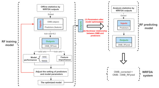
Figure 1.
Flowchart of the RF model coupling with the WRFDA system for the bias correction of satellite radiances.
Secondly, once the model optimal parameters have been confirmed, the nonlinear relationship between the OMB departures and several predictors fitted by the RF training model will be inherited to the RF predicting model. Meanwhile, the predictors from testing datasets valid at the analysis time will be extracted as inputs to the RF prediction model. Then, the outputs of the RF prediction model denoted as OMB_RFpred in Figure 1 are applied as the estimates of the systematic bias for the radiance data assimilation in the WRFDA system. The final prediction of OMB_RFpred is made based on the mean of all predictions from each individual tree on test samples , as,
where T is the total number of regression trees.
2.4. Experimental Design
Three parallel experiments are designed to evaluate the impact of different BC schemes for AGRI channels 9–10 under clear-sky. These experiments differ in predictors and BC algorithms with their detailed configurations shown in Table 1. The RF_pre4 and RF_pre7 experiments are configured consistently with the same nonlinear correction method of RF but differ in the settings of BC predictors. Unlike the other experiments, Linear_pre7 uses a linear solver of the least square fitting to correct the OMB biases. Apart from the traditional predictors p0–p4, the predictors p5—longitude, p6—scene brightness temperature, and p7—scan position (scan pixels number in the latitudinal direction) are additionally used for the RF_pre7 and Linear_pre7 experiments. The three newly added predictors p5–p7 are more sensitive to the OMB biases as shown in Section 3.2.1. Predictors p1–p4 generally depend on the atmospheric state, while predictors p5–p7 are to allow for representing the bias characteristics of the satellite observations.

Table 1.
The setting of three experiments.
For all the experiments, the statistical correlations based on both the linear and nonlinear methods are obtained on a representative set of OMBs and predictors over the domain. The local area concerned is covering from the west of China to the western Pacific Ocean (15°N–55°N, 90°E–140°E) centered at 35°N, 115°E, where the “21·7” Henan extremely heavy rainfall occurred. The offline statistics are generated by the WRF-3DVar system based on the datasets of National Centers for Environmental Prediction (NCEP) operational 0.25° × 0.25° Global Forecast System (GFS) analysis and the full disk FY-4A AGRI observations. The training sets are available from 1800 UTC 4 July 2021 to 1800 UTC 18 July 2021, every 6 h. As for the RF predicting model, the testing datasets are valid at 0600 UTC 19 July 2021. The background is generated from a 6-h spin-up forecast as the cold starts.
Successful radiance assimilation requires high-quality datasets for the RF model and the WRFDA system. The following four steps of quality control (QC) are adopted in all the experiments, including (1) rejecting all channels with mixture surface types of observation data; (2) rejecting the satellite zenith angels are larger than 60°; (3) rejecting the observations if the absolute OMB innovation exceeds 3 times the observation error under clear-sky conditions, and if it exceeds 15 K; (4) for the clear-sky radiance data assimilation, rejecting the cloudy pixels with a Particle Filter (PF) cloud detection scheme proposed by Xu et al. (2016) [40].
3. Results
3.1. Predictive Capability of RF Model
The optimal parameters can be confirmed based on the error metrics of out-of-bag data (OOBD) without cross-validations, which is a highly efficient way to assess the model generalization capability for the operational forecast. In each round of bootstraping, about one-third of the training sets called “out-of-bag data” are left out and averaged as an out-of-bag score (OOBS) when the “bootstrap” is set to true. The details of model optimization are described as following.
To optimize the RF model, the model predictive capability is evaluated by adjusting the model configurations in terms of parameters and features. Figure 2 shows the OOBS based on the different model parameters (number and depth of trees). A larger OOBS indicates better predictive capability. As shown in Figure 2a, the OOBS for channel 9 is significantly increased until the depth reaches 25, when the number of trees is 130. Moreover, the trees numbers from 180 to 220 obtain a higher score when the depth of trees is smallest. In Figure 2b, a relatively higher score is found after the depth reaches 30 for the number 170. Accordingly, we set 180 trees and a maximum depth of 25 for channel 9 and 170 trees and 30 depth for channel 10, respectively, to avoid the over-fitting issue. Based on the optimal parameters, the predictors in the first analysis valid at 0600 UTC 19 July 2021 are formed as the new inputs, to obtain the OMB_RFpred through the RF predicting model.
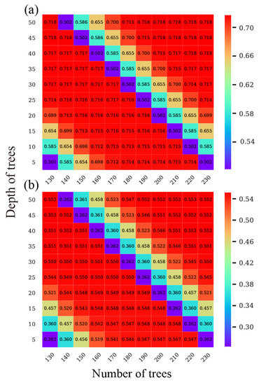
Figure 2.
Out-of-bag score (OOBS) map of RF training model with different model parameters (number and depth of trees) for (a) channel 9 and (b) channel 10. The horizontal axis represents the number of trees, and the vertical axis represents the depth of trees. The sum of OOBSs is 1.
As a premise, it is of great importance to diagnose the contributions of each predictor, whether in the proposed scheme or in the traditional BC schemes. Figure 3 illustrates the feature importance of several predictors for AGRI channel 9 and channel 10, respectively, in the RF training model. The model normalized the feature importance so that the sum of all importance scores is 1. The higher the score, the greater the correlation between predictors and OMB biases. It is evident that the predictors of scene brightness temperature, scan position, and longitude contribute more to the RF model compared to other traditional predictors. Moreover, the importance score of the scene brightness temperature is significantly higher than the other predictors for both AGRI channels 9 and 10.
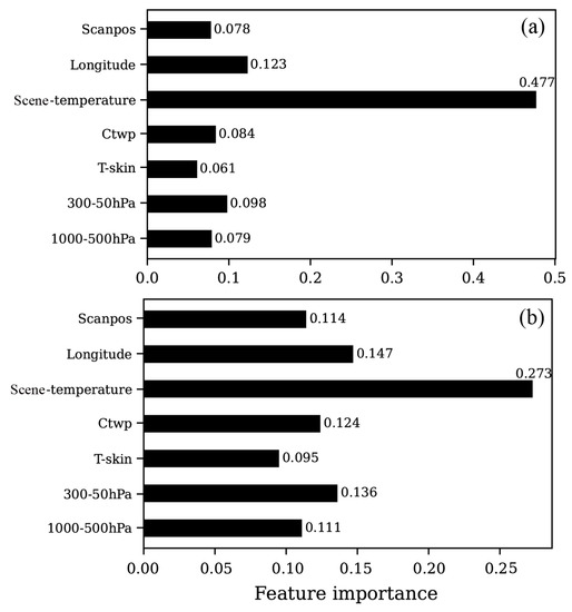
Figure 3.
Feature Importance of the applied predictors in the RF model for AGRI (a) channel 9 and (b) channel 10. The sum of all importance scores is 1.
To evaluate the predictive capability of the RF model, the differences between the real OMB and the predicted OMB from validation sets are measured using the mean absolute error (MAE) and root mean squared error (RMSE) for two experiments with two different bundles of predictors. One bundle consists of predictors p0–p4 and the other includes predictors p0–p7 for BC. As is shown in Table 2, the MAE and RMSE scores of RF_pre7 for AGRI channels 9–10 are significantly lower than those of RF_pre4. The results indicate a strong generalization capability of the RF model based on the extended predictors. The statistical dependence of OMB on the newly added three predictors p5–p7 will be further investigated in the next sections for a better understanding of the model performance. It is worth noting that the error scores for channels 9–10 are rather different. This is probably due to the fact that the statistics are calculated based on the datasets with different data counts. To be specific, the data of channel 10 are more likely to be eliminated by the quality control processes due to the influence of the surface emissivity.

Table 2.
The RF model prediction scores of two different experiments.
3.2. Comparison of Different BC Schemes
The comparison of three experiments is elaborated in this section to assess the performance of linear and nonlinear BC schemes in the assimilation of the observations of AGRI channels 9–10. Meanwhile, the contribution of those additional predictors p5–p7 to the BC effectiveness will be further evaluated by adding the sensitivity experiments in the framework of the same BC method.
3.2.1. Variations in Bias with Predictors
The OMB biases are characterized with the nonlinearity variations along with several predictors. As seen from Figure 4, the biases of OMB noticeably increase as the p5 scene brightness temperature (scene temperature) increases in all the experiments except for the RF_pre7, especially when the scene temperature is less than 238 K (250 K) for channel 9 (channel 10). The OMB_noBC results without BC have a large amplitude of more than 6 K for both AGRI channels. An apparent scene temperature-dependence bias of OMB exits in the OMB_noBC, RF_pre7 and Linear_pre7 experiments, caused by the instrument nonlinearity. The practical nonlinearity problem is an important factor affecting the calibration accuracy of infrared imaging instruments [41]. As expected, the nonlinear correction ability of RF would be desirable to overcome this assimilation issue when taking p5–p7 as one of the predictors. The OMB biases of AGRI channels 9–10 in RF_pre7 are both weak or negligible dependent on the scene temperature according to the smallest variation amplitude in a range of −2 K to 2 K.
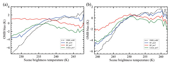
Figure 4.
Variations in the biases of OMB (unit:K) with respect to the predictors of scene brightness temperature (unit: K) for AGRI (a) channel 9 and (b) channel 10 valid at 0600 UTC 19 July 2021.
Variations in the OMB biases with respect to the predictors of longitude is elaborated for AGRI channels 9–10 in Figure 5. A finite range of values for the scan position and longitude is relevant to the regional statistics applied for the limited-area model of the WRFDA system (Figure 5 and Figure 6). The biases variation along with the longitude display relatively small fluctuations near 0 K in the RF_pre4 experiment compared to those from other experiments, especially for the AGRI channel 9. The Linear_pre7 and OMB_noBC results show a clearly negative bias with an amplitude of more than 1 K and 2 K, respectively. In the region from 100°E to 130°E, the corrected bias from the RF_pre7 experiment is rather significant. Furthermore, it is found that the bias correction effects are different between channel 9 and channel 10. A possible reason is that the predictive capability of the RF model for channel 9 and channel 10 is different, as shown in Table 2.
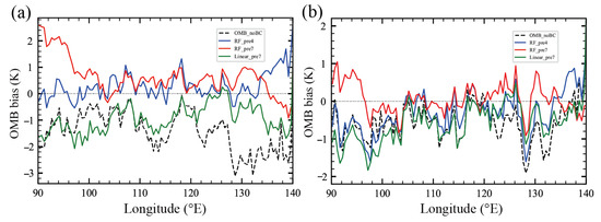
Figure 5.
Variations in the OMB biases (unit: K) with respect to the predictors of longitude for AGRI (a) channel 9 and (b) channel 10 valid at 0600 UTC 19 July 2021.
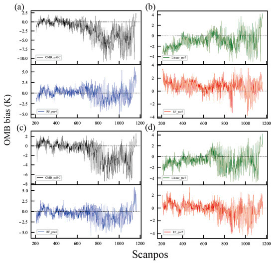
Figure 6.
Variations in the average OMB biases (unit: K) with respect to the predictors of scan position (pixels number of latitudinal direction) from the different experiments for AGRI (a,b) channel 9 and (c,d) channel 10, respectively, valid at 0600 UTC 19 July 2021. (a,c) The left panels represent the comparison between the OMB_noBC (black lines) and RF_pre4 (blue lines) experiments. (b,d) The right panels represent the comparison between the OMB_noBC (black lines) and RF_pre4 (blue lines) experiments.
The OMB biases before BC exhibit negative biases of AGRI channels 9–10 along with the latitudinal scan position values from 700 to 1100 (Figure 6a,c). It seems that these cold biases are efficiently revised by the RF method since the corrected biases are mostly closer to 0 K in the RF_pre4 and RF_pre7 experiments in Figure 6. Nevertheless, the cold biases still partly exist in the experiments of Linear_pre7. As is well known, the assimilation of undetected cloudy pixels will likely lead to a cooling observed field, for which the OMB biases are negative for the infrared radiances [42]. Results indicate that the nonlinear correction scheme has the potential ability to account for the prevalence of nonlinear biases caused by clouds.
3.2.2. OMB Distributions
Figure 7 shows the QC-passed scatters of the simulated brightness temperature (B) versus the observed brightness temperature (O) before and after the BC for AGRI channel 9 and channel 10 radiance data along with the density distribution of pixels. It can be seen that the mean of the OMB is notably large before BC, which is effectively reduced by all the experiments except for channel 10 in the Linear_pre7 experiment. The best agreement between the observation and the background after BC is provided by the RF-based experiments, with the smallest OMB mean nearly at 0.233 K for channel 9 and 0.105 K for channel 10. Additionally, the scatter distribution of RF_pre7 around the isoline is denser than the other experiments (Figure 7c,g). It is noted that the standard deviation (std) of corrected-OMBs in the experiments of RF_pre7 and Linear_pre7 are smaller than those from the experiments with only the predictors p0–p4.
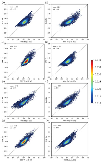
Figure 7.
The QC-passed scatters of observed versus RTTOV-calculated brightness temperature (unit: K) from the background (a) before BC, (b) after BC with RF_pre4, (c) after BC with RF_pre7, and (d) after BC with Linear_pre7 for AGRI channel 9. The scatters of observed (OBS Tb) versus RTTOV-calculated brightness temperature (unit: K) from the background (BAK Tb) (e) before BC, (f) after BC with RF_pre4, (g) after BC with RF_pre7, and (h) after BC with Linear_pre7 for AGRI channel 10. The proportions of data counts are indicated as the shading.
The probability density function (PDF) of the normalized OMB is shown in Figure 8 based on different BC schemes after the quality control. Approaching the Gaussianity distribution (black dotted curves) is expected to statistically lead to more accurate analyses. The kurtosis of OMB distributions before BC (orange curves) are obviously sharper than the Gaussian curve. As compared to the reference, the positive skewness of OMB_noBC is symmetrically shifted to near 0 K by all the BC experiments for both AGRI channels. However, it is observed that the OMB from Linear_pre7 experiment displays too-pronounced peaks at the left tails near around −2 K, as is marked with the black boxes. This cold departure is probably corresponding to the cloudy pixels not being completely rejected. On the contrary, the frequencies of OMB from the RF_pre7 and RF_pre4 experiments match the Gaussian distribution relatively better, especially for those left tails. All the results suggest that the RF method is capable of measuring the nonlinear relationship between the OMB biases and the BC predictors.
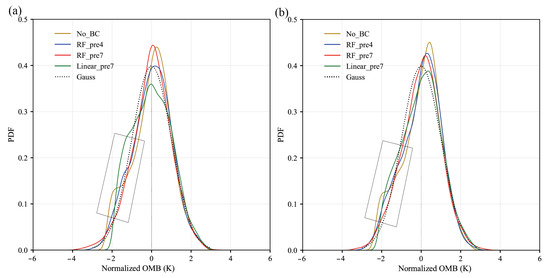
Figure 8.
Probability density function (PDF) of normalized OMB departures before BC (orange curves) and after BC from the experiments of RF_pre4 (blue curves), RF_pre7 (red curves), and Linear_pre7 (green curves), respectively, versus the Gaussian distribution (black dotted curves) for AGRI (a) channel 9 and (b) channel 10.
In addition, the brightness temperature (BT) distributions of OMBs for AGRI channels 9–10 are illustrated with and without the BC by comparing the experiments of RF_pre7 and Linear_pre7 (Figure 9). It can be seen that the OMB BT distribution without the BC in Figure 9a,b shows large negative biases and positive biases in some areas, which could be modified by the BC experiments of RF_pre7 and Linear_pre7, respectively. However, there is a significant cold bias of OMB BT in the Linear_pre7 experiment, especially over the continental area (Figure 9e,f). This is consistent with the finding of more negative OMB biases from Linear_pre7, indicated by the black boxes dotted in Figure 8. In contrast, those cold biases have been removed to some extent in the RF_pre7 experiment (Figure 9c,d). The otherness of OMB BT distributions from RF_pre7 is relatively insignificant, with a smaller std of OMB against the linear experiments.
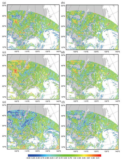
Figure 9.
The brightness temperature (unit: K) distributions of the observation minus the background (OMB) before the bias correction for AGRI (a) channel 9 and (b) channel 10, after the bias correction from the RF_pre7 experiment for AGRI (c) channel 9 and (d) channel 10, and from the Linear_pre7 experiment for AGRI (e) channel 9 and (f) channel 10, valid at 0600 UTC 19 July 2021.
3.2.3. Verification of Analyses
It is important to verify the potential effects of different BC methods on the subsequent assimilation of AGRI radiances. If the model background or observations contains systematic errors, the analysis will diverge from the true state [43]. Figure 10 and Figure 11 show the bias and root-mean-square error (RMSE) vertical profiles of the analyses verified against a set of conventional observations (sounding and surface synoptic). The dots marked in Figure 10 and Figure 11 show the results above a 95% significant level.
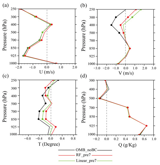
Figure 10.
The bias vertical profiles of the analyses with the radiances of AGRI channels 9–10 from the OMB_noBC (black lines), RF_pre7 (red lines), and Linear_pre7 (green lines) experiments, respectively, verified against the sounding and surface synoptic observations for (a) U-wind, (b) V-wind, (c) temperature, and (d) specific humidity valid at 0600 UTC 19 July 2021. The marked dots show a significance level above 95%.
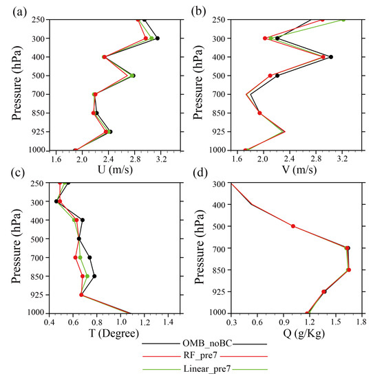
Figure 11.
The root-mean-square error (RMSE) vertical profiles of the analyses with the radiances of AGRI channels 9–10 from the OMB_noBC (black lines), RF_pre7 (red lines), and Linear_pre7 (green lines) experiments, respectively, verified against the sounding and surface synoptic observations for (a) U-wind, (b) V-wind, (c) temperature, and (d) specific humidity valid at 0600 UTC 19 July 2021. The marked dots show a significance level above 95%.
Among the results of different BC experiments, the best initial estimate is achieved by the proposed RF_pre7 scheme with the smallest bias for all variables at almost all levels, except for a slightly positive impact on the temperature analyses at the higher levels above 400 hPa (Figure 10). However, the Linear_pre7 scheme is not as effective as the nonlinear scheme in the improvements of the initial conditions. Figure 11 displays the consistent conclusions as Figure 10 but for the verification metrics of RMSE. The results suggest that the analyses after BC are generally improved for the synoptic variables, though the RF nonlinear scheme has a little direct impact on the reduced RMSE of analyses for specific humidity, as shown in Figure 11d. Yet, in the RF_pre7 experiment, the variables of winds and temperatures below 400 hPa show some improvements in terms of the reduced RMSE scores (Figure 11a–c).
To further assess the robustness of the RF scheme, the experiments are conducted for another analysis time that is far from the training period. Figure 12 and Figure 13 show the bias and RMSE vertical profiles, same as Figure 10 and Figure 11, but are valid at 0600 UTC 20 July 2021. It is observed that the bias and RMSE scores from Linear_pre7 experiments are characterized by the smallest errors of U-winds in the upper troposphere and higher errors of other variables as a comparison to RF_pre7. The errors in RF_pre7 experiments are generally reduced, especially for the temperature. The smaller errors from the BC experiments relative to the OMB_noBC experiment indicate that the quality of the synoptic variables from analyses could be improved by the BC. Generally, the largest improvements exist in the experiments with the proposed RF scheme.
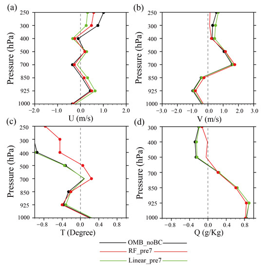
Figure 12.
The bias vertical profiles of the analyses with the radiances of AGRI channels 9–10 from the OMB_noBC (black lines), RF_pre7 (red lines), and Linear_pre7 (green lines) experiments, respectively, verified against the sounding and surface synoptic observations for (a) U-wind, (b) V-wind, (c) temperature, and (d) specific humidity valid at 0600 UTC 20 July 2021. The marked dots show a significance level above 95%.
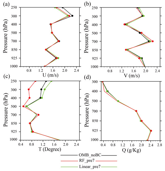
Figure 13.
The root-mean-square error (RMSE) vertical profiles of the analyses with the radiances of AGRI channels 9–10 from the OMB_noBC (black lines), RF_pre7 (red lines), and Linear_pre7 (green lines) experiments, respectively, verified against the sounding and surface synoptic observations for (a) U-wind, (b) V-wind, (c) temperature, and (d) specific humidity valid at 0600 UTC 20 July 2021. The marked dots show a significance level above 95%.
4. Discussion
In this study, a nonlinear BC method based on the RF machine learning technology was developed and implemented in order to remove the nonlinear conditional biases to enhance the efficiency of AGRI radiance data assimilation. Compared with other machine learning technologies, one of the advantages of RF is that it is suitable for high-dimensional datasets and has the capability to evaluate the feature importance of BC predictors. Unlike the traditional BC schemes, such as the VarBC method, the proposed scheme has the advantage of fitting the nonlinear relationship between the predictors and OMB biases to better correct the nonlinear conditional biases.
First, the performance of the RF-based correction model was evaluated with two different settings of BC predictors. According to the results, it is confirmed that the configuration of p0–p7 predictors is able to enhance the generalization capability of the RF model. The additional predictors of p5–p7 were also diagnosed in the RF model as contributing significantly to the prediction of objects. To be specific, the traditional predictors p0–p4 mainly represent the bias characteristics in the model space, while the newly added predictors p5–p7 could reflect the information of observed space errors. Moreover, those results can be explained by the fact that the RF model is suitable for the high-dimensional and multi-feature datasets.
The application effects of the BC nonlinear scheme were investigated and compared with the linear BC scheme for the observations of AGRI channels 9–10. As expected, the OMB biases could be effectively decreased by the RF nonlinear scheme against the linear scheme as well as a more idealized error distribution of OMB shown in the RF-based experiments. The nonlinear BC method based on RF outperforms the linear BC method, especially for correcting the biases of AGRI observation caused by the nonlinear processes. An apparent scene temperature-dependence bias of OMB is observed for AGRI channels 9–10, which is caused by the nonlinearity process of the instrument calibration. Furthermore, the significant negative biases of OMB may be related to a cooling observed field resulting from the simulation of cloudy pixels. The cloud-related processes are generally non-linear and complicated. Thus, the simulation of cloud-related processes is always simplified and linearized in most numerical models, causing non-negligible nonlinear biases.
In addition, according to the verification of analyses, it is speculated that the proposed nonlinear BC scheme with p0–p7 predictors has the potential to increase the quality of the analyses after recognizing the system biases from AGRI observations. All of those results shown in Section 3 suggest that identifying the nonlinear correlations among the OMB and the predictors through the RF method is conducive to BC with the subsequent positive impacts on data assimilation.
5. Conclusions
BC is an essential step to remove the systematic biases before radiance data assimilation. In this study, the AGRI clear-sky observations from channels 9–10 were utilized to explore the ability of a nonlinear BC method based on the RF technology in the WRF-3DVar system. The experiments are conducted using a comparative assessment, using a traditional linear method as the benchmark to assess the proposed RF scheme performance. According to the feature importance of BC predictors, two different settings of BC predictors are designed in order to further enhance the application effect of the RF model.
It is found that the configuration of predictors p0–p7 provides a consistent improvement in systematic bias correction. Utilizing the newly added predictors p5–p7 based on the RF nonlinear method may effectively contribute to the reduced scene temperature-dependent biases. The mean and std of OMB with the RF scheme are significantly decreased in comparison to the traditional linear scheme. Further, the proposed nonlinear scheme yields an optimized estimate of the real atmospheric state by taking advantage of the reduced system biases of AGRI channels 9–10.
Despite the above encouraging results, more efforts will be extended to assess the positive impact on data assimilation from the infrared observations, upgrading the numerical forecasting skill by applying the machine learning method in the procedure of BC. On the other hand, the inherent nonlinear interactions are largely found in the cloud-related processes between the local thermodynamic environment and various cloud hydrometers. Thus, nonlinear BC methods are also planned for the all-sky radiance data assimilation.
Author Contributions
Conceptualization, D.X.; writing—original draft, X.Z. and D.X.; writing—review and editing, X.L. and F.S.; formal analysis, X.Z.; F.S. and D.X.; data curation, X.Z. and X.L.; All authors have read and agreed to the published version of the manuscript.
Funding
This research was funded by the National Key R&D Program of China (2022YFC3080500), the Chinese National Natural Science Foundation of China (G42192553), Program of Shanghai Academic/Technology Research Leader (21XD1404500), the Shanghai Typhoon Research Foundation (TFJJ202107), the Chinese National Natural Science Foundation of China (G41805016), the research project of the Institute of Atmospheric Environment, China Meteorological Administration, Shenyang in China (2020SYIAE02), Postgraduate Research & Practice Innovation Program of Jiangsu Province. We acknowledge the High Performance Computing Center of Nanjing University of Information Science & Technology for their support of this work.
Data Availability Statement
The FY-4A AGRI radiance data were freely downloaded from http://satellite.nsmc.org.cn accessed on 18 December 2021, along with the conventional observations from National Centers for Environmental Prediction (NCEP) operational Global Telecommunication System (GTS) from http://rda.ucar.edu/datasets/ds337.0/ accessed on 18 December 2021. Part of the software was associated with the National Center for Atmospheric Research (NCAR) using version 4.3 of WRF and WRF-3DVar system. The reanalysis is provided by the NCEP Global Forecast System products of the 0.25° × 0.25° GFS datasets, available at https://rda.ucar.edu/datasets/ds0.841/ accessed on 1 December 2021. Figures were made with NCL version 6.6.2 from https://ncl.ucar.edu and Python version 3.3.8 from https://www.python.org accessed on 8 July 2022.
Acknowledgments
We acknowledge the High Performance Computing Center of Nanjing University of Information Science & Technology for their support of this work.
Conflicts of Interest
The authors declare no conflict of interest.
References
- Honda, T.; Kotsuki, S.; Lien, G.-Y.; Maejima, Y.; Okamoto, K.; Miyoshi, T. Assimilation of Himawari-8 All-Sky Radiances Every 10 Minutes: Impact on Precipitation and Flood Risk Prediction. J. Geophys. Res. 2018, 123, 965–976. [Google Scholar] [CrossRef]
- Zou, X.; Qin, Z.; Weng, F. Improved Coastal Precipitation Forecasts with Direct Assimilation of GOES-11/12 Imager Radiances. Mon. Wea. Rev. 2011, 139, 3711–3729. [Google Scholar] [CrossRef]
- Xu, D.; Min, J.; Shen, F.; Ban, J.; Chen, P. Assimilation of MWHS radiance data from the FY-3B satellite with the WRF Hybrid-3DVAR system for the forecasting of binary typhoons. J. Adv. Model. Earth Syst. 2016, 8, 1014–1028. [Google Scholar] [CrossRef]
- Benáček, P.; Mile, M. Satellite Bias Correction in the Regional Model ALADIN/CZ: Comparison of Different VarBC Approaches. Mon. Wea. Rev. 2019, 147, 3223–3239. [Google Scholar] [CrossRef]
- Eyre, J.R. Observation bias correction schemes in data assimilation systems: A theoretical study of some of their properties. Quart. J. Roy. Meteor. Soc. 2016, 142, 2284–2291. [Google Scholar] [CrossRef]
- Xu, D.; Liu, Z.; Fan, S.; Chen, M.; Shen, F. Assimilating all-sky infrared radiances from Himawari-8 using the 3DVar method for the prediction of a severe storm over north China. Adv. Atmos. Sci. 2021, 38, 661–676. [Google Scholar] [CrossRef]
- Eyre, J.R. A bias correction scheme for simulated TOVS brightness temperatures. ECMWF Tech. Memo. 1992, 186, 34. [Google Scholar]
- Harris, B.A.; Kelly, G. A satellite radiance-bias correction scheme for data assimilation. Quart. J. Roy. Meteor. Soc. 2001, 127, 1453–1468. [Google Scholar] [CrossRef]
- Shen, F.; Min, J. Assimilating AMSU-A Radiance Data with the WRF Hybrid En3DVAR System for Track Predictions of Typhoon Megi (2010). Adv. Atmos. Sci. 2015, 32, 1231–1243. [Google Scholar] [CrossRef]
- Watts, P.D.; McNally, A.P. Identification and Correction of Radiative Transfer Modeling Errors for Atmospheric Sounders: AIRS and AMSU-A; ECMWF: Reading, UK, 2004; pp. 23–28. [Google Scholar]
- Dee, D.P. Variational bias correction of radiance data in the ECMWF system. In Proceedings of the ECMWF Workshop on Assimilation of High Spectral Resolution Sounders in NWP, Berkshire, UK, 28 June–1 July 2004; pp. 97–112. [Google Scholar]
- Dee, D.P.; Uppala, S. Variational bias correction of satellite radiance data in the ERA-Interim reanalysis. Quart. J. Roy. Meteor. Soc. 2009, 135, 1830–1841. [Google Scholar] [CrossRef]
- Xu, D.; Zhang, X.; Li, H.; Wu, H.; Shen, F.; Shu, A.; Wang, Y.; Zhuang, X. Evaluation of the Simulation of Typhoon Lekima (2019) Based on Different Physical Parameterization Schemes and FY-3D Satellite’s MWHS-2 Data Assimilation. Remote Sens. 2021, 13, 4556. [Google Scholar] [CrossRef]
- Zhu, Y.; Derber, J.; Collard, A.; Dee, D.; Treadon, R.; Gayno, G.; Jung, J.A. Enhanced radiance bias correction in the National Centers for Environmental Prediction’s Gridpoint Statistical Interpolation data assimilation system. Quart. J. Roy. Meteor. Soc. 2014, 140, 1479–1492. [Google Scholar] [CrossRef]
- Auligné, T.; McNally, A.P.; Dee, D.P. Adaptive bias correction for satellite data in a numerical weather prediction system. Quart. J. Roy. Meteor. Soc. 2007, 133, 631–642. [Google Scholar] [CrossRef]
- Fertig, E.J.; Baek, S.-J.; Hunt, B.R.; Ott, E.; Szunyogh, I.; Aravéquia, J.A.; Kaknay, E.; Li, H.; Liu, J. Observation bias correction with an ensemble Kalman filter. Tellus A 2009, 61, 210–226. [Google Scholar] [CrossRef]
- Han, W.; Bormann, N. Constrained adaptive bias correction for satellite radiances assimilation in the ECMWF 4D-Var. In Proceedings of the EGU General Assembly 2016, Vienna, Austria, 7–22 April 2016. [Google Scholar]
- Okamoto, K.; Sawada, Y.; Kunii, M. Comparison of assimilating all-sky and clear-sky infrared radiances from Himawari-8 in a mesoscale system. Quart. J. Roy. Meteor. Soc. 2019, 145, 745–766. [Google Scholar] [CrossRef]
- Otkin, J.-A.; Potthast, R. Assimilation of All-Sky SEVIRI Infrared Brightness Temperatures in a Regional-Scale Ensemble Data Assimilation System. Mon. Weather Rev. 2019, 147, 4481–4509. [Google Scholar] [CrossRef]
- Honda, T.; Miyoshi, T.; Lien, G.-Y.; Nishizawa, S.; Yoshida, R.; Adachi, S.; Terasaki, K.; Okamoto, K.; Tomita, H.; Bessho, K. Assimilating All-Sky Himawari-8 Satellite Infrared Radiances: A Case of Typhoon Soudelor (2015). Mon. Weather Rev. 2018, 146, 213–229. [Google Scholar] [CrossRef]
- Minamide, M.; Zhang, F. Assimilation of All-Sky Infrared Radiances from Himawari-8 and Impacts of Moisture and Hydrometer Initialization on Convection-Permitting Tropical Cyclone Prediction. Mon. Weather Rev. 2018, 146, 3241–3258. [Google Scholar] [CrossRef]
- Otkin, J.A.; Potthast, R.; Lawless, A.S. Nonlinear Bias Correction for Satellite Data Assimilation Using Taylor Series Polynomials. Mon. Weather Rev. 2018, 146, 263–285. [Google Scholar] [CrossRef]
- Lary, D.J.; Remer, L.A.; MacNeill, D.; Roscoe, B.; Paradise, S. Machine Learning and Bias Correction of MODIS Aerosol Optical Depth. IEEE Geosci. Remote Sens. Lett. 2009, 6, 694–698. [Google Scholar] [CrossRef]
- Jin, J.; Lin, H.; Segers, A.J.; Xie, Y.; Heemink, A. Machine learning for observation bias correction with application to dust storm data assimilation. Atmos. Chem. Phys. 2019, 19, 10009–10026. [Google Scholar] [CrossRef]
- Wang, G.; Chen, J.; Dai, J.; Wang, Y. Bias Correction of Brightness Temperatures in Medium-Wave Channel of FY-4A Infrared Hyperspectral GIIRS. INFRARED. 2021, 42, 39–44. [Google Scholar]
- Chen, K.; Fan, X.; Han, W.; Xiao, H. A Remapping Technique of FY-3D MWRI Based on a Convolutional Neural Network for the Reduction of Representativeness Error. IEEE Trans. Geosci. Remote Sens. 2022, 60, 5302511. [Google Scholar] [CrossRef]
- Yang, J.; Ding, S.; Dong, P.; Bi, L.; Yi, B. Advanced radiative transfer modeling system developed for satellite data assimilation and remote sensing applications. J. Quant. Spectrosc. Radiat. Transf. 2020, 251, 107043. [Google Scholar] [CrossRef]
- Xu, L.; Cheng, W.; Deng, Z.; Liu, J.; Wang, B.; Lu, B.; Wang, S.; Dong, L. Assimilation of the FY-4A AGRI clear-sky radiance data in a regional numerical model and its impact on the forecast of the “21·7” Henan extremely persistent heavy rainfall. Adv. Atmos. Sci. 2023, 40, 920–936. [Google Scholar] [CrossRef]
- Qu, J.H.; Zhang, L.; Lu, Q.F.; Zhang, N.Q.; Wang, D. Characterization of bias in FY-4A advanced geostationary radiation imager observations from ERA5 background simulations using RTTOV. Acta Meteorol. Sin. 2019, 77, 911–922. [Google Scholar]
- Zhu, J.; Shu, J.; Guo, W. Biases Characteristics Assessment of the Advanced Geosynchronous Radiation Imager (AGRI) Measurement on Board Fengyun–4A Geostationary Satellite. Remote Sens. 2020, 12, 2871. [Google Scholar] [CrossRef]
- Geng, X.; Min, J.Z.; Yang, C.; Wang, B.; Xu, D. Analysis of FY-4A AGRI radiance data bias characteristics and a correction experiment. Chin. J. Atmos. Sci. 2020, 44, 679–694. [Google Scholar]
- Tang, F.; Zhuge, X.; Zeng, M.; Li, X.; Dong, P.; Han, Y. Applications of the Advanced Radiative Transfer Modeling System (ARMS) to Characterize the Performance of Fengyun–4A/AGRI. Remote Sens. 2021, 13, 3120. [Google Scholar] [CrossRef]
- Zou, X.; Zhuge, X.; Weng, F. Characterization of Bias of Advanced Himawari Imager Infrared Observations from NWP Background Simulations Using CRTM and RTTOV. J. Atmos. Ocean. Technol. 2016, 33, 2553–2567. [Google Scholar] [CrossRef]
- Liu, J.; Xu, L.; Cheng, W.; Wang, B.; Gong, X.; Deng, Z.; Li, D.; Di, D. Bias Characteristics and Bias Correction of GIIRS Sounder onboard FY-4A Satellite for Data. Chin. J. Atmos. Sci. 2022, 46, 275–292. [Google Scholar]
- Barker, D.M.; Huang, W.; Guo, Y.R.; Bourgeois, A.J.; Xiao, Q.N. A Three-Dimensional Variational Data Assimilation System for MM5: Implementation and Initial Results. Mon. Weather Rev. 2004, 132, 897–914. [Google Scholar] [CrossRef]
- Li, X.; Zou, X. Bias characterization of CrIS radiances at 399 selected channels with respect to NWP model simulations. Atmos. Res. 2017, 196, 164–181. [Google Scholar] [CrossRef]
- Liu, Z.; Zhang, F.; Wu, X.; Xue, J. A regional ATOVS radiance-bias correction scheme for radiance assimilation. Acta Meteorol. Sin. 2007, 65, 113–123. [Google Scholar]
- Breiman, L. Random forests. Mach. Learn. 2001, 45, 5–32. [Google Scholar] [CrossRef]
- Menze, B.H.; Kelm, B.M.; Masuch, R.; Himmelreich, U.; Bachert, P.; Petrich, W.; Hamprecht, F. A comparison of random forest and its Gini importance with standard chemometric methods for the feature selection and classification of spectral data. BMC Bioinform. 2009, 10, 213. [Google Scholar] [CrossRef]
- Xu, D.; Auligne, T.; Descombes, G.; Snyder, C. A method for retrieving clouds with satellite infrared radiances using the particle filter. Geosci. Model Dev. 2016, 9, 3919–3932. [Google Scholar] [CrossRef]
- Saunders, R.W.; Blackmore, T.A.; Candy, B.; Francis, P.N.; Hewison, T.J. Monitoring satellite radiance biases using NWP models. IEEE Trans. Geosci. Remote Sens. 2013, 51, 1124–1138. [Google Scholar] [CrossRef]
- Geer, A.J.; Migliorini, S.; Matricardi, M. All-sky assimilation of infrared radiances sensitive to mid- and upper-tropospheric moisture and cloud. Atmos. Meas. Tech. 2019, 12, 4903–4929. [Google Scholar] [CrossRef]
- Dee, D.P. Bias and data assimilation. Quart. J. Roy. Meteor. Soc. 2005, 131, 3323–3343. [Google Scholar] [CrossRef]
Disclaimer/Publisher’s Note: The statements, opinions and data contained in all publications are solely those of the individual author(s) and contributor(s) and not of MDPI and/or the editor(s). MDPI and/or the editor(s) disclaim responsibility for any injury to people or property resulting from any ideas, methods, instructions or products referred to in the content. |
© 2023 by the authors. Licensee MDPI, Basel, Switzerland. This article is an open access article distributed under the terms and conditions of the Creative Commons Attribution (CC BY) license (https://creativecommons.org/licenses/by/4.0/).