Channel Imbalance Calibration Based on the Zero Helix of Bragg-like Targets

Abstract

The calibration of channel imbalances is currently the main concern in polarimetric calibration (POLCAL) since the crosstalk of recent polarimetric synthetic aperture radar (Pol-SAR) systems is lower than −20 dB. The existing channel imbalance calibration method without corner reflectors utilizes both volume-dominated and Bragg-like targets. However, there are two limitations to using volume-dominated targets. One is that the inaccurate selection of volume-dominated areas in the uncalibrated Pol-SAR images has a negative influence on the estimation of cross-polarization (x-pol) channel imbalance, which subsequently impacts the estimation of copolarization (copol) channel imbalance. The other is that there are minimal volume-dominated areas in some special applications of Pol-SAR, such as planetary exploration. Thus, only selecting Bragg-like targets to estimate the values of both transmitting and receiving channel imbalances, which is proposed in this paper, can avoid the uncertainty brought about by selecting other distributed targets in an uncalibrated imaginary. In addition, the reciprocity assumption and characteristics corresponding to H/$\overline{\alpha }$ decomposition are introduced to eliminate the phase ambiguity for the first time. Compared with previous methods, our method had an obvious advantage in terms of universality, since Bragg-like targets are common in the most illuminating areas. The novel method was applied to both the simulated data from the L-band Advanced Land Observing Satellite (ALOS) and C-band GaoFen-3 (GF-3), and to real data with corner reflectors on site. The results from the simulated data showed that the errors of the amplitude and phase estimation were less than 0.5 dB and 5.0° in most topographical features. Meanwhile, the $VV$/$HH$ terms from all trihedral corner reflectors were less than 0.3 dB for amplitude, and 5.5° for phase after calibration by using the estimated channel imbalances.

1. Introduction

Polarimetric Synthetic aperture radar (Pol-SAR) provides many more details of targets compared with single-polarimetric SAR. With the complete and complex scattering matrix of each point in a high-resolution radar image, Pol-SAR is capable of imaging the Earth’s surface at all possible polarizations through antenna synthesis techniques [1]. The inverse physical information from polarimetric decomposition and classification is widely used in observing the Earth surface from several perspectives, including change detection, and the utilization of water resources, land use, biomass, agriculture, and ocean applications [2,3,4,5,6,7].

Polarimetric calibration (POLCAL) can establish the proper relationships between radar images and geophysical parameters by calibrating the channel imbalances and crosstalk expressed in two polarimetric distortion matrices (PDMs) in Pol-SAR images [8]. The corner reflectors with accurately known scattering matrices are the ideal calibrators for estimating the PDMs of an uncalibrated Pol-SAR image [9,10,11], but the high cost and complexity of corner reflectors deployment limit their application to every Pol-SAR image. To reduce the use of corner reflectors and cost savings, the calibration method based on distributed targets are widely applicable and studied. Those methods can be separated into two categories. The first category is those that combine distributed targets for x-pol channel imbalance and crosstalk with man-made point targets for copol channel imbalance, such as the Quegan [12] and Ainsworth algorithms [13]. In order to further reduce the use of the corner reflector, those algorithms have been proposed as the second category that uses only the distributed targets satisfied with some scattering characteristic assumptions. In 2011, Shimada [14] proposed the first calibration method with the use of distributed targets only, in which the three-component Freeman-Durden decomposition [15] was introduced. The model-based POLCAL approach can only be applied to Amazon forests with a majority of highly random volume scattering targets. However, it is impossible to carry out large-scale applications in various terrains due to specific scene limits and man-made factors. Shi [16] proposed the Unitary Zero Helix (UZHEX) algorithm, in which a low helix component of Bragg-like targets could be used to estimate copol channel imbalance, combined with the Ainsworth algorithm to calibrate the channel imbalances and crosstalk by using vegetation areas and Bragg-like targets [17]. The algorithm is widely used in distributed target calibration campaigns [18]. Since the x-pol components of the dense vegetation area are strong and not easily affected by noise, it is generally believed that the volume-scattering-dominated forest area is a kind of ideal distributed target for estimating x-pol channel imbalances and crosstalk. Thus, all of the abovementioned calibration methods using distributed targets only required the participation of vegetation areas.

However, the vegetation area in many Pol-SAR images is insufficient. For example, in some higher-latitude regions, there is no vegetation area dense enough in winter to be used as a distributed target for estimating the channel imbalance. In addition, most of the illuminated areas of deep space exploration, such as the lunar surface, have no vegetation coverage. The assumptions of the above method could be no longer satisfied due to the lack of vegetation areas. So, it can be difficult to estimate the x-pol channel imbalance and crosstalk. Since the crosstalk is stable due to the high isolation (better than 32 dB [19,20,21,22]) in the recent Pol-SAR system, the POLCAL study focuses on the channel imbalance solution.

This paper aims to provide an alternative calibration method based on Bragg-like targets to apply it to images without adequate volume-dominated areas. Bragg-like targets are more common than the volume-scattering dominated region on both the Earth’s surface and the lunar surface, so the proposed method is expected to be applied to more scenes without using vegetation areas. In addition, selecting only Bragg-like targets in an uncalibrated image can reduce the inaccurate estimation caused by the uncertainty of selecting both vegetation areas and Bragg-like targets.

In this paper, we first propose a novel approach to calibrate the transmitting and receiving channel imbalance based on the UZHEX component of Bragg-like areas such as bare soil directly, without other areas needed. It should be noted that the proposed method is not supposed to replace the methods based on corner reflectors since the scattering matrices of corner reflectors are known for certain. Initially, we implement the ENL and $R_{hhvv}$ [17] to select the Bragg-like targets in the uncalibrated images. Then, both the transmitting and receiving channel imbalances are estimated based on the helix constraint and the reciprocity assumptions. The estimation results are finally derived after phase ambiguity elimination and best-fitting filtering. The major innovations of our method can be concluded by the following two perspectives: (1) The transmitting and receiving channel imbalances are estimated by the zero helix constraint of Bragg-like targets simultaneously. (2) The $H/\overline{\alpha }$ decomposition and the first element of the normalized coherence matrix $⟨N_{11}⟩$ are introduced for the first time to eliminate the ambiguity of the phase derived from the iterative results [23,24,25].

This paper is organized as follows. Section 2 describes two distortion models and briefly introduces the calibration method without corner reflectors based on UZHEX. In addition, the estimated error brought by the inaccurate x-pol channel balance is analyzed in this section. Our method is presented in Section 3. In Section 4, two experiments from different pol-SAR systems, including the L-band Advanced Land Observing Satellite (ALOS) and C-band GaoFen-3 (GF-3) datasets, are utilized to show the effectiveness of the proposed method, and the results of the experiments are analyzed. The discussion is presented in Section 5. Section 6 gives the conclusion and future work.

2. Calibration Model and the UZHEX Constraint

2.1. Pol-SAR Distortion Model

As a result of distortion by crosstalk and channel imbalances, the general Sinclair scattering matrix of a target can be given by

$$\left[M\right]=A{\mathrm{e}}^{\mathrm{j}\varphi }\left[R\right]\left[F\right]\left[S\right]\left[F\right]\left[T\right]+\left[N\right]$$

(1)

with

$$\left[M\right]=\left(\begin{array}{cc}{M}_{\mathrm{hh}}& M_{\mathrm{hv}}\\ M_{\mathrm{vh}}& M_{\mathrm{vv}}\end{array}\right)\left[S\right]=\left(\begin{array}{cc}{S}_{\mathrm{hh}}& S_{\mathrm{hv}}\\ S_{\mathrm{vh}}& S_{\mathrm{vv}}\end{array}\right)$$

$$\left[R\right]=\left(\begin{array}{cc}1& {\delta }_2\\ {\delta }_1& f_1\end{array}\right)\left[T\right]=\left(\begin{array}{cc}1& {\delta }_3\\ {\delta }_4& f_2\end{array}\right)$$

$$\left[F\right]=\left(\begin{array}{cc}cos\mathrm{\Omega }& sin\mathrm{\Omega }\\ -sin\mathrm{\Omega }& cos\mathrm{\Omega }\end{array}\right)\left[N\right]=\left(\begin{array}{cc}{N}_{\mathrm{hh}}& N_{\mathrm{hv}}\\ N_{\mathrm{vh}}& N_{\mathrm{vv}}\end{array}\right)$$

$M_{pq}$ and $S_{pq}$ are the measured matrix and true scattering matrix coefficients, respectively, for the polarization $p/q$, which represent different polarimetric channels. A and $\varphi$ are the amplitude and phase of absolute radiation factors, which can be calibrated by using the radiation calibration. $f_1$ is the transmitted channel imbalance, and $f_2$ is the received channel imbalance. ${\delta }_1$, ${\delta }_2$; and ${\delta }_3$, ${\delta }_4$ are the crosstalks of reception and transmission, respectively. $\mathrm{\Omega }$ is the Faraday rotation angle, and N is the system noise. The effect of $\mathrm{\Omega }$ and N can be eliminated according to previous studies [17,26]. It should be noted that the proposed algorithm based only on Bragg-like targets is applied to the system with less or no Faraday rotation angle; for example, the airborne case and the spaceborne PolSAR system whose frequency is C-band or higher than C-band. Therefore, the Faraday rotation angle is ignored in this paper, andthe simplified measured scattering matrix can be formulated by

$$\begin{array}{c}\left[M\right]=A{\mathrm{e}}^{\mathrm{j}\varphi }\left[R\right]\left[F\right]\left[S\right]\left[F\right]\left[T\right]\end{array}$$

(2)

Generally, (2) can be rewritten as [13]:

$$\left[\underline{M}\right]=Y\left[X\right]\left[Q\right]\left[K\right]\left[\underline{S}\right]$$

(3)

with

$$\begin{array}{cc}\hfill \left[X\right]& =\left[\begin{array}{cccc}1& v& w& vw\\ z& 1& wz& w\\ u& uv& 1& v\\ uz& u& z& 1\end{array}\right]\hfill \\ \hfill \left[Q\right]& =\left[\begin{array}{cccc}\alpha & 0& 0& 0\\ 0& 1& 0& 0\\ 0& 0& \alpha & 0\\ 0& 0& 0& 1\end{array}\right]\hfill \\ \hfill \left[K\right]& =\left[\begin{array}{cccc}{k}^2& 0& 0& 0\\ 0& k& 0& 0\\ 0& 0& k& 0\\ 0& 0& 0& 1\end{array}\right]\hfill \end{array}$$

(4)

where $\left[\underline{M}\right]$ and $\left[\underline{S}\right]$ are the vector formats of $\left[M\right]$ and $\left[S\right]$, respectively. $\left[X\right]$, $\left[Q\right]$, and $\left[K\right]$ represent crosstalk, x-pol channel imbalance, and copol channel imbalance, respectively. The new parameters are defined as follows:

$$u={\delta }_{4}v={\delta }_4/f_{1}w={\delta }_3/f_{2}z={\delta }_1$$

(5)

$$k=\frac{1}{f_2}\alpha =\frac{f_2}{f_1}Y=A{f}_1{f}_2$$

(6)

Since $f_1$|$f_2$ and $\alpha$|k can represent channel imbalances in POLCAL, they are utilized in turn for convenience in the following derivation. The uncalibrated covariance matrix is given by

$$\left[O\right]=\left[\underline{M}\right]{\left[\underline{M}\right]}^{\mathrm{H}}=Y\left[X\right]\left[Q\right]\left[K\right]\left[C\right]{\left(\left[X\right]\left[Q\right]\left[K\right]\right)}^{\mathrm{H}}$$

(7)

where $\left[C\right]$ represents the true covariance matrix of a target, and the superscript $\mathrm{H}$ represents the transposed conjugate operator of a matrix.

2.2. POLCAL Methodology without Corner Reflectors Based on UZHEX

A complete workflow ([17], Figure 1) for polarimetric calibration based on the UZHEX without corner reflectors was first proposed. It utilizes the reciprocity and nonsymmetric reflection of natural features, and the zero helix scattering power of bare soil. Before estimating the PDMs, the volume-dominated targets for estimating the crosstalk and x-pol channel imbalance, and Bragg-like targets for inversing the x-pol channel imbalance are separately selected in the uncalibrated Pol-SAR images by ENL and $R_{hhvv}$, which can be estimated by

$$R_{hhvv}=\frac{\left|O_{hhvv}\right|}{\sqrt{O_{hhhh}{O}_{vvvv}}}$$

(8)

$$ENL=\frac{Tr\left\{\left[O\right]\left[O\right]\right\}}{E(Tr{\left\{\left[M\right]{\left[M\right]}^{\mathrm{H}}\right\}}^2)-Tr{\left\{\left[O\right]\right\}}^2}$$

(9)

where $Tr\left\{·\right\}$ represents the matrix trace. It is verified that $R_{hhvv}$ is immune to the distortion factors if the second-order items of the crosstalk can be ignored and the reflection symmetric assumption is satisfied [12,17].

The volume-dominated targets are selected by setting the thresholds of the above two parameters. Although several researchers have proposed methods to estimate crosstalk and x-pol channel imbalance [12,13,27], the most commonly used algorithms are the ZeroAinswoth (AZ) algorithm and the Quegan algorithm [12,13]. The normalized covariance matrix of selected volume-dominated targets by their span is averaged as the input to the above two methods before obtaining the estimated values. After the crosstalk and x-pol channel imbalances are calibrated very well, the covariance matrix is calibrated as [17]

$$\left[\mathrm{\Sigma }\right]={\left(\left[X\right]\left[Q\right]\right)}^{-1}\left[O\right]{\left(\left[X\right]\left[Q\right]\right)}^{-\mathrm{H}}=\left[K\right]\left[C\right]{\left[K\right]}^{\mathrm{H}}$$

(10)

Shi [16] first proposed that the low helix components of Bragg-like targets can be used to calibrate copol channel imbalance. The helix component is defined as follows [28]:

$$\mathrm{Helix}=\Im (⟨(S_{\mathrm{hh}}-S_{\mathrm{vv}})S_{\mathrm{hv}}^{*}⟩)$$

(11)

where $\Im \left(·\right)$ is the imaginary operation. The UZHEX constraint is

$$F(\left[\mathrm{\Sigma }\right],p)=\Im \left(\left|p\right|p{\overline{\mathrm{\Sigma }}}_A+\frac{1}{\left|p\right|}p{\overline{\mathrm{\Sigma }}}_B\right)=0$$

(12)

where $p=k^{-1}$, and

$$\begin{array}{c}{\overline{\mathrm{\Sigma }}}_A={\overline{\mathrm{\Sigma }}}_{\mathrm{Are}}+i·{\overline{\mathrm{\Sigma }}}_{\mathrm{Aim}}=({\mathrm{\Sigma }}_{13}+{\mathrm{\Sigma }}_{12})/2\hfill \\ {\overline{\mathrm{\Sigma }}}_B={\overline{\mathrm{\Sigma }}}_{\mathrm{Bre}}+i·{\overline{\mathrm{\Sigma }}}_{\mathrm{Bim}}=({\mathrm{\Sigma }}_{34}+{\mathrm{\Sigma }}_{24})/2\hfill \end{array}$$

(13)

The estimated values of the copol channel imbalance are the solution to the nonlinear (12) by Newton iteration. Then, the d-fit solution operated to remove the potential deviation is utilized to invert the true covariance matrix by

$$\left[C\right]={\left(\left[K\right]\left[X\right]\left[Q\right]\right)}^{-1}\left[O\right]{\left(\left[K\right]\left[X\right]\left[Q\right]\right)}^{-\mathrm{H}}$$

(14)

2.3. Influence of the X-Pol Channel Imbalance $\alpha$ Estimation Error

For the UZHEX algorithm, the accurate estimation of the copol channel imbalance is based on a precise calibration of the x-pol channel imbalance in a Pol-SAR system with lower crosstalk. The calibration results of crosstalk and x-pol channel imbalance influence the accuracy of the copol channel imbalance estimation. Assuming that $\left[Q^{\prime }\right]$ is the matrix of the estimated x-pol channel imbalance ${\alpha }^{\prime }$ derived from the volume-dominated pixels, it is suggested that $\left[Q^{\prime }\right]$ has a similar format to $\left[Q\right]$. The primarily calibrated covariance matrix (10) can be expressed as follows:

$$\begin{array}{c}\begin{array}{cc}\hfill \left[{\mathrm{\Sigma }}^{\prime }\right]& ={(\left[Q^{\prime }\right])}^{-1}\left[Q\right]\left[K\right]\left[C\right]{\left[K\right]}^{\mathrm{H}}{({(\left[Q^{\prime }\right])}^{-1}\left[Q\right])}^{\mathrm{H}}\hfill \\ \hfill & =\left[\Delta Q\right]\left[K\right]\left[C\right]{\left[K\right]}^{\mathrm{H}}{\left[\Delta Q\right]}^{\mathrm{H}}\hfill \end{array}\end{array}$$

(15)

where $\left[\Delta Q\right]={(\left[Q^{\prime }\right])}^{-1}\left[Q\right]$. The element $\alpha$ is replaced by $\Delta \alpha =\alpha /{\alpha }^{\prime }$, with the meaning of the channel imbalance estimation error. The elements in (13) corresponding to the helix component are given by

$$\begin{array}{cc}\hfill {\mathrm{\Sigma }}_{12}^{\prime }& ={\left|\Delta \alpha \right|}^2{\mathrm{\Sigma }}_{12}{\mathrm{\Sigma }}_{13}^{\prime }=\Delta \alpha {\mathrm{\Sigma }}_{13}\hfill \\ \hfill {\mathrm{\Sigma }}_{24}^{\prime }& =\Delta \alpha {\mathrm{\Sigma }}_{24}{\mathrm{\Sigma }}_{34}^{\prime }={\mathrm{\Sigma }}_{34}\hfill \end{array}$$

(16)

After multiplying both sides of (12) by $\left|p\right|$, it can be derived that

$$\begin{array}{cc}\hfill F(k,{\mathrm{\Sigma }}^{{}^{\prime }})& =\Im (\frac{{\overline{{\mathrm{\Sigma }}_A}}^{{}^{\prime }}}{{\left|k^{{}^{\prime }}\right|}^2{k}^{{}^{\prime }}}+\frac{{\overline{{\mathrm{\Sigma }}_B}}^{{}^{\prime }}}{k^{{}^{\prime }}})\hfill \\ \hfill & =\Im (\frac{{\left|\Delta \alpha \right|}^2{\mathrm{\Sigma }}_{12}+\left|\Delta \alpha \right|{\mathrm{\Sigma }}_{13}}{{\left|k^{{}^{\prime }}\right|}^2{k}^{{}^{\prime }}}\hfill \\ \hfill & +\frac{\left|\Delta \alpha \right|{\mathrm{\Sigma }}_{24}+{\mathrm{\Sigma }}_{34}}{k^{{}^{\prime }}})\hfill \\ \hfill & =0\hfill \end{array}$$

(17)

where $k^{\prime }$ represents the estimated value of the copol channel imbalance. Based on the reciprocity assumptions, that is, $S_{\mathrm{hv}}=S_{\mathrm{vh}}$, we find that ${\mathrm{\Sigma }}_{12}={\mathrm{\Sigma }}_{13}$, ${\mathrm{\Sigma }}_{24}={\mathrm{\Sigma }}_{34}$. Therefore, (17) can be simplified as

$$\Im (\frac{{\left|\Delta \alpha \right|}^2+\Delta \alpha }{{\left|\Delta k\right|}^2\Delta k}{C}_{12}+\frac{\Delta \alpha +1}{\Delta k}{C}_{24})=0$$

(18)

where $\Delta k=k^{\prime }/k$, which represents the copol channel imbalance estimation error. By assuming that $C_{12}=C_{24}$, we can roughly obtain the relation between $\Delta \alpha$ and $\Delta k$ from (18), which can be written by

$$\Delta \alpha \approx {\left(\Delta k\right)}^2$$

(19)

To verify the conclusion of our derivation in (19), a simulated area of bare soil is used for the experiment. The corresponding parameters are listed in Table 1. Before imposing the x-pol channel imbalance on the data, the relationship between $C_{12}$ and $C_{24}$ is tested to confirm our assumption in (19). The mean value of the $C_{12}/\phantom{C_{12}{C}_{24}}{C}_{24}$ amplitude in the simulated data was 0.1187 dB, and the mean value of the phase was −4.262°. Given that it is regarded as the error caused by the algorithm and the improper selection of volume-dominated pixels, $\alpha$ was added to the ideally simulated data.

Table 1. Parameters of simulated Pol-SAR data of bare soil area.

Size of Bare Soil	Frequency	Residual X-Pol Channel Imbalance
		Amplitude	Phase
100 × 100 pixels	1.5 GHz	−1∼1 dB	−30°∼30°

The results are shown in two three-dimensional (3D) scatter diagrams in Figure 1, with the x-axis and y-axis separately representing the amplitude and phase of $\alpha$. The z-axis represents the estimated amplitude error in dB and the estimated phase error in degrees of x-pol channel imbalance inversed by the UZHEX method [17]. The max amplitude error of k is 0.5009 dB, which is shown in Figure 1a in the darkest red color, while the error is shown in the lighter red when it is closer to 0 dB. Similarly, the max phase error is 15.0578°, and the minimum is 0.0090°. All the splashes are mapped in the Z–X plane in Figure 1a and in the Y–Z plane in Figure 1b. The mapped points clearly show that the error in amplitude of k nearly linearly increases as the amplitude of residual $\alpha$ rises, while there is an apparent growth in the phase of the error of k with the increase of the phase of $\alpha$. These projective spots are mapped to the z-axis with red marking lines. There is a slight difference in the thicknesses of the red lines in the coordinate planes. The lines perpendicular to the z-axis are thicker when the error is farther from zero. Therefore, the simulated experiment also indicates that the relationship between the residual $\alpha$ and the error of estimated k is not a perfectly square relation.

Figure 1. Influence of $\alpha$ on the estimation of k by UZHEX. (a) Influence on the amplitude estimation of k; (b) Influence on the phase estimation of k.

In conclusion, both the derivation and simulation results show the general residual $\alpha$ influence on the estimation of k. It is better to propose a method that can solve the transmitting and receiving channel imbalances with bare soil at the same time to minimize the error caused by residual $\alpha$.

3. Received and Transmitted Channel Imbalance Estimation Based on the UZHEX Constraint

In this section, we propose a method to estimate the received and transmitted channel imbalance without corner reflectors based on the zero helix constraint of Bragg-like targets. The proposed method does not require other distributed targets in the illuminating area, except bare soil. The first step in the proposed method is in selecting the Bragg-like targets in the uncalibrated Pol-SAR images, which are later divided into several bins along the range direction. With the helix component defined by Yamaguchi [28], channel imbalances are estimated by using the zero helix component constraint of selected pixels in each range bin. The Ainsworth algorithm is introduced to roughly correct crosstalk, to make the estimation more accurate. The phase ambiguity of the estimated channel imbalance is eliminated before operating the filter on the estimation results. The final least squares lines are derived after the fitting operation. The workflow of our method is shown in Figure 2.

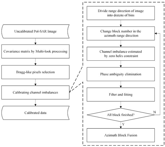
Figure 2. The flowchart of the proposed method.

3.1. Assumptions for the Proposed Method

To develop the calibration algorithm based on Bragg-like targets, several assumptions are made as follows:

• Reciprocity, which is considered as a reasonable hypothesis for most natural targets [12,29]. The reciprocity states that $S_{hv}=S_{vh}$.
• Low helix scattering power for Bragg-like scattering [16,17,30].
• Nonreciprocity for the Pol-SAR radar system. Given that the reciprocity of recently developed polarimetric systems is no longer satisfied [31], we expect that the received modules and transmitted modules are different.
• Range drifting and azimuth nondrifting. The calibration parameters vary with the range direction due to the change of polarization characteristics under the different elevation angle [31], while they are constant in the same range direction due to the short illumination time in each strip [17].

3.2. The Proposed Polarimetric Calibration Framework

3.2.1. Bragg-like Target Selection

Several methods have been proposed to select distributed targets from uncalibrated Pol-SAR images, including deep learning methods [19] and methods based on polarimetric parameters [16,17,18]. Although selecting Bragg-like targets by using a deep learning algorithm is possible, it is limited by the deficiency of a sufficient training set and the cost of the learning process. The traditional polarimetric parameters include ENL, $R_{hhvv}$, and ${\left|C_{22}\right|}^2/\left|C_{11}\right|$. However, the threshold of ${\left|C_{22}\right|}^2/\phantom{{\left|C_{22}\right|}^2\left|C_{11}\right|}\left|C_{11}\right|$ is set differently in each Pol-SAR image, which limits the application of the method. Therefore, the combination of ENL and $R_{hhvv}$ is chosen in the proposed method. The specific details are illustrated in Section 2.2. It is worth noting that it is indeed difficult for calibrators to choose the real targets that show the characteristic of zero helix. However, the subsequent precise mathematical operators for calibration can enlarge the accuracy of the estimated results of $f_1$ and $f_2$.

The Bragg-like targets are selected by [17]

$$R_{hhvv}>R_{upper},ENL>B_{upper}$$

(20)

where $R_{upper}$ and $B_{upper}$ are the thresholds of $R_{hhvv}$ and ENL, respectively. It should be noted that the accuracy of the channel imbalance estimation by our method can be influenced by the accuracy and the number of Bragg-like targets in the uncalibrated Pol-SAR images. In Appendix A, we discuss the detailed influence of the inaccurate selection on the proposed method.

3.2.2. Transmitted and Received Channel Imbalances Calibration

Before estimating the channel imbalances, an uncalibrated Pol-SAR image is divided into several patches in the range direction due to the range drifting properties of the system. The pixels of azimuth are grouped into several blocks, and all blocks have the same solutions when they are in the same patch in the range direction.

In recent Pol-SAR systems, the crosstalk is always low enough to meet the application requirement, and the channel imbalances are the main distortions that need to be calibrated. Thus, we propose an algorithm to estimate the transmitting and receiving channel imbalances based on the UZHEX principle. According to (2) and (7), an uncalibrated Sinclair matrix is distorted by 8 complex values, including crosstalk and channel imbalances. Here, we rewrite the distortion matrix as follows:

$$\left[\underline{M}\right]=A\left[X\right]\left[F_1{F}_2\right]\left[\underline{S}\right]$$

(21)

with

$$\left[F_1{F}_2\right]=\left[\begin{array}{cccc}1& 0& 0& 0\\ 0& f_1& 0& 0\\ 0& 0& f_2& 0\\ 0& 0& 0& f_1{f}_2\end{array}\right]$$

where $\left[F_1{F}_2\right]$ represents the channel imbalances matrix. The uncalibrated covariance matrix can be estimated after multilook processing:

$$\left[O\right]=E(\left[M\right]{\left[M\right]}^H)=\left[X\right]\left[F_1{F}_2\right]\left[C\right]{\left[F_1{F}_2\right]}^H{\left[X\right]}^H$$

(22)

where $E\left(·\right)$ is the mathematical expectation. Since the Sinclair matrix is distorted by the crosstalk and channel imbalances, the reciprocity is not satisfied in $\left[M\right]$, i.e., $M_{hv}\ne M_{vh}$. The helix component can be given by

$$\mathrm{Helix}=\frac{1}{\sqrt{2}}\Im ((C_{12}+C_{13})+(C_{24}+C_{34}))$$

(23)

where $C_{mn}(m=1,2,n=3,4)$ is the element of the real covariance matrix. According to Shi [17], crosstalk is regarded as being less than −20 dB in recent Pol-SAR systems, so that the higher-order term of crosstalk can be ignored. The relationship between $C_{mn}(m=1,2,n=3,4)$ and $O_{mn}(m=1,2,n=3,4)$ can be represented by:

$$\begin{array}{cc}\hfill & C_{12}\approx \frac{-z^{*}{O}_{11}+O_{12}-v{O}_{22}-w{O}_{32}-w^{*}{O}_{14}}{f_1^{*}}\hfill \\ \hfill & C_{13}\approx \frac{-u^{*}{O}_{11}+O_{13}-v{O}_{23}-w{O}_{33}-u^{*}{O}_{14}}{f_2^{*}}\hfill \\ \hfill & C_{24}\approx \frac{-u^{*}{O}_{22}+z^{*}{O}_{23}+O_{24}-z{O}_{14}-w{O}_{44}}{{\left|f_1\right|}^2{f}_2^{*}}\hfill \\ \hfill & C_{34}\approx \frac{-u^{*}{O}_{32}-z^{*}{O}_{33}+O_{34}-u{O}_{14}-v{O}_{44}}{{\left|f_2\right|}^2{f}_1^{*}}\hfill \end{array}$$

(24)

Equation (24) shows that the helix component of the uncalibrated covariance matrix is influenced by both channel imbalances and crosstalk. To estimate $f_1$ and $f_2$ accurately, the Ainsworth method is introduced to eliminate the influence of crosstalk. However, given that the practical x-pol scattering components $C_{22}$ and $C_{33}$ of Bragg-like targets are weak so that they are easily affected by noise, the estimation of crosstalk in our method is not regarded as the real crosstalk of the Pol-SAR image. It should be noted that the crosstalk estimation procedure helps to improve the accuracy of the channel imbalance solution by calibrating part of the crosstalk, rather than eliminating it completely. Therefore, the entire solving process includes two iterations. One of them is the Gauss-Newton iterative algorithm, which is used to calculate the channel imbalances initially. After the results are applied to roughly calculate the crosstalk, the uncalibrated covariance matrix is corrected by the estimation of both channel imbalances and crosstalk. Then, the primarily calibrated data are input into the Gauss-Newton iterative algorithm again to update the estimation results. Finally, the iteration is ended by the threshold by users. The specific iterative processes are introduced in the following.

By assuming that $u,v,w$ and z are zero in (24), the channel imbalances are first estimated with the zero helix component constraint. The helix components, which are related to the observed covariance matrix $\left[O\right]$, $f_{ZHEX}$, can be given by:

$$\begin{array}{cc}\hfill f_{ZHEX}& =\frac{1}{\sqrt{2}}\Im ({p_1}^{*}{O}_{12}+{p_2}^{*}{O}_{13}+{\left|p_2\right|}^2{p_1}^{*}{O}_{24}+{\left|p_1\right|}^2{p_2}^{*}{O}_{34})\hfill \end{array}$$

(25)

where $p_1=1/\phantom{1f_1}{f}_1=a_1+i·b_1$, $p_2=1/\phantom{1f_2}{f}_2=a_2+i·b_2$. Equation (25) is the objective function to invert the channel imbalances. However, when solving $f_{ZHEX}=0$, the solution of $p_1=0$ and $p_2=0$ is an incorrect solution, so that $\left|p_1\right|\left|p_2\right|$ is divided to increase the stability of the proposed method. The UZHEX object function is given by

$$\begin{array}{cc}\hfill f_{UZHEX}& =\Im ((\frac{{p_1}^{*}}{\left|p_1\right|\left|p_2\right|}{O}_{12}+\frac{{p_2}^{*}}{\left|p_1\right|\left|p_2\right|}{O}_{13})+(\frac{\left|p_1\right|{p_2}^{*}}{\left|p_2\right|}{O}_{24}+\frac{\left|p_2\right|{p_1}^{*}}{\left|p_1\right|}{O}_{34}))\hfill \end{array}$$

(26)

To invert $p_1$ and $p_2$ from $f_{UZHEX}=0$, the Gauss-Newton algorithm is used to solve the nonlinear equation. According to the assumption of nondrifting in the azimuth direction, all the pixels in each range bin are distorted by the same channel imbalances so that there are more than 4 observed $\left[O\right]$ in a bin, which are used to solve the Equation (26). Given that the Pol-SAR image has been grouped into several blocks, all of the covariance matrices of the Bragg-like pixels in the same blocks are averaged as the observed matrix to input into the Gauss-Newton iterative algorithm.

In general, the estimation values converge in 10 iterations when the Bragg-like pixels are selected accurately. The estimated values of the channel imbalances correction in (22) are applied as follows:

$$\Gamma ={\left[F_1{F}_2\right]}^{-1}O{\left[F_1{F}_2\right]}^{-H}$$

(27)

According to the assumption of reciprocity, we have $C_{12}=C_{13}$ and $C_{24}=C_{34}$. As mentioned above, since the higher-order term of crosstalk can be ignored, the following formula can be derived:

$$\begin{array}{cc}\hfill & C_{12}\approx -z^{*}{\Gamma }_{11}+{\Gamma }_{12}-v{\Gamma }_{22}-w{\Gamma }_{32}-w^{*}{\Gamma }_{14}\hfill \\ \hfill & C_{13}\approx -u^{*}{\Gamma }_{11}+{\Gamma }_{13}-v{\Gamma }_{23}-w{\Gamma }_{33}-u^{*}{\Gamma }_{14}\hfill \\ \hfill & C_{24}\approx -u^{*}{\Gamma }_{22}+z^{*}{\Gamma }_{23}+{\Gamma }_{24}-z{\Gamma }_{14}-w{\Gamma }_{44}\hfill \\ \hfill & C_{34}\approx -u^{*}{\Gamma }_{32}-z^{*}{\Gamma }_{33}+{\Gamma }_{34}-u{\Gamma }_{14}-v{\Gamma }_{44}\hfill \end{array}$$

(28)

It is clear that (28) has a similar format to that of ([13], (15)). Therefore, ([13], (15)–(19)) are used to solve the update values of crosstalk ${\delta }_u,{\delta }_v,{\delta }_z$, and ${\delta }_w$. Applying the crosstalk correction to $\left[\Gamma \right]$ defines $\left[O^{{}^{\prime }}\right]$ by using the following formula:

$$\left[O^{{}^{\prime }}\right]={\left[\Delta X\right]}^{-1}\left[\Gamma \right]\left[\Delta X\right]$$

(29)

with

$$\left[\Delta X\right]=\left[\begin{array}{cccc}1& {\delta }_v& {\delta }_w& {\delta }_v{\delta }_w\\ {\delta }_z& 1& {\delta }_w{\delta }_z& {\delta }_w\\ {\delta }_u& {\delta }_u{\delta }_v& 1& {\delta }_v\\ {\delta }_u{\delta }_z& {\delta }_u& {\delta }_z& 1\end{array}\right]$$

The elements of $\left[O^{{}^{\prime }}\right]$ are input into (26) to solve the update values of $f_{1\_up}$ and $f_{2\_up}$, with $\left[O\right]$ being replaced by $\left[O^{{}^{\prime }}\right]$:

$$\begin{array}{cc}\hfill {f_{UZHEX}}^{{}^{\prime }}& =\frac{1}{\sqrt{2}}\Im (\frac{{p_{1\_up}}^{*}}{\left|p_{1\_up}\right|\left|p_{2\_up}\right|}{O}_{12}^{{}^{\prime }}+\frac{{p_{2\_up}}^{*}}{\left|p_{1\_up}\right|\left|p_{2\_up}\right|}{O}_{13}^{{}^{\prime }}\hfill \\ \hfill & +\frac{{p_{1\_up}}^{*}}{\left|p_{1\_up}\right|}\left|p_{2\_up}\right|O_{24}^{{}^{\prime }}+\frac{{p_{2\_up}}^{*}}{\left|p_{2\_up}\right|}\left|p_{1\_up}\right|O_{34}^{{}^{\prime }})\hfill \\ \hfill & =0\hfill \end{array}$$

(30)

where $p_{1\_up}=1/f_{1\_up}=a_{1\_up}+i·b_{1\_up}$, and $p_{2\_up}=1/f_{2\_up}=a_{2\_up}+i·b_{2\_up}$.

In summary, the iteration scheme is as follows.

(1)

Solve the $f_{UZHEX}=0$ by the Gauss-Newton iterative algorithm to obtain the initial $f_1$ and $f_2$.

(2)

Produce $\left[\Gamma \right]$ from $\left[O\right]$ by applying the initial estimated $f_1$ and $f_2$.

(3)

Estimate the update values of crosstalk by the Ainsworth method to apply them to the (26), producing $\left[O^{{}^{\prime }}\right]$.

(4)

Solve (25) by using the Gauss-Newton iterative algorithm again to calculate the $f_{1\_up}$ and $f_{2\_up}$ update, $f_{1\_new}=f_{1\_old}{f}_{1\_up}$,$f_{2\_new}=f_{2\_old}{f}_{2\_up}$.

(5)

Rescale crosstalk by $f_{1\_up}$ and $f_{2\_up}$, and return to step 2.

3.2.3. Phase Ambiguity Elimination

It can be proven that there is ambiguity in estimating the phases of $p_1$ and $p_2$. To simplify our demonstration, it is considered that the crosstalk is zero. Equation (26) can be rewritten as

$$\begin{array}{c}\begin{array}{cc}\hfill f_{UZHEX}& =\Im ((\frac{O_{12}}{\left|p_2\right|}+\left|p_2\right|O_{34})exp(-j{\phi }_{p_1})+(\frac{O_{13}}{\left|p_1\right|}+\left|p_1\right|O_{24})exp(-j{\phi }_{p_2}))\hfill \\ \hfill & =\Im (\left|\frac{O_{12}}{\left|p_2\right|}+\left|p_2\right|O_{34}\right|exp(j({\phi }_1-{\phi }_{p_1}))+\left|\frac{O_{13}}{\left|p_1\right|}+\left|p_1\right|O_{24}\right|exp(j({\phi }_2-{\phi }_{p_2})))\hfill \end{array}\end{array}$$

(31)

where ${\phi }_1=Arg(O_{12}/\phantom{O_{12}\left|p_2\right|}\left|p_2\right|+\left|p_2\right|O_{34})$ and ${\phi }_2=Arg(O_{13}/\phantom{O_{13}\left|p_1\right|}\left|p_1\right|+\left|p_1\right|O_{24})$. $Arg\left(·\right)$ represents the phase operation. According to the reciprocity $S_{hv}=S_{vh}$, after squaring the amplitude term and expanding it, the following equations can be easily derived:

$$\left|\frac{O_{12}}{\left|p_2\right|}+\left|p_2\right|O_{34}\right|=\left|\frac{O_{13}}{\left|p_1\right|}+\left|p_1\right|O_{24}\right|$$

(32)

The constraint $f_{UZHEX}=0$ can be simplified as

$$sin({\phi }_1-{\phi }_{p_1})+sin({\phi }_2-{\phi }_{p_2})=0$$

(33)

From (33), the phases of channel imbalances need to satisfy any of the following formulas:

$${\phi }_{+}={\phi }_{p_1}+{\phi }_{p_2}={\phi }_1+{\phi }_2+2m\pi ,m=0,\pm 1,\pm 2\dots$$

(34)

$${\phi }_{-}={\phi }_{p_1}-{\phi }_{p_2}={\phi }_1-{\phi }_2+(2m+1)\pi ,m=0,\pm 1,\pm 2\dots$$

(35)

The above deduction shows that if the results obtained by iteration only satisfy (34)

$$\begin{array}{c}\begin{array}{cc}\hfill {\phi }_{p_1}& =\frac{1}{2}({\phi }_{+}+{\phi }_{-})\hfill \\ \hfill {\phi }_{p_2}& =\frac{1}{2}({\phi }_{+}-{\phi }_{-})\hfill \end{array}\hfill \end{array}$$

(36)

Since the Sinclair matrices of Bragg-like targets meet the reciprocity, the phase of $C_{23}$ in covariance matrix $\left[C\right]$ satisfies $Arg(C_{23})=0$. According to (22), the relation between $C_{mn}(m=1,2,n=3,4)$ and $O_{mn}(m=1,2,n=3,4)$ can be given by

$$C_{23}\approx -u^{*}{O}_{21}-z{O}_{13}+O_{23}-w{O}_{43}-z^{*}{O}_{24}$$

(37)

Since the correlation between the copol scattering component and x-pol scattering component is small enough in the Bragg-like scattering area, (37) can be simplified as:

$$O_{23}\approx f_1{f}_2^{*}{C}_{23}$$

(38)

Thus, combining (38) and $Arg(C_{23})=0$, it can be easily derived that $Arg(O_{23})$ equals ${\phi }_{p_1}-{\phi }_{p_2}$. The phase ambiguity elimination of ${\phi }_{-}$ is as follows.

• Histogram statistics of $Arg(O_{23})$ are performed on the current distance direction, and the peak value is obtained.
• Add or subtract $\pm \pi$ to ${\phi }_{-}$ and compare ${\phi }_{-}\pm \pi$ with ${\phi }_{-}$ to select the value that is closest to the peak value as the accurate estimated ${\phi }_{-}$.

To eliminate the phase ambiguity in ${\phi }_{+}$, $H/\overline{\alpha }$ decomposition [24,25] is introduced to the proposed method. The entropy and parameter $\overline{\alpha }$ are defined by

$$\begin{array}{c}\begin{array}{cc}\hfill H& =-\sum _{i=1}^3{\beta }_i{log}_3{\beta }_i\hfill \\ \hfill \overline{\alpha }& =\sum _{i=1}^3{\beta }_i{\alpha }_i\hfill \end{array}\hfill \end{array}$$

(39)

${\beta }_i$ can be expressed by ${\beta }_i={\lambda }_i/\phantom{{\lambda }_i\sum _{i=1}^3{\lambda }_i}{\displaystyle \sum _{i=1}^3}{\lambda }_i$. ${\lambda }_i$ represents the eigenvalues, and ${\alpha }_i$ depends on the first element of eigenvectors from the coherence matrix $\left[T\right]$. According to Cloude [25], Bragg-like targets are included in Zone 9, i.e., low entropy surface scatter, in the $H-\overline{\alpha }$ plane. Polarimetric entropy and parameter $\overline{\alpha }$ can be estimated by using the normalized mean coherence matrix $\left[N_3\right]$ [23]. The normalized mean coherence matrix $\left[N_3\right]$ was defined by

$$N_3=\frac{\left[T\right]}{Tr\left\{\left[T\right]\right\}}$$

(40)

It was noted that the first element in $N_3$, which is represented as follows, has a similar form to $\overline{\alpha }$ [23]:

$$⟨N_{11}⟩=\sum _{i=1}^3{p}_i{cos}^2{\alpha }_i$$

(41)

From (41) and (39), it is clear that both $\overline{\alpha }$ and $⟨N_{11}⟩$ are related to $p_i$ and ${\alpha }_i$. Combining (41) and (21), distorted $⟨N_{11}⟩$ can be expressed by

$$\begin{array}{c}\begin{array}{cc}\hfill ⟨N_{11}⟩& =\frac{T\left(1,1\right)}{Tr\left\{\left[C\right]\right\}}\hfill \\ \hfill & =\frac{\frac{1}{2}\left({\mathrm{C}}_{11}+{\mathrm{C}}_{41}{\left({\left(f_1{f}_2\right)}^{*}\right)}^2+{\mathrm{C}}_{14}{(f_1{f}_2)}^2+{\mathrm{C}}_{44}{\left|f_1{f}_2\right|}^2\right)}{{\mathrm{C}}_{11}+{\left|f_2\right|}^2{\mathrm{C}}_{22}+{\left|f_1\right|}^2{\mathrm{C}}_{33}+{\mathrm{C}}_{44}{\left|f_1{f}_2\right|}^2}\hfill \\ \hfill & =\frac{\frac{1}{2}\left({\mathrm{C}}_{11}+{\mathrm{C}}_{44}{\left|f_1{f}_2\right|}^2+2\left|C_{14}\right|\left|f_1\right|\left|f_2\right|cos[{\phi }_{14}+{\phi }_{+}]\right)}{{\mathrm{C}}_{11}+{\left|f_2\right|}^2{\mathrm{C}}_{22}+{\left|f_1\right|}^2{\mathrm{C}}_{33}+{\mathrm{C}}_{44}{\left|f_1{f}_2\right|}^2}\hfill \end{array}\end{array}$$

(42)

where ${\varphi }_{14}$ represents the phase of $C_{14}$, and $T\left(1,1\right)$ is the first element in the coherence matrix $\left[T\right]$. After using the estimated amplitude of channel imbalances $\left|f_1\right|$, $\left|f_2\right|$ to preliminarily calibrate $⟨N_{11}⟩$, $⟨N_{11}⟩$ is influenced by ${\phi }_{+}$ only. The x-pol component of the Bragg-like targets is so small that we can derive

$$\begin{array}{c}\frac{1}{2}\frac{C_{11}+C_{44}}{C_{11}+C_{22}+C_{33}+C_{44}}<0.5\end{array}$$

According to Pracks ([32], Figure 4), for Zone 9, i.e., $H<0.5$ and $\overline{\alpha }<42.5$°, it should be satisfied that $⟨N_{11}⟩>0.55$ so that the following should be satisfied:

$$\frac{\left|C_{14}\right|cos[{\phi }_{14}+{\phi }_{+}]}{C_{11}+C_{22}+C_{33}+C_{44}}>0$$

(43)

In conclusion, the ambiguity of ${\phi }_{+}$ can be eliminated by determining the sign of (43).

Although the phase of channel imbalances can be derived from the solution to the simultaneous equations, the ambiguity of $\pm \pi$ still exists in the phases of $f_1$ and $f_2$. The digital elevation model (DEM) [33] and the polarimetric orientation angle (POA) are introduced to eliminate the ambiguity. The ambiguity of the phase can be eliminated [16] by the consistency that the DEM-derived POA and polarimetric data-derived POA should maintain. The Pol-SAR data-derived POA can be written as [34]:

$$\begin{array}{c}\theta =\frac{1}{4}({tan}^{-1}(\frac{{\mathrm{\Omega }}_{23}}{{\mathrm{\Omega }}_{22}+{\mathrm{\Omega }}_{33}})+\pi ))\end{array}$$

(44)

with

$$\begin{array}{cc}\hfill {\mathrm{\Omega }}_{23}& =-\sqrt{2}\Re (C_{12}+C_{13}-C_{42}-C_{43})\hfill \\ \hfill {\mathrm{\Omega }}_{22}& =-\frac{1}{2}(C_{11}-2\Re (C_{14})+C_{44})\hfill \\ \hfill {\mathrm{\Omega }}_{33}& =C_{22}+C_{33}+2\Re (C_{23})\hfill \end{array}$$

It is clear that if the phase of the transmitted channel imbalance adds or subtracts the $\pi$ shift, the phase of the received channel imbalance should subtract or add the $\pi$ shift. Therefore, the consistency of POA can eliminate the ambiguity of the phases by using the DEM information of the illuminating area.

3.2.4. Best-Fit Solution with Filter

According to one of our hypotheses, the distorted parameters vary with the range direction so that the image is divided into several patches along the range direction and several blocks along the azimuth direction before inversing the channel imbalances by the UZHEX method. The filtering and fitting operators are used to obtain more valuable results. The phase filter operation (PFO) and amplitude filter operation (AFO) [16] are modified to derive the linear fitting lines of phases and amplitudes. After finding the main gradient of phase and amplitudes, the coordinate system will be rotated to the main gradient. For phase, there may be three groups according to the histogram of the rotated results in most situations, and the amplitude has one group due to the narrow dispersion [16]. Both of each amplitude and phase group are operated by using a sigma filter, which excludes those for which the absolute values of the biases from the mean value are larger than the standard deviation. To select the more clustered candidates to fit more accurate linear squares lines, the mean value and standard deviation are solved by 85% points around the peak of the histogram, instead of all the points at each group. Then, the candidates selected by the sigma filters are used to fit the best linear model and to obtain the best-fit solution.

3.2.5. Azimuth Block Fusion

The selected number of blocks in the azimuth direction influences the estimation results. According to Shi [16], the fusion operation that puts all of the estimated results from different block numbers, such as 100-, 64-, 32-, 16-, and 0-block, into the PFO and AFO, can relieve the block-dependent problem. Therefore, the same algorithm is used in this paper to obtain the final transmitting and receiving channel imbalance estimation values.

4. Experiments and Results

In this section, we describe two types of experiments undertaken to validate the proposed method, including experiments of simulated data, and real data with trihedral corner reflectors on site. Both the simulated dataset and real dataset were provided by the L-band ALOS satellite and the C-band GF-3 satellite. The estimated channel imbalances from simulated L-band quad-polarimetric data whose imaging area was dominated by Bragg-like targets were provided with different numbers of blocks and fusion results to illustrate the effectiveness of the proposed method. Other simulated data were derived from the GF-3 Quad-polarimetric Stripmap (QPSI) mode data, which were composed of several scenes, including urban, desert, and mountainous areas, to verify the terrain applicability scenes of our method. The real data were also from GF-3 polarimetric data with corner reflectors on site. Additionally, the other calibrated methods of distributed targets are introduced to verify the accuracy of the proposed method. The geographic extent of all the study areas in our experiments is shown in Figure 3, including the terrain and topographic map.

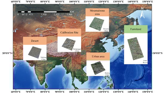
Figure 3. The geographic extent of the study areas on the terrain and topography map. The green box shows the ALOS image, and the red boxes represent the GF-3 images.

4.1. Transmitted and Received Channel Imbalance Estimation with Simulated Data

The real L-band quad-polarimetric image was obtained from the ALOS system with the Phased Array type L-band SAR (PALSAR) onboard, which was launched by the Japan Aerospace Exploration Agency (JAXA) in January 2006. As previous studies have noted [35,36], the residual amplitude imbalance of the published quad-polarimetric product was estimated approximately to be 0.2 dB, and the phase imbalance was estimated to be within 5°. The crosstalk varied from −25 dB to −40 dB. Generally, L-band spaceborne Pol-SAR images are affected by the Faraday rotation angle. The authors in [35,36] describe that the Faraday rotation angle of the Level 1.1 polarimetric products is within 3.5° at different latitudes and at different local times. With those the known prior information, we impose both transmitting and receiving channel imbalances on the standard ALOS polarimetric mode product to artificially simulate the uncalibrated Pol-SAR images. The study area covers Amur in Russia, and the data used in this paper were acquired on 21 April 2011, with a primary size of 18,432 × 1248 in the azimuth and range directions. To maintain consistency with the resolution of the range, the image was operated by a 3-time downsampling process in the azimuth direction so that the image size was changed to 6144 × 1248. The window size is 7 × 7, which is used to estimate the covariance matrix $\left[O\right]$. Figure 4a shows the Pauli decomposition result of the study site. The standard polarimetric data are distorted by the amplitudes of the transmitting and receiving channel imbalances, from −3 dB to 3 dB and 3 dB to −3 dB, respectively, and the phase distortion varies from $-\pi$ to $\pi$ and $\pi$ to $-\pi$, respectively. The Pauli decomposition result after imposing distortion is shown in Figure 4b. We separately set the correlation coefficient $R_{hhvv}$ threshold and ENL as 0.9 and 0.7 in (20) to extract the Bragg-like targets, which are presented in Figure 4c with purple pixels. Each range patch size is 20, and the azimuthal pixels are divided into 100-, 64-, 32-, 16-, and 0-blocks. The final fusion estimation results are used to calibrate the distorted data with the DEM in Figure 4e. The Pauli-RGB image of the calibration result is shown in Figure 4d.

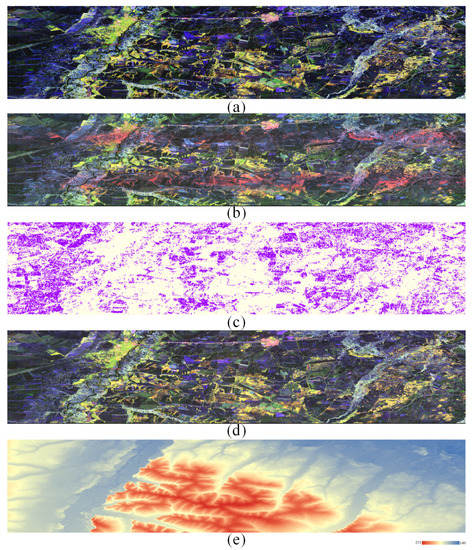
Figure 4. The ALOS dataset. (a) The Pauli-RGB image of real ALOS data; (b) The Pauli-RGB image of simulated distorted ALOS data via channel imbalances; (c) Bragg-like target selection; (d) The recovered Pauli-RGB image after channel imbalances are calibrated; (e) The DEM image of real ALOS data.

In Figure 5 and Figure 6, we display the 100-, 64-, 32-, 16-, 0-blocks, and fusion estimation results of $f_1$ and $f_2$, respectively. The fusion results of the phase are derived after eliminating the $\pm \pi$ phase ambiguity in $f_1$ and $f_2$ via DEM information. Most of the estimated least squares lines (LSLs) in different blocks show a stable consistency with the true value in both the amplitudes and phases of the channel imbalances, which verifies the effectiveness of our method. However, different block numbers indeed influence the accuracy of the estimation. The fusion results are shown in i and j in both Figure 5 and Figure 6 indicate the most stable results compared to other block numbers. Therefore, the fusion results have an obvious advantage from the prospectives of robustness and accuracy.

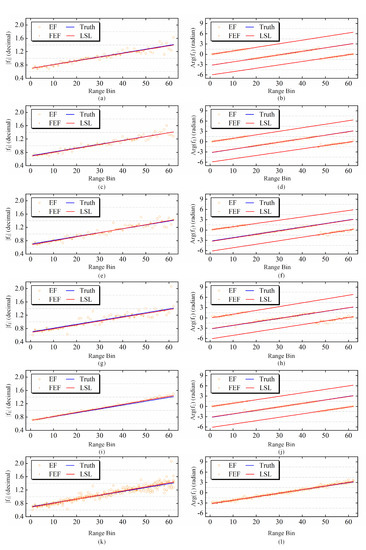
Figure 5. The estimated $f_1$ results of ALOS data. (a,c,e,g,i): The amplitude of the estimated $f_1$ at 100-, 64-, 32-, 16-, and 0-blocks. (b,d,f,h,j): The estimated phase of $f_1$ at 100-, 64-, 32-, 16-, and 0-block. (k,l) The amplitude and phase fusion results of $f_1$ by 100-, 64-, 32-, 16-, and 0-blocks fusion. The estimated channel imbalance (EF) is the result of our method at each range patch, and the filtered estimated channel imbalance (FEF) is derived from the filtered values after AFO and PFO. The truth line and the least squares line (LSL) are linearly fitted by truth values and FEFs, respectively.

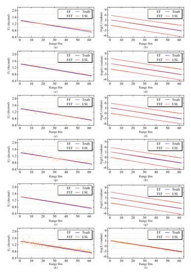
Figure 6. The estimated $f_2$ results of ALOS data. (a,c,e,g,i): The amplitude of the estimated $f_2$ at 100-, 64-, 32-, 16-, and 0-block. (b,d,f,h,j): The estimated phase of $f_2$ at 100-, 64-, 32-, 16-, and 0-block. (k,l) The amplitude and phase fusion results of $f_2$ by 100-, 64-, 32-, 16-, and 0-block fusion.

Since there are a majority of Bragg-like areas in the above illuminating area provided by the ALOS system, it is necessary to confirm the effectiveness in other scenes and other bands. Hence, we collect three typical scenes from the C-band GF-3 QPSI mode with different scenes to demonstrate the applicability of the proposed method. The study areas include urban areas in Beijing, the mountainous area in Liaoning Province, and the Taklimakan Desert in Xinjiang Province in China, whose imaging times are 19 January 2019, 27 May 2019, and 13 June 2019, respectively. Remarkably, sufficiently large homogeneous areas are rarely found in the illuminating areas of mountainous images, which may lead to a greater error in estimating the crosstalk and x-pol channel imbalance. The other data provided by GF-3 are from a desert region in Xinjiang Province in China. In general, the desert is regarded as the region that is dominated by Bragg-like scattering in the C-band. The Pauli-RGB images, Bragg-like target selection images, and DEM of the areas described above are shown in Figure 7.

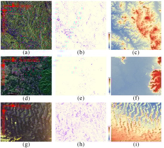
Figure 7. The GF-3 dataset. (a,d,g): The Pauli-RGB image of mountainous area, urban area, and desert in Liaoning Province, Beijing, and Xinjiang Province in China from GF-3 data, respectively; (b,e,h): Bragg-like targets selection images of mountainous area, urban area, and desert, respectively; (c,f,i): The corresponding DEM image.

The window size to suppress the speckle noise and the thresholds of $R_{upper}$ and $B_{upper}$ are the same when processing the ALOS data. The sizes of the three images are 6014 × 7689 for the urban region, 8062 × 6197 for the desert region, and 7550 × 7177 for the mountainous area in the range direction and the azimuth direction. The size of each range bin is 100 in the range direction in the two images, and the azimuth pixels are divided into 100-, 64-, 32-, 8-, and 0-blocks. All of the results of different block numbers are integrated to obtain the fusion results, which are regarded as the final accurate estimation according to the conclusion of the last experiment by the L-band ALOS data. In terms of simulation, the amplitude of −3 dB to 3 dB and the phase of $-\pi$ to $\pi$ are added to the transmitted channel imbalance $f_1$, while the amplitude of 3 dB to −3 dB and the phase of $\pi$ to $-\pi$ are added to the received channel imbalance $f_2$ to verify the accuracy of our method. Table 2 presents the amplitude and phase error after imposing the linear channel imbalances on the real data by using

$$\begin{array}{c}erro{r}_{dB}=\frac{1}{P}{\displaystyle \sum _P}\left|20{log}_{10}\frac{{LSL}_P}{Truth}\right|\hfill \\ erro{r}_{deg}=\frac{1}{P}{\displaystyle \sum _P}\left|Arg({LSL}_P)-Truth\right|\hfill \end{array}$$

(45)

where P represents the number of patches in the range direction.

Table 2. Amplitude (dB) and phase (°) error of $f_1$ and $f_2$ in different sites. The simulated Pol-SAR data are from ALOS and GF-3 systems.

Site	SAR System	Error	100	64	32	16	0	Fusion
Amur Russia	ALOS L-Band	$\Delta \left|f_1\right|$	0.0599	0.0639	0.088	0.1596	0.0873	0.0873
		$\Delta \left|f_2\right|$	0.2407	0.1821	0.1025	0.1100	0.1808	0.1943
		$\Delta Arg(f_1)$	0.7205	1.2585	4.7484	3.0413	1.6378	1.0643
		$\Delta Arg(f_2)$	3.7896	3.6863	3.9199	7.8031	2.7823	3.3845
Xinjiang China	GF-3 C-Band	$\Delta \left|f_1\right|$	0.1303	0.0864	0.0852	0.1011	0.1300	0.1128
		$\Delta \left|f_2\right|$	0.1932	0.2551	0.1535	0.2102	0.3046	0.2127
		$\Delta Arg(f_1)$	1.1770	0.1808	1.6719	0.6361	0.7463	3.8132
		$\Delta Arg(f_2)$	2.7253	1.3765	1.0421	2.9117	3.5738	0.5243
Liaoning China	GF-3 C-Band	$\Delta \left|f_1\right|$	0.1266	0.1209	0.1754	0.2486	0.1505	0.1326
		$\Delta \left|f_2\right|$	0.2501	0.1999	0.2907	0.4362	0.3119	0.2683
		$\Delta Arg(f_1)$	0.7792	0.4788	0.4486	1.0207	0.6840	0.9428
		$\Delta Arg(f_2)$	3.5137	4.1536	3.3257	3.3257	3.2884	3.4584
Beijing China	GF-3 C-Band	$\Delta \left|f_1\right|$	0.5454	0.5085	0.0702	0.4905	0.1026	0.2914
		$\Delta \left|f_2\right|$	0.8424	0.5833	0.2728	0.5729	0.0504	0.3322
		$\Delta Arg(f_1)$	6.3829	5.6142	9.0922	5.2359	4.9939	3.4564
		$\Delta Arg(f_2)$	7.7603	14.2864	9.0450	5.9117	1.7379	1.8388

Table 2 shows that the accuracy of the estimated channel imbalances based on Bragg-like targets is influenced by the scenes. The simulated data in the desert region shows the most accurate results due to the adequate and correct Bragg-like target candidates, which will be used as the original experimental data in the following discussion in the next section. The error provided by the mountainous area and the urban area are larger than that provided by the desert area, because the accuracy of the proposed algorithm depends on both the accuracy of Bragg-like target selection and the number of candidate pixels. The greatest deviation from true value occurs in urban areas, which exceeds 0.5 dB, and 10° when the block number is 100 and 64. However, the fusion error provided by the urban city is within 0.35 dB for the amplitude of channel imbalances, and 3.5° for the phase of channel imbalances.

If we consider that the basic requirements of the Pol-SAR calibration are 0.5 dB in amplitude error and 5° in the phase error of channel imbalance, our algorithm can be applied to the most illuminating areas. According to the above results in different types of scenes, the areas with more natural targets, especially Bragg-like dominated scatters, are given priority for calibration.

4.2. Transmitted and Received Channel Imbalance Estimation with Corner Reflectors on Site

The real data with corner reflectors are derived from the spaceborne C-band GF-3. The design index of the standard quad-polarization mode provided by GF-3 requests that the polarimetric isolation is better than −35 dB, and the channel imbalances are expected to be within ±0.5 dB, ±10° [37]. We applied the proposed method to the GF-3 data acquired in Erdos in Inner Mongolia, China, where several corner reflectors were deployed to operate the calibration campaign by the China Centre for Resources Satellite Data and Application (CCRSDA), on 19 September 2018. In the metafile of the GF-3 data product, the item “DoFPInnerImbalanceComp” indicates the internal circuit state. Figure 8a shows the Pauli-RGB image of the QPSI product “GF3 MYN QPSI 011114 E108.0 N39.0 20180919 L1A AHV L1000346392”, whose internal calibration circuit was not working when illuminating the site according to the “.meta.xml” since the “DoFPInnerImbalanceComp = 0”. The size of the image is 8062 × 6808 (range × azimuth). The nominal resolution is 8 m and the side edge of the corner reflectors is 0.789 m, so that a 16-time oversampling operation was implemented to obtain the exact Sinclair matrices of trihedral corner reflectors. The five selected trihedral corner reflectors on the site are marked in Figure 8b, and Table 3 shows crosstalk, and the amplitude and phase of the copol channel imbalance. The crosstalk is shown by $\left|HV/HH\right|$ and $\left|VH/HH\right|$ in dB, and the co-pol channel imbalance is represented by $\left|VV/HH\right|$ in dB and $\angle VV/HH$ in degree. The results indicate that the corresponding values are satisfied with the design specification.

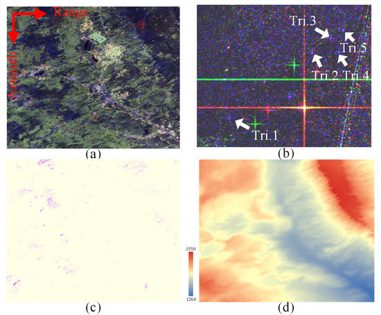
Figure 8. The Pauli-RGB images of study areas from GF-3 data. (a) The Pauli-RGB image of the calibration site in Inner Mongolia Province in China from GF-3 data. (b) The enlarged view of the red box in (a) with trihedral corner reflectors. (c) Selected Bragg-like targets area; (d) DEM image of the illuminating site.

Table 3. Quality evaluation of trihedral corner reflectors in the Mongolia calibration campaign for GF-3 Pol-SAR data.

	Tri.1	Tri.2	Tri.3	Tri.4	Tri.5
$\left|VV/HH\right|$	0.3520	0.3907	0.3431	0.1916	0.4534
$\angle VV/HH$	4.7436	7.5901	5.1934	4.0472	5.1239
$\left|HV/HH\right|$	−38.1759	−35.9219	−36.5847	−36.4814	−36.9791
$\left|VH/HH\right|$	−39.0578	−36.0557	−36.4357	−37.8592	−37.0913

The entire image was operated by using a 7 × 7 multilook operation to reduce the speckle noise before estimating the channel imbalances. The Bragg-like targets were selected by setting the correlation coefficients $R_{hhvv}$ to 0.9 and setting the ENL to 0.7. The size of each range bin was 100 so that the range pixels were divided into 80 bins. Since we verified that the different blocks in the azimuth direction had a significant influence on the estimated results and that the fusion block was more accurate in most cases, 100-, 64-, 32-, 16-, and 0-blocks were used to derive the final fusion results in the range direction. The LSL values corresponding to the range bins where the trihedral corner reflectors are located were averaged and used to calibrate the Sinclair matrices of the trihedral corner reflectors. The calibration results are shown in Table 4, and the crosstalk values were approximately identical to the corresponding values in Table 3 since the crosstalk was not estimated and calibrated. The copol channel imbalances of the trihedral corner reflectors were less than 0.3 dB and 5°, except for Tri.2. The phase of the copol channel imbalance of Tri.2 was evaluated as 7.5901° before calibration by the estimated results, which largely deviated from the ideal value. However, the copol channel imbalance was improved to 5.4749° by using the proposed algorithm. Table 4 shows that the copol channel imbalance amplitudes and phases were closer to the theoretical values of the trihedral corner reflectors after calibration when using the estimation values of our method.

Table 4. Quality evaluation of trihedral corner reflectors after calibrating by using the estimated channel imbalance.

	Tri.1	Tri.2	Tri.3	Tri.4	Tri.5
$\left|VV/HH\right|$	0.2013	0.2182	0.1561	0.0166	0.2725
$\angle VV/HH$	2.6912	5.4749	3.0451	2.1655	3.0288
$\left|HV/HH\right|$	−36.1654	−36.6482	−37.0742	−35.7543	−35.8580
$\left|VH/HH\right|$	−37.8945	−37.0951	−36.3498	−36.4834	−35.3586

To verify the reliability of the x-pol channel imbalance, we also utilized the Ainsworth, ZeroAinsworth, and Quegan [12,13] algorithms to estimate the x-pol channel imbalance $\alpha$ in (3), with three volume-scattering dominated and homogeneous areas selected artificially. Since the LSL values derived by the proposed method varied with the range direction and the gradient was very close to 0, the estimated x-pol channel imbalance was provided by an average filter operation, which is different from the AFO and PFO. First, the estimated transmitting and receiving channel imbalances of the fusion results were used to derive the x-pol channel imbalance using (6). Second, the candidate values were selected by using the histogram of the x-pol channel imbalance to ensure that at least 85% of the values were used for averaging. Finally, the x-pol channel imbalance of the entire image was obtained by averaging the candidates to compare it with the other calibration algorithms. The comparison results are shown in Table 5. The difference in amplitude between the proposed method and the other three methods was approximately 0.06 dB, and the deviation of phase between the four methods was less than 0.5°. Although Table 5 shows that the amplitude and the phase absolute value of $\alpha$ estimated by using the proposed method were higher, the result from the proposed method retained the consistency in amplitude and phase mentioned above when compared with other methods, validating the effectiveness of our method.

Table 5. Comparison of $\left|\alpha \right|$ (dB) and $Arg(\alpha )$ (°) provided by Ainsworth, ZeroAinsworth, Quegan, and the proposed method.

	Ainsworth	ZeroAinsworth	Quegan	the Proposed Method
$\left|\alpha \right|$	−0.4957	−0.4979	−0.5089	−0.4300
$Arg(\alpha )$	2.3456	2.3470	2.3455	2.7138

5. Discussion

5.1. Influence of Crosstalk

In recent Pol-SAR systems, the crosstalk was less than −20 dB [30], and so it is not the main calibrated parameter of concern in this paper. The accuracy of the estimated transmitting and receiving channel imbalance was influenced by crosstalk according to (2). It should be noted that crosstalk can influence the proposed method from two perspectives. First, the indicators of selecting Bragg-like targets, including $R_{hhvv}$ and ENL, are influenced by the crosstalk, so that the effectiveness of the selection is based on the assumption that the crosstalk system is better than −20 dB [17]. Second, some of the terms corresponding to crosstalk are negligible in (24) and (38), to simplify the derivation of our method when the crosstalk is small. To focus on the influence of crosstalk on the algorithm itself rather than the influence on the selection of Bragg-like targets, the desert area was selected as the study region. The crosstalk was added to the standard GF-3 QPSI mode product, whose amplitude of crosstalk varied from −25 dB to −15 dB. We set the amplitude of crosstalk as being identified for each simulated experiment, with random phases. The simulated channel imbalance values were the same as those in the simulation in Section 4. Table 5 shows that the 0-block in the azimuth direction has the least error for the desert dataset, and the following simulated experiment is based on the 0-block in the azimuth direction. The 0-block results of different crosstalk are shown in Figure 9.

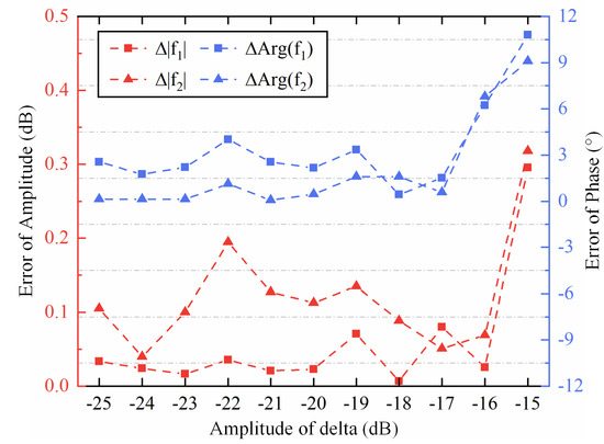
Figure 9. The fusion error of simulated GF-3 data, distorted by different $\delta$.

Figure 9 shows that the error of the estimated channel imbalances by using the proposed method was within 0.5 dB and 5° when the crosstalk was less than −17 dB, but the phase error reached over 6° and 10° when the crosstalk was −16 dB and −15 dB, respectively. The error was expected to monotonically increase as the amplitude of crosstalk increased. Nevertheless, fluctuation was occasionally apparent in the errors of both amplitude and phase in estimating the channel imbalances from Figure 9. Although the errors increased at first and then modestly decreased before climbing up again, the peak value of each increase was higher than the previous growth in most cases. The decrease was attributed to the best-fit solution, in which some false iterative results were excluded by the filter. Figure 10 and Figure 11 show the comparison of the estimation results, with −25 dB, −17 dB, −16 dB, and −15 dB crosstalk imposed.

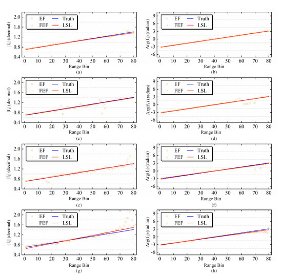
Figure 10. The estimated $f_1$ of the simulated GF-3 data. (a,c,e,g): The amplitude of the fusion-estimated $f_1$ after imposing −25 dB, −17 dB, −16 dB, and −15 dB crosstalk. (b,d,f,h): The phase of the fusion-estimated $f_1$ after imposing −25 dB, −17 dB, −16 dB, and −15 dB crosstalk.

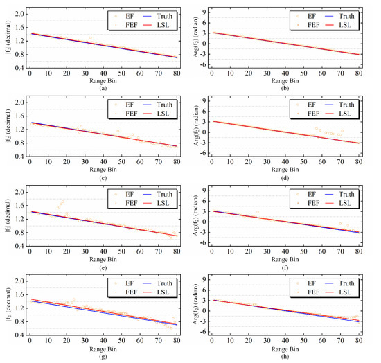
Figure 11. The estimated $f_2$ of simulated GF-3 data. (a,c,e,g): The amplitude of the fusion-estimated $f_2$ after imposing −25 dB, −17 dB, −16 dB, and −15 dB crosstalk. (b,d,f,h): The phase of the fusion-estimated $f_2$ after imposing −25 dB, −17 dB, −16 dB, and −15 dB crosstalk.

As shown in Figure 10 and Figure 11, the number of incorrect range bins in the image simulated by adding −15 dB crosstalk was more than those simulated by a −25 dB crosstalk, but the most inaccurate estimation results at different range bins were not selected to fit the final LSL when the added crosstalk is high, leading to the relatively small error in amplitude. Phase ambiguity elimination still existed in some range bins when the crosstalk became higher, which was caused by the failure to eliminate the ambiguity of ${\phi }_{-}$. When the crosstalk was more than −20 dB and the inaccuracy of selecting Bragg-like targets increased, the term corresponding to crosstalk in (36) cannot be ignored, so that the phase of $O_{23}$ cannot eliminate the ambiguity of ${\phi }_{-}$. However, due to the filter operation, those ambiguous phases were not included in the final results and they do not influence the precision of the estimation.

The crosstalk level limits both the accuracy of selecting Bragg-like targets and the negligible parts in (24) and (38) during our deviation. It has been proven that the selection of Bragg-like targets is faithful when the crosstalk of uncalibrated polarimetric images is lower than −20 dB. Additionally, the simulated experiment mentioned above verified that ignoring crosstalk in the part of the deviation did not have a significant influence on the accuracy of estimations after the filter and fitting operation when it was lower than −17 dB. In summary, the influence of crosstalk on the applicability of the proposed method can be ignored when the crosstalk of the Pol-SAR system is under −20 dB.

5.2. Influence of Noise

Additive noise may significantly bias the estimation when HV and VH scattering from Bragg-like targets is low, which is why vegetation pixels are believed to be better candidates to solve the x-pol imbalance and crosstalk, because of their strong x-pol signal return in the existing method. In this section, the influence of noise on the x-pol channel imbalance estimation is analyzed, with a comparison between the proposed method and the Ainsworth method. The estimation of the x-pol channel imbalance in our method is based on the coherence components of x-pol and copol ($C_{mn}(m=1,4,n=2,3)$) in the covariance matrix, while the estimation relies on the x-pol components ($C_{nn}(n=2,3)$) in the Ainsworth algorithm. In general, the additive noise is decoherence in the channel, which is mentioned in [38]. Therefore, under the condition that Bragg-like targets are used as candidate points, additive noise has less influence on the proposed method. In the following, the influence of additive noise on the estimation of x-pol channel imbalance is analyzed by the desert dataset, with both channel imbalances and additive noise added.

It should be noted that there generally exists original noise in the actual Pol-SAR image. Therefore, the original noise level should be considered as the a priori knowledge when assessing the noise floor after adding the extra noise. The noise equivalent sigma zero (NESZ) is considered as an indicator of additive noise in an SAR image. However, the header files of the Gaofen-3 product did not provide NESZ, so Shi estimated the NESZ values of Gaofen-3 QPSI images and provided the results with a table that presented NESZ values in different beam codes. The header file of the dataset in this section shows that the beam code is 199, whose NESZ ranges from −39.9 dB to −34.9 dB according to Table III in [38]. Therefore, the original noise is considered to be −37.5 dB in the desert dataset. Based on this, we impose the extra noise to the image for analysis.

Before adding the noise into the original image, the x-pol channel imbalance with an amplitude of −3 dB to 3 dB and a phase of $-\pi$ to $\pi$, and the copol channel imbalance with an amplitude of 3 dB to −3 dB and a phase of $\pi$ to $-\pi$ are imposed into the Pol-SAR data. Then, the noise is added to the Pol-SAR image according to (1). The intensity extent of the added noise is from −35 dB to −25 dB, and the phase is randomly picked from $-\pi$ to $\pi$. The candidate Bragg-like pixels were input into both the Ainsworth method and the proposed method.

In Figure 12, amplitude and phase errors brought about by the proposed method and the Ainsworth method are represented when the intensity of the added noise is −35 dB, −30 dB, and −25 dB. The estimated results in each range direction, which are represented by the red balls and green asterisks in Figure 12, show that although the cross-polarization channel imbalance added to the image changes linearly along the range direction, it was no longer appropriate to fit the amplitude of estimation with the linear fitting since the estimated values along the range patch were not linear, apparently. Therefore, the second-order curve fitting was performed on the amplitude estimated value, and the linear fitting was still used for the phase estimated value. The fitting curves are represented by red and green lines. The estimated phase results by both two methods were close to the truth values. As for amplitude, Figure 12 shows that the red curves were closer to the truth than the green ones, which means that the error caused by the proposed method was smaller. The Ainsworth method is more sensitive to noise when Bragg-like pixels are input into the algorithm since only adding −35 dB noise can result in a significant bias away from the truth. However, as demonstrated by the estimated results in each range direction, the stability of the proposed algorithm was lower than that of the Ainsworth algorithm, but it was enhanced as the added noise decreased.

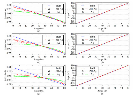
Figure 12. X-pol channel imbalance estimation results by using the proposed method (ZH-Ag) and the Ainsworth (Ag) algorithm. (a,c,e): The amplitude of estimated $\alpha$ under the case that the amplitude of added noise is −35 dB, −30 dB, and −25 dB, respectively; (b,d,f): The phase of estimated $\alpha$ under the case that the amplitudes of added noise is −35 dB, −30 dB, and −25 dB, respectively.

6. Conclusions

In this paper, we proposed a method for estimating transmitting and receiving channel imbalances based on the zero helix property of Bragg-like pixels. After obtaining the estimated values of the channel imbalances from the UZHEX constraint and reciprocity assumption by using the automatically selected Bragg-like targets, the phase ambiguity is eliminated by using the reciprocity and the first element of the normalized mean coherence matrix $⟨N_{11}⟩$ based on the $H/\overline{\alpha }$ decomposition. The final estimated channel imbalances are derived after the filter and fitting operation, for more reliable results. Both the simulated data from the ALOS and GF-3 Pol-SAR datasets with different types of land cover in the scenes and real data from the GF-3 calibration campaigns with several corner reflectors on site were used to test our method. According to the simulated results, the proposed method exhibited a stable performance in most scenes, with enough Bragg-like targets. In general, the error of our method can be within 0.5 dB for amplitude and 5° for phase from the simulated data. In terms of the real data, both the copol and x-pol channel imbalances were improved after calibration by using the estimated values. The amplitude of the $VV/\phantom{VVHH}HH$ term of the trihedral corner reflectors was less than 0.3 dB, and the phase was less than 5.5°. The results from simulating Pol-SAR data by imposing crosstalk on the desert data indicated that the method exhibited stable performance when the crosstalk was larger than −20 dB if the selection of pixels was sufficiently accurate. Compared with the Ainsworth algorithm, the proposed method yielded more accurate estimation results when the SNR of the image was decreasing. By simulating the noise added to the desert data, we demonstrated that the error caused by our method was within 0.5 dB, and 3° when the added noise was under −27 dB for the dessert data that we used in the paper.

Since the crosstalk can be roughly estimated in the proposed method, in future work, we will focus on the accurate estimation of the crosstalk by using bare soil. Given that the estimated precision of channel imbalances is influenced by both the number and the accuracy of selecting candidates for the UZHEX constraint, accurately extracting a large number of Bragg-like targets is another topic for future research. In addition, in order to apply our algorithm to all the spaceborne system, the influence caused by the Faraday rotation angle should be considered and eliminated in future work.

References

- Zebker, H.A.; Van Zyl, J.J. Imaging radar polarimetry: A review. Proc. IEEE 1991, 79, 1583–1606. [Google Scholar] [CrossRef]
- Qi, Z.; Yeh, A.G.O.; Li, X.; Zhang, X. A three-component method for timely detection of land cover changes using polarimetric SAR images. ISPRS J. Photogramm. Remote Sens. 2015, 107, 3–21. [Google Scholar] [CrossRef]
- Varade, D.; Manickam, S.; Dikshit, O.; Singh, G.; Snehmani. Modelling of early winter snow density using fully polarimetric C-band SAR data in the Indian Himalayas. Remote Sens. Environ. 2020, 240, 111699. [Google Scholar] [CrossRef]
- Shokr, M.; Dabboor, M. Observations of SAR polarimetric parameters of lake and fast sea ice during the early growth phase. Remote Sens. Environ. 2020, 247, 111910. [Google Scholar] [CrossRef]
- Chang, Q.; Zwieback, S.; DeVries, B.; Berg, A. Application of L-band SAR for mapping tundra shrub biomass, leaf area index, and rainfall interception. Remote Sens. Environ. 2022, 268, 112747. [Google Scholar] [CrossRef]
- Shi, H.; Zhao, L.; Yang, J.; Lopez-Sanchez, J.M.; Zhao, J.; Sun, W.; Shi, L.; Li, P. Soil moisture retrieval over agricultural fields from L-band multi-incidence and multitemporal PolSAR observations using polarimetric decomposition techniques. Remote Sens. Environ. 2021, 261, 112485. [Google Scholar] [CrossRef]
- Komarov, A.S.; Zabeline, V.; Barber, D.G. Ocean surface wind speed retrieval from C-band SAR images without wind direction input. IEEE Trans. Geosci. Remote Sens. 2013, 52, 980–990. [Google Scholar] [CrossRef]
- Freeman, A. SAR calibration: An overview. IEEE Trans. Geosci. Remote Sens. 1992, 30, 1107–1121. [Google Scholar] [CrossRef]
- Whitt, M.; Ulaby, F.; Polatin, P.; Liepa, V. A general polarimetric radar calibration technique. IEEE Trans. Antennas Propag. 1991, 39, 62–67. [Google Scholar] [CrossRef]
- Zhu, L.; Walker, J.P.; Ye, N.; Rüdiger, C.; Hacker, J.M.; Panciera, R.; Tanase, M.A.; Wu, X.; Gray, D.A.; Stacy, N.; et al. The polarimetric L-band imaging synthetic aperture radar (PLIS): Description, calibration, and cross-validation. IEEE J. Sel. Top. Appl. Earth Obs. Remote Sens. 2018, 11, 4513–4525. [Google Scholar] [CrossRef]
- Li, L.; Zhu, Y.; Hong, J.; Ming, F.; Wang, Y. Design and implementation of a novel polarimetric active radar calibrator for Gaofen-3 SAR. Sensors 2018, 18, 2620. [Google Scholar] [CrossRef] [PubMed]
- Quegan, S. A unified algorithm for phase and cross-talk calibration of polarimetric data-theory and observations. IEEE Trans. Geosci. Remote Sens. 1994, 32, 89–99. [Google Scholar] [CrossRef]
- Ainsworth, T.L.; Ferro-Famil, L.; Lee, J.S. Orientation angle preserving a posteriori polarimetric SAR calibration. IEEE Trans. Geosci. Remote Sens. 2006, 44, 994–1003. [Google Scholar] [CrossRef]
- Shimada, M. Model-based polarimetric SAR calibration method using forest and surface-scattering targets. IEEE Trans. Geosci. Remote Sens. 2011, 49, 1712–1733. [Google Scholar] [CrossRef]
- Freeman, A.; Durden, S.L. A three-component scattering model for polarimetric SAR data. IEEE Trans. Geosci. Remote Sens. 1998, 36, 963–973. [Google Scholar] [CrossRef]
- Shi, L.; Yang, J.; Li, P. Co-polarization channel imbalance determination by the use of bare soil. ISPRS J. Photogramm. Remote Sens. 2014, 95, 53–67. [Google Scholar] [CrossRef]
- Shi, L.; Li, P.; Yang, J.; Zhang, L.; Ding, X.; Zhao, L. Polarimetric SAR calibration and residual error estimation when corner reflectors are unavailable. IEEE Trans. Geosci. Remote Sens. 2020, 58, 4454–4471. [Google Scholar] [CrossRef]
- Shi, L.; Li, P.; Yang, J.; Sun, H.; Zhao, L.; Zhang, L. Polarimetric calibration for the distributed Gaofen-3 product by an improved unitary zero helix framework. ISPRS J. Photogramm. Remote Sens. 2020, 160, 229–243. [Google Scholar] [CrossRef]
- Shangguan, S.; Qiu, X.; Fu, K.; Lei, B.; Hong, W. GF-3 Polarimetric Data Quality Assessment Based on Automatic Extraction of Distributed Targets. IEEE J. Sel. Top. Appl. Earth Obs. Remote Sens. 2020, 13, 4282–4294. [Google Scholar] [CrossRef]
- Azcueta, M.; D’Alessandro, M.M.; Zajc, T.; Grunfeld, N.; Thibeault, M. ALOS-2 preliminary calibration assessment. In Proceedings of the IGARSS 2015—2015 IEEE International Geoscience and Remote Sensing Symposium, Milan, Italy, 26–31 July 2015. [Google Scholar]
- Touzi, R.; Hawkins, R.K.; Cote, S. High Precision Assessment and Calibration of Polarimetric RADARSAT-2 Using Transponder Measurements. In Proceedings of the PolinSAR 2011, Science and Applications of SAR Polarimetry and Polarimetric Interferometry, Frascati, Italy, 24–28 January 2011; Volume 695. [Google Scholar]
- Zhao, X.; Deng, Y.; Zhang, H.; Liu, X. A Channel Imbalance Calibration Scheme with Distributed Targets for Circular Quad-Polarization SAR with Reciprocal Crosstalk. Remote Sens. 2023, 15, 1365. [Google Scholar] [CrossRef]
- Praks, J.; Hallikainen, M. A novel approach in polarimetric covariance matrix eigendecomposition. In Proceedings of the IGARSS 2000, IEEE 2000 International Geoscience and Remote Sensing Symposium. Taking the Pulse of the Planet: The Role of Remote Sensing in Managing the Environment. Proceedings (Cat. No. 00CH37120), Honolulu, HI, USA, 24–28 July 2000; IEEE: Piscataway, NJ, USA, 2000; Volume 3, pp. 1119–1121. [Google Scholar]
- Cloude, S.R.; Pottier, E. A review of target decomposition theorems in radar polarimetry. IEEE Trans. Geosci. Remote Sens. 1996, 34, 498–518. [Google Scholar] [CrossRef]
- Cloude, S.; Pottier, E. An entropy based classification scheme for land applications of polarimetric SAR. IEEE Trans. Geosci. Remote Sens. 1997, 35, 68–78. [Google Scholar] [CrossRef]
- Cloude, S.R.; Ossikovski, R.; Garcia-Caurel, E. Bright singularities: Polarimetric calibration of spaceborne PolSAR systems. IEEE Geosci. Remote Sens. Lett. 2020, 18, 476–479. [Google Scholar] [CrossRef]
- Van Zyl, J.J. Calibration of polarimetric radar images using only image parameters and trihedral corner reflector responses. IEEE Trans. Geosci. Remote Sens. 1990, 28, 337–348. [Google Scholar] [CrossRef]
- Yamaguchi, Y.; Moriyama, T.; Ishido, M.; Yamada, H. Four-component scattering model for polarimetric SAR image decomposition. IEEE Trans. Geosci. Remote Sens. 2005, 43, 1699–1706. [Google Scholar] [CrossRef]
- Nghiem, S.; Yueh, S.; Kwok, R.; Li, F. Symmetry properties in polarimetric remote sensing. Radio Sci. 1992, 27, 693–711. [Google Scholar] [CrossRef]
- Chang, Y.; Zhao, L.; Shi, L.; Nie, Y.; Hui, Z.; Xiong, Q.; Li, P. Polarimetric calibration of SAR images using reflection symmetric targets with low helix scattering. Int. J. Appl. Earth Obs. Geoinf. 2021, 104, 102559. [Google Scholar] [CrossRef]
- Fore, A.G.; Chapman, B.D.; Hawkins, B.P.; Hensley, S.; Jones, C.E.; Michel, T.R.; Muellerschoen, R.J. UAVSAR polarimetric calibration. IEEE Trans. Geosci. Remote Sens. 2015, 53, 3481–3491. [Google Scholar] [CrossRef]
- Praks, J.; Koeniguer, E.C.; Hallikainen, M.T. Alternatives to target entropy and alpha angle in SAR polarimetry. IEEE Trans. Geosci. Remote Sens. 2009, 47, 2262–2274. [Google Scholar] [CrossRef]
- Rabus, B.; Eineder, M.; Roth, A.; Bamler, R. The shuttle radar topography mission—A new class of digital elevation models acquired by spaceborne radar. ISPRS J. Photogramm. Remote Sens. 2003, 57, 241–262. [Google Scholar] [CrossRef]
- Lee, J.S.; Schuler, D.L.; Ainsworth, T.L. Polarimetric SAR data compensation for terrain azimuth slope variation. IEEE Trans. Geosci. Remote Sens. 2000, 38, 2153–2163. [Google Scholar]
- Borner, T.; Papathanassiou, K.P.; Marquart, N.; Zink, M.; Meadows, P.; Rye, A.; Wright, P.; Meininger, M.; Tell, B.R.; Traver, I.N. ALOS PALSAR products verification. In Proceedings of the 2007 IEEE International Geoscience and Remote Sensing Symposium, Barcelona, Spain, 23–27 July 2007; IEEE: Piscataway, NJ, USA, 2007; pp. 5214–5217. [Google Scholar]
- Shimada, M.; Isoguchi, O.; Tadono, T.; Higuchi, R.; Isono, K. PALSAR CALVAL summary and update 2007. In Proceedings of the 2007 IEEE International Geoscience and Remote Sensing Symposium, Barcelona, Spain, 23–27 July 2007; IEEE: Piscataway, NJ, USA, 2007; pp. 3593–3596. [Google Scholar]
- Zhang, Q. System design and key technologies of the GF-3 satellite. Acta Geod. Cartogr. Sin. 2017, 46, 269–277. [Google Scholar]
- Shi, L.; Yang, L.; Zhao, L.; Li, P.; Yang, J.; Zhang, L. NESZ Estimation and Calibration for Gaofen-3 Polarimetric Products by the Minimum Noise Envelope Estimator. IEEE Trans. Geosci. Remote Sens. 2021, 59, 7517–7534. [Google Scholar] [CrossRef]
Disclaimer/Publisher’s Note: The statements, opinions and data contained in all publications are solely those of the individual author(s) and contributor(s) and not of MDPI and/or the editor(s). MDPI and/or the editor(s) disclaim responsibility for any injury to people or property resulting from any ideas, methods, instructions or products referred to in the content. |
© 2023 by the authors. Licensee MDPI, Basel, Switzerland. This article is an open access article distributed under the terms and conditions of the Creative Commons Attribution (CC BY) license (https://creativecommons.org/licenses/by/4.0/).