Article

P2FEViT: Plug-and-Play CNN Feature Embedded Hybrid Vision Transformer for Remote Sensing Image Classification

1
School of Information and Electronics, Beijing Institute of Technology, Beijing 100081, China
2
Beijing Key Laboratory of Embedded Real-Time Information Processing Technology, Beijing 100081, China
3
School of Computer Science, Peking University, Beijing 100871, China
4
Shanghai AI Laboratory, Shanghai 200232, China
*
Author to whom correspondence should be addressed.
Remote Sens. 2023, 15(7), 1773; https://doi.org/10.3390/rs15071773
Submission received: 2 March 2023 / Revised: 22 March 2023 / Accepted: 23 March 2023 / Published: 26 March 2023
(This article belongs to the Special Issue Remote Sensing Image Processing with Transformers)

Abstract

:
Remote sensing image classification (RSIC) is a classical and fundamental task in the intelligent interpretation of remote sensing imagery, which can provide unique labeling information for each acquired remote sensing image. Thanks to the potent global context information extraction ability of the multi-head self-attention (MSA) mechanism, visual transformer (ViT)-based architectures have shown excellent capability in natural scene image classification. However, in order to achieve powerful RSIC performance, it is insufficient to capture global spatial information alone. Specifically, for fine-grained target recognition tasks with high inter-class similarity, discriminative and effective local feature representations are key to correct classification. In addition, due to the lack of inductive biases, the powerful global spatial context representation capability of ViT requires lengthy training procedures and large-scale pre-training data volume. To solve the above problems, a hybrid architecture of convolution neural network (CNN) and ViT is proposed to improve the RSIC ability, called P 2 FEViT, which integrates plug-and-play CNN features with ViT. In this paper, the feature representation capabilities of CNN and ViT applying for RSIC are first analyzed. Second, aiming to integrate the advantages of CNN and ViT, a novel approach embedding CNN features into the ViT architecture is proposed, which can make the model synchronously capture and fuse global context and local multimodal information to further improve the classification capability of ViT. Third, based on the hybrid structure, only a simple cross-entropy loss is employed for model training. The model can also have rapid and comfortable convergence with relatively less training data than the original ViT. Finally, extensive experiments are conducted on the public and challenging remote sensing scene classification dataset of NWPU-RESISC45 (NWPU-R45) and the self-built fine-grained target classification dataset called BIT-AFGR50. The experimental results demonstrate that the proposed P 2 FEViT can effectively improve the feature description capability and obtain outstanding image classification performance, while significantly reducing the high dependence of ViT on large-scale pre-training data volume and accelerating the convergence speed. The code and self-built dataset will be released at our webpages.

1. Introduction

As the fundamental task in remote sensing image interpretation, image classification has critical applications in many fields, such as intelligent transportation, precision agriculture, urban planning, military monitoring, etc. [1,2,3,4,5]. In recent years, there has been a proliferation of image classification algorithms that continue to set new performance records in natural scene datasets, such as ImageNet [6], CIFAR [7], Fashion-MNIST [8], etc. At the algorithm level, they can be divided into two categories according to the feature extractor. The first category is convolutional neural network (CNN)-based methods; as the basis of modern deep learning technology, classical CNN-based image classification algorithms have continuously achieved performance breakthroughs within the last decade. In the early period, classification networks, such as LeNet5 [9], AlexNet [10], VGG [11], GoogleNet [12], and other simple shallow convolutional neural networks, relying on the CNN’s ability to extract image features, far exceeded other traditional machine learning algorithms [13,14,15] in classification performance. Next, with the emergence of ResNet [16] residual networks, CNN-based image classification networks gradually developed into deeper layers. The better feature description ability acquired by continuously deepening the network and constructing better inter-layer connections further improved the network generalization ability and classification performance. In recent years, CNN-based image classification networks, such as NFNet [17], ConvNext [18], ResNest [19], etc., have still shown excellent performance in natural scene image classification through their specifically designed network structure.
The second category is vision transformer (ViT)-based methods [20,21,22,23]. Just as CNNs have dominated visual representation in the last decade, the Transformer has the same status in the field of natural language processing (NLP). In the early period of computer vision, the Transformer was used as a feature aggregator in object detection or video understanding to extract global context information from images. However, its performance was not remarkable, so it has been neglected for several years. In the last two years, excellent CNN-free Transformer classification networks, such as ViT and SWIN-Transformer [20,21], have emerged and broken the domination of CNN on natural scene benchmarks, such as ImageNet [6] and CIFAR [7]. After researchers realized the excellent performance of ViT in the field of computer vision, CNN-free classification networks based on ViT and SWIN-Transformer emerged one after another.
Unlike natural scene images, remote sensing images often have large scale and tonal differences between the same class of objects due to different image acquisition conditions. In addition, the objects in remote sensing scene images often present significant inter-class similarity and intra-class differences, as shown in Figure 1. Figure 1a presents different examples of the same categories. It can be intuitively seen that the intra-class variance is large in remote sensing images. Figure 1b shows instance samples of different categories, which are easily confused because of the significant inter-class similarities. In remote sensing image classification (RSIC) tasks, better global context information representation is essential to improve classification performance, while stronger local feature description facilitates the network to better identify remote sensing targets with slight inter-class variability, both of which are indispensable. These objective factors make it necessary for the network to have better feature representation capability with the aim of achieving satisfactory performance in the field of RSIC. Moreover, with the development of modern optical remote sensing technology, the volume of available remote sensing images has been increasing rapidly. However, the available labeled training data volume is still much less than that for natural scenes. Therefore, RSIC is a demanding and challenging research topic.
As analyzed above, the research on RSIC has recently mainly focused on improving the feature description capability of the network. To obtain better global context information and local feature representations, researchers have tried to integrate global information into the CNN structure through various methods [25,26,27,28,29,30]. For example, Cheng et al. [25] specifically designed a stacking CNN architecture based on the ensemble learning method. First, a modified multi-scale CNN is applied to capture multi-scale structural features. Then, a hidden Markov model (HMM) is utilized to gather global information on the structural features. The final prediction is generalized through ensemble learning of extreme gradient boosting (XGBoost). Wang et al. [26] constructed a deformable CNN structure to make the sampling positions adapt to the shape of targets in the remote sensing images; the spatial-channel attention mechanisms are used to obtain a better global feature description. A parallel CNN-based self-adaptive attention network is proposed in [27]. First, a parallel convolutional block is applied to capture multiscale fused features. Then, a sequential convolutional attention block is designed to obtain global context features. The global context features are classified through a series of residual blocks with the attention mechanism and a fully connected (FC) layer. However, the limited effective receptive field (ERF) of CNN restricts the performance of image classification networks. The value of each unit in a convolutional network depends only on a region of the input, which is the so-called receptive field. The size of the receptive field is a key issue in CNN-based image classification methods because the output must respond to a sufficiently large region of the image to capture enough context information for image classification or target recognition. Once the receptive field is insufficient, the network will only focus on a limited region which cannot represent the feature of the whole object. The receptive field can be linearly increased by staking more layers or multiplicatively increased through pooling operations. However, in the receptive field study for CNNs, [31] states that not all pixels in CNNs contribute equally to the receptive field. Pixels in the central part have a larger impact on the output receptive field. In addition, the ERF of CNNs tends to be smaller than the theoretical receptive field (TRF). This indicates that CNNs are more concerned with local feature representation and are limited in their ability to extract global context information. In addition, [32] points out that the ERF of traditional CNNs with stacking deep layers of small convolution kernels, such as ResNet101 [16] and ResNet152 [16], is actually not large, proving that the method of deepening the network by convolution and pooling cannot obtain a larger ERF. For remote sensing images with complex scenes and significant target scale variations, the restriction of ERF in CNN makes it challenging to obtain global context information, which essentially limits its feature representation capability. Therefore, although the above-mentioned researchers have tried introducing global context information in different ways to enhance the feature representation capability of CNNs, the existing methods still have room for enhancement due to the constrained ERF of CNNs. With the proposal of ViT in computer vision, thanks to Transformer’s self-attention mechanism, it can effectively capture global context information. The multi-head self-attention mechanism (MSA) can map long-range relationships to multiple spaces for more potent global contextual information representation. For example, Bazi et al. [33] directly applied the ViT model to solve image classification in remote sensing images and proposed a series of data augmentation strategies to expand the training data volume for ViT’s training procedure. To fuse the channel attention to the ViT, Lv et al. [34] proposed a spatial-channel feature-preserving ViT model, which considers both the global context information of the image and the contribution of the different channels in the classification token. However, since ViT only considers the relationship between patches and ignores the information inside them, it cannot effectively model the local features, which is non-negligible for RSIC. In addition, due to the lack of inductive bias in the Transformer, the ViT models generally depend on a very large scale pre-training data volume to obtain better performance. In summary, existing works on feature representation improvement are mainly concentrated in CNN or ViT, each of which has its own advantages and shortcomings. For example, CNN can capture local discriminative features quickly and effectively, but cannot capture global spatial context information effectively. ViT can capture global spatial context information through lengthy and large data training but ignores local discriminative information in local patch tokens. Therefore, an effective feature representation approach that can combine local discriminative features and global spatial context information needs to be further explored to improve the performance of RSIC.
To address the limitations of existing methods in terms of feature representation, a plug-and-play CNN feature embedded hybrid vision transformer, so-called P 2 FEViT, is proposed in this paper, which fully combines the advantages of CNN and ViT without complex specific network design. The proposed hybrid network allows embedding features extracted from any CNN structure as a plug-and-play module into the ViT architecture. The flexibility allows us to easily combine different CNN features with ViT structures and, thus, create a hybrid ViT network. In addition, the plug-and-play feature provides more experimental flexibility, thus helping to explore potential combinations of various CNN features with ViT architectures for better RSIC performance. The fusion of ViT and CNN by feature embedding makes full use of the local feature description capability of CNN and the representation ability of ViT for global context information. Through complementation, the convergence speed and generalization ability of ViT can be improved significantly. Since inductive biases can be attached by the embedding CNN features, the hybrid network can reduce the reliance of ViT on a very large-scale pre-training data volume to achieve better classification performance. In this paper, we first intuitively analyze the feature representation capabilities of CNN and ViT models. Then, the detailed structure of the proposed P 2 FEViT is elaborated. Third, based on the hybrid structure, only a simple cross-entropy loss is employed for model training, and the model can achieve state-of-the-art (SOTA) classification performance as well as faster convergence than the original ViT. Furthermore, we collect remote sensing images containing aircraft targets of various scales and categories from Google Earth and construct an aircraft fine-grained recognition dataset, BIT-AFGR50. To verify the effectiveness of the proposed method, we conducted extensive experiments on the publicly available remote sensing scene classification dataset, NWPU-RESISC45 (NWPU-R45) [24], and the self-built BIT-AFGR50. The contributions can be summarized below:
(1)
A new hybrid classification architecture according to CNN and ViT is proposed for RSIC, which can be applied to complicated remote sensing scene classification and fine-grained target recognition tasks.
(2)
To address the limitations of existing methods in terms of feature representation, a novel approach embedding plug-and-play CNN features to ViT model is proposed, which can make full use of the local feature description capability of CNN and the representation ability of ViT for global context information to achieve better classification performance, as well as to reduce the high dependence of ViT models on large-scale pre-training data volume.
(3)
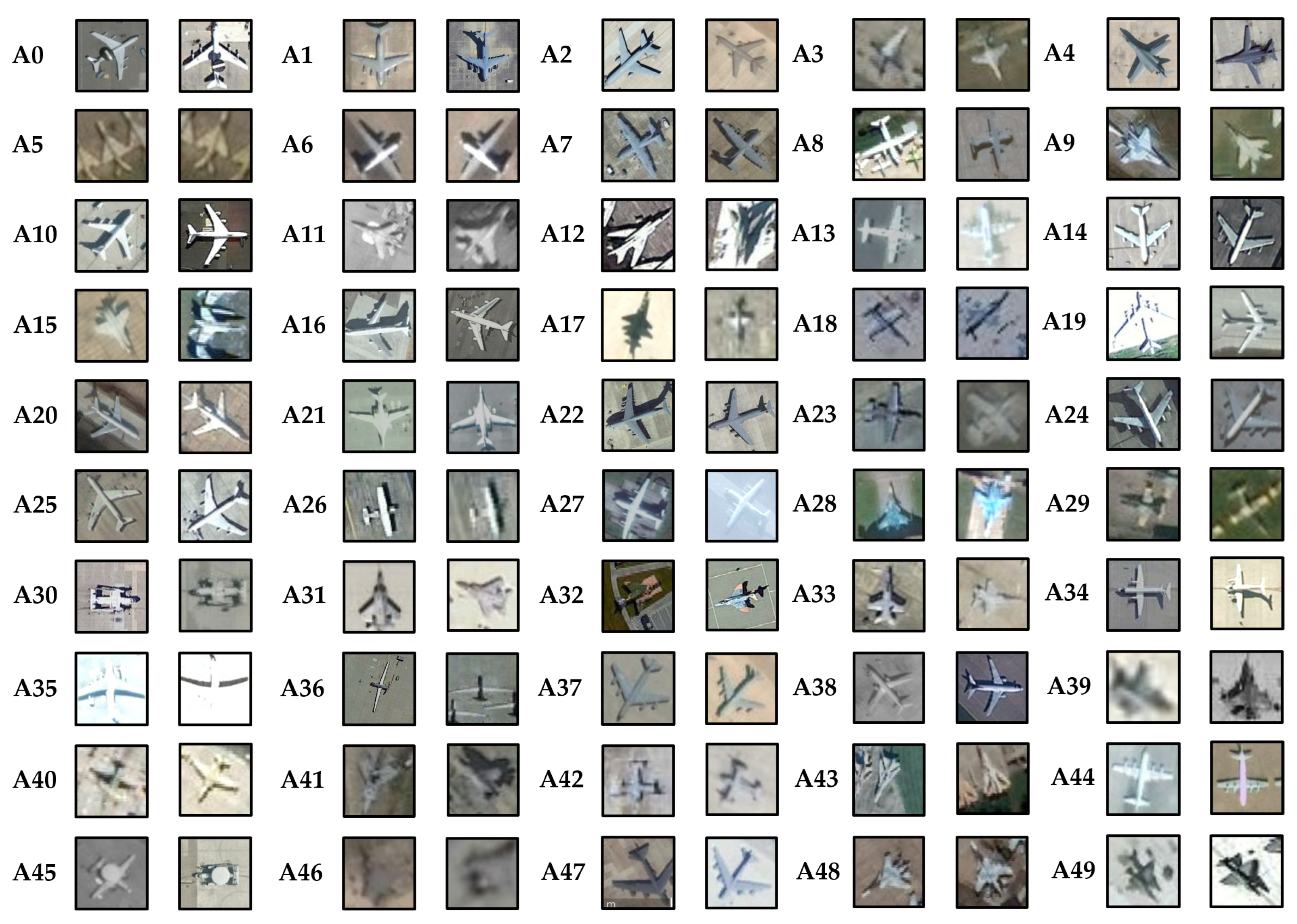
Considering that a large number of datasets are constructed based on the remote sensing scene classification task and relatively few datasets for the fine-grained target recognition task, a new fine-grained target recognition dataset is constructed in this paper, which contains 50 categories of aircraft targets aiming to facilitate scholars to carry out research on fine-grained target recognition.

2. Related Work

2.1. Review of Remote Sensing Image Classification Methods

With the increase in spatial resolution of remote sensing images, RSIC tasks are generally refined into three types: pixel-level classification, also known as semantic segmentation, target-level classification, and scene-level classification. In this paper, we refer to these three types of tasks collectively as RSIC. Driven by realistic task requirements, RSIC has been a hot research topic for researchers in recent decades, and many excellent RSIC algorithms have been proposed. Thanks to the development of modern optical remote sensing technology, much more remote sensing image data can be obtained, and data-driven deep learning-based algorithms are gradually being recognized. As the winner of the 2012 ImageNet image classification challenge, a convolutional neural network (CNN)-based image classification algorithm AlexNet [10] set off a boom in research on CNN-based algorithms. Around 2015, research on CNN-based RSIC algorithms gradually made progress. Penatti et al. [35] introduced CNNs in RSIC algorithms and evaluated the generalization capability of deep features, which achieved the most SOTA performance on the well-known remote sensing public dataset UC Merced [36]. It was shown that CNN can acquire higher-level image features than traditional hand-crafted feature-based methods [37,38,39], and is superior in generalization and robustness. In recent years, there have been numerous studies on CNN-based RSIC algorithms. To improve the classification performance, researchers have mainly focused on the following aspects, which can be summarized as feature-level, data-level, and strategy-level. First, in order to obtain a better image feature representation capability for the network and, thus, improve the classification performance, numerous feature-level studies have been conducted [40,41,42]. For example, to improve the feature representation and generalization ability of CNN for detailed texture features, Song et al. [40] proposed an attention mechanism added to the CNN structure to eliminate the redundancy in CNN features, and wavelet transform was used to extract and reconstruct the feature map, which effectively improved the performance of RSIC. The study [41] designed a multi-scale attention (MSA) module to highlight the salient features and obtain the global contextual information representation. Shi et al. [42] proposed a multi-branch feature fusion network to improve the feature representation capability with multi-convolution cooperation.
Second, to enhance the classification performance with the limited labeled remote sensing image data volume, researchers have proposed a series of data-level studies [43,44,45,46,47,48]. For example, to improve the classification performance under long-tail distributed data, Miao et al. [43] proposed a class-imbalanced pseudo-label selection approach to evaluate the quality of unlabeled samples, which could effectively increase the available training data volume. To combat the lack of labeled training data, the study [44] presented a data augmentation method based on a spectral-indexed generative adversarial network (GAN). The spectral characteristic of images was applied to data augmentation through the spectral-indexed GAN. Zhang et al. [48] proposed an improved simple linear iterative cluster (SLIC)-based classification method, which can increase the effectiveness of pseudo-labeled samples. Stivaktakis et al. [45] proposed a dynamic data augmentation strategy to expand the training data volume in each batch by an online linear transformation. Xiao et al. [46] proposed a remote sensing image data augmentation approach based on a neural style transfer (NST). The transferred images are applied to increase the training data volume. In order to increase the data volume for arbitrary remote sensing datasets, Yu et al. [47] proposed a data augmentation approach by applying linear transformations to generate simulation data for constructing an augmented dataset, and the constructed dataset can be used to train models with better representation capability.
Since the loss function guides the whole training procedure, proper selection of the loss function plays a crucial role in deep-learning-based image classification methods. For strategy-level improvement, researchers have proposed a series of studies on the loss function [49,50,51,52,53]. The authors of [49] analyzed and compared different deep learning loss functions in RSIC tasks and proposed a loss function selection scheme. To combat the effect of the vanishing gradient problem in deeper CNNs, Bazi et al. [50] proposed a simple yet efficient auxiliary loss function to help CNNs to converge. To improve the classification performance without changing the network structure in the inference procedure, Zhang et al. [51] trained the network with multi-size images and applied triplet loss to introduce more supervision information. To achieve better classification performance under the restriction of limited, clearly labeled remote sensing images, Zhang et al. [52] improved the center loss to a semi-supervised form and designed a cooperative dual-branch architecture to integrate the labeled and unlabeled samples. Wei et al. [53] presented a marginal center loss with an adaptive margin to overcome the limitation of significant intra-class variations in RSIC tasks. The marginal center loss can separate hard samples and enhance the contributions of hard samples to minimize the variations in features of intra-class targets.
In 2020s, the Google team applied Transformer to the image classification task and proposed the ViT structure, which has demonstrated its excellent classification ability on ImageNet. Because of the simple and outstanding structure of ViT and its potent scalability, it has triggered subsequent related research [33,54,55,56]. Bazi et al. [33] directly applied the ViT model to the RSIC task. Unlike CNN, the ViT model can obtain long-range global context information among image patches through the self-attention mechanism. The powerful feature extraction capability allows ViT to present outstanding performance in RSIC tasks. Since then, improved ViT models have emerged in the field of RSIC. For example, to handle the scale variation and arbitrary orientations of targets in remote sensing images, Wang et al. [54] introduced a learnable rotation mechanism into the ViT to learn multi-scale windows with different orientation angles for attention calculation. To enhance the local features, Sha et al. [55] proposed a multi-instance ViT, which mainly depends on multiple-instance learning (MIL). The framework highlights the feature response of key local regions for RSIC. Deng et al. [56] proposed a hybrid CNN and ViT architecture to further boost the classification ability at the decision level. The model contains two independent branches which are constructed with CNN and ViT. Images are fed into the parallel branches independently, and a joint loss function is developed to optimize the classifier. To achieve better feature representation capability, several specific-designed CNN-ViT hybrid networks, such as container [57] and CoAtNet [58], have been studied in natural scene image classification. In this paper, we propose a hybrid CNN-ViT structure focused on feature-level improvement for RSIC. The goal of our method is to fully combine the advantages of CNN and ViT in feature representation, as well as to avoid a complex specific network design.

2.2. Remote Sensing Image Classification Benchmarks

Datasets play a crucial role in the development of RSIC algorithms. As optical remote sensing technology develops, the volume of remote sensing images has grown significantly, which makes it possible to construct large-scale RSIC datasets. In the past decade, many remote sensing scene image classification datasets have been constructed and made public by researchers to facilitate the study of RSIC algorithms. In 2010, Yang et al. constructed UC-Merced [36], a dataset for land use classification, which contains 21 categories of targets, such as aircraft, beaches, and buildings, each containing 100 images. It is a milestone for promoting the development of RSIC. In the same year, Wuhan University established a 19-category remote sensing scene classification dataset called WHU-RS19 [59], which further enriched the available datasets in RSIC. In 2015, RSSCN7 [60] was established which contains seven typical remote sensing scenes. The AID dataset [61] is a large-scale scene classification dataset released by Wuhan University in 2017. By collecting images from Google Earth, the researchers constructed a large-scale aerial image dataset consisting of 30 remote-sensing scene categories, such as airports, bridges, harbors, etc. The well-known NWPU-RESISC45 dataset (NWPU-R45) [24] was constructed and published by Northwestern Polytechnic University in 2017. It contains 45 scene classes with 700 instances per class. The NWPU-R45 collects images from over 100 regions and countries with a total of 31,500 instances. In 2021, a large-scale scene classification dataset containing one million aerial images was established, which is the so-called Million-AID [62], including 51 categories and more than 1 million sample instances. With the spatial resolution of remote sensing images significantly improved, constructing fine-grained image classification datasets becomes possible. Fine-grained recognition datasets play important roles in the study of network structures with stronger classification capabilities. In 2021, a fine-grained ship target recognition dataset, FGSCR-42 [63], was released by Beihang university. It covers 42 categories of ship targets, and the dataset contains 9320 images, adding a large-scale usable data volume to the field of fine-grained target recognition. FAIR1M [64] is another novel benchmark dataset established in 2021, which contains more than 1 million instances and more than 40,000 images for fine-grained target recognition. Due to the relatively more difficult fine-grained category labeling for aircraft targets, there are few existing fine-grained target recognition datasets for remote-sensing aircraft targets. Consequently, to facilitate the technology development in this area, we constructed a fine-grained aircraft recognition dataset containing more than 10,000 images with 50 categories in this paper.

3. Materials and Methods

3.1. Analysis on the CNN and ViT

Before introducing the method proposed in this paper, we will first analyze the feature representation capabilities of CNN and ViT. Reviewing the performance of ViT and CNN models on the natural scene image classification dataset, ImageNet [6], we find that ViT models tend to have poor classification performance if they are not pre-trained on a larger dataset. In practice, ViT models generally need to be pre-trained on JFT-300M [65], 300 times larger than the ImageNet dataset, to obtain better performance on ImageNet [6]. When the training data volume is limited, the ViT model usually performs worse than ResNet with the same size. To verify whether the same phenomenon exists in the RSIC task, we conducted experiments on the RSIC dataset NWPU-R45 [24]. Figure 2 represents the top-1 accuracy of ViT-S/16 and ResNet50 under different initialization conditions.
We partitioned the NWPU-R45 dataset [24] into three parts 10%, 20% and 70%, where 10% of data was used as pre-training data, 20% as training data, and 70% as testing data. In Figure 2, lines (a) and (b) present the top-1 classification accuracy of ResNet50 and ViT-S/16 fine-tuned from ImageNet [6] pre-trained weights. Lines (c) and (d) illustrate the top-1 accuracy of ResNet50 and ViT-S/16 fine-tuned from 10% NWPU-R45 [24] pre-trained weights. Lines (e) and (f) present the classification accuracy of ResNet50 and ViT-S/16 trained from scratch. We performed 100 epoch training iterations for ViT-S/16 and ResNet50. The experimental results clearly show that ViT tends to require more training data than CNN models to achieve excellent classification performance, which can also be summarized that ViT has a heavy reliance on the amount of pre-trained data. This is because Transformer does not have the inductive bias in CNNs to help models rapidly converge. There are two types of inductive biases in CNNs. One is locality, which refers to the property that neighboring regions on an image have similar properties. The other is translation equivariance, which can be expressed as Equation (1), where f and g denote the translation operation and the convolution operation, respectively.
f ( g ( x ) ) = g ( f ( x ) )
These two inductive biases in CNNs are essentially assumptions of prior knowledge. Therefore, unlike ViT, CNN requires relatively less data to learn a reasonably good model. In addition, since ViT uses patch embedding, it can only model the relationship between different patches, while ignoring the internal information of patches. This is advantageous for acquiring global spatial contextual semantic relationships, which is beneficial for classification, but requires a large amount of data-driven establishment. However, CNN-based methods have limited receptive fields due to the size of the convolutional kernel and cannot model the long-range global information well. The attention maps of the last layer in ResNet50 and ViT-S/16 are obtained by grad-cam [66]. As shown in Figure 3, it seen intuitively that CNN is much less capable of acquiring global information than ViT.

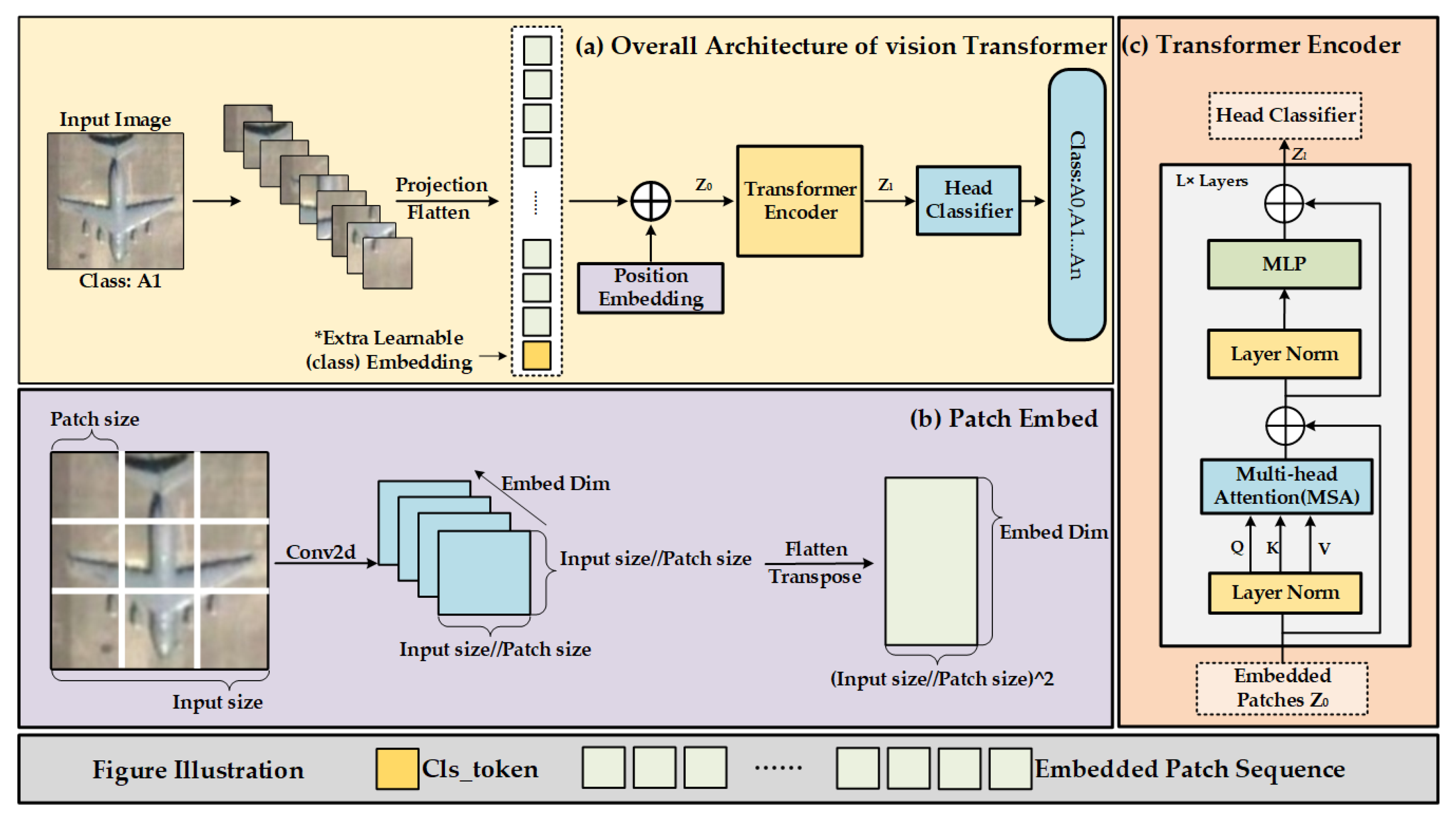
3.2. Review of Vision Transformer

ViT is a vanilla Transformer-based architecture [67], which has attracted much interest in recent years by showing SOTA performance in computer vision. Initially, the Transformer is used to solve natural language processing (NLP) problems using an encoder-decoder architecture with the ability to process sequential data in parallel, without relying on any recursive network. The core of the Transformer model is the self-attention mechanism, which is used to obtain the relationship between sequence elements. In recent years, Transformer has been found to be equally suitable for dealing with computer vision problems. The ViT is proposed to extend traditional Transformers to image classification. Specifically, ViT uses Transformer’s encoder module to classify images by mapping them to semantic labels after being partitioned into a sequence of image patches. Unlike the traditional CNN architecture, ViT focuses on different regions of the image through the attention mechanism and integrates the description of global features. As shown in Figure 4, the ViT architecture consists of a patch embedding module, an encoder, and a head classifier.
First, as shown in Figure 4b, the input image with a size of c × h × w, where c refers to the input channels, h refers to the height of the image, and w refers to the width, will be partitioned into a sequence of 2D patches. Each patch has a dimension of c × p × p, and the length of the sequence is n, where n = h × w/ p 2 and p refers to the size of each image patch, typically set as 16 or 32. Then, each patch is flattened by a linear projection and mapped to dimension D ( X p n E). The author then prepends a learnable class embedding (cls_token) to the flattened patches ( Z 0 0 = X c l a s s ). As shown in Figure 4a, the cls_token is the 0 t h token prepended to the embedded patch sequence. The cls_token is completely randomly initialized and independent of the image information, so the learning tendency for a particular token in the sequence can be avoided. Then, as the image changes from a two-dimensional to a one-dimensional patch sequence, the spatial position information is lost. In addition, the internal operations in Transformer are positional independent. To retain positional information, standard learnable 1D position embeddings ( E p o s ) are added to the patch embedding. Finally, the embedded feature Z 0 (Equation (2)) is then fed into the Transformer encoder, as shown in Figure 4c. In Equation (2), z 0 refers to the concatenated tokens. C is the number of channels, P is the patch size, and D is the output dimensions of the trainable linear projection.
Z 0 = [ X c l a s s ; X p 1 E ; X p 2 E ; ; X p N E ] + E p o s , E R ( P 2 · C ) × D , E p o s R ( N + 1 ) × D
As shown in Figure 4c, each Transformer encoder consists of a multi-head self-attention (MSA) [20] and a multi-layer perception (MLP) (Equations (3) and (4)). LN represents the layernorm operation which is applied before every block; the stream output z l in the transformer encoder can be described as the following formulas, where L is the number of encoders in the sequence:
Z l = M S A ( L N ( z l 1 ) ) + z l 1 , l = 1 . . . L
Z l = M L P ( L N ( z l ) ) + z l , l = 1 . . . L

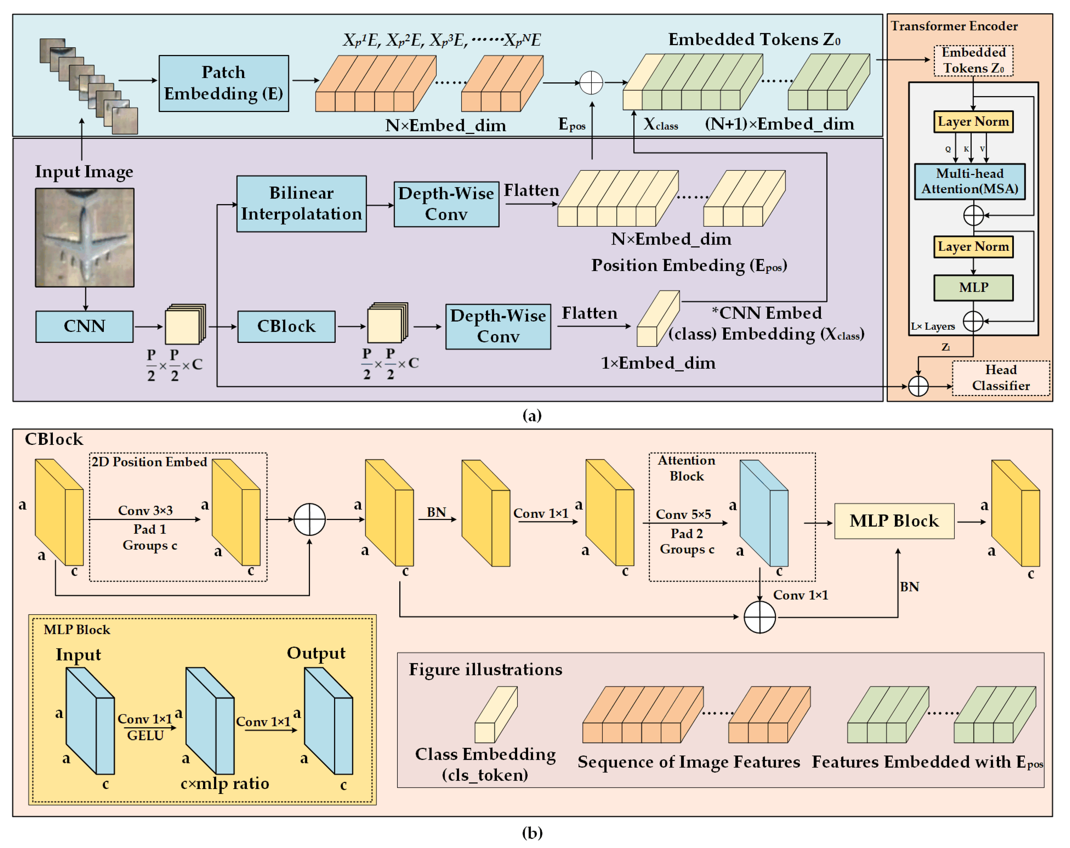
3.3. Plug-and-Play CNN Feature Embedded Hybrid Vision Transformer

As analyzed above, both CNN and ViT have certain shortcomings in feature representation. Generally, CNNs have poor capabilities to extract global context information due to the limited ERF, while ViT focuses on modeling the relationship between image patches and ignores the information within the patches. The self-attention mechanism makes ViT specialize in obtaining better global feature descriptions but is inferior to CNN for local feature representation. In addition, although the ViT structure can set up the global context information remarkably well, ViT models usually require extra data for pre-training to achieve fast convergence and obtain better performance. This is partly due to the structure of the Transformer itself, which lacks the inductive biases in CNNs, and partly due to the use of completely random initialization of the cls_token that is independent of the image information. The authors intended to address the Transformer’s tendency to learn for a particular image patch by a completely random initialization of cls_token, but it would cause the ViT to rely on a large amount of extra data pre-training before it could converge. This causes the training overhead of ViTs to be much higher than CNNs in practical applications. To solve the above problems, a plug-and-play CNN feature embedded hybrid vision transformer ( P 2 FEViT) is proposed in this paper, as shown in Figure 5.
The overall structure of P 2 FEViT is shown in Figure 5a. The input images are first fed in parallel to the patch embedding module and a CNN network. Unlike ViT, CNN gradually expands the receptive field by stacking convolution and pooling, and local features are described more richly. Consequently, we design a plug-and-play embedding module to introduce CNN features into the ViT structure to enhance the local feature representation. Notably, CNN features as a plug-and-play module can be obtained from any CNN structure, adding flexibility to our proposed network structure. The CNN-extracted features are fed into two parallel branches. In the first branch, the CNN-extracted features are fed into the CBlock, as shown in Figure 5b. It is designed to add 2D-attention information through depth-wise convolution and smoothly blend CNN features with ViT. The output feature of CBlock is mapped to the same dimension as the ViT embedded dimension through depth-wise convolution and then flattened. The flattened features are used as the extra learnable embedding ( X c l a s s ) and prepended to the embedded patches in ViT, as shown in Equation (5). In Equation (5), Ker refers to the 2-d depth-wise convolution, and i refers to the CNN-extracted features.
X c l a s s = K e r 7 × 7 ( C B l o c k ( i ) ) , X c l a s s R 1 × D
In the other branch, the CNN-extracted feature is first up-sampled to the same size as the image patches in ViT. Then, the depth-wise convolution is used to adjust the output dimension. The output feature is applied as the position embedding ( E p o s , Equation (6)) and added to the patch embeddings in ViT (Equation (7)). Finally, the embedded feature sequence Z 0 can be obtained according to Equation (7).
E p o s = K e r 3 × 3 ( U p s a m p l e ( i ) ) , E p o s R N × D
Z 0 = { X c l a s s ; [ ( X p 1 E ; X p 2 E ; ; X p N E ) + E p o s ] } , E R ( P 2 · C ) × D
Since CNN focuses more on the description of local information and ViT focuses more on the integration of global features, the features can be complementary by combining two different feature descriptions of CNN and ViT. In addition, the authors of ViT proposed that the purpose of initializing the cls_token completely randomly is to enable each token to obtain the same learning tendency and, therefore, set the cls_token to be independent of image features. However, in our approach, embedding tokens based on the CNN extracted features are added to the ViT structure as the cls_token and position embedding. The design objectives are as follows: First, the cls_token is derived from CNN-extracted features, which describes the overall features of the input image rather than the features corresponding to a certain patch and, thus, does not cause excessive learning propensity for a specific token. Second, the cls_token is based on a CNN description of the image features rather than a completely random initialization, so that inductive biases can be introduced and the Transformer encoder can converge faster as well as reduce training costs. In addition, the position embedding is based on the CNN-extracted features instead of a randomly initialized vector, which is more conducive to rapid convergence. The hybrid embedded feature is then fed into the Transformer encoder to model the global context information. Third, the feature-embedded ViT can be constructed by any two existing CNN and ViT models. The newly constructed model does not need to be pre-trained on a very large image classification dataset, such as JFT-300M [65]. Fast convergence can be achieved by directly using the pre-trained models of the sub-networks. Our plug-and-play network construction approach can save a lot of training costs in practical applications.

3.4. Head Classifier

To obtain the final RSIC results, we cascade a head classifier with the Transformer encoder. As shown in Figure 5a, the hybrid feature of the Transformer encoder’s output and CNN-extracted feature ( Z C N N ) is fed into the fully connected (FC) layer and softmax layer in the head classifier after layer normalization to obtain the final classification confidence p (Equations (8) and (9)). Z l 0 is the output state of cls_token at the L t h encoder.
y = L N ( z l 0 + Z C N N )
p = s o f t m a x ( F C ( y ) )
In addition, we use the cross-entropy function as the training loss function of our network, as shown in Equation (10), where c i is the i t h element of ground-truth for category c. p i is the predicted classification confidence, and N is the total number of categories.
L C E = i = 1 N c i l o g ( p i )

4. Experiments and Analysis

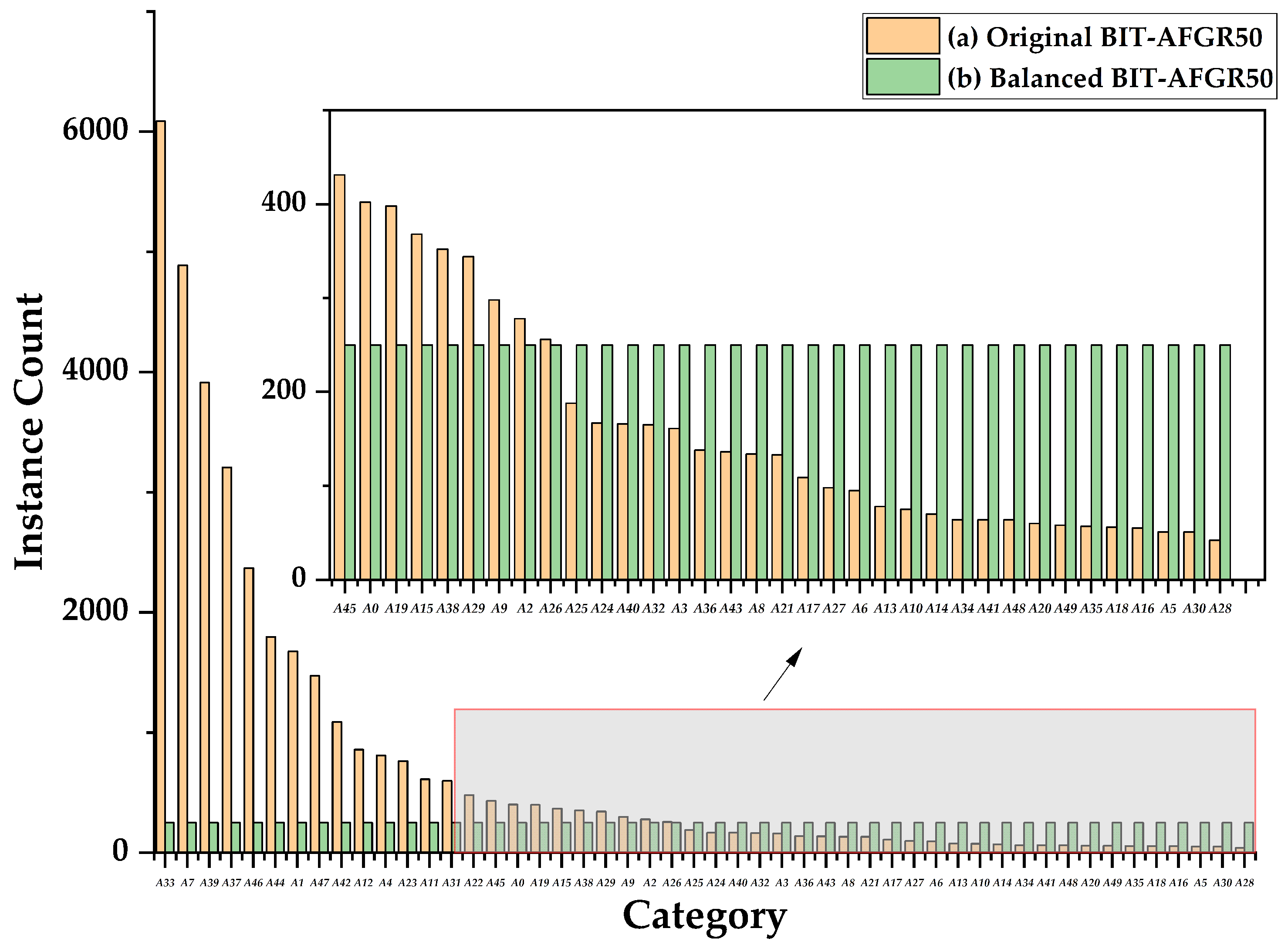
4.1. Establishment of BIT-AFGR50
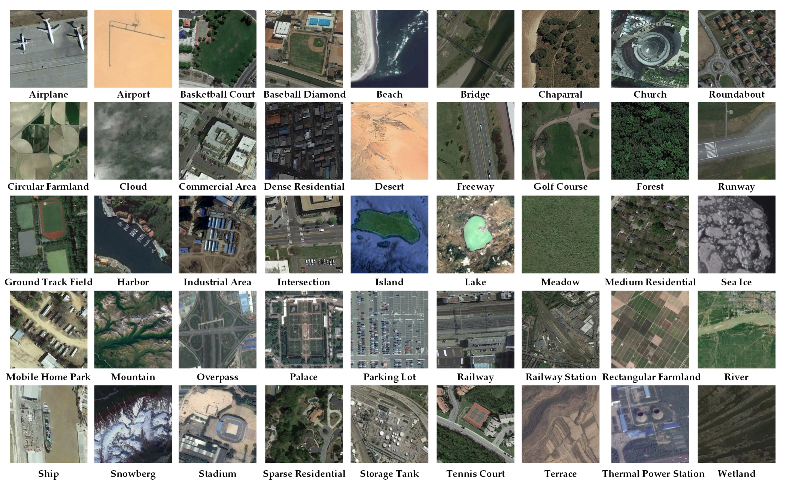
To construct a challenging aircraft fine-grained recognition dataset, we collected a large amount of optical remote sensing data from Google Earth. The collected images contain 50 categories of aircraft targets with various resolutions. At the same time, a large amount of historical image data from airports was collected to enrich the aircraft category diversity. In addition, the fine-grained aircraft category was annotated by professionals to ensure annotation accuracy. The original BIT-AFGR50 contains 36,278 image instances with 50 categories, and the original resolution were maintained for each category of aircraft instance.
Considering the realistic existence of each category of aircraft targets, the number of each category in the originally constructed dataset was unbalanced where a long-tail distribution exists. The instance number distribution of each category is shown in Figure 6. To more intuitively verify the effectiveness of the proposed hybrid network in terms of feature representation, we balanced the dataset to remove the effect of long-tail distribution on classifier training. We constructed the balanced classification dataset by means of data augmentation methods, such as random flipping, rotation, brightness adjustment, random sampling, etc. In the balanced BIT-AFGR50, the number of aircraft categories remained at 50, and the total sample instances were 12,500, of which each category had a sample of 250 aircraft instances. The balanced dataset is more suitable for academic research on deep learning-based methods, as it contains enough images with balanced and sufficient sample instances of each category. The variation in image instances between the original and balanced BIT-AFGR dataset is shown in Figure 6. The proposed BIT-AFGR50 can compensate for the current lack of datasets in fine-grained aircraft recognition. A comparison of our proposed BIT-AFGR50 with other publicly available optical remote sensing classification datasets is shown in the following table. Both the original and the balanced dataset will be available at https://github.com/wgqqgw/BIT-KTYG-AFGR ( accessed on 25 March 2023). The relationship between the realistic category name (e.g., F/A-18) and its annotation (A33) in the dataset will be published on our website as well. Figure 7 shows examples of aircraft targets in BIT-AFGR50. In addition, we provide several official train-test data partition schemes, such as train:test = 1:9, train:test = 2:8, etc. Both specific dataset partition schemes are available on our website for researchers to use in different tasks. Comparisons among publicly available optical RSIC datasets are shown in Table 1.

4.2. Datasets

To validate the effectiveness of our proposed P 2 FEViT, we conducted a series of experiments on several remote sensing classification datasets. The details of the datasets used are as follows:
NWPU-RESISC45 (NWPU-R45) [24]: The NWPU-R45 dataset contains 31,500 images with 45 classes of remote sensing scene targets, each containing 700 samples. The size of each image instance is fixed at 256 × 256, and the spatial resolution ranges from 0.2 to 30 m. We adopt 10% and 20% training ratios in our experiments based on the common practice in the remote sensing image classification literature [25,34,56,68,69,70,71,72]. Since using a smaller training set is a challenging scenario, it allows us to test the robustness and generalization capabilities of our proposed method. Additionally, a limited training set is a realistic representation of the scarcity of labeled data often faced in real-world remote sensing applications. Consequently, we randomly selected 10% and 20% samples as the training data for experiments. Samples of NWPU-R45 are shown in Figure 8.
BIT-AFGR50: The BIT-AFGR50 dataset contains 12,500 images of 50 classes of aircraft targets, each containing 250 image instances. The size of each image instance is fixed at 128 × 128, and the spatial resolution ranges from 0.5 to 1 m. Three data partitioning schemes are adopted to further explore the generalization capability and robustness of our method. We randomly selected 10%, 20%, and 30% of the images as training data to conduct experiments, respectively. The rest 90%, 80%, and 70% were used as test data to evaluate the RSIC performance.

4.3. Experiment Setup

In our experiments, we selected two typical CNN structures, the classical ResNet50 and EfficientNet, to obtain the embedded features. The embedded CNN feature was fused with typical ViT structures to construct our plug-and-play P 2 FEViT. In the training phase, all training samples were normalized to 224 × 224 RGB images. AdamW was adopted as the network update optimizer in 400 epochs. The batch size, weight decay, and decay epoch were set to 160, 0.05, and 30, respectively. The initial learning rate was set to 0.0005, and a cosine policy approach was used for a 5-epoch warm-up. The GPU resources used were two blocks of TITAN RTX.

4.4. Evaluation Metrics

In the experiments, the overall accuracy (OA) and confusion matrix (CM) were applied to evaluate the classification performance. The details are as follows:
(1)
OA: overall accuracy (OA) is defined as the ratio of correctly classified and total samples. It can be calculated as follows:
O A = 1 N i N f ( i )
where N represents the total number of image samples in the dataset. f(i) refers to the classification accuracy of the ith sample. If correctly classified, then f(i) equals 1 and vice versa 0. In addition, the OA on each remote sensing classification dataset is the average of five repeated runs.
(2)
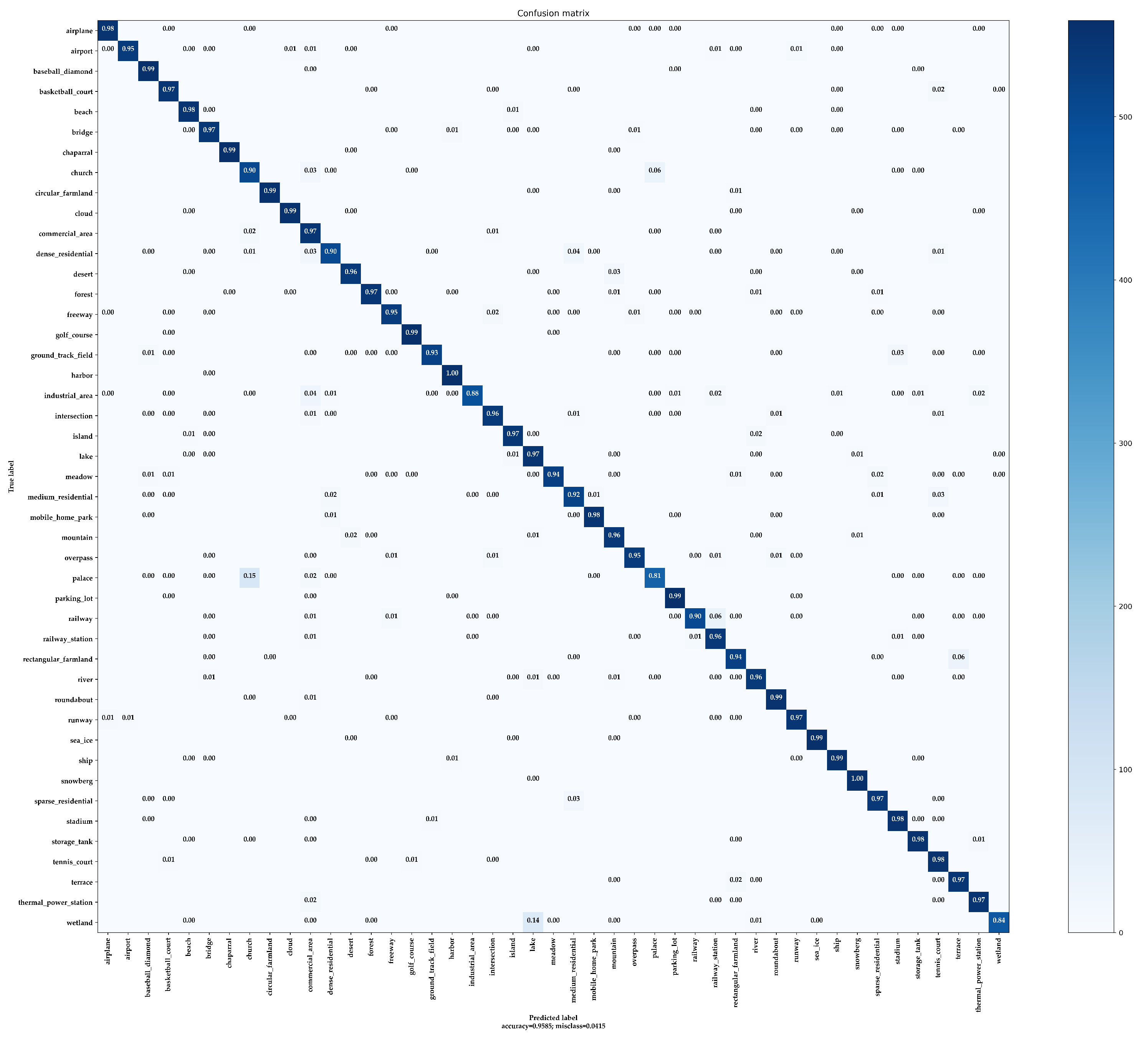
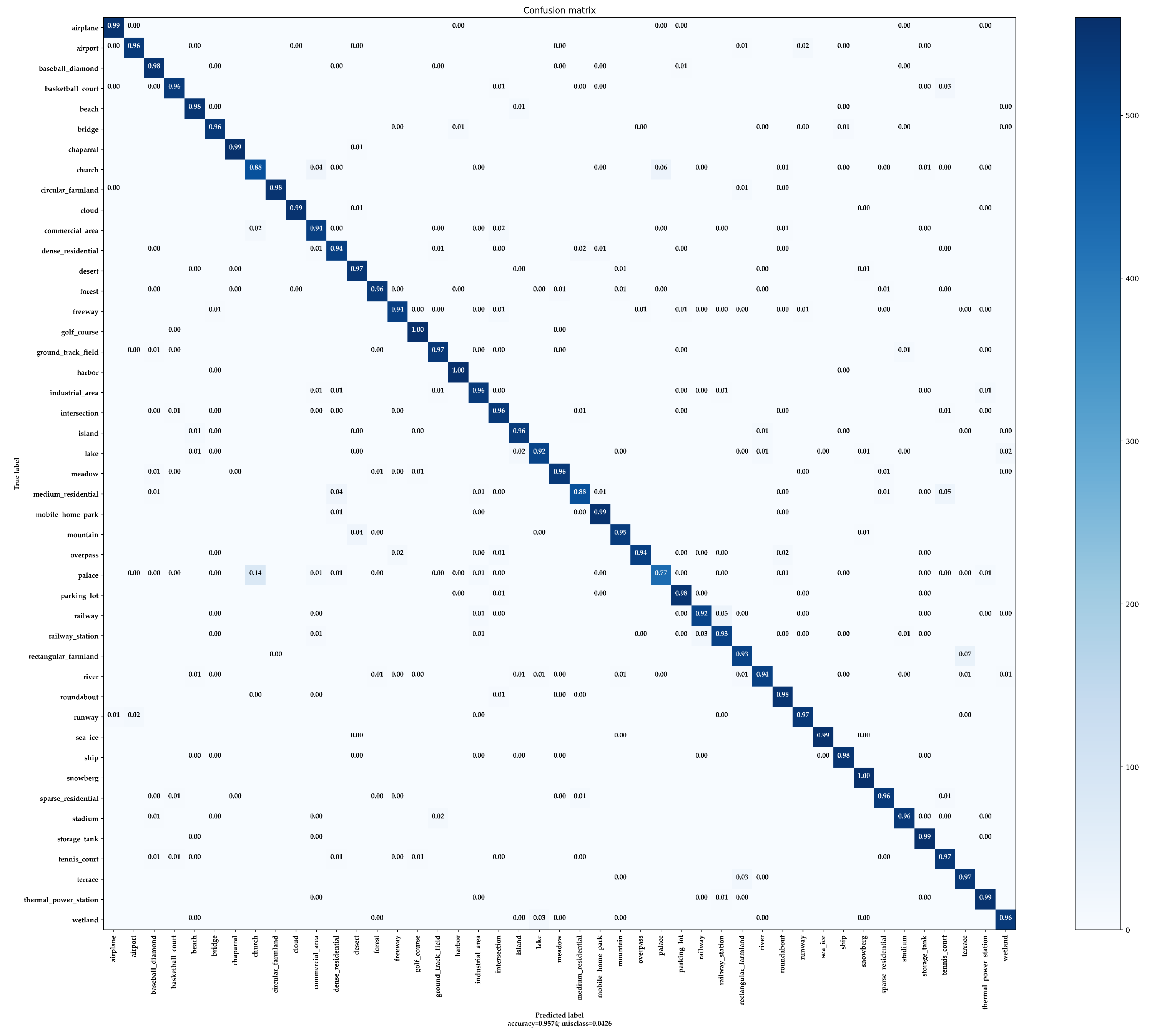
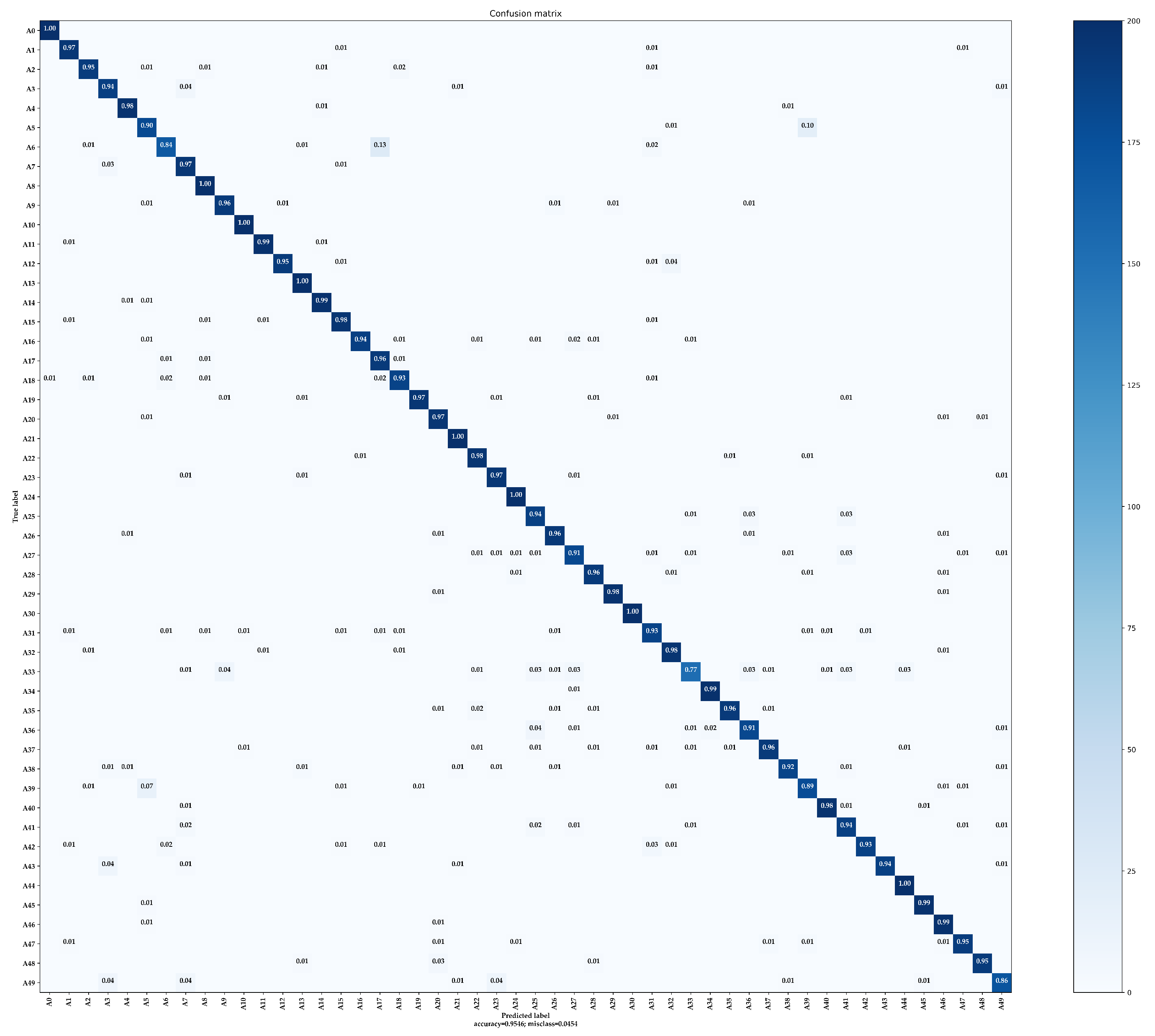
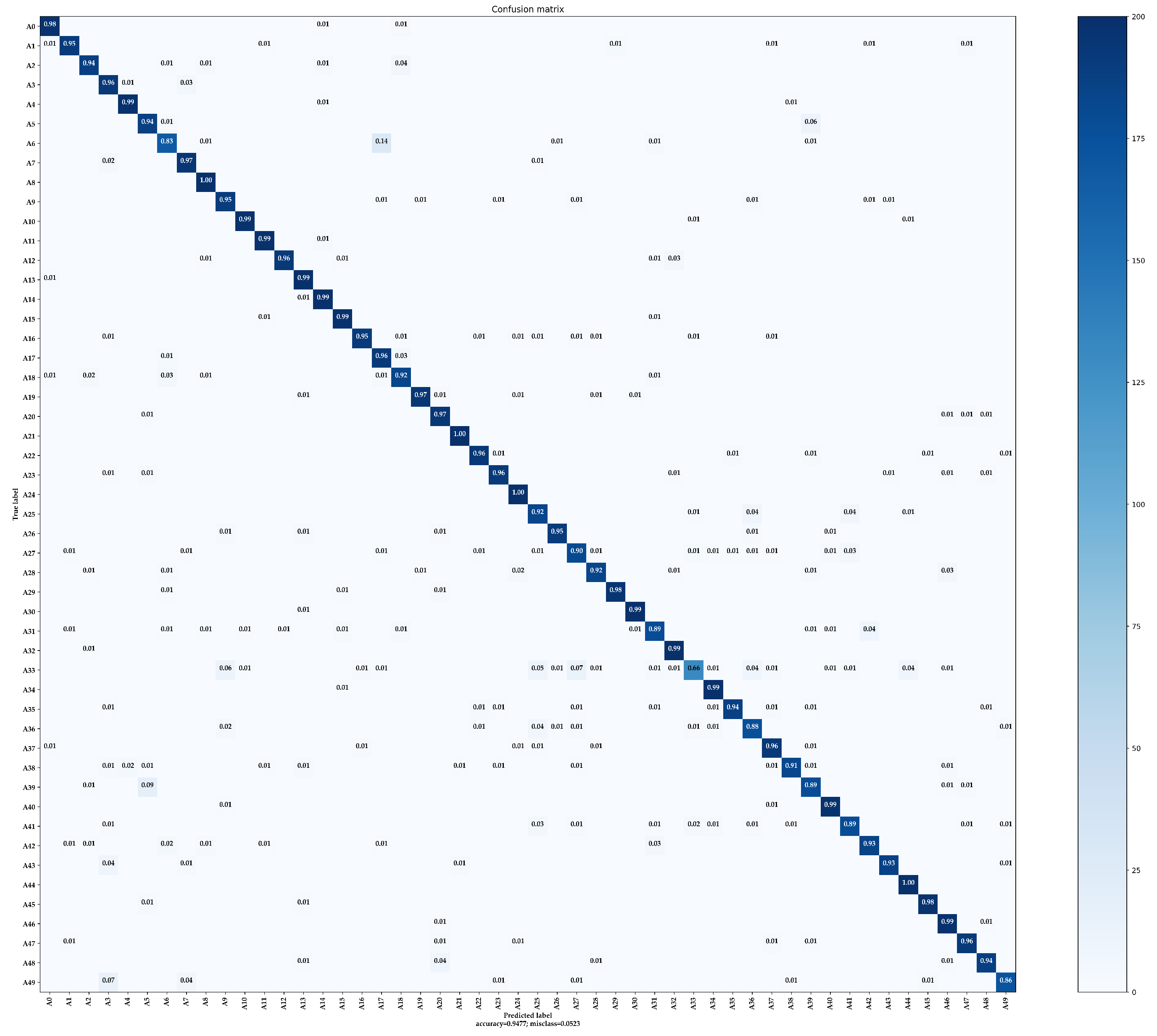
CM: The confusion matrix is a standard format for image classification accuracy evaluation and consists of a matrix with N rows and N columns, where N denotes the total number of categories. The columns in the confusion matrix represent the predicted categories, and the total number of each column represents the total number of images predicted for that category. The rows indicate the ground truth attribution category, and the total number of each row indicates the total number of images belonging to that category in the test set. The confusion matrix is mainly used to visually compare the classification prediction results with the ground truth values.

4.5. Performance Evaluation and Ablation Studies

To evaluate the classification performance of the proposed P 2 FEViT, comparison experiments against several SOTA classification methods were conducted on NWPU-R45 [24]. As shown in Table 2, the proposed P 2 FEViT achieved the highest OA of 94.97% and 95.85%, with 10% and 20% training ratios, respectively. As shown in Table 2, our P 2 FEViT achieved the optimal classification overall accuracy (OA) on the NWPU-R45 dataset [24]. When dealing with the NWPU-R45 remote sensing scene classification dataset, we need to obtain both global contextual information to describe larger scene targets, and also to consider local features to cope with the potent inter-class similarity and intra-class variability. SDAResNet [68] proposed a dual saliency attention residual network to set up both channel and spatial information for RSIC. SCCov [69] applied the skip-connections to integrate multi-scale features, which is beneficial to address the large-scale variance in RSIC. ACNet [71] designed a CNN-based attention-consistent network to explore the global features from remote-sensing images. Constrained by CNN’s limited receptive field, they are still not able to obtain extensive enough global information. A self-attention mechanism is used in [25,34,56,68] to capture the global context information. The GLANet [68] applied the attention mechanism to obtain global information using a squeeze-excitation module. Lv et al. [34] integrate a channel attention module with the MSA to model global information as well as considering the channel attention in the cls_token. Cheng et al. [25] obtain global context information through a series of hidden Markov models. However, the methods focus more on the relationship between sequenced patches and ignore the local information inside them.
Compared with the recent SOTA RSIC methods, the overall accuracy of our method P 2 FEViT(ViT-B/EfficientB0) is 1.29%, 0.34% higher than study [25] under the condition of 10% and 20% training ratios, respectively. In addition, the classification performance of our proposed P 2 FEViT is improved compared with that of its sub-network plug-ins. For example, the overall accuracy of P 2 FEViT(ViT-B/ResNet50) is 0.79% and 1.52% higher than its sub-network ViT-B/16 and ResNet50, respectively.
The confusion matrixes (CM) of our proposed P 2 FEViT ( P 2 FEViT (ViT-B/EffcientB0) and P 2 FEViT (VT-B/ResNet50)) on the NWPU-R45 [24] at 20% training ratio are shown in Figure 9 and Figure 10. It can intuitively show the classification performance of our mehtod. The diagonal line indicates the percentage correctly classified.
For the 45 classes in the NWPU-R45 [24], most of them obtained classification accuracy above 90%. For P 2 FEViT (ViT-B/EffcientB0), the accuracy of 36 categories was more than 95%, while only “palace” and “wetland” were less accurate. The accuracy rates for these two pair of categories were as low as 81% and 84%, respectively. Because of the potent intra-class variation and little inter-class difference, as shown in Figure 11, the targets in category “palace” and “wetland” were easily classified into “church” and “lake”. For P 2 FEViT (ViT-B/ResNet50), the accuracy of 33 categories was more than 95%. The classification results show that different structures of CNNs focus differently on feature description. For example, the accuracy of “wetland” in P 2 FEViT (ViT-B/ResNet50) is much higher than that in P 2 FEViT (ViT-B/EffcientB0), but the “medium_residential” is more confused. Consequently, our plug-and-play architecture can be constructed with the practical application’s requirements to create an optimal structure for that task.
As analyzed in this paper, the proposed P 2 FEViT makes full use of the complementary feature descriptions of CNN and ViT by embedding the CNN-extracted features into the ViT model. The CNN-extracted features can lead to fast convergence of ViT through introducing the inductive biases, as well as enhancing the local feature description, thus improving the classification performance. To demonstrate the outstanding feature representation capability in our proposed method, a series of ablation studies were carried out on the remote sensing fine-grained dataset, BIT-AFGR50. As shown in Table 3, we conducted experiments on the classical CNN classification network and ViT model on BIT-AFGR50 with a 20% training ratio first. When processing the BIT-AFGR50 dataset, the stronger inter-class similarity of the targets in the fine-grained recognition task requires the network to have more powerful feature representation capabilities. For the hybrid P 2 FEViT, the fine-grained recognition task focuses more on better integrating the CNN description of local features into the ViT model to obtain the optimal feature representation capability.
As a result, the hybrid P 2 FEViT (ViT-S/EfficientB3) obtains an optimal classification result of 95.46%. Compared with its CNN/ViT sub-networks, the classification performance is improved by 1.45% and 2.64%, respectively. In addition, we further explore the effect of the proposed hybrid model on the convergence of ViT. As shown in Figure 12 and Table 3, the hybrid P 2 FEViT can obtain the same classification performance as the original ViT model in much fewer iteration epochs. For example, as shown in Table 3, the proposed hybrid ViT model constructed by fusing two plug-and-play CNN features with ViT-S/16 trained 150 and 90 epochs, respectively, can obtain the same verification accuracy as the original ViT-S/16 trained 400 epochs. In addition, the overall accuracy of P 2 FEViT (ViT-B/EfficientB3) with 200 training epochs is comparable to that of ViT-B/16 with 400 training epochs. Figure 12a shows the overall accuracy of classical CNN/ViT and our proposed P 2 FEViT fine-tuned with the ImageNet [6] pre-trained weights. Figure 12b shows the overall accuracy of the above methods trained from scratch. It can be intuitively seen that, due to the complementary global-local feature representation in the proposed model, the classification performance can be significantly improved at the same iteration epoch. Furthermore, the proposed P 2 FEViT is able to converge faster than the original ViT model and obtain better performance when we do not have the conditions to pre-train on a large amount of additional data.
To further explore the feature generalization capability and robustness of the proposed method, we also conducted experiments with 10% and 30% training ratios on BIT-AFGR50. As shown in Table 4, compared with other CNN and ViT models, our proposed P 2 FEViT hybrid model, constructed by the above CNN and ViT models, can improve the overall accuracy by at least 0.75%, 0.55%, and 0.52% at 10%, 20%, and 30% training ratios, respectively. The overall accuracy growth decreased as the training sample ratio increased from 10% to 30%. This observation could be attributed to the fact that, with larger training sets, the models become better at capturing the underlying data distribution, and the additional benefits provided by our method may become less pronounced. This phenomenon is not necessarily an anomaly, but more likely reflects a general trend in real-world application scenarios. The performance of various methods tends to improve as the number of training samples increases, leading to a decrease in relative performance improvement. For methods that improve classification accuracy by enhancing the network’s feature description capability, the performance improvement may be more pronounced when there is less training data. When there is less training data, it may be difficult for the model to capture the underlying distribution of the data, so the performance improvement achieved by enhancing the feature description capability of the network can be significant. In addition, our method still demonstrates a performance improvement with a 30% training ratio, although the improvement is smaller than that observed at a 10% training ratio.
Figure 13 and Figure 14 illustrate our method’s confusion matrixes (CM) on the BIT-AFGR50 dataset with a 20% training ratio. Figure 13 illustrates the CM of our P 2 FEViT (ViT-S/EfficientB3) on BIT-AFGR50. A total of 47 aircraft categories out of the total 50 categories in the BIT-AFGR50 dataset achieved an accuracy higher than 90%, and 34 categories obtained the classification top-1 accuracy higher than 95%. Some categories, such as “A10”, “A24”, “A30” and “A34”, achieved outstanding classification performance higher than 98%.
Figure 14 illustrates the CM of our P 2 FEViT (ViT-S/ResNet50). A total of 43 out of the total 50 categories in the BIT-AFGR50 dataset achieved an accuracy higher than 90% and 32 of them obtained the top-1 accuracy higher than 95%. The most confusing category of our method in BIT-AFGR50 is “A33”. As shown in Figure 7, the “A33” aircraft targets refer to the “F/A-18” category with relatively low spatial resolution. In addition, the “A33” targets have high inter-class similarity to other fighter aircraft categories, which is difficult to distinguish correctly either by manual classification or deep learning. To verify the improvement in representation capability in our method, we also statistically analysed the top-1 accuracy of the most confused categories in the CNN/ViT sub-networks. Compared with our P 2 FEViT (ViT-S/EfficientB3), the accuracy of “A33” in ViT-S/16 was 68% and only 20 out of 50 total categories achieved accuracy higher than 95%, which is far inferior to our method. For the other sub-network EfficientNet-B3, the most confused category “A33” obtained the same top-1 accuracy with our method, but only 30 categories out of the total 50 categories obtained accuracy higher than 95%, which is not as good as our P 2 FEViT (ViT-S/EfficientB3).

5. Discussion

To demonstrate the effectiveness of P 2 FEViT, we compared the classification performance of ViT-S/16 with our method on the NWPU-R45 [24] and BIT-AFGR50 datasets, respectively. The experimental results are shown in Table 2 and Table 3. Compared with the ViT model, our proposed method showed significant improvement in both classification performance and convergence speed. Specifically, compared with the SOTA methods study [25,56] in RSIC, the accuracy was improved by 1.07% and 0.34% in the NWPU-R45 [24], with a training ratio of 10% and 20%, respectively. In the BIT-AFGR50 dataset, the training ratio was 20% and the plug-and-play hybrid ViT model’s accuracy was improved by 2.64% and 1.45% compared with the original ViT and CNN models.
At the same time, the training convergence speed was improved by 2∼3 times. To further explore the feature representation capability and robustness of our method, we also conducted experiments under different training ratios on the BIT-AFGR50 dataset. Although the overall accuracy growth decreased with increase in training data, our method still demonstrated performance improvements with all the training ratios.
In summary, the proposed P 2 FEViT with CNN-ViT feature fusion can achieve complementary features extracted by CNN and ViT, while avoiding the heavy dependence on a large amount of extra data for ViT-based model pre-training. The global-local features extracted by P 2 FEViT make the overall feature description more comprehensive so that the classification accuracy can be improved. To clearly compare the original ViT and the proposed method, we used feature maps of different methods for visualization through Grad-CAM [66]. The feature maps were obtained to display the regions with attention in the image.
The original image, attention maps of CNN, ViT and our P 2 FEViT(ViT-S/ResNet50) are shown in Figure 15, respectively. The original images are from the NWPU-R45 dataset for airplane, bridge, roundabout, tennis-court and runway. It can be intuitively seen from the figures that the attention of ViT can cover more global context information, whereas the attention on the local continuous regions is weak. The CNN model focuses more on the local feature description, but there is a lack of global context information. The proposed method can take into account both global and local features and construct a local-global complementary feature map.
Furthermore, we separately visualized the features of proposed P 2 FEViT(ViT-S/EfficientB3) and its sub-network ViT-S/16 and EfficientNet-B3 by t-SNE [74], which can map the distances of features in different categories into a 2-D space. The test images were from the fine-grained target recognition dataset, BIT-AFGR50. In Figure 16, we can clearly see that the proposed P 2 FEViT can reduce intra-class diversity as well as inter-class similarity. In the feature space, the proposed hybrid structure can obtain more distinguished features in different categories. Consequently, the proposed P 2 FEViT can significantly improve the classification performance of ViT on remote sensing images.

6. Conclusions

In this paper, we have proposed a plug-and-play CNN-feature embedded hybrid Vision Transformer ( P 2 FEViT). Unlike the original ViT model, the proposed P 2 FEViT embeds the CNN extracted features as embedded tokens into the ViT structure. The ViT model with strong global feature description capability is combined with the CNN model, which can be more adept at extracting local features. The local-global fusion strategy can help the hybrid network to learn features from different perspectives and achieve complementarity. In addition, we have established a remote sensing aircraft fine-grained recognition dataset, BIT-AFGR50, which is a comprehensive multi-class publicly available aircraft target fine-grained recognition dataset. The proposed method has been evaluated on two public remote-sensing image classification datasets, NWPU-R45, and BIT AFGR-50. The experimental results showed that our proposed method can build feature-embedded hybrid ViT structures from arbitrary ViT and CNN models by the method in this paper, which can effectively improve the convergence speed and classification performance. Our future work will further explore the approach to improve the performance of the ViT model and achieve lightweight computation.

Author Contributions

Conceptualization, G.W. and Y.Z.; data curation, G.W., T.Z. and Y.Z.; software, G.W.; validation G.W.; formal analysis, G.W. and Y.Z.; writing, G.W. and Y.Z.; writing-review and editing, G.W., Y.Z., H.C., L.C., S.Z., T.Z., H.D. and P.G. All authors have read and agreed to published version of the manuscript.

Funding

This work was supported by the National Science Foundation for Young Scientists of China under Grant 62101046, in part by the Space based on orbit real-time processing technology under grant 2018-JCJQ-ZQ-046, in part by the National Natural Science Foundation of China under Grant 62136001, and in part by the multi-source satellite data hardware acceleration computing method with low energy consumption under grant 2021YFA0715204.

Data Availability Statement

The NWPU-RESISC45 dataset in this study is openly and freely available at http://www.escience.cn/people/JunweiHan/NWPU-RESISC45.html (accessed on 1 November 2022). The BIT-AFGR50 dataset in this study will be openly and freely available at https://github.com/wgqqgw/BIT-KTYG-AFGR (accessed on 25 March 2023).

Conflicts of Interest

The authors declare no conflict of interest.

References

  1. Zhang, J.; Chen, L.; Wang, C.; Zhuo, L.; Tian, Q.; Liang, X. Road recognition from remote sensing imagery using incremental learning. IEEE Trans. Intell. Transp. Syst. 2017, 18, 2993–3005. [Google Scholar] [CrossRef]
  2. Abdullahi, H.S.; Sheriff, R.; Mahieddine, F. Convolution neural network in precision agriculture for plant image recognition and classification. In Proceedings of the 2017 Seventh International Conference on Innovative Computing Technology (INTECH), Luton, UK, 16–18 August 2017; IEEE: Piscataway, NJ, USA, 2017; Volume 10, pp. 256–272. [Google Scholar]
  3. Nielsen, M.M. Remote sensing for urban planning and management: The use of window-independent context segmentation to extract urban features in Stockholm. Comput. Environ. Urban Syst. 2015, 52, 1–9. [Google Scholar] [CrossRef]
  4. Qin, P.; Cai, Y.; Liu, J.; Fan, P.; Sun, M. Multilayer feature extraction network for military ship detection from high-resolution optical remote sensing images. IEEE J. Sel. Top. Appl. Earth Obs. Remote Sens. 2021, 14, 11058–11069. [Google Scholar] [CrossRef]
  5. Mirik, M.; Ansley, R.J. Utility of Satellite and Aerial Images for Quantification of Canopy Cover and Infilling Rates of the Invasive Woody Species Honey Mesquite (Prosopis Glandulosa) on Rangeland. Remote. Sens. 2012, 4, 1947–1962. [Google Scholar] [CrossRef] [Green Version]
  6. Deng, J.; Dong, W.; Socher, R.; Li, L.J.; Li, K.; Fei-Fei, L. Imagenet: A large-scale hierarchical image database. In Proceedings of the 2009 IEEE Conference on Computer Vision and Pattern Recognition, Miami, FL, USA, 20–25 June 2009; IEEE: Piscataway, NJ, USA, 2009; pp. 248–255. [Google Scholar]
  7. Krizhevsky, A.; Hinton, G. Learning Multiple Layers of Features from Tiny Images; University of Toronto: Toronto, ON, Canada, 2009. [Google Scholar]
  8. Xiao, H.; Rasul, K.; Vollgraf, R. Fashion-mnist: A novel image dataset for benchmarking machine learning algorithms. arXiv 2017, arXiv:1708.07747. [Google Scholar]
  9. LeCun, Y.; Bottou, L.; Bengio, Y.; Haffner, P. Gradient-based learning applied to document recognition. Proc. IEEE 1998, 86, 2278–2324. [Google Scholar] [CrossRef] [Green Version]
  10. Krizhevsky, A.; Sutskever, I.; Hinton, G.E. Imagenet classification with deep convolutional neural networks. Commun. ACM 2017, 60, 84–90. [Google Scholar] [CrossRef] [Green Version]
  11. Simonyan, K.; Zisserman, A. Very deep convolutional networks for large-scale image recognition. arXiv 2014, arXiv:1409.1556. [Google Scholar]
  12. Szegedy, C.; Liu, W.; Jia, Y.; Sermanet, P.; Reed, S.; Anguelov, D.; Erhan, D.; Vanhoucke, V.; Rabinovich, A. Going deeper with convolutions. In Proceedings of the IEEE Conference on Computer Vision and Pattern Recognition, Boston, MA, USA, 7–12 June 2015; pp. 1–9. [Google Scholar]
  13. Lowe, D.G. Distinctive image features from scale-invariant keypoints. Int. J. Comput. Vis. 2004, 60, 91–110. [Google Scholar] [CrossRef]
  14. Bay, H.; Tuytelaars, T.; Van Gool, L. Surf: Speeded up robust features. Lect. Notes Comput. Sci. 2006, 3951, 404–417. [Google Scholar]
  15. DARAL, N. Histograms of oriented gradients for human detection. In Proceedings of the 2005 IEEE Computer Society Conference on Computer Vision and Pattern Recognition (CVPR’05), San Diego, CA, USA, 20–25 June 2005; pp. 886–893. [Google Scholar]
  16. He, K.; Zhang, X.; Ren, S.; Sun, J. Deep residual learning for image recognition. In Proceedings of the IEEE Conference on Computer Vision and Pattern Recognition, Las Vegas, NV, USA, 27–30 June 2016; pp. 770–778. [Google Scholar]
  17. Brock, A.; De, S.; Smith, S.L.; Simonyan, K. High-performance large-scale image recognition without normalization. In Proceedings of the International Conference on Machine Learning, Virtual, 18–24 July 2021; pp. 1059–1071. [Google Scholar]
  18. Liu, Z.; Mao, H.; Wu, C.Y.; Feichtenhofer, C.; Darrell, T.; Xie, S. A convnet for the 2020s. In Proceedings of the IEEE/CVF Conference on Computer Vision and Pattern Recognition, New Orleans, LA, USA, 18–24 June 2022; pp. 11976–11986. [Google Scholar]
  19. Zhang, H.; Wu, C.; Zhang, Z.; Zhu, Y.; Lin, H.; Zhang, Z.; Sun, Y.; He, T.; Mueller, J.; Manmatha, R.; et al. Resnest: Split-attention networks. In Proceedings of the IEEE/CVF Conference on Computer Vision and Pattern Recognition, New Orleans, LA, USA, 18–24 June 2022; pp. 2736–2746. [Google Scholar]
  20. Dosovitskiy, A.; Beyer, L.; Kolesnikov, A.; Weissenborn, D.; Zhai, X.; Unterthiner, T.; Dehghani, M.; Minderer, M.; Heigold, G.; Gelly, S.; et al. An image is worth 16x16 words: Transformers for image recognition at scale. arXiv 2020, arXiv:2010.11929. [Google Scholar]
  21. Liu, Z.; Lin, Y.; Cao, Y.; Hu, H.; Wei, Y.; Zhang, Z.; Lin, S.; Guo, B. Swin transformer: Hierarchical vision transformer using shifted windows. In Proceedings of the IEEE/CVF International Conference on Computer Vision, Montreal, BC, Canada, 11–17 October 2021; pp. 10012–10022. [Google Scholar]
  22. Zhou, D.; Kang, B.; Jin, X.; Yang, L.; Lian, X.; Jiang, Z.; Hou, Q.; Feng, J. Deepvit: Towards deeper vision transformer. arXiv 2021, arXiv:2103.11886. [Google Scholar]
  23. Chen, C.F.R.; Fan, Q.; Panda, R. Crossvit: Cross-attention multi-scale vision transformer for image classification. In Proceedings of the IEEE/CVF International Conference on Computer Vision, Montreal, BC, Canada, 11–17 October 2021; pp. 357–366. [Google Scholar]
  24. Cheng, G.; Han, J.; Lu, X. Remote sensing image scene classification: Benchmark and state of the art. Proc. IEEE 2017, 105, 1865–1883. [Google Scholar] [CrossRef] [Green Version]
  25. Cheng, X.; Lei, H. Remote sensing scene image classification based on mmsCNN–HMM with stacking ensemble model. Remote Sens. 2022, 14, 4423. [Google Scholar] [CrossRef]
  26. Wang, D.; Lan, J. A deformable convolutional neural network with spatial-channel attention for remote sensing scene classification. Remote Sens. 2021, 13, 5076. [Google Scholar] [CrossRef]
  27. Li, L.; Liang, P.; Ma, J.; Jiao, L.; Guo, X.; Liu, F.; Sun, C. A multiscale self-adaptive attention network for remote sensing scene classification. Remote Sens. 2020, 12, 2209. [Google Scholar] [CrossRef]
  28. Zhang, C.; Chen, Y.; Yang, X.; Gao, S.; Li, F.; Kong, A.; Zu, D.; Sun, L. Improved remote sensing image classification based on multi-scale feature fusion. Remote Sens. 2020, 12, 213. [Google Scholar] [CrossRef] [Green Version]
  29. Shen, J.; Yu, T.; Yang, H.; Wang, R.; Wang, Q. An Attention Cascade Global–Local Network for Remote Sensing Scene Classification. Remote Sens. 2022, 14, 2042. [Google Scholar] [CrossRef]
  30. Xu, K.; Huang, H.; Deng, P. Remote Sensing Image Scene Classification Based on Global–Local Dual-Branch Structure Model. IEEE Geosci. Remote Sens. Lett. 2022, 19, 1–5. [Google Scholar] [CrossRef]
  31. Luo, W.; Li, Y.; Urtasun, R.; Zemel, R. Understanding the effective receptive field in deep convolutional neural networks. Adv. Neural Inf. Process. Syst. 2016, 29. [Google Scholar]
  32. Ding, X.; Zhang, X.; Han, J.; Ding, G. Scaling up your kernels to 31x31: Revisiting large kernel design in cnns. In Proceedings of the IEEE/CVF Conference on Computer Vision and Pattern Recognition, 2022, New Orleans, LA, USA, 18–24 June 2022; pp. 11963–11975. [Google Scholar]
  33. Bazi, Y.; Bashmal, L.; Rahhal, M.M.A.; Dayil, R.A.; Ajlan, N.A. Vision transformers for remote sensing image classification. Remote Sens. 2021, 13, 516. [Google Scholar] [CrossRef]
  34. Lv, P.; Wu, W.; Zhong, Y.; Du, F.; Zhang, L. SCViT: A Spatial-Channel Feature Preserving Vision Transformer for Remote Sensing Image Scene Classification. IEEE Trans. Geosci. Remote Sens. 2022, 60, 1–12. [Google Scholar] [CrossRef]
  35. Penatti, O.A.; Nogueira, K.; Dos Santos, J.A. Do deep features generalize from everyday objects to remote sensing and aerial scenes domains? In Proceedings of the IEEE Conference on Computer Vision and Pattern Recognition Workshops, Boston, MA, USA, 7–12 June 2015; pp. 44–51. [Google Scholar]
  36. Yang, Y.; Newsam, S. Bag-of-visual-words and spatial extensions for land-use classification. In Proceedings of the 18th SIGSPATIAL International Conference on Advances in Geographic Information Systems, San Jose, CA, USA, 2–5 November 2010; pp. 270–279. [Google Scholar]
  37. Zhang, Y.; Wu, L.; Neggaz, N.; Wang, S.; Wei, G. Remote-Sensing Image Classification Based on an Improved Probabilistic Neural Network. Sensors 2009, 9, 7516–7539. [Google Scholar] [CrossRef] [PubMed] [Green Version]
  38. Han, M.; Liu, B. Ensemble of extreme learning machine for remote sensing image classification. Neurocomputing 2015, 149, 65–70. [Google Scholar] [CrossRef]
  39. Fauvel, M.; Tarabalka, Y.; Benediktsson, J.A.; Chanussot, J.; Tilton, J.C. Advances in Spectral-Spatial Classification of Hyperspectral Images. Proc. IEEE 2013, 101, 652–675. [Google Scholar] [CrossRef] [Green Version]
  40. Song, W.; Cong, Y.; Zhang, Y.; Zhang, S. Wavelet Attention ResNeXt Network for High-resolution Remote Sensing Scene Classification. In Proceedings of the 2022 17th International Conference on Control, Automation, Robotics and Vision (ICARCV), Singapore, 11–13 December 2022; IEEE: Piscataway, NJ, USA, 2022; pp. 330–333. [Google Scholar]
  41. Wang, H.; Gao, K.; Min, L.; Mao, Y.; Zhang, X.; Wang, J.; Hu, Z.; Liu, Y. Triplet-Metric-Guided Multi-Scale Attention for Remote Sensing Image Scene Classification with a Convolutional Neural Network. Remote Sens. 2022, 14, 2794. [Google Scholar] [CrossRef]
  42. Shi, C.; Zhao, X.; Wang, L. A multi-branch feature fusion strategy based on an attention mechanism for remote sensing image scene classification. Remote Sens. 2021, 13, 1950. [Google Scholar] [CrossRef]
  43. Miao, W.; Geng, J.; Jiang, W. Multi-Granularity Decoupling Network with Pseudo-Label Selection for Remote Sensing Image Scene Classification. IEEE Trans. Geosci. Remote. Sens. 2023, 61, 1. [Google Scholar] [CrossRef]
  44. Singh, A.; Bruzzone, L. Data Augmentation Through Spectrally Controlled Adversarial Networks for Classification of Multispectral Remote Sensing Images. In Proceedings of the IGARSS 2022-2022 IEEE International Geoscience and Remote Sensing Symposium, Kuala Lumpur, Malaysia, 17–22 July 2022; pp. 651–654. [Google Scholar] [CrossRef]
  45. Stivaktakis, R.; Tsagkatakis, G.; Tsakalides, P. Deep learning for multilabel land cover scene categorization using data augmentation. IEEE Geosci. Remote Sens. Lett. 2019, 16, 1031–1035. [Google Scholar] [CrossRef]
  46. Xiao, Q.; Liu, B.; Li, Z.; Ni, W.; Yang, Z.; Li, L. Progressive data augmentation method for remote sensing ship image classification based on imaging simulation system and neural style transfer. IEEE J. Sel. Top. Appl. Earth Obs. Remote Sens. 2021, 14, 9176–9186. [Google Scholar] [CrossRef]
  47. Yu, X.; Wu, X.; Luo, C.; Ren, P. Deep learning in remote sensing scene classification: A data augmentation enhanced convolutional neural network framework. GIScience Remote Sens. 2017, 54, 741–758. [Google Scholar] [CrossRef] [Green Version]
  48. Zhang, Y.; Liu, K.; Dong, Y.; Wu, K.; Hu, X. Semisupervised Classification Based on SLIC Segmentation for Hyperspectral Image. IEEE Geosci. Remote. Sens. Lett. 2020, 17, 1440–1444. [Google Scholar] [CrossRef]
  49. Yessou, H.; Sumbul, G.; Demir, B. A comparative study of deep learning loss functions for multi-label remote sensing image classification. In Proceedings of the IGARSS 2020-2020 IEEE International Geoscience and Remote Sensing Symposium, Waikoloa, HI, USA, 26 September–2 October 2020; IEEE: Piscataway, NJ, USA, 2020; pp. 1349–1352. [Google Scholar]
  50. Bazi, Y.; Al Rahhal, M.M.; Alhichri, H.; Alajlan, N. Simple yet effective fine-tuning of deep CNNs using an auxiliary classification loss for remote sensing scene classification. Remote Sens. 2019, 11, 2908. [Google Scholar] [CrossRef] [Green Version]
  51. Zhang, J.; Lu, C.; Wang, J.; Yue, X.G.; Lim, S.J.; Al-Makhadmeh, Z.; Tolba, A. Training convolutional neural networks with multi-size images and triplet loss for remote sensing scene classification. Sensors 2020, 20, 1188. [Google Scholar] [CrossRef] [Green Version]
  52. Zhang, J.; Zhang, M.; Pan, B.; Shi, Z. Semisupervised center loss for remote sensing image scene classification. IEEE J. Sel. Top. Appl. Earth Obs. Remote Sens. 2020, 13, 1362–1373. [Google Scholar] [CrossRef]
  53. Wei, T.; Wang, J.; Liu, W.; Chen, H.; Shi, H. Marginal center loss for deep remote sensing image scene classification. IEEE Geosci. Remote Sens. Lett. 2019, 17, 968–972. [Google Scholar] [CrossRef]
  54. Wang, D.; Zhang, Q.; Xu, Y.; Zhang, J.; Du, B.; Tao, D.; Zhang, L. Advancing plain vision transformer towards remote sensing foundation model. IEEE Trans. Geosci. Remote. Sens. 2022. [Google Scholar] [CrossRef]
  55. Sha, Z.; Li, J. MITformer: A Multiinstance Vision Transformer for Remote Sensing Scene Classification. IEEE Geosci. Remote Sens. Lett. 2022, 19, 1–5. [Google Scholar] [CrossRef]
  56. Deng, P.; Xu, K.; Huang, H. When CNNs Meet Vision Transformer: A Joint Framework for Remote Sensing Scene Classification. IEEE Geosci. Remote Sens. Lett. 2022, 19, 1–5. [Google Scholar] [CrossRef]
  57. Gao, P.; Lu, J.; Li, H.; Mottaghi, R.; Kembhavi, A. Container: Context aggregation network. arXiv 2021, arXiv:2106.01401. [Google Scholar]
  58. Dai, Z.; Liu, H.; Le, Q.V.; Tan, M. Coatnet: Marrying convolution and attention for all data sizes. Adv. Neural Inf. Process. Syst. 2021, 34, 3965–3977. [Google Scholar]
  59. Sheng, G.; Yang, W.; Xu, T.; Sun, H. High-resolution satellite scene classification using a sparse coding based multiple feature combination. Int. J. Remote Sens. 2012, 33, 2395–2412. [Google Scholar] [CrossRef]
  60. Zou, Q.; Ni, L.; Zhang, T.; Wang, Q. Deep learning based feature selection for remote sensing scene classification. IEEE Geosci. Remote Sens. Lett. 2015, 12, 2321–2325. [Google Scholar] [CrossRef]
  61. Xia, G.S.; Hu, J.; Hu, F.; Shi, B.; Bai, X.; Zhong, Y.; Zhang, L.; Lu, X. AID: A benchmark data set for performance evaluation of aerial scene classification. IEEE Trans. Geosci. Remote Sens. 2017, 55, 3965–3981. [Google Scholar] [CrossRef] [Green Version]
  62. Long, Y.; Xia, G.S.; Li, S.; Yang, W.; Yang, M.Y.; Zhu, X.X.; Zhang, L.; Li, D. On creating benchmark dataset for aerial image interpretation: Reviews, guidances, and million-aid. IEEE J. Sel. Top. Appl. Earth Obs. Remote Sens. 2021, 14, 4205–4230. [Google Scholar] [CrossRef]
  63. Di, Y.; Jiang, Z.; Zhang, H. A public dataset for fine-grained ship classification in optical remote sensing images. Remote Sens. 2021, 13, 747. [Google Scholar] [CrossRef]
  64. Sun, X.; Wang, P.; Yan, Z.; Xu, F.; Wang, R.; Diao, W.; Chen, J.; Li, J.; Feng, Y.; Xu, T.; et al. FAIR1M: A benchmark dataset for fine-grained object recognition in high-resolution remote sensing imagery. ISPRS J. Photogramm. Remote Sens. 2022, 184, 116–130. [Google Scholar] [CrossRef]
  65. Sun, C.; Shrivastava, A.; Singh, S.; Gupta, A. Revisiting unreasonable effectiveness of data in deep learning era. In Proceedings of the IEEE International Conference on Computer Vision, Venice, Italy, 22–29 October 2017; pp. 843–852. [Google Scholar]
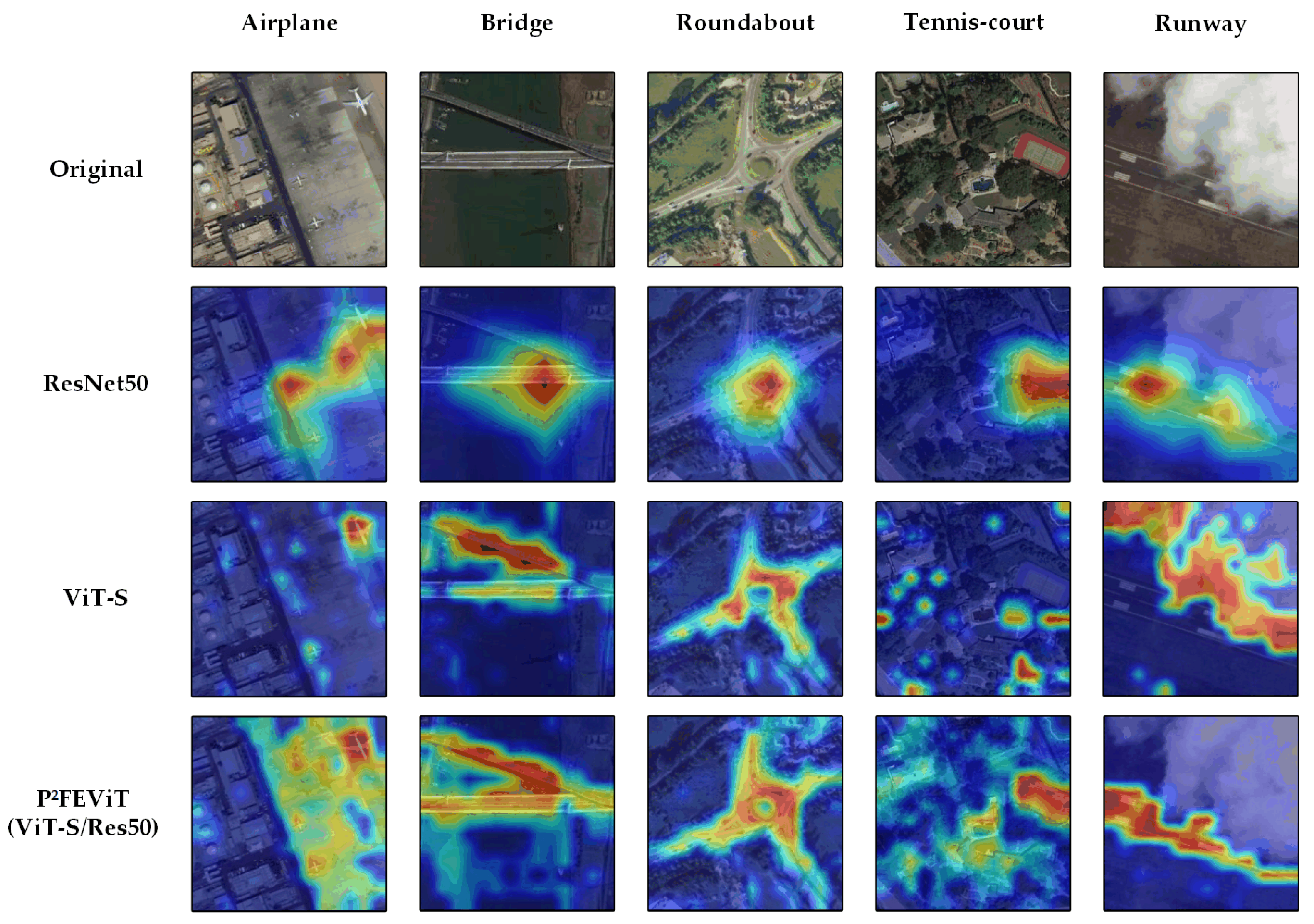
  66. Selvaraju, R.R.; Cogswell, M.; Das, A.; Vedantam, R.; Parikh, D.; Batra, D. Grad-cam: Visual explanations from deep networks via gradient-based localization. In Proceedings of the IEEE International Conference on Computer Vision, Venice, Italy, 22–29 October 2017; pp. 618–626. [Google Scholar]
  67. Al-Rfou, R.; Choe, D.; Constant, N.; Guo, M.; Jones, L. Character-level language modeling with deeper self-attention. In Proceedings of the AAAI Conference on Artificial Intelligence, Honolulu, HI, USA, 27 January–1 February 2019; Volume 33, pp. 3159–3166. [Google Scholar]
  68. Guo, Y.; Ji, J.; Lu, X.; Huo, H.; Fang, T.; Li, D. Global-local attention network for aerial scene classification. IEEE Access 2019, 7, 67200–67212. [Google Scholar] [CrossRef]
  69. He, N.; Fang, L.; Li, S.; Plaza, J.; Plaza, A. Skip-connected covariance network for remote sensing scene classification. IEEE Trans. Neural Netw. Learn. Syst. 2019, 31, 1461–1474. [Google Scholar] [CrossRef] [Green Version]
  70. Guo, D.; Xia, Y.; Luo, X. Scene classification of remote sensing images based on saliency dual attention residual network. IEEE Access 2020, 8, 6344–6357. [Google Scholar] [CrossRef]
  71. Tang, X.; Ma, Q.; Zhang, X.; Liu, F.; Ma, J.; Jiao, L. Attention consistent network for remote sensing scene classification. IEEE J. Sel. Top. Appl. Earth Obs. Remote Sens. 2021, 14, 2030–2045. [Google Scholar] [CrossRef]
  72. Li, Q.; Yan, D.; Wu, W. Remote sensing image scene classification based on global self-attention module. Remote Sens. 2021, 13, 4542. [Google Scholar] [CrossRef]
  73. Tan, M.; Le, Q. Efficientnet: Rethinking model scaling for convolutional neural networks. In Proceedings of the International Conference on Machine Learning, Long Beach, CA, USA, 9–15 June 2019; pp. 6105–6114. [Google Scholar]
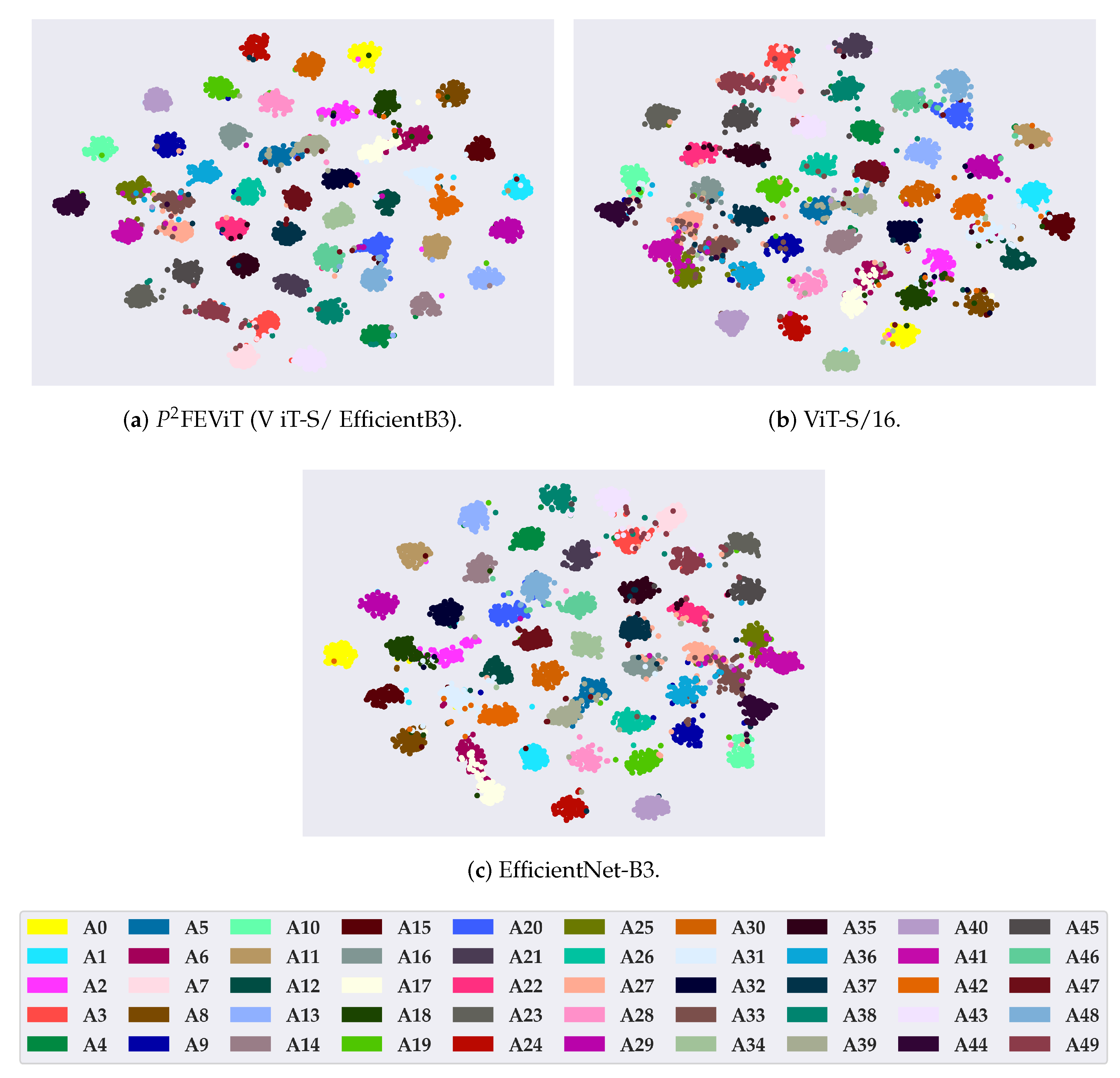
  74. Van der Maaten, L.; Hinton, G. Visualizing data using t-SNE. J. Mach. Learn. Res. 2008, 9, 2579–2605. [Google Scholar]
Figure 1. Instance samples in NWPU-RESISC45 dataset [24]. (a) presents different examples of the same category. (b) presents instance examples of different categories.
Remotesensing 15 01773 g001
Figure 2. Top1 accuracy of ViT-S/16 and ResNet50 under different initialization.
Remotesensing 15 01773 g002
Figure 3. Original images in NWPU-R45 [24] and their attention maps in CNN and ViT. (a)∼(d) refer to four different airport scenes in the dataset.
Remotesensing 15 01773 g003
Figure 4. The original Vision Transformer architecture.
Remotesensing 15 01773 g004
Figure 5. The network architecture of the proposed P 2 FEViT. (a) refers to the overall architecture of our method, and (b) refers to the detailed structure of the CBlock.
Remotesensing 15 01773 g005
Figure 6. Instance count distribution in original and balanced BIT-AFGR50.
Remotesensing 15 01773 g006
Figure 7. Examples of aircraft targets in BIT-AFGR50.
Remotesensing 15 01773 g007
Figure 8. Instance samples in NWPU-R45.
Remotesensing 15 01773 g008
Figure 9. Confusion matrix of our P 2 FEViT (ViT-B/EffcientB0) on NWPU-R45 (train:test = 2:8).
Remotesensing 15 01773 g009
Figure 10. Confusion matrix of our P 2 FEViT (ViT-B/ResNet50) on NWPU-R45 (train:test = 2:8).
Remotesensing 15 01773 g010
Figure 11. Samples of different categories with high inter-class similarities in NWPU-R45.
Remotesensing 15 01773 g011
Figure 12. Overall accuracy on BIT-AFGR50 under different initialization conditions. (a) fine-tuned with ImageNet pre-trained weights. (b) trained from scratch.
Remotesensing 15 01773 g012
Figure 13. Confusion matrix of our P 2 FEViT (ViT-S/EfficientB3) on BIT-AFGR50 (train:test = 2:8).
Remotesensing 15 01773 g013
Figure 14. Confusion matrix of our P 2 FEViT (ViT-S/ResNet50) on BIT-AFGR50 (train:test = 2:8).
Remotesensing 15 01773 g014
Figure 15. Attention maps of ViT-S/16, ResNet50 and our P 2 FEViT (VIT-S/ResNet50).
Remotesensing 15 01773 g015
Figure 16. Two-dimensional scatterplots of high-dimensional features on the BIT-AFGR50 dataset (training ratio = 20%). (a) P 2 FEViT (V iT-S/ EfficientB3). (b) ViT-S/16. (c) EfficientNet-B3.
Remotesensing 15 01773 g016
Table 1. Comparisons among publicly available optical RSIC datasets.
DatasetCategoriesImagesImage Width
NWPU-R45 [24]4531,500256
UC Merced Land-Use [36]212100256
Aerial Image Dataset [61]3010,000600
FGSCR-42 [63]42932050∼1500
BIT-AFGR50 15012,500128
1 BIT-AFGR50 refers to the balanced version.
Table 2. Overall accuracy (OA) of comparison SOTA methods under different training ratios on the NWPU-R45 dataset.
Method10% Training Ratio20% Training RatioYear, Publication
ResNet50 [16]92.40 ± 0.0794.22 ± 0.202016, CVPR
EfficientNet-B0 [73]91.79 ± 0.1994.71 ± 0.132019, ICML
EfficientNet-B1 [73]91.84 ± 0.1894.36 ± 0.142019, ICML
EfficientNet-B2 [73]92.17 ± 0.1294.65 ± 0.162019, ICML
EfficientNet-B3 [73]93.23 ± 0.1795.03 ± 0.172019, ICML
GLANet [68]91.03 ± 0.1893.45 ± 0.172019, IEEE Access
SCCov [69]89.30 ± 0.3591.10 ± 0.252019, IEEE TNNLS
ViT-S/16 [20]92.48 ± 0.1194.17 ± 0.052020, ICLR
ViT-B/16 [20]93.25 ± 0.0894.95 ± 0.072020, ICLR
SDAResNet50 [70]89.4092.282020, IEEE Access
ACNet [71]91.09 ± 0.1392.42 ± 0.162021, IEEE JSTARS
Li et al. [72]92.11 ± 0.0694.00 ± 0.132021, Remote Sensing
SCViT [34]92.72 ± 0.0494.66 ± 0.102021, IEEE TGRS
Cheng et al. [25]93.43 ± 0.2595.51 ± 0.212022, Remote Sensing
CTNet(ResNet34) [56]93.86 ± 0.2295.49 ± 0.122022, IEEE GRSL
CTNet(MobileNet_v2) [56]93.90 ± 0.1495.40 ± 0.152022, IEEE GRSL
P 2 FEViT (ViT-S 1 /ResNet50)93.43 ± 0.1294.79 ± 0.08ours
P 2 FEViT (ViT-S 1 /EfficientB0)93.52 ± 0.1195.41 ± 0.12
P 2 FEViT (ViT-S 1/EfficientB1)93.54 ± 0.0895.31 ± 0.13
P 2 FEViT (ViT-S 1 /EfficientB2)94.65 ± 0.1095.38 ± 0.12
P 2 FEViT (ViT-S 1 /EfficientB3)94.43 ± 0.0995.24 ± 0.18
P 2 FEViT(ViT-B 1 /EfficientB0)94.72 ± 0.0495.85 ± 0.15
P 2 FEViT(ViT-B 1/ResNet50)94.97 ± 0.1395.74 ± 0.19
1 All the ViT models are applied with patch size 16.
Table 3. Overall accuracy (OA) and training epoch of comparison methods with the different initial state on the BIT-AFGR50 dataset.
MethodInitial StateOATraining Epoch
PretrainedScratch
ResNet50 [16] 94.01 ± 0.17400
EfficientNet-B0 [73] 91.94 ± 0.07400
EfficientNet-B1 [73] 92.90 ± 0.12400
EfficientNet-B2 [73] 92.96 ± 0.09400
EfficientNet-B3 [73] 94.03 ± 0.06400
ViT-S/16 [20] 92.82 ± 0.11400
ViT-B/16 [20] 94.91 ± 0.13400
P 2 FEViT 1 92.94 ± 0.13150
P 2 FEViT 2 93.04 ± 0.1190
P 2 FEViT 3 95.02 ± 0.08200
P 2 FEViT 1 94.78 ± 0.15400
P 2 FEViT 2 95.46 ± 0.17400
P 2 FEViT 3 95.22 ± 0.13400
ResNet50 [16] 58.29 ± 0.17400
EfficientNet-B3 [73] 47.55 ± 0.17400
ViT-S/16 [20] 56.79 ± 0.11400
ViT-B/16 [20] 67.07 ± 0.13400
P 2 FEViT 2 57.53 ± 0.11220
P 2 FEViT 2 67.18 ± 0.15280
P 2 FEViT 2 74.92 ± 0.13400
P 2 FEViT 1 57.24 ± 0.05180
P 2 FEViT 1 67.57 ± 0.11250
P 2 FEViT 1 76.80 ± 0.17400
1 refers to the P2FEViT (ViT-S/ResNet50), and the ViT-S is applied with patch size 16. 2 refers to the P2FEViT (ViT-S/EfficientB3), and the ViT-S is applied with patch size 16. 3 refers to the P2FEViT (ViT-B/EfficientB3), and the ViT-B is applied with patch size 16.
Table 4. RSIC performance under different training ratios on BIT-AFGR50.
Method10% Training Ratio20% Training Ratio30% Training Ratio
EfficientNet-B0  [73]81.61 ± 0.1391.94 ± 0.0794.93 ± 0.03
EfficientNet-B1  [73]82.21 ± 0.1292.90 ± 0.1295.27 ± 0.10
EfficientNet-B2  [73]84.28 ± 0.1992.96 ± 0.0995.29 ± 0.05
EfficientNet-B3  [73]84.98 ± 0.0394.03 ± 0.0696.11 ± 0.05
ResNet50  [16]86.65 ± 0.1394.01 ± 0.1796.20 ± 0.09
ViT-S/16  [20]84.72 ± 0.1692.82 ± 0.1195.36 ± 0.08
ViT-B/16  [20]88.55 ± 0.1794.91 ± 0.1396.75 ± 0.08
P 2 FEViT (ViT-S 1/EfficientB3)88.50 ± 0.1195.46 ± 0.1797.22 ± 0.08
P 2 FEViT (ViT-S 1/ResNet50)89.30 ± 0.0794.78 ± 0.1597.12 ± 0.09
P 2 FEViT (ViT-B 1/EfficientB3)89.24 ± 0.1095.22 ± 0.1397.27 ± 0.15
1 All the ViT models are applied with patch size 16.
Disclaimer/Publisher’s Note: The statements, opinions and data contained in all publications are solely those of the individual author(s) and contributor(s) and not of MDPI and/or the editor(s). MDPI and/or the editor(s) disclaim responsibility for any injury to people or property resulting from any ideas, methods, instructions or products referred to in the content.

